Sub-percentage measure of distances to redshift of 0.1 by a new cosmic ruler
Abstract
Distance-redshift diagrams probe expansion history of the Universe. We show that the stellar mass-binding energy (massE) relation of galaxies proposed in our previous study offers a new distance ruler at cosmic scales. By using elliptical galaxies in the main galaxy sample of the Sloan Digital Sky Survey Data Release 7, we construct a distance-redshift diagram over the redshift range from 0.05 to 0.2 with the massE ruler. The best-fit dark energy density is 0.6750.079 for flat CDM, consistent with those by other probes. At the median redshift of 0.11, the median distance is estimated to have a fractional error of 0.34%, much lower than those by supernova (SN) Ia and baryonic acoustic oscillation (BAO) and even exceeding their future capability at this redshift. The above low- measurement is useful for probing dark energy that dominates at the late Universe. For a flat dark energy equation of state model (flat CDM), the massE alone constrains to an error that is only a factor of 2.2, 1.7 and 1.3 times larger than those by BAO, SN Ia, and cosmic microwave background (CMB), respectively.
keywords:
galaxies: general; galaxies: kinematics and dynamics; cosmology: observations; cosmology: cosmological parameters1 Introduction
A distance-redshift diagram is a powerful probe of the cosmic expansion history. The measurement by E. Hubble and G. Lemaître revealed the expansion of the Universe (Hubble, 1929; Lemaître, 1927), laying down the foundation of the big bang theory. In the past decades, two independent distance rulers at cosmic scales with appreciable redshifts, supernova Ia (SN Ia) and baryonic acoustic oscillation (BAO), demonstrated unambiguously the acceleration of the cosmic expansion, implying the existence of dark energy (Riess et al., 1998; Perlmutter et al., 1999; Eisenstein et al., 2005).
It is essential to have independent rulers to measure the distance vs. redshift diagram. Physically, different rulers probe the cosmic geometry from different aspects, thus examining a concordant cosmological model. Technically, each ruler has “nuisance” parameters that are unrelated to the cosmological parameters but can introduce systematic errors (e.g. Zuntz et al., 2015). Joint analysis by combining different rulers can significantly alleviate the degeneracy among cosmological parameters and improve their accuracy.
Uncertainties of current distance measurements using SN Ia and BAO are around a few percent and vary with redshift, mainly limited by the sample size and survey volume (Ross et al., 2015; Alam et al., 2017; Scolnic et al., 2018). In the forthcoming 5-10 years, large imaging and spectroscopic surveys will reach precision from a few sub-percent to one percent per redshift bin of 0.1 (Feng et al., 2014; DESI Collaboration et al., 2016). In this letter, we show that the relation between stellar masses and binding energies of galaxies as proposed in Shi et al. (2021) offers distance rulers at cosmic scales with significant statistical power. Through the study we will refer this relation as massE where “mass” stands for stellar masses and “E” for binding energies.
2 The massE cosmic ruler
Shi et al. (2021) demonstrated a tight relation between stellar mass and binding energy of galaxies, which covers nine orders of magnitude in stellar masses over a large range of galaxy types and redshift. The overall relationship is described by double power laws with the transition galaxy stellar mass of 107-108 M⊙. As illustrated in their Fig. 2 and 3, the dependence on redshift is absent up to 2.5, so does the dependence on galaxy properties such as galaxy sizes, surface densities and star formation rates. The physical origin of the massE relation may be related to the self-regulation of a galaxy between its binding energy and the accumulative feedback energy from its stellar populations. Although the massE relation holds for various types of galaxies, in this study we only use elliptical galaxies so that the velocity dispersion can be measured through single fibers.
For galaxies with stellar masses well above 108 M⊙, the massE relation can be written as a single power law:
| (1) |
where is the effective radius that encloses half of stellar light, is the total stellar masses of galaxies, is the velocity dispersion within for dispersion-dominated galaxies, and =0.40360.0016 (see § 3). represents the fourth root of the galaxy binding energies within .
In Equation 1, is independent of redshift, = and =, where is the apparent effective radius in arcsec, is the galaxy stellar mass placed at a distance of 1 Mpc, the angular diameter distance is related to the luminosity distance in =/(1+)2. can be obtained by first redshifting the observed spectral energy distribution (SED) to the rest-frame and then fit with stellar population synthesis models to obtain the mass-to-light ratio and the corresponding mass at a distance of 1 Mpc. is essentially a flux-like quantity and its measurement is independent of cosmological models.
As a result, the corresponding angular diameter distance calculator is:
| (2) | |||||
with =( in Mpc. When applying Equation 2 to estimate distances for cosmological purpose, the exact always degenerates with the local Hubble constant , similar to the case of the absolute magnitude of SN Ia. As a result, a nuisance parameter is included as the scaling factor for a sample to reproduce the local Hubble constant, and is related to the absolute calibration of three observables (, , ). The second nuisance parameter can be estimated from local samples as detailed in § 3.
Not that although the massE relation invokes the same three observables as the fundamental plane, they are different both physically and quantitatively. As shown in Shi et al. (2021), the massE is a correlation between galaxy stellar masses and binding energies while the fundamental plane is between galaxy stellar mass and dynamical masses. For galaxies above 108 , the massE relation only has two free parameters that are and in Equation 1, while the fundamental plane has three free parameters that are , and in Equation 5 of Shi et al. (2021). Furthermore, it has been known that the fundamental plane needs a fourth hidden systematic parameter to account for the dependence on galaxy properties or local environments (e.g. Bernardi et al., 2003; Magoulas et al., 2012; Howlett et al., 2022). As a result, the fundamental plane is mainly limited to z 0.05-0.1 for peculiar velocity studies (e.g. Howlett et al., 2022).
The following strategy is proposed to measure the distance vs. redshift diagram using the massE cosmic ruler. For a selected sample in a given redshift bin, its median redshift, if ignoring the peculiar velocity, corresponds exactly to its median luminosity distance, because the luminosity distance increases monotonically with redshift, independent of cosmological models. As a result, we measure the median of the redshift distribution and the median of the luminosity distance distribution in individual redshift bins to obtain the distance vs. redshift diagram. With this strategy, the sample incompleteness does not matter, i.e., objects rejected by the selection function does not affect at all the correspondence between the median distance and median redshift. But the Malmquist bias does matter in a way that, e.g., a sample with a magnitude cut is intrinsically fainter so that their stellar mass is over-estimated.


3 The massE relationship of the local sample
Before applying the massE to the SDSS sample, we first need to estimate the intrinsic massE relationship, especially in Equation 1. We thus perform the fitting to the sample compiled and homogenized in Shi et al. (2021), while excluding luminous infrared galaxies and ultra diffuse galaxies because of their large observational errors as well as high- sources in order to remove the dependence of the relationship on the cosmological model. This local sample contains 589 objects as shown in Fig. 1. Measurements of galaxy sizes, velocity dispersions and stellar masses of the sample in general have high signal to noise. We thus add additional 0.1 dex, 10% and 1% systematic errors quadratically to , and , respectively. The systematic error for is mainly caused by uncertainties in population synthetic modeling, which can be illustrated by comparing the MPA-JHU and CIGALE stellar masses of SDSS galaxies in § 6.1. The uncertainty for is from background subtraction, morphology irregularity, galaxy center determination etc. We estimated this by selecting a subsample of SDSS galaxies with high signal-to-noise ratio 100 and comparing measurements from different data releases. The systematic error for is mainly caused by absolute wavelength calibration and 1% is a reasonable estimate for modern CCD-based spectra (Law et al., 2021). If increasing the errors by a small amount, e.g., to 0.15 dex for , to 15% for and to 2% for , respectively, the difference in the derived slope is within one .
We performed PyMC3 (Salvatier et al., 2016) by considering errors on both and to obtain the intrinsic relationship. The best fit gives =0.40360.0016 and the corresponding co-varies with through:
| (3) |
The derived slope is similar to that in Shi et al. (2021) but with a smaller error, because in Shi et al. (2021) the fitting was done without weighting by observational errors, which thus gives the result including the observational error instead of the intrinsic relationship. Distances of this local sample are mostly below 40 Mpc, with the remaining 17% of the sample distributes between 40 and 300 Mpc. They are mainly based on cosmological-independent measurements for those below 20 Mpc, but are homogenized to a flat CDM with =73 km/s/Mpc, and =0.73 for those above 20 Mpc. However, the best-fit changes only by a small fraction of its 1- error if changing to =1.0 or =0.4, respectively. This is because the associated change in and is much smaller than their observational errors, plus the fact that both X and Y-axes vary simultaneously to partially cancel out the effect.
We also carry out additional fitting to the massE relationship by including 105 high- objects compiled in Shi et al. (2021). The derived =0.40450.0016 is essentially the same as the one with only the local sample. This suggests that should not evolve strongly with the redshift.
4 Elliptical galaxies in the main galaxy sample of Sloan Digital Sky Survey (SDSS)
Although all types of galaxies can be used for the massE ruler, elliptical galaxies are the most suitable ones given their low extinction, regular morphologies, low current star formation rates and dispersion dominated kinematics, which will facilitate measurements of three observables (, , ). Unlike spiral galaxies whose velocity requires spatially-resolved kinematic maps, ellipticals’ can rely on single-fiber measurements (Cappellari et al., 2006; Shi et al., 2021). We build our elliptical galaxy sample from the value-added MPA-JHU catalog (Kauffmann et al., 2003; Brinchmann et al., 2004) of the SDSS data release 7 111https://wwwmpa.mpa-garching.mpg.de/SDSS/DR7/. A sample of about 28,0000 elliptical galaxies were selected from the SDSS main galaxy sample with the following criteria: (1) no redshift warning as indicated by Z_WARNING=0; (2) the main galaxy sample as defined by PRIMTARGET 64 but 128 and Petrosion magnitude in 17.77; (3) elliptical galaxies as defined by FRACDEV 0.8. Only the second criterion will introduce the Malmquist bias while others are not related to the three observables (, , ).
To apply Equation 2, we adopt the Petrosian radius in the band (PETROR50_R) to represent . The total stellar mass adopts MSTAR_TOT that is derived from fitting to Petrosian magnitudes in four SDSS optical bands. The advantage of the Petrosian radius and magnitude is that there is no bias in redshift due to the surface dimming (Blanton et al., 2001), which is the key for the distance vs. redshift measurement. is converted to simply through the adopted cosmology for the MPA-JHU catalog.
We carry out our own measurements of the velocity dispersion, because those in the MPA-JHU catalog were derived by using the median instrumental resolution, which will introduce redshift-dependent bias as the true instrumental resolution is a function of the wavelength. The spectrum and associated wavelength-dependent instrumental resolution of each object were available in the SDSS archive222http://data.sdss.org/sas/dr12/sdss/spectro/redux/26/spectra/. The fitting was done using the pPXF code (Cappellari, 2017) by adopting the HR-PYPOPSTAR theoretical stellar populations with 50,000 resolving power at 5000Å (Millán-Irigoyen et al., 2021). During the fitting, we further exclude 5800-6100Å range where blue and red channels of the spectrograph with different instrumental resolutions overlap. The derived velocity dispersion within a 3′′ fiber was then corrected to that at PETROR50_R by the following equation (Cappellari et al., 2006):
| (4) |
Here the error on the power-law index is implemented through numpy.random.normal.


5 The distance vs. redshift diagram of the SDSS elliptical sample.
| ID | ln() | |
|---|---|---|
| ln(Mpc) | ||
| 1 | 0.0549 | 5.5840 |
| 2 | 0.0652 | 5.7371 |
| 3 | 0.0752 | 5.8830 |
| 4 | 0.0847 | 5.9884 |
| 5 | 0.0950 | 6.0851 |
| 6 | 0.1051 | 6.1746 |
| 7 | 0.1150 | 6.2391 |
| 8 | 0.1251 | 6.2892 |
| 9 | 0.1348 | 6.3628 |
| 10 | 0.1449 | 6.4589 |
| 11 | 0.1546 | 6.5070 |
| 12 | 0.1649 | 6.5449 |
| 13 | 0.1749 | 6.6054 |
| 14 | 0.1846 | 6.6676 |
| 15 | 0.1948 | 6.6847 |
| 82.38 | 0.49 | 0.83 | 0.96 | 1.24 | 1.45 | 1.64 | 1.79 | 2.01 | 2.34 | 2.49 | 2.69 | 3.01 | 3.16 | 3.27 |
| 0.49 | 51.29 | 1.28 | 1.47 | 1.88 | 2.23 | 2.48 | 2.71 | 3.01 | 3.52 | 3.72 | 3.96 | 4.47 | 4.69 | 4.87 |
| 0.83 | 1.28 | 36.32 | 2.48 | 3.20 | 3.76 | 4.22 | 4.62 | 5.18 | 6.05 | 6.42 | 6.92 | 7.77 | 8.12 | 8.44 |
| 0.96 | 1.47 | 2.48 | 36.24 | 3.75 | 4.40 | 4.93 | 5.41 | 6.05 | 7.08 | 7.52 | 8.13 | 9.10 | 9.49 | 9.88 |
| 1.24 | 1.88 | 3.20 | 3.75 | 45.49 | 5.69 | 6.38 | 7.00 | 7.84 | 9.16 | 9.73 | 10.53 | 11.80 | 12.30 | 12.80 |
| 1.45 | 2.23 | 3.76 | 4.40 | 5.69 | 45.02 | 7.49 | 8.21 | 9.20 | 10.76 | 11.41 | 12.34 | 13.85 | 14.44 | 15.02 |
| 1.64 | 2.48 | 4.22 | 4.93 | 6.38 | 7.49 | 37.99 | 9.21 | 10.32 | 12.06 | 12.80 | 13.85 | 15.53 | 16.20 | 16.85 |
| 1.79 | 2.71 | 4.62 | 5.41 | 7.00 | 8.21 | 9.21 | 45.24 | 11.34 | 13.25 | 14.07 | 15.22 | 17.07 | 17.80 | 18.51 |
| 2.01 | 3.01 | 5.18 | 6.05 | 7.84 | 9.20 | 10.32 | 11.34 | 45.28 | 14.86 | 15.79 | 17.10 | 19.17 | 19.99 | 20.79 |
| 2.34 | 3.52 | 6.05 | 7.08 | 9.16 | 10.76 | 12.06 | 13.25 | 14.86 | 53.22 | 18.44 | 19.98 | 22.40 | 23.36 | 24.29 |
| 2.49 | 3.72 | 6.42 | 7.52 | 9.73 | 11.41 | 12.80 | 14.07 | 15.79 | 18.44 | 55.99 | 21.24 | 23.79 | 24.81 | 25.81 |
| 2.69 | 3.96 | 6.92 | 8.13 | 10.53 | 12.34 | 13.85 | 15.22 | 17.10 | 19.98 | 21.24 | 67.13 | 25.81 | 26.89 | 27.98 |
| 3.01 | 4.47 | 7.77 | 9.10 | 11.80 | 13.85 | 15.53 | 17.07 | 19.17 | 22.40 | 23.79 | 25.81 | 70.35 | 30.15 | 31.36 |
| 3.16 | 4.69 | 8.12 | 9.49 | 12.30 | 14.44 | 16.20 | 17.80 | 19.99 | 23.36 | 24.81 | 26.89 | 30.15 | 79.61 | 32.69 |
| 3.27 | 4.87 | 8.44 | 9.88 | 12.80 | 15.02 | 16.85 | 18.51 | 20.79 | 24.29 | 25.81 | 27.98 | 31.36 | 32.69 | 88.80 |
All numbers are in 10-6 ln(Mpc)2. Each number gives the covariance between -th and -th redshift bins as listed in Table 1.
The redshift distribution of the SDSS elliptical sample peaks around 0.11. We limit the redshift range to [0.05, 0.2] and construct the distance vs. redshift diagram with a redshift bin size of 0.01. The number of galaxies in individual redshift bins result in negligible fractional errors of their median redshift, which is 0.06% for a random peculiar velocity of 1000 km/s. The upper range at =0.2 is also necessary to avoid the Malmquist bias caused by the magnitude cut of 17.77. Although the massE ruler is not subject to the sample completeness, objects that are selected into the sample can systematically bias the stellar mass if their luminosity is overestimated due to the Malmquist bias. To estimate it roughly, we use the -band luminosity function (Blanton et al., 2003) to construct a mock -band photometric sample down to the SDSS 5- depth (=22.7) at different redshifts, and add the photometric error based on the median and standard deviation of apparent magnitude errors as a function of magnitude from the SDSS sample. By assuming a constant mass-to-light ratio in the -band, it is found that the median distance is under-estimated by 1% at (,)=(0.2, 0.01) while by as much as 7% at (,)=(0.25, 0.01) for the sub-sample with 17.77. As a result, we limit the range to be below 0.2 so that the Malmquist bias is a small fraction of the typical 1- uncertainty in individual redshift bins that are around 1.3% including both observational errors and systematic errors in (see § 6.2).
As stated above, the massE ruler has two nuisance parameters: calibrates the absolute distance, which degenerates with the local Hubble constant, and determines the relative distances among galaxies with different masses. The latter is transformed to the curvature of the distance-redshift diagram, because for a flux limited sample galaxies at higher redshifts have higher masses. The massE ruler would be a viable new probe of cosmic expansion history, only if for a fixed the massE ruler gives a smooth function of the distance vs. redshift with small fluctuations, otherwise systematic errors unrelated to , e.g., some hidden parameters, may be too large for the massE ruler to be feasible. The latter is in fact the case for other galaxy scaling laws. As a sanity check, we let uniformly distribute over a very large range from 0 to 1, and carry out the fitting with flat CDM through cosmosis (Zuntz et al., 2015) and emcee sampler (Foreman-Mackey et al., 2013). As listed in Table 3, converges to be a reasonable value, i.e., 0.540.28, along with =0.410.09. This indicates that once is estimated from the local relationship, the performance of the massE ruler can further improve.
Figure 2 (a) shows the derived distance-redshift diagram in terms of ln() as a function of redshift, which is also listed in Table 1. As shown in Figure 3 (a) and listed in Table 2, the covariance matrix of ln() includes two parts. The first one is caused by the observational errors of , and . In the case of no observational errors, the derived distribution should be the redshift distribution convolved with peculiar velocity. As an example shown in Figure 3 (b) for =[0.17, 0.18], the derived ln() distribution (blue filled) scatters much more broadly than that implied by the redshift distribution (orange filled). The distribution can be approximated with a central Gaussian core plus a broad wing. The standard deviation of the central core is 0.29, which is consistent with but slightly larger than the square root of the quadratic sum of quoted median errors of three observables in the catalog (red open symbols) through Equation 2, which gives 0.21. This indicates that the quoted errors of observables are slightly under-estimated. The broad wing is due to outliers of measurements. As a result, we adopt the standard deviation of the whole distribution divided by the square root of the number of objects as the error. It is about two times larger than the one derived by the bootstrap method. Since each redshift bin is independent, all non-diagonal elements of the covariance matrix are set to zero for this first part. The second part is due to the variation in . We adopt its measurement and associated error from the local sample to calculate the corresponding covariance matrix of ln(). Note that all uncertainties, e.g., the systematic uncertainties in the stellar initial mass function, which shifts all distances by the same amount, are taken into account by .
| priors† | for massE | rulers | |||
| flat CDM | |||||
| U(0, 1) | MPA-JHU | massE | 0.410.09 | 0.540.28 | – |
| fixed to N (0.40360.0016) | MPA-JHU | massE | – | 0.6750.079 | – |
| fixed to N (0.40360.0016) | CIGALE | massE | – | 0.6780.078 | – |
| flat CDM | |||||
| SN Ia | – | 0.68 | -1.06 | ||
| BAO | – | 0.72 | -0.73 | ||
| CMB | – | 0.80 | -1.49 | ||
| massE | – | 0.67 | -0.97 | ||
†U stands for a uniform distribution and N is for a normal distribution. All other priors are included in Table 4.
6 Constraints on cosmological parameters
6.1 Constraints on the flat CDM
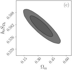
We carry out the fitting to the distance vs. redshift diagram in Figure 2 as obtained by the massE ruler with a flat CDM. The fitting was done through cosmosis (Zuntz et al., 2015) with the emcee sampler (Foreman-Mackey et al., 2013), whose priors are listed in Table 4 where both and are set to be free. As shown in Figure 2 (c), the convergent results have =0.6750.079, which is 1- consistent with constraints by BAO (Ross et al., 2015; Alam et al., 2017), SN Ia (Scolnic et al., 2018) and CMB (Planck Collaboration et al., 2020). The massE ruler thus proves the acceleration of the universe at 8.5- with elliptical galaxies in the SDSS main galaxy sample under flat CDM.
Among three observables, relies on the stellar population synthetic model, while the other two are straightforward measurements with weak model dependence. We thus carry out additional sets of stellar mass measurements and compared to the result of the MPA-JHU catalog. It is found that with multi-band broad SED, the systematic effect of measurements on the derived cosmological parameters is small as long as the parameter space of the population synthetic model is reasonably sampled. We use CIGALE (Boquien et al., 2019) to construct a two exponential decaying star formation history with the second one for the late-epoch burst. The fraction of models that experiences late bursts is 20%, smaller than 50% in MPA-JHU (Kauffmann et al., 2003). The metallicity is uniformly distributed among four discrete values that are 0.2, 0.4, 1.0 and 2.5 solar, while in MPA-JHU the metallicity is interpolated to a higher resolution. The interstellar medium extinction is uniform between 0.0 and 1.5, while the MPA-JHU catalog extends to higher values. Although the standard deviation of the difference between MPA-JHU’ and CICALE’ stellar masses reaches 20%, the systematic offset is much smaller. As listed in Table 3, the best-fit is 0.6780.078 for the flat CDM, which is essentially the same as the one (0.6750.079) with the MPA-JHU mass.
6.2 The statistical power in distance measure
To illustrate the statistical advantage in distance measure with the massE ruler, Figure 4 compares the fractional error of the massE-based distance to those by SN Ia and BAO. We sum the covariance matrix to obtain this error. In our redshift range of [0.05, 0.2] with a median redshift =0.11, the corresponding angular diameter distance is ln([Mpc])=6.19870.0034. This fractional distance error of 0.34% is a quadratic sum of 0.17% by errors of three observables and 0.3% by uncertainties. A double check of this estimate can be obtained by looking at the residual of the best fit as shown in Figure 2 (b). For each bin, the deviation from the true distance is caused by the statistical error of three observables plus one realization of the intrinsic massE relationship that is independent from other bins. As a result, the fluctuation in the residual should converge to the result by the covariance matrix if the number of redshift bins is large enough. An error of 0.35% is derived from the standard deviation of the residual for the median distance of the above redshift range, which is close to the one from the covariance matrix. We further check whether the Malmquist bias can affect this error estimate by calculating the bias for each redshift bin and treating it as additional independent error. It is found that the final fractional distance error increases negligibly from 0.35% to 0.36%.
As shown in the figure, the measurement with massE gives about one order of magnitude smaller fractional errors than existing measurements at similar redshift with SN Ia and BAO (Ross et al., 2015; Alam et al., 2017; Scolnic et al., 2018). As compared to next-generation surveys as offered by BAO from DESI and SN Ia from Rubin/Roman (Feng et al., 2014; DESI Collaboration et al., 2016), the massE ruler still offers 2-4 times smaller fractional error at 0.1. This demonstrates the statistical power of the massE ruler as a new probe of cosmic geometry.
The statistical power of the massE ruler can be understood in the following way. Although each SN Ia offers a fractional distance error of 5% as compared to 25% of the massE, the number of elliptical galaxies is far more numerous than the SN Ia. On the other hand, BAO is essentially volume-limited at low-.
6.3 Constraints on the dark energy equation of state CDM (CDM)
The low- distance measurements at high accuracy by massE is particularly useful to probe the deviation from the constant of the dark energy density that dominates at the low- universe. As shown in Figure 5, we illustrate this by carrying out constraints on the CDM model with the massE data and compare to those with the Pantheon SN Ia data (Scolnic et al., 2018), the MGS/BOSS/eBOSS BAO data (Ross et al., 2015; Alam et al., 2017, 2021) and the Planck 2018 CMB TT,TE,EE+lowE data (Planck Collaboration et al., 2020), respectively. All fittings have been done with cosmosis (Zuntz et al., 2015) and emcee sampler (Foreman-Mackey et al., 2013). As listed in Table 3, the massE alone constrains to an error that is only a factor of 2.2, 1.7 and 1.3 larger than the current one by BAO only, SN Ia only and CMB only, respectively.
7 Conclusion
In this study we have shown that the massE relationship of galaxies could be a new cosmic ruler to probe the distance-redshift diagram with advantage of its statistical power. It has two nuisance parameters with three observables for ellipticals that are galaxy sizes, velocity dispersions and stellar masses. With the SDSS MGS sample, the distance at =0.11 with the massE ruler is constrained to a fractional error of 0.34%, with the best-fit dark energy density of 0.6750.079 for flat CDM. In principle the massE can be applied to higher by combining large-area space-based imaging survey and ground-based deep spectroscopic survey.
The cosmosis modules including the input parameter files and data files for the massE can be obtained through the link available on arXiv of this manuscript.
Acknowledgements
We thank the referee for constructive comments that help improve the paper. We thank Pengjie Zhang for helpful comments. Y.S. acknowledges the support from the National Key Research and Development Program of China (No. 2018YFA0404502), the National Natural Science Foundation of China (NSFC grants 11825302, 12141301, 12121003, 11733002), the science research grants from the China Manned Space Project with NO. CMS-CSST-2021-B02, and the Tencent Foundation through the XPLORER PRIZE. S.M. is partly supported by the National Key Research and Development Program of China (No. 2018YFA0404501), by the National Natural Science Foundation of China (11821303, 11761131004 and 11761141012) and by Tsinghua University Initiative Scientific Research Program ID 2019Z07L02017. Z.Y.Z acknowledges the support of the National Natural Science Foundation of China (NSFC) under grants No. 12041305, 12173016, the Program for Innovative Talents, Entrepreneur in Jiangsu, and the science research grants from the China Manned Space Project with NO. CMS-CSST-2021-A08, CMS-CSST-2021-A07.
Funding for the SDSS and SDSS-II has been provided by the Alfred P. Sloan Foundation, the Participating Institutions, the National Science Foundation, the U.S. Department of Energy, the National Aeronautics and Space Administration, the Japanese Monbukagakusho, the Max Planck Society, and the Higher Education Funding Council for England. The SDSS Web Site is http://www.sdss.org/. The SDSS is managed by the Astrophysical Research Consortium for the Participating Institutions. The Participating Institutions are the American Museum of Natural History, Astrophysical Institute Potsdam, University of Basel, University of Cambridge, Case Western Reserve University, University of Chicago, Drexel University, Fermilab, the Institute for Advanced Study, the Japan Participation Group, Johns Hopkins University, the Joint Institute for Nuclear Astrophysics, the Kavli Institute for Particle Astrophysics and Cosmology, the Korean Scientist Group, the Chinese Academy of Sciences (LAMOST), Los Alamos National Laboratory, the Max-Planck-Institute for Astronomy (MPIA), the Max-Planck-Institute for Astrophysics (MPA), New Mexico State University, Ohio State University, University of Pittsburgh, University of Portsmouth, Princeton University, the United States Naval Observatory, and the University of Washington.
Data Availability
All the data used here are available upon reasonable request.
References
- Alam et al. (2017) Alam S., et al., 2017, MNRAS, 470, 2617
- Alam et al. (2021) Alam S., et al., 2021, Phys. Rev. D, 103, 083533
- Bernardi et al. (2003) Bernardi M., et al., 2003, AJ, 125, 1866
- Blanton et al. (2001) Blanton M. R., et al., 2001, AJ, 121, 2358
- Blanton et al. (2003) Blanton M. R., et al., 2003, ApJ, 592, 819
- Boquien et al. (2019) Boquien M., Burgarella D., Roehlly Y., Buat V., Ciesla L., Corre D., Inoue A. K., Salas H., 2019, A&A, 622, A103
- Brinchmann et al. (2004) Brinchmann J., Charlot S., White S. D. M., Tremonti C., Kauffmann G., Heckman T., Brinkmann J., 2004, MNRAS, 351, 1151
- Cappellari (2017) Cappellari M., 2017, MNRAS, 466, 798
- Cappellari et al. (2006) Cappellari M., et al., 2006, MNRAS, 366, 1126
- DESI Collaboration et al. (2016) DESI Collaboration et al., 2016, arXiv e-prints, p. arXiv:1611.00036
- Eisenstein et al. (2005) Eisenstein D. J., et al., 2005, ApJ, 633, 560
- Feng et al. (2014) Feng J. L., et al., 2014, arXiv e-prints, p. arXiv:1401.6085
- Foreman-Mackey et al. (2013) Foreman-Mackey D., Hogg D. W., Lang D., Goodman J., 2013, PASP, 125, 306
- Hinton (2016) Hinton S. R., 2016, The Journal of Open Source Software, 1, 00045
- Howlett et al. (2022) Howlett C., Said K., Lucey J. R., Colless M., Qin F., Lai Y., Tully R. B., Davis T. M., 2022, arXiv e-prints, p. arXiv:2201.03112
- Hubble (1929) Hubble E., 1929, Proceedings of the National Academy of Science, 15, 168
- Kauffmann et al. (2003) Kauffmann G., et al., 2003, MNRAS, 341, 33
- Law et al. (2021) Law D. R., et al., 2021, AJ, 161, 52
- Lemaître (1927) Lemaître G., 1927, Annales de la Société Scientifique de Bruxelles, 47, 49
- Magoulas et al. (2012) Magoulas C., et al., 2012, MNRAS, 427, 245
- Millán-Irigoyen et al. (2021) Millán-Irigoyen I., Mollá M., Cerviño M., Ascasibar Y., García-Vargas M. L., Coelho P. R. T., 2021, MNRAS, 506, 4781
- Perlmutter et al. (1999) Perlmutter S., et al., 1999, ApJ, 517, 565
- Planck Collaboration et al. (2020) Planck Collaboration et al., 2020, A&A, 641, A6
- Riess et al. (1998) Riess A. G., et al., 1998, AJ, 116, 1009
- Ross et al. (2015) Ross A. J., Samushia L., Howlett C., Percival W. J., Burden A., Manera M., 2015, MNRAS, 449, 835
- Salvatier et al. (2016) Salvatier J., Wieckiâ T. V., Fonnesbeck C., 2016, PyMC3: Python probabilistic programming framework (ascl:1610.016)
- Scolnic et al. (2018) Scolnic D. M., et al., 2018, ApJ, 859, 101
- Shi et al. (2021) Shi Y., Yu X., Mao S., Gu Q., Xia X., Chen Y., 2021, MNRAS, 507, 2423
- Zuntz et al. (2015) Zuntz J., et al., 2015, Astronomy and Computing, 12, 45
Appendix A Priors of cosmological parameters
The priors of cosmological parameters are detailed in Table 4. All fittings have been done with cosmosis (Zuntz et al., 2015) and emcee sampler (Foreman-Mackey et al., 2013). Each fitting has 4106 samples, with the Gelman-Rubin (G-R) convergence value of 0.01, except for CMB that has 15106 samples in order to have G-R value below 0.01.
| parameters | priors | models |
|---|---|---|
| massE only | ||
| U(0.0, 1.0) | flat CDM, flat CMD | |
| U(0.2, 1.0) | flat CDM, flat CMD | |
| U(0.3, 2.0) | flat CDM, flat CMD | |
| U(-3.0, 0.0) | flat CMD | |
| SN Ia only | ||
| U(0.0, 1.0) | flat CMD | |
| U(0.2, 1.0) | flat CMD | |
| U(-23, -15) | flat CMD | |
| U(-3.0, 0.0) | flat CMD | |
| BAO only | ||
| U(0.0, 1.0) | flat CMD | |
| U(0.2, 1.0) | flat CMD | |
| U(0.001, 0.3) | flat CMD | |
| U(-3.0, 0.0) | flat CMD | |
| CMB only | ||
| U(0.0, 0.9) | flat CMD | |
| U(0.0, 0.3) | flat CMD | |
| U(0.2, 1.0) | flat CMD | |
| U(-3.0, 0.0) | flat CMD | |
| U(0.8, 1.2) | flat CMD | |
| U(1.48, 5.45) | flat CMD | |
| 0.05 | flat CMD | |
| U(0.01, 0.8) | flat CMD | |
U stands for a uniform distribution.