Study of the process at center-of-mass energies between 4.0 and 4.6 GeV
Abstract
Using of collision data collected at twenty-four center-of-mass energies from to GeV with the BESIII detector, the helicity amplitudes of the process are analyzed for the first time. Born cross section measurements of two-body intermediate resonance states with statistical significance greater than 5 are presented, such as , , , , , and . In addition, evidence of a resonance state in production is found. The mass of this state obtained by line shape fitting is about GeV/, which is consistent with the production of or .
Keywords:
Charmonium (-like), Born cross section measurement, helicity amplitude analysis1 INTRODUCTION
In recent years the study of charmonium-like() states has become a hot topic for both experimental and theoretical physics due to their unexpected resonance parameters and exotic decay patterns pdg . Since , a series of charmonium-like states inconsistent with the quark model, such as the ref5 , ref6 and ref7 ; ref8 , have been observed. In particular, the vector charmonium-like state was observed by the BaBar experiment in ref6 and was confirmed by the CLEO and Belle experiments ref9 ; ref10 . In , the BESIII experiment performed a dedicated scan of and observed two structures in this energy region. The one with the mass MeV/ ref11 was regarded as the previously observed , and renamed as . The was then confirmed in the Born cross section line shapes of ref12 , ref13 , ref14 , and ref15 measured by the BESIII experiment. The other structure was identified with the , which was previously observed in by the BaBar experiment in ref16 . Theoretically, many assignments, such as a tetraquark state ref3 ; ref4 ; a1 ; a2 ; a3 ; a4 ; a5 ; a6 , a hybrid state ref2 ; b1 ; b2 ; b3 ; b4 , a hadro-charmonium state c1 ; c2 ; c3 ; c4 , a molecular state d1 ; d2 ; d3 ; d4 , a kinematic effect e1 ; e2 ; e3 ; e4 , a baryonium state f1 , etc., were proposed to explain the state.
The traditional charmonium states, such as and , were observed in dasp ; bes2 ; rvue and psi4160 . However, their decays into light hadron final states have never been observed. Many searches have been performed for these charmonium(-like) states produced in collisions and decaying to light hadron final states, including kkpipi0 , kkpi , 4p , and 4040 . Only evidence for has been reported.
In this paper, we measure the Born cross sections of at 24 center-of-mass (c.m.) energies between 4.0 and 4.6 GeV, to search for the charmonium(-like) states decaying into light hadron final sates. Furthermore, we study intermediate states in the process via partial wave analysis (PWA).
2 BESIII DETECTOR AND MONTE CARLO SIMULATION
The BESIII detector is a magnetic spectrometer BESIII located at the Beijing Electron Positron Collider (BEPCII) BEPCII . The cylindrical core of the BESIII detector consists of a helium-based multilayer drift chamber (MDC), a plastic scintillator time-of-flight system (TOF), and a CsI(Tl) electromagnetic calorimeter (EMC), which are all enclosed in a superconducting solenoidal magnet providing a T magnetic fielddetvis . The solenoid is supported by an octagonal flux-return yoke with resistive plate counter muon identifier modules interleaved with steel. The acceptance of charged particles and photons is over solid angle. The charged-particle momentum resolution at is , and the specific ionization energy loss () resolution is for the electrons from Bhabha scattering. The EMC measures photon energies with a resolution of () at GeV in the barrel (end cap) region. The time resolution of the TOF barrel part is ps, while that of the end cap part is ps. The end cap TOF system was upgraded in with multi-gap resistive plate chamber technology, providing a time resolution of ps tof ; about 84% of the data used here benefits from this improvement.
This analysis uses data sets taken at twenty-four c.m. energies ranging from 4.0 to 4.6 GeV. For each data set, the c.m. energy is calibrated by the di-muon process mumu , where stands for possible initial state radiative (ISR) or final state radiative (FSR) photons. The integrated luminosity () is determined using large-angle Bhabha events rlum , and the total integrated luminosity of all data sets is fb-1.
The BESIII detector is modeled with a Monte Carlo (MC) simulation using the software framework BOOST boost , based on GEANT4 geant4 , which includes the geometric and material description of the BESIII detector geo1 ; geo2 , the detector response, and digitization models, as well as the detector running conditions and performances. Simulated MC samples generated by a phase space (PHSP) model with kkmc kkmc are used for efficiency corrections in the PWA, and the TOY MC samples with detector simulation generated by ConExc besevtgen are used to determine detection efficiencies used for the Born cross-section determinations. The TOY MC events are generated based on helicity amplitude model with parameters fixed to the PWA results. The inclusive MC sample generated at GeV with kkmc kkmc is used to study the potential backgrounds.
3 EVENT SELECTION AND BACKGROUND ANALYSIS
For , , , the final state is characterized by four charged pion tracks and two photons. For each charged track, the distance of closest approach to the interaction point is required to be within cm in the beam direction and within cm in the plane perpendicular to the beam direction. The track polar angle () must be within the fiducial volume of the MDC, , . Particle identification (PID) for charged tracks combines the d/d and TOF information to form likelihoods for each particle hypothesis. Momentum-dependent PID is used to improve detection efficiency. Charged tracks with momentum less than 0.9 GeV/, are identified as pion candidates if their likelihoods satisfy and . Those with momentum greater than GeV/ are assigned as pion candidates with no PID requirement.
Isolated EMC showers are considered as photon candidates. The deposited energy of each shower must be above MeV in the barrel region () and MeV in the end cap region (). Showers are required to occur within ns of the event start time to suppress noise. Photon pairs with an invariant mass in the interval GeV/ are taken as candidates.
To reduce potential peaking backgrounds from with converting to , the of the pion candidate from non- decay is required to be less than , where and are momentum and EMC energy deposit associated with the track, respectively. To suppress the backgrounds from and xc0 , the invariant mass of all four combinations are required to be outside the range of (, ) and (, ) GeV/, respectively. To further suppress the background and improve the mass resolution, we perform a five-constraint (C) kinematic fit to the known initial four-momentum and mass pdg . The under the hypothesis of with is required to be less than . If more than one combination satisfies the above selection requirements, only the one with the smallest is kept. To suppress background contribution from the final states with an additional photon, the under the hypothesis is required to be less than that under the hypothesis: .
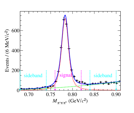
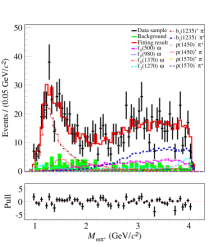
In each event, there are four combinations; the one with the invariant mass closest to the known mass pdg is chosen as the candidate. This may distort the combinatoric background shape. A study of an MC sample leads to a smooth distribution of the invariant mass of combinatoric that can be described by a polynomial function. A study based on the signal MC sample shows that the ratio of the yield of combinatoric background to the signal yield is % and results in a negligible difference of % on the fitted signal yield. Figure 1 shows the distribution of the accepted events from the data sample taken at GeV. To extract the number of signal events, an unbinned extended maximum-likelihood fit is performed on the distribution. The signal shape is a MC-derived shape convolved with an additional Gaussian smearing function, and the background shape is a second-order Chebychev polynomial function. The signal yields are listed in Table 3. Based on the resolution from fitting, the signal region is defined as GeV/, while the sideband regions are defined as the regions GeV/ and GeV/.
4 AMPLITUDE ANALYSIS
4.1 Kinematic variable and helicity angles
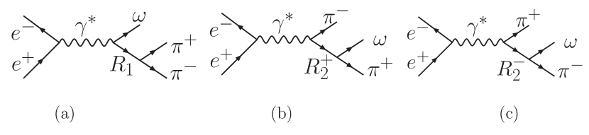
The final sate is produced from the annihilation into a virtual photon, followed by hadronization into the final sate, where ( , , ) denote particle momenta after the kinematic fit. The final state may be produced non-resonantly, or via an intermediate resonance and subsequent decay; the possible resonance diagrams are shown in Fig. 2.
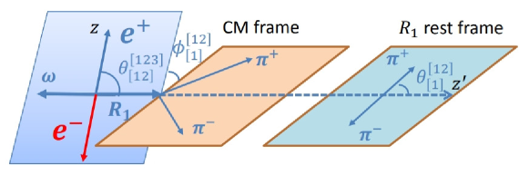
The amplitudes for these diagrams are constructed using the helicity formalism. Taking the first diagram in Fig. 2 as an example, one may define the helicity rotation angles as in Fig. 3. For resonance the polar angle () is defined as the angle spanned between the momentum and the positron beam direction, the azimuthal angle () is the angle between the production plane formed by the momentum and the axis and the plane formed by the and axes. Here, denotes the laboratory coordinates. The helicity amplitude for is denoted by with specified helicity and . For the decay, the azimuthal angle () is defined as the angle between the production plane and its decay plane, formed by the momenta of from . After boosting the two pion momenta to the rest frame, they are still located in the same decay plane. The polar angle () for is defined as the angle between the and momenta in the rest frame. The helicity amplitude of this decay is denoted by . Helicity angles for the processes (b) and (c) are defined analogously. Table 1 summarizes the helicity angles and amplitudes for the three processes.
| Process | Helicity angle | Helicity amplitude |
|---|---|---|
4.2 Decay amplitude
The decay amplitude for the process (a) is
| (1) |
where is the Wigner -function, is the spin quantum number of resonance , and denotes the Breit-Wigner function.
The decay amplitude for the process (b) is
| (2) | |||||
where is the spin of . Since the helicity defined in the helicity system is different from that defined in the process (a), one needs to perform a rotation by the angles () to align the helicity to coincide with that in the process (a). This issue has been addressed in the analyses lhcb ; belle and derived in detail in Ref. pingrg .
The decay amplitude for the process (c) reads
| (3) | |||||
where the Wigner function is used to align the helicity to coincide with that defined in the process (a).
For the direct three-body process , the helicity amplitude is written as chung2 :
| (4) |
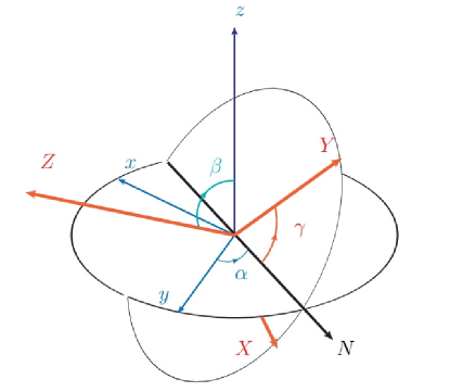
where is the component of the spin of the virtual photon in the helicity system, and is the helicity value for . Here, , , and are the Euler angles as defined in chung2 (see Fig. 4). is the helicity amplitude; parity conservation requires and . Parity conservation also requires and , where corresponds to the energy of the final state .
One usually expands the helicity amplitudes in terms of the partial waves for the two-body decay in the -coupling scheme chung2 . For a spin- particle decay , it follows
| (5) |
where and are the helicities of two final-state particles and with , and is a coupling constant, is the total spin , is the orbital angular momentum, , where is the relative momentum between the two daughter particles in their mother rest frame, corresponds to the value at the resonance’s known mass. is the Blatt-Weisskopf factor chung2 , which suppresses the contributions with higher angular momentum. The Blatt-Weisskopf factors up to = are
| (6) | |||||
where is a constant fixed to GeV-1 for the meson final states lhcb .
The differential cross section is given by
| (7) |
where due to the polarization of the virtual photon being produced from annihilation, and is the element of standard three-body PHSP. The is the decay matrix element into the final states, where is the polarization vector, and is the momentum vector for from the decay. Here we factor out the function describing the line shape into the MC integration when applying the amplitude analysis to the data events.
4.3 Simultaneous fit
The relative magnitudes and phases of the coupling constants are determined by an unbinned maximum likelihood fit. The joint probability density function (PDF) for the events observed in the data sample is defined as
| (8) |
where ( = , , …, ) denotes the four-vector momenta of the final state particles, and is a probability to produce the -th event. The normalized is calculated from the differential cross section
| (9) |
where is the normalization factor which is calculated with a large MC sample as
| (10) |
where is the number of events retained with the same selection criteria as for data sample.
For technical reasons, rather than maximizing , is minimized using the package MINUIT minuit . To subtract the contribution of background, the function is replaced with
| (11) |
where and are the joint PDFs for data and background, respectively. The background events are obtained from the sideband regions mentioned in Section 3.
A simultaneous fit is performed to data sets collected at different c.m. energies. The common parameters for different data samples in this fit are the masses, widths, and parameters for the resonances. The total function is taken as the sum of individual ones, ,
| (12) |
The signal yield for the -th resonance, , can be estimated by scaling its cross section ratio to the number of net events
| (13) |
where is the cross section for the -th resonance as defined in Eq.(7), is the total cross section, and and are the numbers of observed events and background events, respectively. In the simultaneous fit, the background events are taken from the sideband regions, and the number is estimated with the background PDF with the signal region (see Fig. 1).
The statistical uncertainty, , associated with the signal yield , is estimated according to the error propagation formula using the covariance matrix, , obtained in the simultaneous fit, i.e.
| (14) |
where is a vector containing parameters, and contains the fitted values for all parameters. The sum runs over all parameters.
4.4 Intermediate states in final state
In the and mass spectrum, the , , , , , , and resonances are included in the amplitude model. The line shape is parameterized by the formula:
| (15) |
where and is the momentum of the or in the resonance rest frame, and are fixed to the measured values and besiia ; besiib , respectively. is the mass of taken from the PDG pdg .
For the function of a wide resonance, e.g., , there are many parametrizations for the energy-dependent width besiia ; besiib , and we take the one used by the E791 Collaboration in the nominal fit,
| (16) |
where is the nominal mass of the resonance, and is its width. For other resonances, such as , , , , , their line shapes are described with the function,
| (17) |
where the widths are fixed to the individual PDG values pdg .
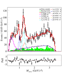
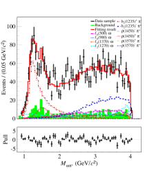
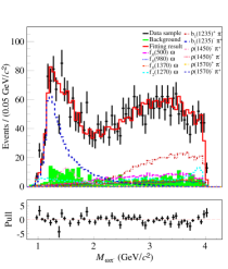
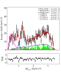
Based on the signal events in the mass spectrum, we select twelve c.m. energy points with relatively large statistics. We divide these selected points into two groups. Group A includes the data sets taken at = , , , , , and GeV, and group B includes = , , , , , and GeV. To check the significance of each resonance and determine the nominal solution, a simultaneous fit is performed to the data from a given group. In each group, the cross sections of these intermediate states are regarded to be energy-dependent, so the parameters responsible for the virtual photon coupling to a given state are allowed to vary in the fit for various energy points, while the coupling constant parameters for the subsequent decay are taken as the common parameters for all energies. The conjugate modes share the same coupling constants. The masses, widths or parameters for the resonances of , , , , , and are fixed to the measured values from PDG pdg , as given in Table 2. The mass and width of are floated due to large uncertainties. Then its nominal solution is fixed as the fitted result.
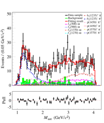
The significance of each intermediate state is estimated by the changes of and the number of degrees of freedom (NDF) after removing it from the simultaneous fit. We take the intermediate states with statistical significances greater than 5 in two groups as the nominal solution, including , , , , , and , as shown in Fig. 5. It is found that the contributions from and are the most significant, as shown in the and spectra, respectively. The statistical significances for various intermediate resonances are shown in Table 2.
| Resonance | Mass (MeV/) | Width (MeV) | Group A | Group B |
|---|---|---|---|---|
| 507 (400550) | 475 (400700) | 27.8 | 22.8 | |
| 10.9 | 6.4 | |||
| 1350150 | 20050 | 6.2 | 3.4 | |
| 9.3 | 5.4 | |||
| 31.8 | 25.7 | |||
| 1465.025 | 40060 | 4.7 | 6.9 | |
| 157070 | 14490 | 4.3 | 2.4 | |
| 6.5 | 3.0 |
4.5 Fit results
For the simultaneous fit, the ratios and the signal yields of various intermediate states are obtained according to Eq. (13), as shown in Tables 4 and 5. And their statistical uncertainties are determined based on Eq. (14), in which the correlation among parameters is included. With the intermediate states in the nominal solution, we perform the simultaneous fit to the data samples for groups A and B. Taking the two data samples from = and GeV with large integrated luminosity as examples, Figs. 5 and 6 show the fit results for groups A and B, respectively.
5 BORN CROSS SECTION
5.1 ISR correction factor
In collision experiments, the observed cross section, , at a c.m. energy point , is related to the corresponding Born cross section, , by the ISR factor
| (18) |
with
| (19) |
where is the vacuum polarization (VP) function. The corresponds to the mass threshold, and is the effective fraction of the beam energy carried by photons emitted from the initial state, , and is the energy of the ISR photons. The initial state radiative function, , which uses the QED calculation up to next to leading order in Ref wx ; alpha ; wsx ,
| (20) | ||||
where
| (21) |
and we use the calculated results including the leptonic and hadronic parts both in the space-like and time-like region isr11 ; isr12 ; isr13 ; isr14 ; isr15 .
We use the generator model ConExc besevtgen to produce signal MC events and then iterate the Born cross-section measurement, in which the radiative function takes the result of high-order QED calculation up to the accuracy alpha . The Born cross sections from the mass threshold to 4.6 GeV are used to calculate the ISR factor. The Born cross sections in the c.m. energy ranges of below GeV and GeV are taken from the measurements in Ref. babarXS and this work, respectively. In the c.m. energy interval of GeV, however, the Born cross section of continuum light hadrons is described by a polynomial, and the Born cross sections for and are described by the function
| (22) |
where is the c.m. energy, is the spin of the resonance, and the numbers of polarization states of the two incident particles are and , respectively. The maximum momentum of the final-state channel is denoted as , is the c.m. energy at the resonance, and is the width of the resonance. The branching fractions of the resonance decays into the initial-state and final-state channels are denoted as and , respectively. The cross sections are smoothed by a fit to seven Gaussian functions in various energy intervals. Since the detection efficiency is affected by the radiative correction, an iteration over the cross section is done until the latest two results become stable; specifically, when the updated Born cross sections change by less than the statistical uncertainty. The ISR correction factor for each c.m. energy point is given in Table 3.
5.2 Born cross section of
The Born cross section at each c.m. energy is calculated by
| (23) |
where is the number of observed signal events, and are the ISR correction and VP corrections, respectively. The factors and are the branching fractions of and from the PDG pdg . We use to denote the detection efficiency determined by the TOY MC sample with detector simulation of helicity amplitude model. The numerical results of Born cross sections are listed in Table 3.
| (GeV) | (pb) | |||||||
|---|---|---|---|---|---|---|---|---|
| 4.0076 | 482. | 0 | 634 | 28 | 4.5 | 1.0435 | ||
| 4.1285 | 393. | 4 | 408 | 23 | 4.6 | 1.0526 | ||
| 4.1574 | 406. | 9 | 398 | 22 | 4.8 | 1.0535 | ||
| 4.1780 | 3194. | 5 | 2888 | 60 | 4.8 | 1.0548 | ||
| 4.1890 | 523. | 9 | 452 | 24 | 4.8 | 1.0560 | ||
| 4.1990 | 525. | 2 | 462 | 26 | 4.9 | 1.0568 | ||
| 4.2093 | 517. | 2 | 467 | 24 | 4.8 | 1.0565 | ||
| 4.2188 | 513. | 4 | 444 | 24 | 4.9 | 1.0565 | ||
| 4.2263 | 1056. | 4 | 909 | 34 | 4.9 | 1.0548 | ||
| 4.2358 | 529. | 1 | 427 | 23 | 5.0 | 1.0554 | ||
| 4.2439 | 536. | 3 | 459 | 24 | 5.0 | 1.0552 | ||
| 4.2580 | 828. | 4 | 670 | 30 | 5.0 | 1.0533 | ||
| 4.2668 | 529. | 7 | 430 | 13 | 5.0 | 1.0531 | ||
| 4.2777 | 175. | 2 | 131 | 14 | 5.1 | 1.0529 | ||
| 4.2879 | 491. | 5 | 421 | 23 | 5.1 | 1.0525 | ||
| 4.3121 | 492. | 1 | 366 | 22 | 5.2 | 1.0519 | ||
| 4.3374 | 501. | 1 | 390 | 22 | 5.2 | 1.0508 | ||
| 4.3583 | 543. | 9 | 377 | 22 | 5.3 | 1.0511 | ||
| 4.3774 | 522. | 8 | 406 | 22 | 5.4 | 1.0514 | ||
| 4.3965 | 505. | 0 | 255 | 18 | 5.4 | 1.0517 | ||
| 4.4156 | 1043. | 9 | 716 | 30 | 5.4 | 1.0524 | ||
| 4.4362 | 568. | 1 | 365 | 21 | 5.5 | 1.0543 | ||
| 4.4671 | 111. | 1 | 80 | 10 | 5.6 | 1.0548 | ||
| 4.5995 | 586. | 9 | 259 | 18 | 6.1 | 1.0547 | ||
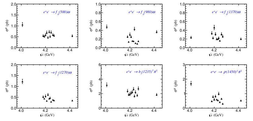
5.3 Born cross section for intermediate states
The Born cross section for each intermediate state is calculated by
| (24) |
where is the total Born cross section of , including the interference contributions among all intermediate states. The cross-section ratio, , is calculated according to Eq. (13) and given in Table 4, and the Born cross section of each intermediate state is shown in Fig. 7.
| Group | (GeV) | |||||||
|---|---|---|---|---|---|---|---|---|
| 4.0076 | ||||||||
| 4.1780 | ||||||||
| A | 4.1890 | |||||||
| 4.1990 | ||||||||
| 4.2093 | ||||||||
| 4.2188 | ||||||||
| 4.2263 | ||||||||
| 4.2358 | ||||||||
| B | 4.2439 | |||||||
| 4.2580 | ||||||||
| 4.2668 | ||||||||
| 4.4156 |
| Group | (GeV) | ||||||||||||
|---|---|---|---|---|---|---|---|---|---|---|---|---|---|
| 4.0076 | 77.40 | 13.51 | 34.88 | 12.36 | 17.21 | 12.15 | 89.32 | 15.50 | 233.49 | 26.19 | 123.89 | 23.47 | |
| 4.1780 | 298.92 | 28.95 | 136.22 | 29.90 | 179.80 | 40.13 | 281.23 | 37.93 | 1284.20 | 63.06 | 260.12 | 42.96 | |
| A | 4.1890 | 47.14 | 10.67 | 12.28 | 11.92 | 20.31 | 13.80 | 39.90 | 13.47 | 170.09 | 19.53 | 71.91 | 17.73 |
| 4.1990 | 53.41 | 11.19 | 27.73 | 14.27 | 42.27 | 16.92 | 50.58 | 15.52 | 176.50 | 19.13 | 54.62 | 16.57 | |
| 4.2093 | 59.40 | 12.32 | 21.34 | 11.31 | 26.77 | 17.14 | 28.84 | 13.23 | 180.88 | 19.48 | 70.47 | 19.60 | |
| 4.2188 | 42.73 | 10.00 | 13.99 | 9.97 | 17.97 | 13.92 | 56.45 | 13.82 | 203.56 | 22.39 | 54.25 | 19.80 | |
| 4.2263 | 128.26 | 17.67 | 26.69 | 12.74 | 34.71 | 18.75 | 77.60 | 17.80 | 466.33 | 33.06 | 95.40 | 24.50 | |
| 4.2358 | 47.61 | 12.54 | 39.58 | 13.21 | 20.56 | 15.28 | 43.47 | 10.32 | 153.61 | 20.45 | 92.14 | 19.50 | |
| B | 4.2439 | 68.69 | 11.56 | 9.99 | 7.78 | 15.42 | 11.29 | 28.71 | 11.16 | 214.59 | 20.95 | 41.08 | 18.88 |
| 4.2580 | 81.67 | 15.42 | 12.52 | 8.91 | 43.09 | 16.44 | 53.24 | 14.53 | 246.22 | 24.71 | 89.86 | 21.01 | |
| 4.2668 | 49.34 | 11.15 | 13.15 | 8.74 | 22.76 | 16.21 | 31.61 | 13.65 | 237.85 | 26.53 | 27.10 | 18.16 | |
| 4.4156 | 96.94 | 16.25 | 64.90 | 20.71 | 35.83 | 26.22 | 62.95 | 17.77 | 334.32 | 28.10 | 94.23 | 24.30 | |
6 SYSTEMATIC UNCERTAINTY
6.1 Uncertainty of the Born cross section
The uncertainties in the Born cross section measurements arise from the luminosity measurement, tracking and PID efficiency, photon detection efficiency, branching fraction, veto, ISR correction, fit procedure, PWA, and insignificant resonances. However, the effects of the requirement and veto on efficiency are negligible.
-
•
Luminosity. The integrated luminosity is measured by the Bhabha scattering process, and the uncertainty is % rlum .
-
•
Tracking and PID efficiencies. The uncertainty of the tracking efficiency has been studied with a high purity control sample of prd1012003 . The differences of the tracking and PID efficiencies between data and MC simulation in different transverse momentum and momentum ranges are taken as the systematic uncertainties of tracking and PID efficiencies, both % per charged pion.
-
•
Photon detection efficiency. The uncertainty from the photon detection has been studied with the control samples of and prd1012003 , which is % per photon.
-
•
Branching fraction. The branching fractions and are quoted from the PDG pdg , which are ()% and ()%, respectively. The relevant systematic uncertainty is % in total.
-
•
veto. The uncertainty of veto is taken as the difference of efficiencies with and without veto between data and MC simulation, which is %.
-
•
ISR correction. To obtain reliable detection efficiencies, the Born cross sections input in the generator have been iterated until the values converge. The differences of between the last two iterations are taken as the corresponding systematic uncertainties.
-
•
Fit procedure. The systematic uncertainty in the fit of mainly comes from the fit range, signal shape and background shape. The fit range is changed from [, ] GeV/ to [, ] GeV/. The signal shape is changed to the function convolved with a Gaussian resolution function. The background shape is changed from the second-order Chebyshev polynomial to the third-order, and the parameter of the background function is fixed to that derived from the fit to the largest data sample taken at GeV. The quadrature sum of the changes in the fitted signal yield is taken as the uncertainty.
-
•
PWA. The uncertainties due to the mass and width of the intermediate resonance state, the background level, and the kinematic fit are considered in the systematic uncertainty of PWA. The main contribution comes from , , , , and . The total uncertainty is the sum of the following three detailed sources.
-
•
Mass and width. The masses and widths of the intermediate resonance states in this analysis are fixed on the PDG values pdg . To estimate their systematic uncertainties, we shift the mass and width of each intermediate resonance within one standard deviation.
-
•
Background level. The background level is determined by the sideband events of the data sample. It is the same size as the number of events obtained in the signal region after the integration of the background function. To estimate the systematic uncertainty of the background level, we determine the deviation of the background level according to , where is the estimated number of the background events in the signal region, and change the background yield by ().
-
•
Kinematic fit. The uncertainty of the kinematic fit is estimated by correcting the helix parameters of the charged tracks to improve the consistency between data and MC simulation prd012002 . The difference in the detection efficiencies of the TOY MC samples is regarded as the systematic uncertainty in PWA.
-
•
Insignificant resonance. An intermediate state with significance less than , , is removed in the normal solution. The uncertainty is defined as the difference between the detection efficiencies of the normal solution with and without the contribution.
The numerical values of these systematic uncertainties are summarized in Table 6. For the total uncertainty these contributions are added in quadrature.
6.2 Uncertainty of the Born cross section for intermediate process
The systematic uncertainty in the measurements of the Born cross sections for the intermediate processes is the same as that of . Whereas, for the Born cross section measurement of intermediate state, the uncertainty in PWA depends on the ratio of each intermediate state, . We mainly estimate the systematic uncertainty of the Born cross section of different intermediate processes for the twelve c.m. energy points with higher statistics. Their uncertainties are obtained by adding the individual contributions in quadrature and summarized in Table 7.
-
•
Mass and width. For the uncertainties of the mass and width of any of the intermediate resonance states, we change its mass and width according to the PDG values within .
-
•
Background level. We determine the deviation of the background level according to , and change the background yield to obtain the uncertainty of the background level.
-
•
Kinematic fit. We use the PHSP signal MC sample corrected by the helix parameters to re-perform PWA to estimate the uncertainty of the kinematic fit.
-
•
Insignificant resonance. The uncertainty due to one insignificant resonance was defined as the difference between the ratio of the normal solution with and without the contribution.
For each source, the deviation from the nominal result is taken as the corresponding systematic uncertainty.
| (GeV) | ∗ | ISR | SS | BS | FR | PWA | IR | Total | |||||
|---|---|---|---|---|---|---|---|---|---|---|---|---|---|
| 4.0076 | 1.0 | 4.0 | 4.0 | 2.0 | 0.75 | 0.8 | 1.1 | 0.8 | 1.1 | 0.6 | 0.3 | 3.1 | 7.2 |
| 4.1285 | 1.0 | 4.0 | 4.0 | 2.0 | 0.75 | 0.8 | 2.8 | 0.7 | 0.7 | 1.0 | 0.2 | 4.1 | 8.1 |
| 4.1574 | 1.0 | 4.0 | 4.0 | 2.0 | 0.75 | 0.8 | 1.5 | 1.0 | 1.5 | 0.0 | 4.8 | 0.4 | 8.2 |
| 4.1780 | 1.0 | 4.0 | 4.0 | 2.0 | 0.75 | 0.8 | 5.2 | 0.6 | 1.1 | 0.7 | 0.0 | 1.7 | 8.4 |
| 4.1890 | 1.0 | 4.0 | 4.0 | 2.0 | 0.75 | 0.8 | 0.7 | 0.9 | 0.7 | 0.0 | 3.5 | 3.0 | 7.8 |
| 4.1990 | 1.0 | 4.0 | 4.0 | 2.0 | 0.75 | 0.8 | 5.5 | 0.0 | 1.5 | 0.7 | 2.6 | 4.6 | 10.0 |
| 4.2093 | 1.0 | 4.0 | 4.0 | 2.0 | 0.75 | 0.8 | 3.9 | 0.6 | 0.9 | 1.2 | 2.7 | 2.6 | 8.3 |
| 4.2188 | 1.0 | 4.0 | 4.0 | 2.0 | 0.75 | 0.8 | 1.0 | 0.7 | 0.9 | 1.1 | 1.7 | 5.8 | 8.9 |
| 4.2263 | 1.0 | 4.0 | 4.0 | 2.0 | 0.75 | 0.8 | 0.6 | 0.3 | 1.3 | 0.4 | 1.3 | 3.9 | 7.6 |
| 4.2358 | 1.0 | 4.0 | 4.0 | 2.0 | 0.75 | 0.8 | 3.6 | 0.2 | 0.9 | 1.9 | 2.1 | 2.9 | 8.3 |
| 4.2439 | 1.0 | 4.0 | 4.0 | 2.0 | 0.75 | 0.8 | 1.5 | 0.7 | 1.1 | 0.7 | 0.8 | 3.1 | 7.3 |
| 4.2580 | 1.0 | 4.0 | 4.0 | 2.0 | 0.75 | 0.8 | 0.8 | 1.4 | 1.5 | 1.1 | 2.7 | 1.4 | 7.3 |
| 4.2668 | 1.0 | 4.0 | 4.0 | 2.0 | 0.75 | 0.8 | 1.1 | 0.2 | 1.2 | 0.0 | 1.5 | 4.0 | 7.7 |
| 4.2777 | 1.0 | 4.0 | 4.0 | 2.0 | 0.75 | 0.8 | 4.7 | 0.0 | 1.5 | 0.0 | 1.5 | 4.6 | 9.3 |
| 4.2879 | 1.0 | 4.0 | 4.0 | 2.0 | 0.75 | 0.8 | 2.7 | 0.5 | 1.0 | 0.5 | 0.2 | 1.0 | 6.9 |
| 4.3121 | 1.0 | 4.0 | 4.0 | 2.0 | 0.75 | 0.8 | 5.9 | 0.6 | 1.6 | 1.1 | 0.9 | 5.0 | 10.1 |
| 4.3374 | 1.0 | 4.0 | 4.0 | 2.0 | 0.75 | 0.8 | 6.8 | 1.0 | 0.5 | 0.5 | 3.0 | 1.1 | 9.8 |
| 4.3583 | 1.0 | 4.0 | 4.0 | 2.0 | 0.75 | 0.8 | 3.2 | 1.1 | 1.3 | 1.6 | 1.1 | 2.5 | 7.8 |
| 4.3774 | 1.0 | 4.0 | 4.0 | 2.0 | 0.75 | 0.8 | 0.0 | 0.5 | 1.0 | 1.5 | 0.2 | 0.5 | 6.5 |
| 4.3965 | 1.0 | 4.0 | 4.0 | 2.0 | 0.75 | 0.8 | 2.9 | 0.4 | 0.8 | 0.0 | 2.0 | 1.2 | 7.3 |
| 4.4156 | 1.0 | 4.0 | 4.0 | 2.0 | 0.75 | 0.8 | 1.4 | 0.3 | 0.8 | 0.9 | 1.7 | 3.2 | 7.4 |
| 4.4362 | 1.0 | 4.0 | 4.0 | 2.0 | 0.75 | 0.8 | 5.5 | 0.8 | 1.1 | 0.8 | 3.3 | 0.1 | 9.0 |
| 4.4671 | 1.0 | 4.0 | 4.0 | 2.0 | 0.75 | 0.8 | 3.8 | 0.0 | 1.3 | 1.3 | 2.8 | 5.6 | 9.7 |
| 4.5995 | 1.0 | 4.0 | 4.0 | 2.0 | 0.75 | 0.8 | 1.6 | 0.8 | 1.1 | 1.6 | 3.0 | 2.4 | 7.7 |
| Group | (GeV) | ||||||
|---|---|---|---|---|---|---|---|
| 4.0076 | 7.9 | 7.1 | 9.1 | 7.2 | 7.2 | 7.1 | |
| 4.1780 | 8.5 | 8.3 | 10.3 | 8.3 | 8.3 | 8.2 | |
| A | 4.1890 | 7.0 | 6.5 | 9.4 | 6.5 | 6.5 | 6.4 |
| 4.1990 | 8.7 | 8.7 | 10.1 | 8.7 | 8.7 | 8.6 | |
| 4.2093 | 7.7 | 7.5 | 9.3 | 7.5 | 7.6 | 7.5 | |
| 4.2188 | 7.2 | 6.9 | 9.0 | 6.9 | 6.9 | 6.8 | |
| 4.2263 | 6.9 | 6.6 | 8.4 | 6.6 | 6.6 | 6.5 | |
| 4.2358 | 7.9 | 7.7 | 9.6 | 7.7 | 7.7 | 7.6 | |
| B | 4.2439 | 7.3 | 6.6 | 8.9 | 6.6 | 6.7 | 6.6 |
| 4.2580 | 7.3 | 6.7 | 9.3 | 6.6 | 6.7 | 6.8 | |
| 4.2668 | 8.5 | 7.5 | 10.2 | 7.5 | 7.6 | 7.9 | |
| 4.4156 | 7.6 | 6.9 | 9.2 | 6.8 | 6.9 | 7.1 |
7 FIT TO THE LINE SHAPE
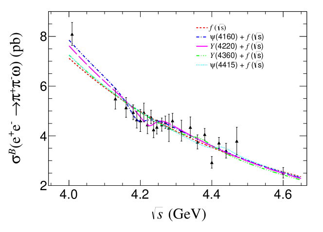
The line shape for total Born cross section of is fitted with the least square method leastchi2 . First, the energy-dependent Born cross section is parameterized by a non-resonant function , where and are free parameters. The correlations among different c.m. energy points are considered in the fit with the defined as below (and minimized by MINUIT minuit ),
| (25) |
where and are the measured and fitted values for Born cross section at the -th c.m. energy point, respectively. here, is the uncertainty for the -th c.m. energy point, which includes the statistical uncertainty and the uncorrelated part of the systematic uncertainty. Figure 8 shows the fit result with .
Secondly, the Born cross section is parameterized as the coherent sum of the energy-dependent non-resonant function and one charmonium or charmonium-like state amplitude,
| (26) |
where denotes the non-resonant amplitude, is the relative phase between the continuum and resonant amplitudes, and is a relativistic function which is used to describe the charmonium states, . And since these energies are far from the threshold of the process, the effect of the three-body phase space factor is very small and therefore this function omits it. The symbols , , , and denote the mass, the branching fraction of , the partial width to , and the total width, respectively. The considered charmonium and charmonium-like states include , , , and . In the fit, these resonance states are individually fitted with fixed mass and width from the PDG. The fit results are shown in Fig. 8. The goodness-of-fit tests for , , , and yield , , , and , respectively. The fit has two solutions with equal fit quality. The fitted parameters of various resonance states are shown in Table 8. The statistical significances of and are and , while those of and are and , respectively.
| Parameter | ||||
|---|---|---|---|---|
| Solution I | Solution II | Solution I | Solution II | |
| (eV) | ||||
| 0.070 | 0.055 | |||
| M | 4.191 | 4.23 | ||
| (rad) | ||||
| Significance () | 3.6 | 3.1 | ||
8 SUMMARY
In conclusion, the process of is studied at twenty-four c.m. energies in the region from to GeV. The Born cross sections of and the intermediate state production at twelve c.m. energy points are measured with helicity amplitude analysis method. The results indicate that the dominant contributions are from , , , , , with statistical significances greater than . By analyzing the line shape of the Born cross section of the process, greater than evidence for a state with mass about GeV/ is found, which is consistent with the production of either or .
Acknowledgements.
The BESIII collaboration thanks the staff of BEPCII and the IHEP computing center for their strong support. This work is supported in part by National Key R&D Program of China under Contracts Nos. 2020YFA0406300, 2020YFA0406400; National Natural Science Foundation of China (NSFC) under Contracts Nos. 11975118, 12175244, 11875262, 11635010, 11735014, 11835012, 11935015, 11935016, 11935018, 11961141012, 12022510, 12025502, 12035009, 12035013, 12192260, 12192261, 12192262, 12192263, 12192264, 12192265, 12061131003; the Science and Technology Innovation Program of Hunan Province under Contract No. 2020RC3054; the Chinese Academy of Sciences (CAS) Large-Scale Scientific Facility Program; Joint Large-Scale Scientific Facility Funds of the NSFC and CAS under Contract No. U1832207; the CAS Center for Excellence in Particle Physics (CCEPP); 100 Talents Program of CAS; The Institute of Nuclear and Particle Physics (INPAC) and Shanghai Key Laboratory for Particle Physics and Cosmology; ERC under Contract No. 758462; European Union’s Horizon 2020 research and innovation programme under Marie Sklodowska-Curie grant agreement under Contract No. 894790; German Research Foundation DFG under Contracts Nos. 443159800, Collaborative Research Center CRC 1044, GRK 2149; Istituto Nazionale di Fisica Nucleare, Italy; Ministry of Development of Turkey under Contract No. DPT2006K-120470; National Science and Technology fund; National Science Research and Innovation Fund (NSRF) via the Program Management Unit for Human Resources & Institutional Development, Research and Innovation under Contract No. B16F640076; STFC (United Kingdom); Suranaree University of Technology (SUT), Thailand Science Research and Innovation (TSRI), and National Science Research and Innovation Fund (NSRF) under Contract No. 160355; The Royal Society, UK under Contracts Nos. DH140054, DH160214; The Swedish Research Council; U. S. Department of Energy under Contract No. DE-FG02-05ER41374References
- (1) P.A. Zyla et al. [Particle Data Group], Review of Particle Physics, Prog. Theor. Exp. Phys. 2020 (2020) 083C01.
- (2) S.K. Choi et al. [Belle Collaboration], Observation of a narrow charmonium-like state in exclusive decays, Phys. Rev. Lett. 91 (2003) 262001 [arXiv:hep-ex/0309032] [INSPIRE].
- (3) B. Aubert et al. [BaBar Collaboration], Observation of a Broad Structure in the Mass Spectrum around 4.26 GeV/, Phys. Rev. Lett. 95 (2005) 142001 [arXiv:hep-ex/0506081] [INSPIRE].
- (4) M. Ablikim et al. [BESIII Collaboration], Observation of a Charged Charmoniumlike Structure in at =4.26 GeV, Phys. Rev. Lett. 110 (2013) 252001 [arXiv:1303.5949] [INSPIRE].
- (5) S.K. Choi et al. [Belle Collaboration], Study of and Observation of a Charged Charmoniumlike State at Belle, Phys. Rev. Lett. 110 (2013) 252002 [arXiv:1304.0121] [INSPIRE].
- (6) Q. He et al. [CLEO Collaboration], Confirmation of the Y(4260) resonance production in ISR, Phys. Rev. D 74 (2006) 091104 [arXiv:hep-ex/0611021] [INSPIRE].
- (7) C. Z. Yuan et al. [Belle Collaboration], Measurement of cross-section via initial state radiation at Belle, Phys. Rev. Lett. 99 (2007) 182004 [arXiv:0707.2541] [INSPIRE].
- (8) M. Ablikim et al. [BESIII Collaboration], Precise Measurement of the Cross Section at Center-of-Mass Energies from 3.77 to 4.60 GeV, Phys. Rev. Lett. 118 (2017) 092001 [arXiv:1611.01317] [INSPIRE].
- (9) M. Ablikim et al. [BESIII Collaboration], Study of at center-of-mass energies from 4.21 to 4.42 GeV, Phys. Rev. Lett. 114 (2015) 092003 [arXiv:1410.6538] [INSPIRE].
- (10) M. Ablikim et al. [BESIII Collaboration], Evidence of Two Resonant Structures in , Phys. Rev. Lett. 118 (2017) 092002 [arXiv:1610.07044] [INSPIRE].
- (11) M. Ablikim et al. [BESIII Collaboration], Measurement of from 4.008 to 4.600 GeV and observation of a charged structure in the mass spectrum, Phys. Rev. D 96 (2017) 032004 [arXiv:1703.08787] [INSPIRE].
- (12) M. Ablikim et al. [BESIII Collaboration], Evidence of a resonant structure in the cross section between 4.05 and 4.60 GeV, Phys. Rev. Lett. 122 (2019) 102002 [arXiv:1808.02847] [INSPIRE].
- (13) B. Aubert et al. [BaBar Collaboration], Evidence of a broad structure at an invariant mass of 4.32 GeV/ in the reaction measured at BaBar, Phys. Rev. Lett. 98 (2007) 212001 [arXiv:hep-ex/0610057] [INSPIRE].
- (14) S.K. Choi et al. [Belle Collaboration], Observation of Two Resonant Structures in via Initial State Radiation at Belle, Phys. Rev. Lett. 99 (2007) 142002 [arXiv:0707.3699] [INSPIRE].
- (15) H. X. Chen et al., The hidden-charm pentaquark and tetraquark states, Phys. Rept. 639 (2016) 1 [arXiv:1601.02092] [INSPIRE].
- (16) Y. R. Liu et al., Pentaquark and Tetraquark states, Prog. Part. Nucl. Phys. 107 (2019) 237 [arXiv:1903.11976] [INSPIRE].
- (17) L. Maiani et al., Four quark interpretation of Y(4260), Phys. Rev. D 72 (2005) 031502 [arXiv:hep-ph/0507062] [INSPIRE].
- (18) A. Ali et al., A new look at the Y tetraquarks and baryons in the diquark model, Eur. Phys. J. C 78 (2018) 29 [arXiv:1708.04650] [INSPIRE].
- (19) S.J. Brodsky et al., A New Picture for the Formation and Decay of the Exotic XYZ Mesons, Phys. Rev. Lett. 113 (2014) 112001 [arXiv:1406.7281] [INSPIRE].
- (20) J.R. Zhang and M.Q. Huang, The P-wave tetraquark state: Y(4260) or Y(4660)?, Phys. Rev. D 83 (2011) 036005 [arXiv:1011.2818] [INSPIRE].
- (21) J.R. Zhang and M.Q. Huang, Could (10890) be the P-wave tetraquark state?, JHEP 11 (2010) 057 [arXiv:1011.2815] [INSPIRE].
- (22) Z.G. Wang, Tetraquark state candidates: Y(4260), Y(4360), Y(4660) and (4020/4025), Eur. Phys. J. C 76 (2016) 387 [arXiv:1601.05541] [INSPIRE].
- (23) N. Brambilla et al., Heavy quarkonium: progress, puzzles, and opportunities, Eur. Phys. J. C 71 (2011) 1534 [arXiv:arXiv:1010.5827] [INSPIRE].
- (24) S.L. Zhu, The Possible interpretations of Y(4260), Phys. Lett. B 625 (2005) 212 [arXiv:hep-ph/0507025] [INSPIRE].
- (25) F.E. Close and P.R. Page, Gluonic charmonium resonances at BaBar and BELLE?, Phys. Lett. B 628 (2005) 215 [arXiv:hep-ph/0507199] [INSPIRE].
- (26) L. Liu et al., Excited and exotic charmonium spectroscopy from lattice QCD, JHEP 07 (2012) 126 [arXiv:1204.5425] [INSPIRE].
- (27) E. Braaten et al., Born-Oppenheimer Approximation for the XYZ Mesons, Phys. Rev. D 90 (2014) 014044 [arXiv:1402.0438] [INSPIRE].
- (28) X. Li and M.B. Voloshin, Y(4260) and Y(4360) as mixed hadrocharmonium, Mod. Phys. Lett. A 29 (2014) 1450060 [arXiv:1309.1681] [INSPIRE].
- (29) M.B. Voloshin, Charmonium, Prog. Part. Nucl. Phys. 61 (2008) 455 [arXiv:0711.4556] [INSPIRE].
- (30) F.K. Guo et al., Evidence that the Y(4660) is an bound state, Phys. Lett. B 665 (2008) 26 [arXiv:0803.1392] [INSPIRE].
- (31) Z.G. Wang and X.H. Zhang, Analysis of Y(4660) and related bound states with QCD sum rules, Commun. Theor. Phys. 54 (2010) 323 [arXiv:0905.3784] [INSPIRE].
- (32) Q. Wang et al., Decoding the riddle of Y(4260) and (3900), Phys. Rev. Lett. 111 (2013) 132003 [arXiv:1303.6355] [INSPIRE].
- (33) M. Cleven et al., Y(4260) as the first S-wave open charm vector molecular state?, Phys. Rev. D 90 (2014) 074039 [arXiv:1310.2190] [INSPIRE].
- (34) Q. Wang et al., Y(4260): hadronic molecule versus hadro-charmonium interpretation, Phys. Rev. D 89 (2014) 034001 [arXiv:1309.4303] [INSPIRE].
- (35) Z.G. Wang, Analysis of the Y(4220) and Y(4390) as molecular states with QCD sum rules, Chin. Phys. C 41 (2017) 083103 [arXiv:1611.03250] [INSPIRE].
- (36) D.Y. Chen et al., Nonresonant explanation for the Y(4260) structure observed in the process, Phys. Rev. D 83 (2011) 054021 [arXiv:1012.5362] [INSPIRE].
- (37) D.Y. Chen et al., Unified Fano-like interference picture for charmoniumlike states Y(4008), Y(4260) and Y(4360), Phys. Rev. D 93 (2016) 014011 [arXiv:1512.04157] [INSPIRE].
- (38) A. Martinez Torres et al., The Y(4260) as a system, Phys. Rev. D 80 (2009) 094012 [arXiv:0906.5333] [INSPIRE].
- (39) X.H. Liu and G. Li, Exploring the threshold behavior and implications on the nature of Y(4260) and (3900), Phys. Rev. D 88 (2013) 014013 [arXiv:1306.1384] [INSPIRE].
- (40) C.F. Qiao, One explanation for the exotic state Y(4260), Phys. Lett. B 639 (2006) 263 [arXiv:hep-ph/0510228] [INSPIRE].
- (41) R. Brandelik et al. [DASP Collaboration], Total Cross-section for Hadron Production by Annihilation at Center-of-mass Energies Between 3.6 and 5.2 GeV , Phys. Lett. B 76 (1978) 361 [INSPIRE].
- (42) M. Ablikim et al. [BES Collaboration], Determination of the (3770), (4040), (4160) and (4415) resonance parameters, Phys. Lett. B 660 (2008) 315 [arXiv:0705.4500] [INSPIRE].
- (43) X.H. Mo et al., On the leptonic partial widths of the excited states, Phys. Rev. D 82 (2010) 077501 [arXiv:1007.0084] [INSPIRE].
- (44) R. Aaij et al. [LHCb Collaboration], Observation of a resonance in decays at low recoil, Phys. Rev. Lett. 111 (2013) 112003 [arXiv:1307.7595] [INSPIRE].
- (45) M. Ablikim et al. [BESIII Collaboration], Measurements of and at center-of-mass energies from 3.90 to 4.60 GeV, Phys. Rev. D 99 (2019) 012003 [arXiv:1810.09395] [INSPIRE].
- (46) M. Ablikim et al. [BESIII Collaboration], Precision measurements of at center-of-mass energies between 3.8 and 4.6 GeV, Phys. Rev. D 99 (2019) 072005 [arXiv:1808.08733] [INSPIRE].
- (47) M. Ablikim et al. [BESIII Collaboration], Study of at center-of-mass energies between 4.0 and 4.6 GeV, Phys. Rev. D 103 (2021) 052003 [arXiv:2012.11079] [INSPIRE].
- (48) M. Ablikim et al. [BESIII Collaboration], Cross sections for the reactions in the energy region between 3.773 and 4.600 GeV, Phys. Rev. D 104 (2021) 112009.
- (49) M. Ablikim et al. [BESIII Collaboration], Search for , Phys. Rev. D 92 (2015) 032009 [arXiv:1507.02068] [INSPIRE].
- (50) M. Ablikim et al. [BESIII Collaboration], Design and Construction of the BESIII Detector, Nucl. Instrum. Meth. A 614 (2010) 345 [arXiv:0911.4960] [INSPIRE].
- (51) C. H. Yu et al., BEPCII Performance and Beam Dynamics Studies on Luminosity, Proceedings of IPAC2016, Busan, Korea, 2016 [INSPIRE].
- (52) K. X. Huang, et al., Method for detector description transformation to Unity and application in BESIII, Nucl. Sci. Tech. 33, (2022) 142.
- (53) X. Li et al., Study of MRPC technology for BESIII endcap-TOF upgrade, Radiat. Detect. Technol. Methods 1 (2017) 13; Y. X. Guo et al., The study of time calibration for upgraded end cap TOF of BESIII, Radiat. Detect. Technol. Methods 1 (2017) 15; P. Cao et al., Design and construction of the new BESIII endcap Time-of-Flight system with MRPC Technology, Nucl. Instrum. Meth. A 953 (2020) 163053.
- (54) M. Ablikim et al. [BESIII Collaboration], Measurement of the center-of-mass energies at BESIII via the di-muon process, Chin. Phys. C 40 (2016) 063001 [arXiv:1510.08654] [INSPIRE]; Y.F. Yang et al. [BESIII Collaboration], BAM-00340; A. Juli and A. Gilman et al. [BESIII Collaboration], BESIII-DOC 580.
- (55) M. Ablikim et al. [BESIII Collaboration], Precision measurement of the integrated luminosity of the data taken by BESIII at center of mass energies between 3.810 GeV and 4.600 GeV, Chin. Phys. C 39 (2015) 093001 [arXiv:1503.03408] [INSPIRE]; Y.F. Yang et al. [BESIII Collaboration], BAM-00340.
- (56) Z. Y. Deng et al., Object-Oriented BESIII Detector Simulation System, Chin. Phys. C 30 (2006) 371.
- (57) S. Agostinelli et al., [GEANT4 Collaboration], GEANT4–a simulation toolkit, Nucl. Instrum. Meth. A 506 (2003) 250 [INSPIRE].
- (58) Y. T. Liang et al., A uniform geometry description for simulation, reconstruction and visualization in the BESIII experiment, Nucl. Instrum. Meth. A 603 (2009) 325 [INSPIRE].
- (59) Z. Y. You et al., A method for detector description exchange among ROOT GEANT4 and GEANT3, Chin. Phys. C 32 (2008) 572.
- (60) S. Jadach et al., The Precision Monte Carlo event generator KK for two fermion final states in collisions, Comput. Phys. Commun. 130, 260 (2000) [arXiv:hep-ph/9912214] [INSPIRE]; S. Jadach et al., Coherent exclusive exponentiation for precision Monte Carlo calculations, Phys. Rev. D 63 (2001) 113009 [arXiv:hep-ph/0006359] [INSPIRE].
- (61) R. G. Ping, Event generators at BESIII, Chin. Phys. C 32 (2008) 599 [INSPIRE]; D. J. Lange, The EvtGen particle decay simulation package, Nucl. Instr. Meth. A 462 (2001) 152 [INSPIRE].
- (62) M. Ablikim et al. [BESII Collaboration], Cross section measurements of from =4.178 to 4.278 GeV, Phys. Rev. D 99 (2019) 091103 [arXiv:1903.02359] [INSPIRE].
- (63) R. Aaij et al. [LHCb Collaboration], Observation of Resonances Consistent with Pentaquark States in Decays, Phys. Rev. Lett. 115 (2015) 072001 [arXiv:1507.03414] [INSPIRE].
- (64) K. Chilikin et al. [Belle Collaboration], Experimental constraints on the spin and parity of the , Phys. Rev. D 88 (2013) 074026 [arXiv:1306.4894] [INSPIRE].
- (65) H. Chen and R. G. Ping, Coherent helicity amplitude for sequential decays, Phys. Rev. D 95 (2017) 076010 [arXiv:1704.05184] [INSPIRE].
- (66) S. U. Chung, A General formulation of covariant helicity coupling amplitudes, Phys. Rev. D 57 (1998) 431 [INSPIRE]; S. U. Chung, Helicity coupling amplitudes in tensor formalism, Phys. Rev. D 48 (1993) 1225 [INSPIRE]; S. U. Chung and J. M. Friedrich, Covariant helicity-coupling amplitudes: A New formulation, Phys. Rev. D 78 (2008) 074027 [arXiv:0711.3143] [INSPIRE].
- (67) F. James, Minuit: A System for Function Minimization and Analysis of the Parameter Errors and Correlations, Comput. Phys. Commun. 10 (1975) 343 [INSPIRE].
- (68) M. Ablikim et al. [BESII Collaboration], The sigma pole in , Phys. Lett. B 598 (2004) 149 [arXiv:hep-ex/0406038] [INSPIRE].
- (69) M. Ablikim et al. [BESII Collaboration], Production of sigma in , Phys. Lett. B 645 (2007) 19 [arXiv:hep-ex/0610023] [INSPIRE].
- (70) V. P. Druzhinin, S. I. Eidelman, S. I. Serednyakov, and E. P. Solodov, Hadron production via collisions with initial state radiation, Rev. Mod. Phys. 83 (2011) 1545 [arXiv:hep-ph/1105.4975] [INSPIRE].
- (71) E. A. Kuraev, and V. S. Fadin, On Radiative Corrections to Single Photon Annihilation at High-Energy, Sov. J. Nucl. Phys. 41 (1985) 466-472 [INSPIRE].
- (72) R. G. Ping et al., Tuning and validation of hadronic event generator for R value measurements in the tau-charm region, Chinese Phys. C 40 (2016) 113002
- (73) S. Eidelman and F. Jegerlehner, Hadronic contributions to (g-2) of the leptons and to the effective fine structure constant , Z. Phys. C 67 (1995) 585 [arXiv:hep-ph/9502298] [INSPIRE].
- (74) F. Jegerlehner, Precision measurements of for at ILC energies and , Nucl. Phys. B 162 (2006) 22 [arXiv:hep-ph/0608329] [INSPIRE].
- (75) F. Jegerlehner, The Running fine structure constant via the Adler function, Nucl. Phys. B Proc. Suppl. 181 (2008) 135 [arXiv:0807.4206] [INSPIRE].
- (76) F. Jegerlehner, Theoretical precision in estimates of the hadronic contributions to and , Nucl. Phys. B Proc. Suppl. 126 (2004) 325 [arXiv:hep-ph/0310234] [INSPIRE].
- (77) F. Jegerlehner, Hadronic vacuum polarization effects in , Mini-Workshop on Electroweak Precision Data and the Higgs Mass, (2003) 97 [arXiv:hep-ph/0308117] [INSPIRE].
- (78) B. Aubert et al. [Babar Collaboration], The and Cross Sections Measured with Initial-State Radiation, Phys. Rev. D 76 (2007) 092005 [arXiv:0708.2461] [INSPIRE].
- (79) M. Ablikim et al. [BESIII Collaboration], Measurements of the branching fractions of and , Phys. Rev. D 100 (2019) 012003 [arXiv:1903.05375] [INSPIRE].
- (80) M. Ablikim et al. [BESIII Collaboration], Search for hadronic transition and observation of , Phys. Rev. D 87 (2013) 012002 [arXiv:1208.4805] [INSPIRE].
- (81) B. P. Roe, Probability and Statistics in Experimental Physics, 2nd edn., New York (2001).
- (82) X. H. Mo, Unbiased Estimator for Linear Function Fit Involving Correlated Data, HEPNP 31 (2007) 745.
M. Ablikim1, M. N. Achasov11,b, P. Adlarson70, M. Albrecht4, R. Aliberti31, A. Amoroso69A,69C, M. R. An35, Q. An66,53, Y. Bai52, O. Bakina32, R. Baldini Ferroli26A, I. Balossino27A, Y. Ban42,g, V. Batozskaya1,40, D. Becker31, K. Begzsuren29, N. Berger31, M. Bertani26A, D. Bettoni27A, F. Bianchi69A,69C, E. Bianco69A,69C, J. Bloms63, A. Bortone69A,69C, I. Boyko32, R. A. Briere5, A. Brueggemann63, H. Cai71, X. Cai1,53, A. Calcaterra26A, G. F. Cao1,58, N. Cao1,58, S. A. Cetin57A, J. F. Chang1,53, W. L. Chang1,58, G. R. Che39, G. Chelkov32,a, C. Chen39, Chao Chen50, G. Chen1, H. S. Chen1,58, M. L. Chen1,53, S. J. Chen38, S. M. Chen56, T. Chen1, X. R. Chen28,58, X. T. Chen1, Y. B. Chen1,53, Z. J. Chen23,h, W. S. Cheng69C, S. K. Choi 50, X. Chu39, G. Cibinetto27A, F. Cossio69C, J. J. Cui45, H. L. Dai1,53, J. P. Dai73, A. Dbeyssi17, R. E. de Boer4, D. Dedovich32, Z. Y. Deng1, A. Denig31, I. Denysenko32, M. Destefanis69A,69C, F. De Mori69A,69C, Y. Ding30, Y. Ding36, J. Dong1,53, L. Y. Dong1,58, M. Y. Dong1,53,58, X. Dong71, S. X. Du75, Z. H. Duan38, P. Egorov32,a, Y. L. Fan71, J. Fang1,53, S. S. Fang1,58, W. X. Fang1, Y. Fang1, R. Farinelli27A, L. Fava69B,69C, F. Feldbauer4, G. Felici26A, C. Q. Feng66,53, J. H. Feng54, K Fischer64, M. Fritsch4, C. Fritzsch63, C. D. Fu1, H. Gao58, Y. N. Gao42,g, Yang Gao66,53, S. Garbolino69C, I. Garzia27A,27B, P. T. Ge71, Z. W. Ge38, C. Geng54, E. M. Gersabeck62, A Gilman64, K. Goetzen12, L. Gong36, W. X. Gong1,53, W. Gradl31, M. Greco69A,69C, L. M. Gu38, M. H. Gu1,53, Y. T. Gu14, C. Y Guan1,58, A. Q. Guo28,58, L. B. Guo37, R. P. Guo44, Y. P. Guo10,f, A. Guskov32,a, W. Y. Han35, X. Q. Hao18, F. A. Harris60, K. K. He50, K. L. He1,58, F. H. Heinsius4, C. H. Heinz31, Y. K. Heng1,53,58, C. Herold55, G. Y. Hou1,58, Y. R. Hou58, Z. L. Hou1, H. M. Hu1,58, J. F. Hu51,i, T. Hu1,53,58, Y. Hu1, G. S. Huang66,53, K. X. Huang54, L. Q. Huang28,58, X. T. Huang45, Y. P. Huang1, Z. Huang42,g, T. Hussain68, N Hüsken25,31, W. Imoehl25, M. Irshad66,53, J. Jackson25, S. Jaeger4, S. Janchiv29, E. Jang50, J. H. Jeong50, Q. Ji1, Q. P. Ji18, X. B. Ji1,58, X. L. Ji1,53, Y. Y. Ji45, Z. K. Jia66,53, S. S. Jiang35, X. S. Jiang1,53,58, Y. Jiang58, J. B. Jiao45, Z. Jiao21, S. Jin38, Y. Jin61, M. Q. Jing1,58, T. Johansson70, N. Kalantar-Nayestanaki59, X. S. Kang36, R. Kappert59, M. Kavatsyuk59, B. C. Ke75, I. K. Keshk4, A. Khoukaz63, R. Kiuchi1, R. Kliemt12, L. Koch33, O. B. Kolcu57A, B. Kopf4, M. Kuemmel4, M. Kuessner4, A. Kupsc40,70, W. Kühn33, J. J. Lane62, J. S. Lange33, P. Larin17, A. Lavania24, L. Lavezzi69A,69C, Z. H. Lei66,53, H. Leithoff31, M. Lellmann31, T. Lenz31, C. Li39, C. Li43, C. H. Li35, Cheng Li66,53, D. M. Li75, F. Li1,53, G. Li1, H. Li66,53, H. Li47, H. B. Li1,58, H. J. Li18, H. N. Li51,i, J. Q. Li4, J. S. Li54, J. W. Li45, Ke Li1, L. J Li1, L. K. Li1, Lei Li3, M. H. Li39, P. R. Li34,j,k, S. X. Li10, S. Y. Li56, T. Li45, W. D. Li1,58, W. G. Li1, X. H. Li66,53, X. L. Li45, Xiaoyu Li1,58, Y. G. Li42,g, Z. X. Li14, Z. Y. Li54, C. Liang38, H. Liang30, H. Liang1,58, H. Liang66,53, Y. F. Liang49, Y. T. Liang28,58, G. R. Liao13, L. Z. Liao45, J. Libby24, A. Limphirat55, C. X. Lin54, D. X. Lin28,58, T. Lin1, B. J. Liu1, C. Liu30, C. X. Liu1, D. Liu17,66, F. H. Liu48, Fang Liu1, Feng Liu6, G. M. Liu51,i, H. Liu34,j,k, H. B. Liu14, H. M. Liu1,58, Huanhuan Liu1, Huihui Liu19, J. B. Liu66,53, J. L. Liu67, J. Y. Liu1,58, K. Liu1, K. Y. Liu36, Ke Liu20, L. Liu66,53, Lu Liu39, M. H. Liu10,f, P. L. Liu1, Q. Liu58, S. B. Liu66,53, T. Liu10,f, W. K. Liu39, W. M. Liu66,53, X. Liu34,j,k, Y. Liu34,j,k, Y. B. Liu39, Z. A. Liu1,53,58, Z. Q. Liu45, X. C. Lou1,53,58, F. X. Lu54, H. J. Lu21, J. G. Lu1,53, X. L. Lu1, Y. Lu7, Y. P. Lu1,53, Z. H. Lu1, C. L. Luo37, M. X. Luo74, T. Luo10,f, X. L. Luo1,53, X. R. Lyu58, Y. F. Lyu39, F. C. Ma36, H. L. Ma1, L. L. Ma45, M. M. Ma1,58, Q. M. Ma1, R. Q. Ma1,58, R. T. Ma58, X. Y. Ma1,53, Y. Ma42,g, F. E. Maas17, M. Maggiora69A,69C, S. Maldaner4, S. Malde64, Q. A. Malik68, A. Mangoni26B, Y. J. Mao42,g, Z. P. Mao1, S. Marcello69A,69C, Z. X. Meng61, J. G. Messchendorp12,59, G. Mezzadri27A, H. Miao1, T. J. Min38, R. E. Mitchell25, X. H. Mo1,53,58, N. Yu. Muchnoi11,b, Y. Nefedov32, F. Nerling17,d, I. B. Nikolaev11,b, Z. Ning1,53, S. Nisar9,l, Y. Niu 45, S. L. Olsen58, Q. Ouyang1,53,58, S. Pacetti26B,26C, X. Pan10,f, Y. Pan52, A. Pathak30, M. Pelizaeus4, H. P. Peng66,53, K. Peters12,d, J. L. Ping37, R. G. Ping1,58, S. Plura31, S. Pogodin32, V. Prasad66,53, F. Z. Qi1, H. Qi66,53, H. R. Qi56, M. Qi38, T. Y. Qi10,f, S. Qian1,53, W. B. Qian58, Z. Qian54, C. F. Qiao58, J. J. Qin67, L. Q. Qin13, X. P. Qin10,f, X. S. Qin45, Z. H. Qin1,53, J. F. Qiu1, S. Q. Qu56, K. H. Rashid68, C. F. Redmer31, K. J. Ren35, A. Rivetti69C, V. Rodin59, M. Rolo69C, G. Rong1,58, Ch. Rosner17, S. N. Ruan39, A. Sarantsev32,c, Y. Schelhaas31, C. Schnier4, K. Schoenning70, M. Scodeggio27A,27B, K. Y. Shan10,f, W. Shan22, X. Y. Shan66,53, J. F. Shangguan50, L. G. Shao1,58, M. Shao66,53, C. P. Shen10,f, H. F. Shen1,58, X. Y. Shen1,58, B. A. Shi58, H. C. Shi66,53, J. Y. Shi1, Q. Q. Shi50, R. S. Shi1,58, X. Shi1,53, X. D Shi66,53, J. J. Song18, W. M. Song30,1, Y. X. Song42,g, S. Sosio69A,69C, S. Spataro69A,69C, F. Stieler31, K. X. Su71, P. P. Su50, Y. J. Su58, G. X. Sun1, H. Sun58, H. K. Sun1, J. F. Sun18, L. Sun71, S. S. Sun1,58, T. Sun1,58, W. Y. Sun30, Y. J. Sun66,53, Y. Z. Sun1, Z. T. Sun45, Y. H. Tan71, Y. X. Tan66,53, C. J. Tang49, G. Y. Tang1, J. Tang54, L. Y Tao67, Q. T. Tao23,h, M. Tat64, J. X. Teng66,53, V. Thoren70, W. H. Tian47, Y. Tian28,58, I. Uman57B, B. Wang1, B. L. Wang58, C. W. Wang38, D. Y. Wang42,g, F. Wang67, H. J. Wang34,j,k, H. P. Wang1,58, K. Wang1,53, L. L. Wang1, M. Wang45, M. Z. Wang42,g, Meng Wang1,58, S. Wang10,f, S. Wang13, T. Wang10,f, T. J. Wang39, W. Wang54, W. H. Wang71, W. P. Wang66,53, X. Wang42,g, X. F. Wang34,j,k, X. L. Wang10,f, Y. Wang56, Y. D. Wang41, Y. F. Wang1,53,58, Y. H. Wang43, Y. Q. Wang1, Yaqian Wang16,1, Z. Wang1,53, Z. Y. Wang1,58, Ziyi Wang58, D. H. Wei13, F. Weidner63, S. P. Wen1, D. J. White62, U. Wiedner4, G. Wilkinson64, M. Wolke70, L. Wollenberg4, J. F. Wu1,58, L. H. Wu1, L. J. Wu1,58, X. Wu10,f, X. H. Wu30, Y. Wu66, Y. J Wu28, Z. Wu1,53, L. Xia66,53, T. Xiang42,g, D. Xiao34,j,k, G. Y. Xiao38, H. Xiao10,f, S. Y. Xiao1, Y. L. Xiao10,f, Z. J. Xiao37, C. Xie38, X. H. Xie42,g, Y. Xie45, Y. G. Xie1,53, Y. H. Xie6, Z. P. Xie66,53, T. Y. Xing1,58, C. F. Xu1, C. J. Xu54, G. F. Xu1, H. Y. Xu61, Q. J. Xu15, X. P. Xu50, Y. C. Xu58, Z. P. Xu38, F. Yan10,f, L. Yan10,f, W. B. Yan66,53, W. C. Yan75, H. J. Yang46,e, H. L. Yang30, H. X. Yang1, L. Yang47, Tao Yang1, Y. F. Yang39, Y. X. Yang1,58, Yifan Yang1,58, M. Ye1,53, M. H. Ye8, J. H. Yin1, Z. Y. You54, B. X. Yu1,53,58, C. X. Yu39, G. Yu1,58, T. Yu67, X. D. Yu42,g, C. Z. Yuan1,58, L. Yuan2, S. C. Yuan1, X. Q. Yuan1, Y. Yuan1,58, Z. Y. Yuan54, C. X. Yue35, A. A. Zafar68, F. R. Zeng45, X. Zeng6, Y. Zeng23,h, X. Y. Zhai30, Y. H. Zhan54, A. Q. Zhang1, B. L. Zhang1, B. X. Zhang1, D. H. Zhang39, G. Y. Zhang18, H. Zhang66, H. H. Zhang54, H. H. Zhang30, H. Y. Zhang1,53, J. L. Zhang72, J. Q. Zhang37, J. W. Zhang1,53,58, J. X. Zhang34,j,k, J. Y. Zhang1, J. Z. Zhang1,58, Jianyu Zhang1,58, Jiawei Zhang1,58, L. M. Zhang56, L. Q. Zhang54, Lei Zhang38, P. Zhang1, Q. Y. Zhang35,75, Shuihan Zhang1,58, Shulei Zhang23,h, X. D. Zhang41, X. M. Zhang1, X. Y. Zhang45, X. Y. Zhang50, Y. Zhang64, Y. T. Zhang75, Y. H. Zhang1,53, Yan Zhang66,53, Yao Zhang1, Z. H. Zhang1, Z. L. Zhang30, Z. Y. Zhang39, Z. Y. Zhang71, G. Zhao1, J. Zhao35, J. Y. Zhao1,58, J. Z. Zhao1,53, Lei Zhao66,53, Ling Zhao1, M. G. Zhao39, S. J. Zhao75, Y. B. Zhao1,53, Y. X. Zhao28,58, Z. G. Zhao66,53, A. Zhemchugov32,a, B. Zheng67, J. P. Zheng1,53, Y. H. Zheng58, B. Zhong37, C. Zhong67, X. Zhong54, H. Zhou45, L. P. Zhou1,58, X. Zhou71, X. K. Zhou58, X. R. Zhou66,53, X. Y. Zhou35, Y. Z. Zhou10,f, J. Zhu39, K. Zhu1, K. J. Zhu1,53,58, L. X. Zhu58, S. H. Zhu65, S. Q. Zhu38, T. J. Zhu72, W. J. Zhu10,f, Y. C. Zhu66,53, Z. A. Zhu1,58, J. H. Zou1
(BESIII Collaboration)
1 Institute of High Energy Physics, Beijing 100049, People’s Republic of China
2 Beihang University, Beijing 100191, People’s Republic of China
3 Beijing Institute of Petrochemical Technology, Beijing 102617, People’s Republic of China
4 Bochum Ruhr-University, D-44780 Bochum, Germany
5 Carnegie Mellon University, Pittsburgh, Pennsylvania 15213, USA
6 Central China Normal University, Wuhan 430079, People’s Republic of China
7 Central South University, Changsha 410083, People’s Republic of China
8 China Center of Advanced Science and Technology, Beijing 100190, People’s Republic of China
9 COMSATS University Islamabad, Lahore Campus, Defence Road, Off Raiwind Road, 54000 Lahore, Pakistan
10 Fudan University, Shanghai 200433, People’s Republic of China
11 G.I. Budker Institute of Nuclear Physics SB RAS (BINP), Novosibirsk 630090, Russia
12 GSI Helmholtzcentre for Heavy Ion Research GmbH, D-64291 Darmstadt, Germany
13 Guangxi Normal University, Guilin 541004, People’s Republic of China
14 Guangxi University, Nanning 530004, People’s Republic of China
15 Hangzhou Normal University, Hangzhou 310036, People’s Republic of China
16 Hebei University, Baoding 071002, People’s Republic of China
17 Helmholtz Institute Mainz, Staudinger Weg 18, D-55099 Mainz, Germany
18 Henan Normal University, Xinxiang 453007, People’s Republic of China
19 Henan University of Science and Technology, Luoyang 471003, People’s Republic of China
20 Henan University of Technology, Zhengzhou 450001, People’s Republic of China
21 Huangshan College, Huangshan 245000, People’s Republic of China
22 Hunan Normal University, Changsha 410081, People’s Republic of China
23 Hunan University, Changsha 410082, People’s Republic of China
24 Indian Institute of Technology Madras, Chennai 600036, India
25 Indiana University, Bloomington, Indiana 47405, USA
26 INFN Laboratori Nazionali di Frascati , (A)INFN Laboratori Nazionali di Frascati, I-00044, Frascati, Italy; (B)INFN Sezione di Perugia, I-06100, Perugia, Italy; (C)University of Perugia, I-06100, Perugia, Italy
27 INFN Sezione di Ferrara, (A)INFN Sezione di Ferrara, I-44122, Ferrara, Italy; (B)University of Ferrara, I-44122, Ferrara, Italy
28 Institute of Modern Physics, Lanzhou 730000, People’s Republic of China
29 Institute of Physics and Technology, Peace Avenue 54B, Ulaanbaatar 13330, Mongolia
30 Jilin University, Changchun 130012, People’s Republic of China
31 Johannes Gutenberg University of Mainz, Johann-Joachim-Becher-Weg 45, D-55099 Mainz, Germany
32 Joint Institute for Nuclear Research, 141980 Dubna, Moscow region, Russia
33 Justus-Liebig-Universitaet Giessen, II. Physikalisches Institut, Heinrich-Buff-Ring 16, D-35392 Giessen, Germany
34 Lanzhou University, Lanzhou 730000, People’s Republic of China
35 Liaoning Normal University, Dalian 116029, People’s Republic of China
36 Liaoning University, Shenyang 110036, People’s Republic of China
37 Nanjing Normal University, Nanjing 210023, People’s Republic of China
38 Nanjing University, Nanjing 210093, People’s Republic of China
39 Nankai University, Tianjin 300071, People’s Republic of China
40 National Centre for Nuclear Research, Warsaw 02-093, Poland
41 North China Electric Power University, Beijing 102206, People’s Republic of China
42 Peking University, Beijing 100871, People’s Republic of China
43 Qufu Normal University, Qufu 273165, People’s Republic of China
44 Shandong Normal University, Jinan 250014, People’s Republic of China
45 Shandong University, Jinan 250100, People’s Republic of China
46 Shanghai Jiao Tong University, Shanghai 200240, People’s Republic of China
47 Shanxi Normal University, Linfen 041004, People’s Republic of China
48 Shanxi University, Taiyuan 030006, People’s Republic of China
49 Sichuan University, Chengdu 610064, People’s Republic of China
50 Soochow University, Suzhou 215006, People’s Republic of China
51 South China Normal University, Guangzhou 510006, People’s Republic of China
52 Southeast University, Nanjing 211100, People’s Republic of China
53 State Key Laboratory of Particle Detection and Electronics, Beijing 100049, Hefei 230026, People’s Republic of China
54 Sun Yat-Sen University, Guangzhou 510275, People’s Republic of China
55 Suranaree University of Technology, University Avenue 111, Nakhon Ratchasima 30000, Thailand
56 Tsinghua University, Beijing 100084, People’s Republic of China
57 Turkish Accelerator Center Particle Factory Group, (A)Istinye University, 34010, Istanbul, Turkey; (B)Near East University, Nicosia, North Cyprus, Mersin 10, Turkey
58 University of Chinese Academy of Sciences, Beijing 100049, People’s Republic of China
59 University of Groningen, NL-9747 AA Groningen, The Netherlands
60 University of Hawaii, Honolulu, Hawaii 96822, USA
61 University of Jinan, Jinan 250022, People’s Republic of China
62 University of Manchester, Oxford Road, Manchester, M13 9PL, United Kingdom
63 University of Muenster, Wilhelm-Klemm-Strasse 9, 48149 Muenster, Germany
64 University of Oxford, Keble Road, Oxford OX13RH, United Kingdom
65 University of Science and Technology Liaoning, Anshan 114051, People’s Republic of China
66 University of Science and Technology of China, Hefei 230026, People’s Republic of China
67 University of South China, Hengyang 421001, People’s Republic of China
68 University of the Punjab, Lahore-54590, Pakistan
69 University of Turin and INFN, (A)University of Turin, I-10125, Turin, Italy; (B)University of Eastern Piedmont, I-15121, Alessandria, Italy; (C)INFN, I-10125, Turin, Italy
70 Uppsala University, Box 516, SE-75120 Uppsala, Sweden
71 Wuhan University, Wuhan 430072, People’s Republic of China
72 Xinyang Normal University, Xinyang 464000, People’s Republic of China
73 Yunnan University, Kunming 650500, People’s Republic of China
74 Zhejiang University, Hangzhou 310027, People’s Republic of China
75 Zhengzhou University, Zhengzhou 450001, People’s Republic of China
a Also at the Moscow Institute of Physics and Technology, Moscow 141700, Russia
b Also at the Novosibirsk State University, Novosibirsk, 630090, Russia
c Also at the NRC "Kurchatov Institute", PNPI, 188300, Gatchina, Russia
d Also at Goethe University Frankfurt, 60323 Frankfurt am Main, Germany
e Also at Key Laboratory for Particle Physics, Astrophysics and Cosmology, Ministry of Education; Shanghai Key Laboratory for Particle Physics and Cosmology; Institute of Nuclear and Particle Physics, Shanghai 200240, People’s Republic of China
f Also at Key Laboratory of Nuclear Physics and Ion-beam Application (MOE) and Institute of Modern Physics, Fudan University, Shanghai 200443, People’s Republic of China
g Also at State Key Laboratory of Nuclear Physics and Technology, Peking University, Beijing 100871, People’s Republic of China
h Also at School of Physics and Electronics, Hunan University, Changsha 410082, China
i Also at Guangdong Provincial Key Laboratory of Nuclear Science, Institute of Quantum Matter, South China Normal University, Guangzhou 510006, China
j Also at Frontiers Science Center for Rare Isotopes, Lanzhou University, Lanzhou 730000, People’s Republic of China
k Also at Lanzhou Center for Theoretical Physics, Lanzhou University, Lanzhou 730000, People’s Republic of China
l Also at the Department of Mathematical Sciences, IBA, Karachi , Pakistan