Structured Convolutions for Efficient Neural Network Design

Consider a convolution with a Composite Kernel of size $C\!\times\!N\!\times\!N$, where $N$ is the spatial size and $C$ is the number of input channels. To compute an output, this kernel is convolved with a $C\!\times\!N\!\times\!N$ volume of the input feature map. Let’s call this volume $X$. Therefore, the output at this point will be:

where ‘$*$’ denotes convolution, ‘$\bullet$’ denotes element-wise multiplication. Since $\beta_{m}$ is a binary tensor, $sum(X\bullet\beta_{m})$ is same as adding the elements of $X$ wherever $\beta_{m}=1$, thus no multiplications are needed. Ordinarily, the convolution $X*W$ would involve $CN^{2}$ multiplications and $CN^{2}-1$ additions. In our method, we can trade multiplications with additions. From (1), we can see that we only need $M$ multiplications and the total number of additions becomes:

Depending on the structure, number of the additions per output can be larger than $CN^{2}-1$. For example, in Fig. 1(b) where $C=1,N=3,M=4$, we have $\sum_{m}sum(\beta_{m})-1=15>CN^{2}-1=8$). In Sec. 4.2, we show that the number of additions can be amortized to as low as $M-1$.

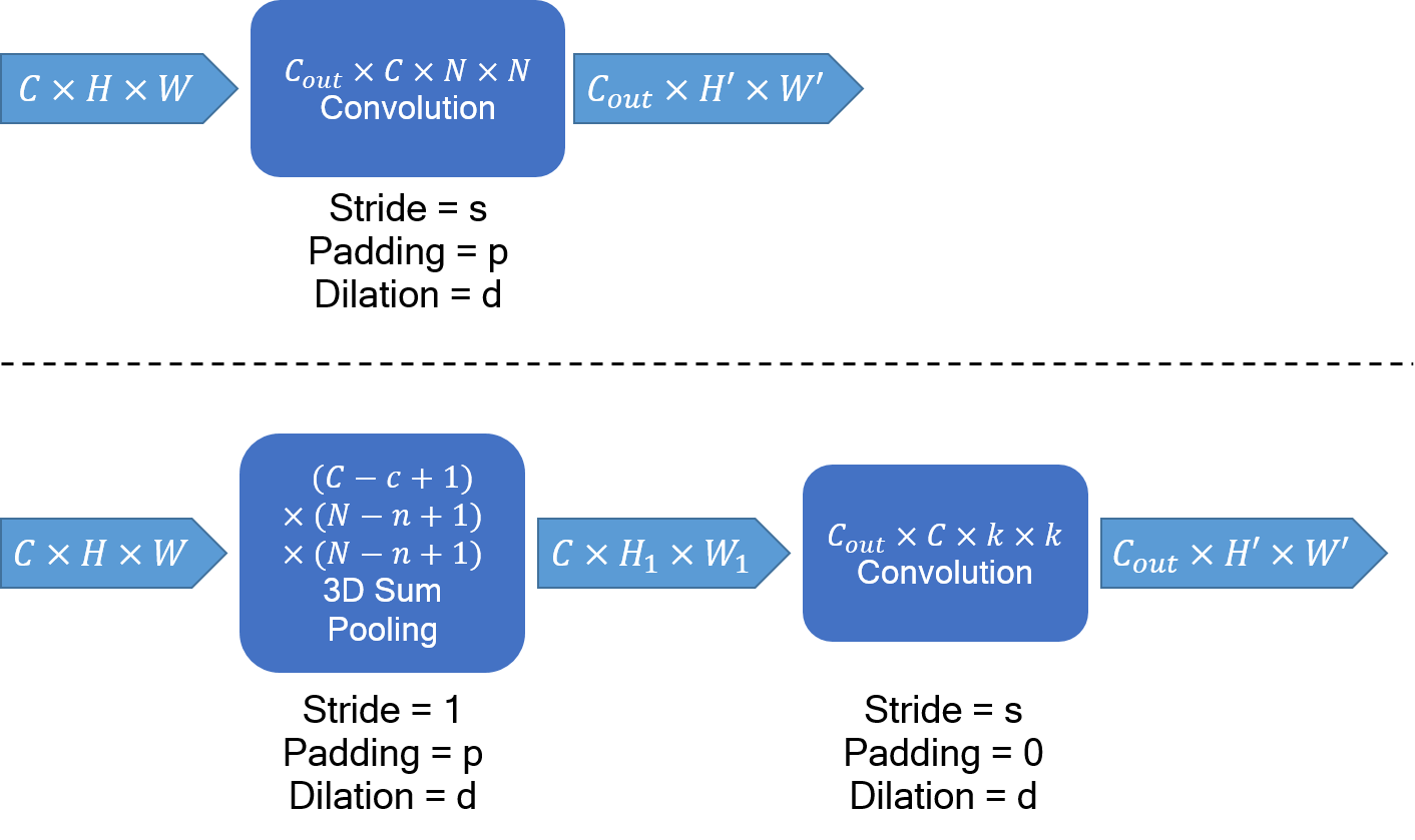
A major advantage of defining Structured Kernels this way is that all the basis elements are just shifted versions of each other (see Fig. 2 and Fig. 1(b)). This means, in Eq. (1), if we consider the convolution $X*W$ for the entire feature map $X$, the summed outputs $X*\beta_{m}$ for all $\beta_{m}$’s are actually the same (except on the edges of $X$). As a result, the outputs $\{X*\beta_{1},...,X*\beta_{cn^{2}}\}$ can be computed using a single sum-pooling operation on $X$ with a kernel size of $(C-c+1)\times(N-n+1)\times(N-n+1)$. Fig. 3 shows a simple example of how a convolution with a $3\!\times\!3$ structured kernel can be broken into a $2\!\times\!2$ sum-pooling followed by a $2\!\times\!2$ convolution with a kernel made of $\alpha_{i}$’s.

Furthermore, consider a convolutional layer of size $C_{out}\!\times\!C\!\times\!N\!\times\!N$ that has $C_{out}$ kernels of size $C{\mkern-1.0mu\times\mkern-1.0mu}N{\mkern-1.0mu\times\mkern-1.0mu}N$. In our design, the same underlying basis $\mathcal{B}=\{\beta_{1},...,\beta_{cn^{2}}\}$ is used for the construction of all $C_{out}$ kernels in the layer. Suppose any two structured kernels in this layer with coefficients $\boldsymbol{\alpha}^{(1)}$ and $\boldsymbol{\alpha}^{(2)}$, i.e. $W_{1}=\sum_{m}\alpha_{m}^{(1)}\beta_{m}$ and $W_{2}=\sum_{m}\alpha_{m}^{(2)}\beta_{m}$. The convolution output with these two kernels is respectively, $X*W_{1}=\sum_{m}\alpha_{m}^{(1)}(X*\beta_{m})$ and $X*W_{2}=\sum_{m}\alpha_{m}^{(2)}(X*\beta_{m})$. We can see that the computation $X*\beta_{m}$ is common to all the kernels of this layer. Hence, the sum-pooling operation only needs to be computed once and then reused across all the $C_{out}$ kernels.

A Structured Convolution can thus be decomposed into a sum-pooling operation and a smaller convolution operation with a kernel composed of $\alpha_{i}$’s. Fig. 4 shows the decomposition of a general structured convolution layer of size $C_{out}\!\times\!C\!\times\!N\!\times\!N$.

Notably, standard convolution ($C{\mkern-1.0mu\times\mkern-1.0mu}N{\mkern-1.0mu\times\mkern-1.0mu}N$), depthwise convolution ($1{\mkern-1.0mu\times\mkern-1.0mu}N{\mkern-1.0mu\times\mkern-1.0mu}N$), and pointwise convolution ($C{\mkern-1.0mu\times\mkern-1.0mu}1{\mkern-1.0mu\times\mkern-1.0mu}1$) kernels can all be constructed as 3D structured kernels, which means that this decomposition can be widely applied to existing architectures. See supplementary material for more details on applying the decomposition to convolutions with arbitrary stride, padding, dilation.

The sum-pooling component after decomposition requires no parameters. Thus, the total number of parameters in a convolution layer get reduced from $C_{out}CN^{2}$ (before decomposition) to $C_{out}cn^{2}$ (after decomposition). The sum-pooling component is also free of multiplications. Hence, only the smaller $c{\mkern-1.0mu\times\mkern-1.0mu}n{\mkern-1.0mu\times\mkern-1.0mu}n$ convolution contributes to multiplications after decomposition.

Before decomposition, computing every output element in feature map $Y\in\mathcal{R}^{C_{out}{\mkern-1.0mu\times\mkern-1.0mu}H^{\prime}{\mkern-1.0mu\times\mkern-1.0mu}W^{\prime}}$ involves $CN^{2}$ multiplications and $CN^{2}-1$ additions. Hence, total multiplications involved are $CN^{2}C_{out}H^{\prime}W^{\prime}$ and total additions involved are $(CN^{2}-1)C_{out}H^{\prime}W^{\prime}$.

After decomposition, computing every output element in feature map $Y$ involves $cn^{2}$ multiplications and $cn^{2}-1$ additions. Hence, total multiplications and additions involved in computing $Y$ are $cn^{2}C_{out}H^{\prime}W^{\prime}$ and $(cn^{2}-1)C_{out}H^{\prime}W^{\prime}$ respectively. Now, computing every element of the intermediate sum-pooled output $E\in\mathcal{R}^{c{\mkern-1.0mu\times\mkern-1.0mu}H_{1}{\mkern-1.0mu\times\mkern-1.0mu}W_{1}}$ involves $((C-c+1)(N-n+1)^{2}-1)$ additions. Hence, the overall total additions involved can be written as:

We can see that the number of parameters and number of multiplications have both reduced by a factor of $\mathbf{{cn^{2}}/{CN^{2}}}$. And in the expression above, if $C_{out}$ is large enough, the first term inside the parentheses gets amortized and the number of additions $\approx(cn^{2}-1)C_{out}H^{\prime}W^{\prime}$. As a result, the number of additions also reduce by approximately the same proportion $\approx cn^{2}/CN^{2}$. We will refer to $CN^{2}/cn^{2}$ as the compression ratio from now on.

Due to amortization, the additions per output are $\approx cn^{2}-1$, which is basically $M-1$ since $M=cn^{2}$.

For image classification networks, the last fully connected layer (sometimes called linear layer) dominates w.r.t. the number of parameters, especially if the number of classes is high. The structural decomposition can be easily extended to the linear layers by noting that a matrix multiplication is the same as performing a number of $1{\mkern-1.0mu\times\mkern-1.0mu}1$ convolutions on the input. Consider a kernel $W\in\mathcal{R}^{P\times Q}$ and input vector $X\in\mathcal{R}^{Q\times 1}$. The linear operation $WX$ is mathematically equivalent to the $1\times 1$ convolution $unsqueezed(X)*unsqueezed(W)$, where $unsqueezed(X)$ is the same as $X$ but with dimensions $Q\times 1\times 1$ and $unsqueezed(W)$ is the same as $W$ but with dimensions $P\times Q\times 1\times 1$. In other words, each row of $W$ can be considered a $1\times 1$ convolution kernel of size $Q\times 1\times 1$.

Now, if each of these kernels (of size $Q\times 1\times 1$) is structured with underlying parameter $R$ (where $R\leq Q$), then the matrix multiplication operation can be structurally decomposed as shown in Fig. 5.

Same as before, we get a reduction in both the number of parameters and the number of multiplications by a factor of $\mathbf{R/Q}$, as well as the number of additions by a factor of $\frac{R(Q-R)+(PR-1)P}{(PQ-1)P}$.

Now, for a structured kernel $W$ characterized by $\{C,N,c,n\}$, there exists a $cn^{2}$ length $\boldsymbol{\alpha}$ such that $W=A\boldsymbol{\alpha}$. Hence, a structured kernel $W$ satisfies the property: $W=AA^{+}W$, where $A^{+}$ is the Moore-Penrose inverse [2] of $A$. Based on this, we propose training a deep network with a Structural Regularization loss that can gradually push the deep network’s kernels to be structured via training:

where $\left\lVert\cdot\right\rVert_{F}$ denotes Frobenius norm and $l$ is the layer index. To ensure that regularization is applied uniformly to all layers, we use $\left\lVert W\right\rVert_{F}$ normalization in the denominator. It also stabilizes the performance of the decomposition w.r.t $\lambda$. The overall proposed training recipe is as follows:

Proposed Training Scheme:

• •

  Step 1: Train the original architecture with the Structural Regularization loss.

  • –

    After Step 1, all weight tensors in the deep network will be almost structured.

• •

  Step 2: Apply the decomposition on every layer and compute $\alpha_{l}=A_{l}^{+}W_{l}$.

  • –

    This results in a smaller and more efficient decomposed architecture with $\alpha_{l}$’s as the weights. Note that, every convolution / linear layer from the original architecture is now replaced with a sum-pooling layer and a smaller convolution / linear layer.

The proposed scheme trains the architecture with the original $C{\mkern-1.0mu\times\mkern-1.0mu}N{\mkern-1.0mu\times\mkern-1.0mu}N$ kernels in place but with a structural regularization loss. The structural regularization loss imposes a restrictive $cn^{2}$ degrees of freedom while training but in a soft or gradual manner (depending on $\lambda$):

1. 1.

   If $\lambda=0$, it is the same as normal training with no structure imposed.

2. 2.

   If $\lambda$ is very high, the regularization loss will be heavily minimized in early training iterations. Thus, the weights will be optimized in a restricted $cn^{2}$ dimensional subspace of $\mathcal{R}^{C{\mkern-1.0mu\times\mkern-1.0mu}N{\mkern-1.0mu\times\mkern-1.0mu}N}$.

3. 3.

   Choosing a moderate $\lambda$ gives the best tradeoff between structure and model performance.

We talk about training implementation details for reproduction, such as hyperparameters and training schedules, in Supplementary material, where we also show our method is robust to the choice of $\lambda$.

We present results for ResNets [10] in Tables 4 and 4. To demonstrate the efficacy of our method on modern networks, we also show results on MobileNetV2 [31] and EfficientNet¹¹1Our Efficientnet reproduction of baselines (B0 and B1) give results slightly inferior to [37]. Our Struct-EffNet is created on top of this EfficientNet-B1 baseline. [37] in Table 4 and 4.

To provide a comprehensive analysis, for each baseline architecture, we present structured counterparts, with version "A" designed to deliver similar accuracies and version "B" for extreme compression ratios. Using different $\{c,n\}$ configurations per-layer, we obtain structured versions with varying levels of reduction in model size and multiplications/additions (please see Supplementary material for details). For the "A" versions of ResNet, we set the compression ratio ($CN^{2}/cn^{2}$) to be 2$\times$ for all layers. For the "B" versions of ResNets, we use nonuniform compression ratios per layer. Specifically, we compress stages 3 and 4 drastically (4$\times$) and stages 1 and 2 by $2\times$. Since MobileNet is already a compact model, we design its "A" version to be $1.33\times$ smaller and "B" version to be $2\times$ smaller.

We note that, on low-level hardware, additions are much power-efficient and faster than multiplications [3, 13]. Since the actual inference time depends on how software optimizations and scheduling are implemented, for most objective conclusions, we provide the number of additions / multiplications and model sizes. Considering observations for sum-pooling on dedicated hardware units [44], our structured convolutions can be easily adapted for memory and compute limited devices.

Compared to the baseline models, the Struct-A versions of ResNets are $2\times$ smaller, while maintaining less than $0.65\%$ loss in accuracy. The more aggressive Struct-B ResNets achieve $60$-$70\%$ model size reduction with about $2$-$3\%$ accuracy drop. Compared to other methods, Struct-56-A is $0.75\%$ better than AMC-Res56 [11] of similar complexity and Struct-20-A exceeds ShiftResNet20-6 [42] by $0.45\%$ while being significantly smaller. Similar trends are observed with Struct-Res18 and Struct-Res50 on ImageNet. Struct-56-A and Struct-50-A achieve competitive performance as compared to the recent GhostNets [7]. For MobileNetV2 which is already designed to be efficient, Struct-MV2-A achieves further reduction in multiplications and model size with SOTA performance compared to other methods, see Table 4. Applying structured convolutions to EfficientNet-B1 results in Struct-EffNet that has comparable performance to EfficientNet-B0, as can be seen in Table 4.

The ResNet Struct-A versions have similar number of adds and multiplies (except ResNet50) because, as noted in Sec. 4.2, the sum-pooling contribution is amortized. But sum-pooling starts dominating as the compression gets more aggressive, as can be seen in the number of adds for Struct-B versions. Notably, both "A" and "B" versions of MobileNetV2 observe a dominance of the sum-pooling component. This is because the number of output channels are not enough to amortize the sum-pooling component resulting from the decomposition of the pointwise ($1\!\times\!1$ conv) layers.

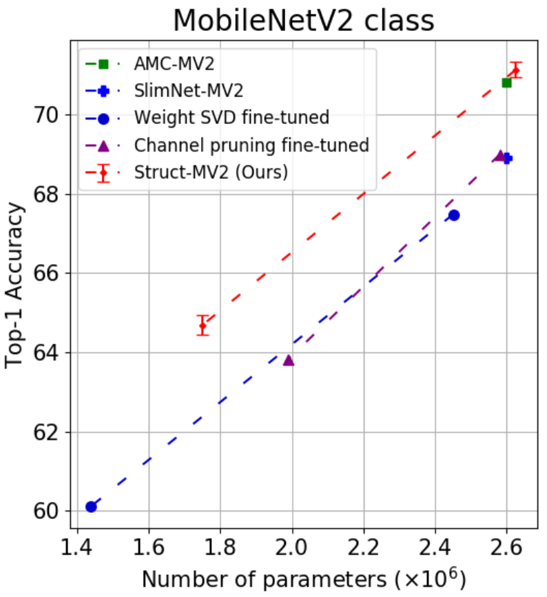
Fig. 6 compares our method with state-of-the-art structured compression methods - WeightSVD [48], Channel Pruning [12], and Tensor-train [35]. Note, the results were obtained from [19]. Our proposed method achieves approximately $1\%$ improvement over the second best method for ResNet18 ($2\times$) and MobileNetV2 ($1.3\times$). Especially for MobileNetV2, this improvement is valuable since it significantly outperforms all the other methods (see Struct-V2-A in Table 4).

After demonstrating the superiority of our method on image classification, we evaluate it for semantic segmentation that requires reproducing fine details around object boundaries. We apply our method to a recently developed state-of-the-art HRNet [39]. Table 5 shows that the structured convolutions can significantly improve our segmentation model efficiency: HRNet model is reduced by 50% in size, and 30% in number of additions and multiplications, while having only 1.5% drop in mIoU. More results for semantic segmentation can be found in the supplementary material.

The proposed method involves computing the Structural Regularization term (3) during training. Although the focus of this work is more on inference efficiency, we measure the memory and time-per-iteration for training with and w/o the Structural Regularization loss on an NVIDIA V100 GPU. We report these numbers for Struct-18-A and Struct-MV2-A architectures below. As observed, the additional computational cost of the regularization term is negligible for a batchsize of $256$. This is because, mathematically, the regularization term, $\sum_{l=1}^{L}\frac{\left\lVert(I-A_{l}A_{l}^{+})W_{l}\right\rVert_{F}}{\left\lVert W_{l}\right\rVert_{F}}$, is independent of the input size. Hence, when using a large batchsize for training, the regluarization term’s memory and runtime overhead is relatively small (less than $5\%$ for Struct-MV2-A and $10\%$ for Struct-18-A).

In our proposed method, we train the architecture with original $C\!\times\!N\!\times\!N$ kernels in place and the regularization loss imposes desired structure on these kernels. At the end of training, we decompose the $C\!\times\!N\!\times\!N$ kernels and replace each with a sum-pooling layer and smaller layer of $c\!\times\!n\!\times\!n$ kernels.

A more direct approach could be to train the decomposed architecture (with the sum-pooling + $c\!\times\!n\!\times\!n$ layers in place) directly. The regularization term is not required in this direct approach, as there is no decomposition step, hence eliminating the computation overhead shown in Table 6. We experimented with this direct training method and observed that the regularization based approach always outperformed the direct approach (by $1.5$% for Struct-18-A and by $0.9$% for Struct-MV2-A). This is because, as pointed out in Sec. 5.1, the direct method optimizes the weights in a restricted subspace of $c\!\times\!n\!\times\!n$ kernels right from the start, whereas the regularization based approach gradually moves the weights from the larger ($C\!\times\!N\!\times\!N$) subspace to the restricted subspace with gradual imposition of the structure constraints via the regularization loss.

References

- [1] Kambiz Azarian, Yash Bhalgat, Jinwon Lee, and Tijmen Blankevoort. Learned threshold pruning. arXiv preprint arXiv:2003.00075, 2020.
- [2] Adi Ben-Israel and Thomas NE Greville. Generalized inverses: theory and applications, volume 15. Springer Science & Business Media, 2003.
- [3] Hanting Chen, Yunhe Wang, Chunjing Xu, Boxin Shi, Chao Xu, Qi Tian, and Chang Xu. Addernet: Do we really need multiplications in deep learning? arXiv preprint arXiv:1912.13200, 2019.
- [4] Marius Cordts, Mohamed Omran, Sebastian Ramos, Timo Rehfeld, Markus Enzweiler, Rodrigo Benenson, Uwe Franke, Stefan Roth, and Bernt Schiele. The cityscapes dataset for semantic urban scene understanding. In Proc. of the IEEE Conference on Computer Vision and Pattern Recognition (CVPR), 2016.
- [5] Emily L. Denton, Wojciech Zaremba, Joan Bruna, Yann LeCun, and Rob Fergus. Exploiting linear structure within convolutional networks for efficient evaluation. In Advances in Neural Information Processing Systems 27: Annual Conference on Neural Information Processing Systems 2014, December 8-13 2014, Montreal, Quebec, Canada, pages 1269–1277, 2014.
- [6] Erich Elsen, Marat Dukhan, Trevor Gale, and Karen Simonyan. Fast sparse convnets. arXiv preprint arXiv:1911.09723, 2019.
- [7] Kai Han, Yunhe Wang, Qi Tian, Jianyuan Guo, Chunjing Xu, and Chang Xu. Ghostnet: More features from cheap operations. arXiv preprint arXiv:1911.11907, 2019.
- [8] Song Han, Huizi Mao, and William J Dally. Deep compression: Compressing deep neural networks with pruning, trained quantization and huffman coding. arXiv preprint arXiv:1510.00149, 2015.
- [9] Song Han, Jeff Pool, John Tran, and William J. Dally. Learning both weights and connections for efficient neural networks. CoRR, abs/1506.02626, 2015.
- [10] Kaiming He, Xiangyu Zhang, Shaoqing Ren, and Jian Sun. Deep residual learning for image recognition. In 2016 IEEE Conference on Computer Vision and Pattern Recognition, CVPR 2016, Las Vegas, NV, USA, June 27-30, 2016, pages 770–778. IEEE Computer Society, 2016.
- [11] Yihui He, Ji Lin, Zhijian Liu, Hanrui Wang, Li-Jia Li, and Song Han. AMC: automl for model compression and acceleration on mobile devices. In Computer Vision - ECCV 2018 - 15th European Conference, Munich, Germany, September 8-14, 2018, Proceedings, Part VII, volume 11211 of Lecture Notes in Computer Science, pages 815–832. Springer, 2018.
- [12] Yihui He, Xiangyu Zhang, and Jian Sun. Channel pruning for accelerating very deep neural networks. In IEEE International Conference on Computer Vision, ICCV 2017, Venice, Italy, October 22-29, 2017, pages 1398–1406, 2017.
- [13] Mark Horowitz. 1.1 computing’s energy problem (and what we can do about it). In 2014 IEEE International Solid-State Circuits Conference Digest of Technical Papers (ISSCC), pages 10–14. IEEE, 2014.
- [14] Max Jaderberg, Andrea Vedaldi, and Andrew Zisserman. Speeding up convolutional neural networks with low rank expansions. arXiv preprint arXiv:1405.3866, 2014.
- [15] Tamara G Kolda and Brett W Bader. Tensor decompositions and applications. SIAM review, 51(3):455–500, 2009.
- [16] Alex Krizhevsky, Geoffrey Hinton, et al. Learning multiple layers of features from tiny images. 2009.
- [17] Anders Krogh and John A Hertz. A simple weight decay can improve generalization. In Advances in neural information processing systems, pages 950–957, 1992.
- [18] Aditya Kusupati, Vivek Ramanujan, Raghav Somani, Mitchell Wortsman, Prateek Jain, Sham Kakade, and Ali Farhadi. Soft threshold weight reparameterization for learnable sparsity. arXiv preprint arXiv:2002.03231, 2020.
- [19] Andrey Kuzmin, Markus Nagel, Saurabh Pitre, Sandeep Pendyam, Tijmen Blankevoort, and Max Welling. Taxonomy and evaluation of structured compression of convolutional neural networks. arXiv preprint arXiv:1912.09802, 2019.
- [20] Vadim Lebedev, Yaroslav Ganin, Maksim Rakhuba, Ivan Oseledets, and Victor Lempitsky. Speeding-up convolutional neural networks using fine-tuned cp-decomposition. arXiv preprint arXiv:1412.6553, 2014.
- [21] Vadim Lebedev and Victor Lempitsky. Fast convnets using group-wise brain damage. In Proceedings of the IEEE Conference on Computer Vision and Pattern Recognition, pages 2554–2564, 2016.
- [22] Fengfu Li and Bin Liu. Ternary weight networks. arXiv preprint arxiv:1605.04711, 2016.
- [23] Hao Li, Asim Kadav, Igor Durdanovic, Hanan Samet, and Hans Peter Graf. Pruning filters for efficient convnets. In 5th International Conference on Learning Representations, ICLR 2017, Toulon, France, April 24-26, 2017, Conference Track Proceedings. OpenReview.net, 2017.
- [24] Ji Lin, Chuang Gan, and Song Han. Tsm: Temporal shift module for efficient video understanding. In Proceedings of the IEEE International Conference on Computer Vision, pages 7083–7093, 2019.
- [25] Zhuang Liu, Mingjie Sun, Tinghui Zhou, Gao Huang, and Trevor Darrell. Rethinking the value of network pruning. arXiv preprint arXiv:1810.05270, 2018.
- [26] Stéphane Mallat. Group invariant scattering. Communications on Pure and Applied Mathematics, 65(10):1331–1398, 2012.
- [27] Franco Manessi, Alessandro Rozza, Simone Bianco, Paolo Napoletano, and Raimondo Schettini. Automated pruning for deep neural network compression. In 24th International Conference on Pattern Recognition, ICPR 2018, Beijing, China, August 20-24, 2018, pages 657–664. IEEE Computer Society, 2018.
- [28] Ivan V Oseledets. Tensor-train decomposition. SIAM Journal on Scientific Computing, 33(5):2295–2317, 2011.
- [29] Qiang Qiu, Xiuyuan Cheng, Robert Calderbank, and Guillermo Sapiro. Dcfnet: Deep neural network with decomposed convolutional filters. arXiv preprint arXiv:1802.04145, 2018.
- [30] Olga Russakovsky, Jia Deng, Hao Su, Jonathan Krause, Sanjeev Satheesh, Sean Ma, Zhiheng Huang, Andrej Karpathy, Aditya Khosla, Michael Bernstein, Alexander C. Berg, and Li Fei-Fei. ImageNet Large Scale Visual Recognition Challenge. International Journal of Computer Vision (IJCV), 115(3):211–252, 2015.
- [31] Mark Sandler, Andrew Howard, Menglong Zhu, Andrey Zhmoginov, and Liang-Chieh Chen. Mobilenetv2: Inverted residuals and linear bottlenecks. In The IEEE Conference on Computer Vision and Pattern Recognition (CVPR), June 2018.
- [32] Laurent Sifre and Stéphane Mallat. Rotation, scaling and deformation invariant scattering for texture discrimination. In Proceedings of the IEEE conference on computer vision and pattern recognition, pages 1233–1240, 2013.
- [33] Nitish Srivastava, Geoffrey Hinton, Alex Krizhevsky, Ilya Sutskever, and Ruslan Salakhutdinov. Dropout: a simple way to prevent neural networks from overfitting. The journal of machine learning research, 15(1):1929–1958, 2014.
- [34] Gilbert Strang. A proposal for toeplitz matrix calculations. Studies in Applied Mathematics, 74(2):171–176, 1986.
- [35] Jiahao Su, Jingling Li, Bobby Bhattacharjee, and Furong Huang. Tensorized spectrum preserving compression for neural networks. arXiv preprint arXiv:1805.10352, 2018.
- [36] Cheng Tai, Tong Xiao, Yi Zhang, Xiaogang Wang, et al. Convolutional neural networks with low-rank regularization. arXiv preprint arXiv:1511.06067, 2015.
- [37] Mingxing Tan and Quoc V Le. Efficientnet: Rethinking model scaling for convolutional neural networks. arXiv preprint arXiv:1905.11946, 2019.
- [38] Muhammad Tayyab and Abhijit Mahalanobis. Basisconv: A method for compressed representation and learning in cnns. arXiv preprint arXiv:1906.04509, 2019.
- [39] Jingdong Wang, Ke Sun, Tianheng Cheng, Borui Jiang, Chaorui Deng, Yang Zhao, Dong Liu, Yadong Mu, Mingkui Tan, Xinggang Wang, Wenyu Liu, and Bin Xiao. Deep high-resolution representation learning for visual recognition. TPAMI, 2019.
- [40] Yunhe Wang, Chang Xu, XU Chunjing, Chao Xu, and Dacheng Tao. Learning versatile filters for efficient convolutional neural networks. In Advances in Neural Information Processing Systems, pages 1608–1618, 2018.
- [41] Wei Wen, Chunpeng Wu, Yandan Wang, Yiran Chen, and Hai Li. Learning structured sparsity in deep neural networks. In Advances in neural information processing systems, pages 2074–2082, 2016.
- [42] Bichen Wu, Alvin Wan, Xiangyu Yue, Peter Jin, Sicheng Zhao, Noah Golmant, Amir Gholaminejad, Joseph Gonzalez, and Kurt Keutzer. Shift: A zero flop, zero parameter alternative to spatial convolutions. In Proceedings of the IEEE Conference on Computer Vision and Pattern Recognition, pages 9127–9135, 2018.
- [43] Yinchong Yang, Denis Krompass, and Volker Tresp. Tensor-train recurrent neural networks for video classification. In Proceedings of the 34th International Conference on Machine Learning-Volume 70, pages 3891–3900. JMLR. org, 2017.
- [44] Reginald Clifford Young and William John Gulland. Performing average pooling in hardware, July 24 2018. US Patent 10,032,110.
- [45] Jiahui Yu, Linjie Yang, Ning Xu, Jianchao Yang, and Thomas Huang. Slimmable neural networks. arXiv preprint arXiv:1812.08928, 2018.
- [46] Tianyun Zhang, Shaokai Ye, Kaiqi Zhang, Jian Tang, Wujie Wen, Makan Fardad, and Yanzhi Wang. A systematic DNN weight pruning framework using alternating direction method of multipliers. In Computer Vision - ECCV 2018 - 15th European Conference, Munich, Germany, September 8-14, 2018, Proceedings, Part VIII, volume 11212 of Lecture Notes in Computer Science, pages 191–207. Springer, 2018.
- [47] Xiangyu Zhang, Jianhua Zou, Kaiming He, and Jian Sun. Accelerating very deep convolutional networks for classification and detection. IEEE Trans. Pattern Anal. Mach. Intell., 38(10):1943–1955, 2016.
- [48] Xiangyu Zhang, Jianhua Zou, Kaiming He, and Jian Sun. Accelerating very deep convolutional networks for classification and detection. IEEE transactions on pattern analysis and machine intelligence, 38(10):1943–1955, 2016.
- [49] Hengshuang Zhao, Jianping Shi, Xiaojuan Qi, Xiaogang Wang, and Jiaya Jia. Pyramid scene parsing network. In Proceedings of the IEEE conference on computer vision and pattern recognition, pages 2881–2890, 2017.
- [50] Huasong Zhong, Xianggen Liu, Yihui He, and Yuchun Ma. Shift-based primitives for efficient convolutional neural networks. arXiv preprint arXiv:1809.08458, 2018.
Appendix A Appendix
A.1 Structured Convolutions with arbitrary Padding, Stride and Dilation
In the main paper, we showed that a Structured Convolution can be decomposed into a Sum-Pooling component followed by a smaller convolution operation with a kernel composed of the ’s. In this section, we discuss how to calculate the equivalent stride, padding and dilation needed for the resulting decomposed sum-pooling and convolution operations.
A.1.1 Padding
The easiest of these three attributes is padding. Fig. 7 shows an example of a structured convolution with a kernel (i.e. ) with underlying parameter . Hence, it can be decomposed into a sum-pooling operation followed by a convolution. As shown in the figure, to preserve the same output after the decomposition, the sum-pooling component should use the same padding as the original convolution, whereas the smaller convolution is performed without padding.
This leads us to a more general result that - if the original convolution uses a padding of , then, after the decomposition, the sum-pooling should be performed with padding and the smaller convolution (with ’s) should be performed without padding.
A.1.2 Stride
The above rule can be simply extended to the case where the original structured convolution has a stride associated with it. The general rule is - if the original convolution uses a stride of , then, after the decomposition, the sum-pooling should be performed with a stride of and the smaller convolution (with ’s) should be performed with a stride of .
A.1.3 Dilation
Dilated or atrous convolutions are prominent in semantic segmentation architectures. Hence, it is important to consider how we can decompose dilated structured convolutions. Fig. 8 shows an example of a structured convolution with a dilation of . As can be seen in the figure, to preserve the same output after decomposition, both the sum-pooling component and the smaller convolution (with ’s) has to be performed with a dilation factor same as the original convolution.
Fig. 9 summarizes the aforementioned rules regarding padding, stride and dilation.
A.2 Training Implementation Details
Image Classification. For both ImageNet and CIFAR-10 benchmarks, we train all the ResNet architectures from scratch with the Structural Regularization (SR) loss. We set to for the Struct-A versions and for the Struct-B versions throughout training. For MobileNetV2, we first train the deep network from scratch without SR loss (i.e. ) for epochs to obtain pretrained weights and then apply SR loss with for further epochs. For EfficientNet-B0, we first train without SR loss for epochs and then apply SR loss with for further epochs.
For CIFAR-10, we train the ResNets for epochs using a batch size of and an initial learing rate of which is decayed by a factor of at and epochs. We use a weight decay of throughout training. On ImageNet, we use a cosine learning rate schedule with an SGD optimizer for training all architectures. We train the ResNets using a batch size of and weight decay of for epochs starting with an initial learning rate of .
For MobileNetV2, we use a weight decay of and batch size throughout training. In the first phase (with ), we use an initial learning rate of for epochs and in the second phase, we start a new cosine schedule with an initial learning rate of for the next epochs. We train EfficientNet-B0 using Autoaugment, a weight decay of and batch size . We use an initial learning rate of in the first phase and we start a new cosine schedule for the second phase with an initial learning rate of for the next epochs.
Semantic Segmentation. For training Struct-HRNet-A on Cityscapes, we start from a pre-trained HRNet model and train using structural regularization loss. We set to . We use a cosine learning rate schedule with an initial learning rate of . The use image resolution of for training, same as the original image size. We train for 90000 iterations using a batch size of 4.
A.3 Additional results on Semantic Segmentation
In Table 8 and 8, we present additional results for HRNetV2-W18-Small-v1 [39] (note this is different from HRNetV2-W18-Small-v2 reported in the main paper) and PSPNet101 [49] on Cityscapes dataset.