Structure-Preserving Model Reduction for Nonlinear Power Grid Network
††thanks: This work was supported in parts by National Science Foundation under
Grant No. DMS-1923221
Abstract
We develop a structure-preserving system-theoretic model reduction framework for nonlinear power grid networks. First, via a lifting transformation, we convert the original nonlinear system with trigonometric nonlinearities to an equivalent quadratic nonlinear model. This equivalent representation allows us to employ the -based model reduction approach, Quadratic Iterative Rational Krylov Algorithm (Q-IRKA), as an intermediate model reduction step. Exploiting the structure of the underlying power network model, we show that the model reduction bases resulting from Q-IRKA have a special subspace structure, which allows us to effectively construct the final model reduction basis. This final basis is applied on the original nonlinear structure to yield a reduced model that preserves the physically meaningful (second-order) structure of the original model. The effectiveness of our proposed framework is illustrated via two numerical examples.
Index Terms:
Power network grids, lifting, nonlinear model reduction, structured model reduction, -norm.I Introduction
Power networks are complex and large-scale systems in operation. Simulation of these high dimensional power system models are computationally expensive and demand unmanageable levels of storage in dynamic simulation or trajectory sensitivity analysis. Hence, reducing the order of these models is of a great importance especially for real time applications, stability analysis, and control design [12].
Numerous model order reduction (MOR) techniques have been applied to the linearized power networks models including balanced truncation [20, 11, 32, 36, 18], Krylov subspace (interpolatory) methods [8, 38, 39, 35], proper orthogonal decomposition (POD) [41], singular perturbation theory [27, 13], sparse representation of the system matrices [19], and clustering analysis [10, 37, 16, 23]. For a comparative study of MOR techniques in power systems, see, e.g., [7, 1, 12]. Recently, development of MOR techniques for nonlinear systems including power networks has received great attention. In [28], POD is employed to reduce the hybrid, nonlinear model of a power network for the study of cascading failures. Trajectory piece-wise linearization (TPWL) method to approximate the nonlinear term in swing models together with POD to find a reduced order model for the swing dynamics was employed in [21]. Balanced truncation based on empirical controllability and observability covariances of nonlinear power systems is proposed in [30]. The empirical Gramians and balanced realization were also used in [42, 43] to build a nonlinear power system model suitable for controller design. In [29], real-time phasor measurements are used to cluster generators based on similar behaviors using recursive spectral bipartitioning and spectral clustering. The reduced model is formed by representative generators chosen from each cluster. A model reduction approach that adaptively switches between a hybrid system with selective linearization and a linear system based on the variations of the system state or size of a disturbance was developed in [26]. A structure-preserving, aggregation-based model order reduction framework based on synchronization properties of power systems is introduced in [24]. In [40] an SVD-based approach for real-time dynamic model reduction with the ability of preserving some nonlinearity in the reduced model is presented. The recent work [33] presents the idea of transforming the swing equations into a quadratic system, lifts nonlinear swing equations to a quadratic one, and employs quadratic balanced truncation model order reduction technique. A non-intrusive data-driven modeling framework for power network dynamics using Lift and Learn [31] has been studied in [34].
In this paper, we focus on designing a structure-preserving and input-independent MOR framework for a special class of power grid networks. We obtain the reduction bases using the idea of lifting the nonlinear dynamics to quadratic models and employing -quasi-optimal model reduction for quadratic systems (Q-IRKA) [6]. The reduction basis for the second-order nonlinear power network grids model is obtained with the help of the reduction bases obtained by Q-IRKA and their particular subspace structure. This reduction basis is then applied on the second-order nonlinear power network grids model to form a structure-preserving reduced model.
The rest of the paper is organized as follows: Section II briefly introduces the nonlinear dynamical model of the power grid network followed by a quick recap of projection-based structure-preserving model reduction in this setting in Section III. Section IV illustrates how to lift the second-order dynamics of the power grid network to quadratic dynamics and presents an equilibrium analysis. In Section V, we describe the model reduction for quadratic systems via the -based model reduction, Q-IRKA, followed by the required modification for the quadratized power grid model before employing -based model reduction. In Section VI, we present our structured-preserving model reduction approach for power grid networks by proving and exploiting the specific structure arising in Q-IRKA for these dynamics. Section VII illustrates the feasibility of our approach via numerical examples and by comparing our approach with two other methods, followed by conclusions in Section VIII.
II power grid network model
There are three most commonly used models for describing a dynamical model of a power grid network: synchronous motor (), effective network () and structure-preserving (). Each model is described as a network of coupled oscillators (generators or loads) whose dynamics at the th node is expressed by the nonlinear second-order equation [25]
| (1) |
where is the angle of rotation for the th oscillator; and are inertia and damping constants, respectively; is the angular frequency for the system; is dynamical coupling between oscillator and ; and is the phase shift in this coupling. Constants , and are computed by solving the power flow equations and applying Kron reduction [25]. The three models mainly differ by the way they model loads. The EN model assumes loads as constant impedances instead of oscillators. The SP model represents loads as first-order oscillators () while the SM model represent loads as synchronous motors expressed as second-order oscillators.
Define the state-vector . Then, the dynamics of a network of coupled oscillators, given in (1) for the th node, can be described in the system form
| (2) | ||||
| (3) |
where the matrices , , and are defined as
| (6) |
where and , is input to the dynamics; and the nonlinear map is defined such that its th component for is
| (7) |
The variable in (3) corresponds to the output (quantity of interest) of the network dynamics, described by the state-to-output matrix .
III Structure-preserving MOR approach
Large scale power network dynamics, i.e., those with large , are computationally expensive to simulate and control. With the aid of the model reduction, we are able to replace these high dimensional models by lower dimensional models that can closely mimic the input-output behavior of the original high dimensional systems. To be more specific, we seek to develop a nonlinear structure-preserving model reduction approach such that the reduced model preserves the physically-meaningful second-order structure. In other words, we directly reduce the second-order dynamics (2)-(3) to obtain a reduced second-order system with dimension and of the form
| (8) | ||||
| (9) |
where is the reduced state; ; ; ; and . The goal of this structure-preserving model reduction process is that approximates the original output with high fidelity.
Given the full-order dynamics (2)-(3), the most common approach for constructing the reduced model (8)-(9) is the Petrov-Galerkin projection framework: Construct two model reduction bases such that . Insert into (2) and enforce a Petrov-Galerkin condition on the residual to obtain the reduced matrices in (8) and (9) as
| (12) |
To preserve the symmetry and positive definiteness of and in (8), we employ a Galerkin projection by setting . However, unlike the usual MOR via Galerkin projection where the subspace (and thus ) only contains information from the dynamics equation (2) and ignores the output equation (3), our one-sided Galerkin projection will contain information from both (2) and (3) by taking advantage of the special structure arising in the network dynamics. These issues are discussed in detail in Section VI. The term in (12) is usually further approximated to resolve the lifting bottleneck [9]. Due to the page limit, we skip this detail here.
The accuracy of the structure-preserving reduced model (8) depends on the proper choice of . For general nonlinearities, POD is usually the method of choice. However, for special classes of nonlinear systems such as bilinear and quadratic-bilinear systems, one can indeed use well-established system theoretical methods; see, e.g., [6, 5, 3]. A large class of nonlinear systems, such as those with smooth nonlinearities, e.g., exponential, trigonometric, can indeed be represented as quadratic-bilinear systems by introducing new variables (in a lifting map) [22], [14], [4], [33], [31]. Converting a nonlinear model to its equivalent quadratic form provides an opportunity to perform input-independent model reduction techniques where a system-theoretic norm is defined [5, 6]. Although this transformation is not unique, it is exact in many cases (as in here), i.e., there is no approximation error [5].
Second-order model (1) inherently contains a quadratic nonlinearity in and the nonlinear system (2) can be lifted to a quadratic dynamic as we will see next in Section IV. However, as stated in section (III), we seek to obtain a reduced second-order model, not a reduced quadratic model. Therefore, by exploiting the inherent structure of the model reduction bases obtained for the quadratic model, we form the final reduction base to construct the final structure preserving reduced model (12). This is achieved in Sections V–VI.
IV Quadratic representation
As we mentioned in Section III for systems with quadratic nonlinearities, effective and in some cases optimal, systems-theoretic MOR methods already exist. Therefore, in obtaining high-fidelity reduced models, we can significantly benefit from a quadratic representation of the nonlinear swing dynamics.
Towards this goal, recall the original second-order dynamics (1). Expand the nonlinearity using the trigonometric identity and introducing and
| (13) | ||||
Note that equation (13) is quadratic in and . This directly hints at choosing and as auxiliary variables in a new state vector to convert the nonlinear dynamics to a quadratic one. This is precisely what has been done in [33] to find a quadratic representation for (2). However, since the transformation, the so-called lifting, is not unique and we have a slightly different form in the resulting state-space form, we include its derivation here for completeness.
Lemma 1.
Proof.
The proof is constructive, i.e., it will show how the matrices and in (17) will be constructed. Using the new state vector in (1), we can directly rewrite the original output as as in (17) with
| (18) |
It follows from (2) and (1) that
| (19) | ||||
| (20) | ||||
| (21) | ||||
| (22) |
where denotes the Hadamard product.
We start by writing in (21) and in (22) as
| (23) |
where and has zero entries except for the th diagonal element, which is . Next, we write the nonlinearity in (20) as a quadratic term. Towards this goal, we use (13) in (7) to obtain
| (24) | ||||
Using (24), we can write the vector compactly as
| (25) |
where consists of block matrices defined as
| (26) |
Similarly, we have and for the block of , denoted by , we have
| (27) |
Using (23) and (25), we now rewrite (19)-(22) as
| (28) | ||||
| (29) | ||||
| (30) | ||||
| (31) |
Note that the new formulation of the dynamics in (28)-(31) only contains linear and quadratic terms in , and the input mapping is linear. The output mapping is already established in (18). Therefore, there exist matrices and such that the original power network dynamics can be written as a quadratic nonlinear system as in (17), thus proving the desired result. However, to give a constructive proof, we continue to show how the matrices in (17) can be explicitly constructed.
It immediately follows from (28)-(31) that , , and in (17) (corresponding to the linear parts of the dynamics) are given by
| (32) | ||||
| (33) |
where denotes the identity matrix (of appropriate size). To show how is constructed, we define a revised Kronecker product as
| (34) |
where , for . Clearly, (34) is a permuted form of the regular Kronecker product. It is introduced here to make the derivation of easier. The quadratic terms (29)-(31) can be written as
| (35) |
Decompose into four sub-matrices:
| (36) |
where for . The first submatrix corresponds to the first block of (34), i.e, . There is no term in (28)-(31). Thus, we set .
Similarly, the matrix corresponds to the second block of (34), i.e, . We can see from (28)-(31) that two terms, namely and , exist in (30) and (31), respectively. One can rewrite (30) as and allocate the first term, i.e., in , to . More specifically and by using the MATLAB notation for row and column indices, we set the . (The second term in , i.e.,, will be matched by below). Similarly, we can write (31) as and allocate the first term to by setting (the second term will be matched via ). Thus, we set
| (37) |
Following similar arguments, we obtain
| (38) |
Since (34) is a permuted form of , there exists a permutation matrix such that
| (39) |
where . Then, in (17) is
| (40) |
∎
IV-A Equilibrium analysis
So far we have represented the power network dynamics in two formats: as second-order dynamics in (2)-(3) and as quadratic dynamics in (17). In this section, we investigate how the lifting transformation (1) affects the equilibrium points.
To find the equilibrium points of (2), first we transform it to a first-order form by defining a state vector to obtain
| (41) |
using . Let be an equilibrium point of (41). By setting , we obtain that satisfies
| (42) |
Lemma 2.
Proof.
Rewrite (41) as
| (45) |
where . If in (42) is an equilibrium of (45), then we have . Now, let us write (1) as
| (46) |
where is the quadratic lifting in (1), given by
| (47) |
Differentiate (46) to obtain
| (48) |
where the Jacobian is given by
| (49) |
Insert into (48) to obtain proving that (43) is an equilibrium of (17).
V Model reduction for quadratic systems
Now that we have represented the original nonlinear swing dynamics as an equivalent quadratic dynamics, we will investigate the MOR problem for those systems in more details.
Consider the quadratic dynamical system
| (50) |
where , , , and . One can view as the mode-1 matricization of a third-order tensor . In other words, let for be the frontal slices of . Then,
| (51) |
where the notation denotes the mode-1 matricization.
For the cases where the state-space dimension is large, the goal is to find a reduced quadratic system
| (52) |
where , and with such that for a wide range of inputs. We construct the reduce system (52) via projection: Construct two model reduction bases , such that the reduced matrices in (52) are given by
| (53) |
The quality of the reduced system (52) depends on the choice of the model reduction bases and . There are various model reduction techniques to determine theses bases including trajectory-based method such as POD (see, e.g., [15]); and input-independent systems theoretic methods for quadratic systems such as balanced truncation [5], [33], interpolatory projections [4], [14] and -quasi-optimal model reduction [6]. In this paper, we employ the -based approach in [6].
V-A -based model reduction of quadratic nonlinearities
Consider the original quadratic dynamics (50) with an asymptotically stable matrix . Define a truncated norm for (50) denoted by using the three leading Volterra kernels as [6]:
| (54) | ||||
where , ,
and denotes the trace of the argument (for details see, e.g., [6, 2]). Note that when , only the first kernel remains and accordingly (54) boils down to the classical -norm of an asymptotically stable linear system.
The goal is now to construct and such that the truncated error norm is minimized. This can be achieved by the model reduction algorithm Q-IRKA [6]. A brief sketch of (the two-sided) Q-IRKA is shown in Algorithm 1. In some settings, to retain the positive definiteness and/or symmetry of the original realization in the reduced order matrices (V), a one sided version of Q-IRKA is applied where is set to as given in Algorithm 2. The proposed approach to structure preserving model reduction of power networks as outlined in the next section will employ Q-IRKA as an intermediate step. Note that the reduced models from Q-IRKA is quadratic, do not preserve the original second-order structure (2), and thus cannot be directly used in a structure preserving setting. In the next section, we will prove that the model reduction basis and resulting from applying Q-IRKA to the quadratic form of power network have special subspace structure, which will then allow us to develop our structure-preserving model reduction algorithm.
V-B Modifications to perform Q-IRKA for power network dynamics: zero initial conditions and asymptotic stability
Recall the state vector in (1). Since and can not be simultaneously zero, the reformulation (17) as a quadratic model will always have a nonzero initial condition. Since the most system theoretic methods to model reduction assumes a zero initial condition, a natural approach is to consider a shifted state vector that allows the use of the reduction methods developed for zero initial condition. Following [33], we define a shifted state vector , such that in the new state , we have and write
| (55) |
By substituting (55) in (17) we obtain
| (58) |
| (59) |
Given the dynamical system (V-B) with zero initial conditions, one can apply a wide range of available methods, as mentioned at the beginning of Section V, to construct a quadratic reduced model. However, as in the linear case, optimal- model reduction for quadratic system requires asymptotic stability of [6]. Recall the quadratic dynamics (58) and in (V-B). Consider zero initial conditions for and , and thus the initial condition . Thus, have zero eigenvalues and therefore is not asymptotically stable [33]. To overcome this stability issue in the power network setting, we replace in (58) by
| (60) |
where is real and small, so that all the eigenvalues of the pair and have negative real part. Therefore, as the final modification, we replace (58) by
| (63) |
The quadratic dynamical system in (63) has now asymptotically stable linear part and have zero initial conditions. Therefore, it has the structure to perform based model reduction using Q-IRKA. However, we re-emphasize that the reduced-model obtained from applying Q-IRKA to (63) is not structure-preserving; it does not inherit the second-order structure. Therefore, we employ Q-IRKA only to obtain potential reduction subspace information. In the next section where we present the proposed framework, we describe how we benefit from and how we use the subspaces resulting from Q-IRKA to obtain a reduced second-order model in (8). We also show that Q-IRKA subspaces applied to (63) has special properties due to the underlying power network structure.
VI The proposed approach for MOR of Power Networks
Our aim is to perform structure-preserving model reduction of the second-order dynamics (2)-(3) using the reduction bases to obtain the reduced second-order model (8)-(12). To keep the symmetry of the underlying dynamics, we perform a Galerkin projection by choosing . Converting the nonlinear second-order dynamics to the quadratic form has allowed us to use (optimal) systems-theoretic techniques to apply, such as Q-IRKA. Although we cannot simply use the output of Q-IRKA as the reduced model (since it does not preserve the second-order structure), we still would like to employ the high-fidelity model reduction bases and resulting from Q-IRKA in constructing . In this section, by analyzing and exploiting the structure of the underlying power network dynamics, we show how to efficiently construct using and from Q-IRKA.
VI-A Structures arising in Q-IRKA in the Power Network Setting
Let and be the model reduction bases obtained from applying Q-IRKA to (63). Let and denote leading rows of and . Recall that due to (1), the leading rows of , the state of quadratic dynamic (63), corresponds to the original (second-order) state . Therefore, one can consider choosing and in (12). However, in addition to this being a Petrov-Galerkin projection and thus not preserving the symmetry, we will show in the next result has a particular subspace structure that one can further exploit in constructing the structured reduced model.
Theorem 1.
Before we prove Theorem 1, we establish a symmetry property of that will be used in its proof.
Lemma 3.
Let in (63) be the mode-1 matricization of the third order tensor , Then, the tensor is symmetric, i.e., for every , it holds
| (65) |
Proof.
Recall (39) and (40), and rewrite as
where and with Using (34) and (36) we obtain
| (66) |
Let . Multiply (66) from the right with to pick the first rows of . Since the first rows of and are zero as can be seen in (37) and (38), we have Similarly, Therefore, we have
| (67) |
Now let and multiply (66) from the right with :
| (68) |
Let be the permutation matrix so that
| (69) |
where is partitioned as and each , for , is defined as
| (70) |
where denotes the th column of a identity matrix. Insert (69) into (VI-A) to obtain
| (71) | ||||
Then, form ,
| (72) |
where, using (70) we have, for ,
| (73) |
and is the MATLAB notation referring to the th column of . Since for the coupling between the oscillators and , we have and , we can write and accordingly rewrite (73) as
| (74) |
Then, inserting (74) into (72) yields
| (75) |
Similarly, one can show that
| (76) |
Plug (75) and (76) into (71) to obtain
| (77) |
Following similar steps, one obtains
| (78) |
where and . Combining (67), (77), and (78), we conclude (65), i.e., is symmetric. ∎
Now we are ready to prove Theorem 1.
Proof.
(of Theorem 1) We start by analyzing the first Sylvester equation involving in Step 7 of Algorithm 1:
| (79) |
where contains the eigenvalues of , , and
| (80) |
Recall in (40):
| (81) |
Multiply by the first unit vector from the right to obtain
| (82) |
where denotes the first column of . Now, we apply Lemma 3 to (82) and use (81) to obtain
| (83) |
Similarly, for the th column of (81), we obtain
| (84) |
Therefore, (83) and (84) reveal that the first columns of are zero. Using this fact, and (32) and (33), we obtain the first columns of (80) as
| (85) |
where refers to the first columns of the matrix . Decompose where . Recall (18) and (32), and use (85) in (79) to obtain .
Recall that is a positive real number and the reduced order poles are assumed in the left-half plane. Therefore, the matrix is invertible and Similarly, let and solve for the first block of denoted by in the second Sylvester equation in Step 7 of Algorithm 1:
| (86) |
Next, we will prove that the first rows of are zero. Towards this goal, recall (51) and let be partitioned as
| (87) |
where for . From (81), we know that the leading columns are zero. Therefore, we write
| (88) |
i.e., for . Recall that is symmetric due to Lemma 3. This means that
| (89) |
where Since for , we obtain
| (90) |
Due to (89), the first rows of are the first columns of . Then, (90) implies that . Using this fact in (86) yields . Since is invertible, we obtain . Recall in Step of Algorithm (1) defined as . Then, for the first rows of , i.e., for , we obtain
| (91) |
Hence, , which proves (64). In addition, if , the matrix has a right-inverse and thus the reverse direction holds as well, i.e., , completing the proof of the theorem. ∎
We emphasize that the structure of the range of due to Q-IRKA as shown in Lemma 1 is specific to the underlying power network dynamics and its quadratic form. The authors are not aware of any other models that yield such a form. This result will be crucial in forming the proposed algorithm next.
VI-B Proposed structure-preserving model reduction algorithm
Lemma 1 states that whenever (which will be the common situation), is rank-deficient. Therefore, even though this means that is not suitable to be used as a model reduction space as is, we can use it to our advantage.
As noted earlier, we will perform Galerkin projection. In other words, in (12) we will use . One option is to simply ignore and set . However, this is not preferred in an input-output based systems-theoretic model reduction setting since the information in related to the output is fully ignored. Fortunately, due to the subspace result (64) in Theorem 1, we can include both the input-to-state subspace information () and the state-to-output subspace information () in one subspace by choosing in (12) as
| (92) |
where “orth” refers to forming an orthonormal basis so that . Then, we choose and perform a Galerkin projection to compute the reduced second-order structure-preserving model (8)-(12). Thus, despite performing a one-sided Galerkin, by exploiting Theorem 1 and using the reduction basis in (92), we are able to also incorporate the output information in the reduction framework, as is the standard in systems theoretic model reduction. We note that for the column dimension of , we have .
Now, we finally summarize our proposed approach, an -based Structure-preserving MOR method for Power Network Dynamics (StrH2), in Algorithm 3. We start by converting the original dynamics to the equivalent quadratic form in Step 1. Then, in Step 2, we either apply two-sided Q-IRKA (Algorithm 1) or one-sided Q-IRKA (Algorithm 2) to the resulting quadratic-system to construct . The resulting versions of the proposed method will be labeled as StrH2-A and StrH2-B, respectively. Step 3 constructs the final model reduction basis using the analysis of Theorem 1 and Step 4 constructs the final structured reduced-model.
We note that in (92), the -subspace information is not needed since it is already contained in . However, StrH2-A version of Algorithm 3, in Step 2, still uses two-sided Q-IRKA, which computes during the iteration unlike in one-sided Q-IRKA where the -subspace is never computed. One might think that since the -subspace information is replaced by in the end, the two options StrH2-A and StrH2-B should produce equivalent results. This is indeed not the case since the -subspace resulting from one-sided and two-sided Q-IRKA implementations are completely different; the former never used the output information. We will see in next section that this distinction does indeed impact the final reduced model.
VII Numerical Experiments
We test the proposed approach on two models: (i) the SM model of the 39-bus New England test system and (ii) IEEE 118 bus system, included in the MATPOWER software toolbox [44],[45]. We focus on a single-output system by choosing the arithmetic mean of all phase angles as the output as in [34, 33]. Models are generated by MATPOWER and MATLAB toolbox pg-sync-models [25] that provide all the necessary parameters to form (2) including , , , , and . To illustrate the effectiveness of our approach, we compare it with two other approaches (i) a structure-preserving formulation of balanced truncation for power systems denoted by Str-QBT and (ii) POD.
For Str-QBT, we follow the approach of [33] in finding and . However, as opposed to [33], which performs the reduction on the quadratic dynamics (63) and constructs a quadratic reduced model, we directly find the reduced second order dynamic (8) by extracting and from and . To be more precise, [33] forms the reduction bases as
| (96) |
and similarly for using where and are
| (99) |
is the SVD of , and and are, respectively, the Cholesky factors of the second block of the truncated reachability and observability gramians of the quadratic system [5], [33]. Then, [33] performs the reduction on (63) using (96) to obtain a reduced quadratic model for (63). Instead, since the second blocks of the truncated reachability and observability gramians of the quadratic system correspond to the second order dynamic (2), we pick and in (12) and directly perform reduction on the second order dynamic (2)-(3) to obtain (8), (9).
To apply POD, we simulate (2) for a given time interval to form state snapshot matrix and compute its SVD:
Then, the leading left singular vectors of , i.e., the leading columns of , form the reduction basis in (12).
To test the accuracy of the reduced models, we will measure the time-domain error between the true output and the reduced-model outputs over a time interval . Towards this goal, define the norm of as
| (100) |
The corresponding relative output error is defined as
| (101) |
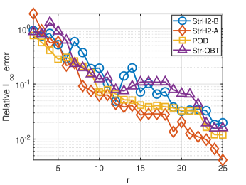
VII-A New England test system
The model has order in the original second-order coordinates (2). We choose in (60). We apply both formulations of StrH2 in Algorithm 3 (StrH2-A and StrH2-B), Str-QBT, and POD; and reduce the order to . In Figure 1, the relative error with vs. reduction order is depicted for each method. The figure shows that for the majority of values, StrH2-A yields the lowest relative error. We note that this is the best case scenario for POD since the reduced model is tested with the same input that is used to train POD.
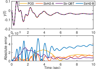
For a more detailed comparison, in Figure 2, the output of the original and all the reduced order models of order (at which the relative error due to StrH2-A drops below ), and the corresponding absolute error, , are depicted. This figure supports the earlier observation that StrH2-A approximates the original model with a better accuracy compared to POD and Str-QBT.
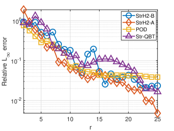
To investigate the robustness of the algorithms to variations in the input, we slightly perturb the input and repeat the same model reduction procedures as before. One might view this perturbation to the input as if the operation conditions are slightly varied. We perturb the input only by . Note that the choice of input has never entered the proposed algorithm or Str-QBT; however it is used to train the POD model. Figures 3 shows the relative error as varies for this slightly varied input. As in the previous case, StrH2-A outperforms the other methods. We also observe that the relative errors for the POD reduced models stagnate after , i.e., not much further improvements, while StrH2-A and StrH2-B, and Str-QBT approximate the original model with almost the same accuracy as in the earlier case. This is expected since the input never entered the model reduction process of the StrH2-A, StrH2-B or Str-QBT. Thus, for this small input variation case, those reduced models provide accurate approximations independent of the input selection as in the linear case.
VII-B IEEE 118 bus system
The second-order model (2) in this case has . We choose and apply StrH2-A, StrH2-B and POD for . We use . Str-QBT has been skipped due to its poor performance in this example. The relative output error (101) vs. is depicted in Figure 4(a). Although POD yields a lower error (the testing input is the same as the training input for POD), StrH2-A has an acceptable accuracy as POD.
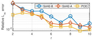
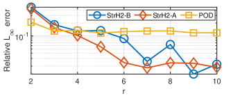
As in the previous example, to test the robustness of the algorithms in the presence of a variation in the input, we slightly perturb the input by . As one can observe in Figure 4(b), both StrH2-A and StrH2-B outperform POD. Also as in the previous example, the relative errors for the POD reduced models do not show further improvements after , while both StrH2 formulations approximate the original model with similar accuracy as in the former case.
VIII Conclusion
We have developed a structure-preserving system-theoretic MOR technique for nonlinear power grid networks. We lifted the original nonlinear model to its equivalent quadratic form in order to employ Q-IRKA as an intermediate stage of our MOR framework. We have shown that the model reduction bases obtained by Q-IRKA have a specific subspace structure that can be exploited to construct the desired reduction basis for reducing the original nonlinear model. This reduction basis has led to a reduced model that preserved the physically meaningful second-order structure of the original model. We have illustrated the effectiveness of our proposed approach via two numerical examples.
References
- [1] U. D. Annakkage, N. K. C. Nair, Y. Liang, A. M. Gole, V. Dinavahi, B. Gustavsen, T. Noda, H. Ghasemi, A. Monti, M. Matar, R. Iravani, and J. A. Martinez. Dynamic system equivalents: A survey of available techniques. IEEE Transactions on Power Delivery, 27(1):411–420, 2012.
- [2] A. C. Antoulas, C. Beattie, and S. Güğercin. Interpolatory methods for model reduction. Computational Science and Engineering 21. SIAM, Philadelphia, 2020.
- [3] P. Benner and T. Breiten. Interpolation-based -model reduction of bilinear control systems. SIAM Journal on Matrix Analysis and Applications, 33(3):859–885, 2012.
- [4] P. Benner and T. Breiten. Two-sided projection methods for nonlinear model order reduction. SIAM Journal on Scientific Computing, 37(2):B239–B260, 2015.
- [5] P. Benner and P. Goyal. Balanced truncation model order reduction for quadratic-bilinear control systems. e-print 1705.00160, arXiv, 2017.
- [6] P. Benner, P. Goyal, and S. Gugercin. -quasi-optimal model order reduction for quadratic-bilinear control systems. SIAM Journal on Matrix Analysis and Applications, 39(2):983–1032, 2018.
- [7] B. Besselink, U. Tabak, A. Lutowska, N. van de Wouw, H. Nijmeijer, D.J. Rixen, M.E. Hochstenbach, and W.H.A. Schilders. A comparison of model reduction techniques from structural dynamics, numerical mathematics and systems and control. Journal of Sound and Vibration, 332(19):4403–4422, 2013.
- [8] D. Chaniotis and M. A. Pai. Model reduction in power systems using Krylov subspace methods. IEEE Transactions on Power Systems, 20(2):888–894, 2005.
- [9] S. Chaturantabut and D. C. Sorensen. Nonlinear model reduction via discrete empirical interpolation. SIAM Journal on Scientific Computing, 32(5):2737–2764, 2010.
- [10] X. Cheng and J. M. A. Scherpen. Clustering approach to model order reduction of power networks with distributed controllers. Advances in Computational Mathematics, 44(6):1917–1939, Dec 2018.
- [11] A. Cherid and M. Bettayeb. Reduced-order models for the dynamics of a single-machine power system via balancing. Electric Power Systems Research, 22(1):7 – 12, 1991.
- [12] J. H. Chow. Power system coherency and model reduction, volume 84. Springer, 2013.
- [13] J. H. Chow, J. R. Winkelman, M. A. Pai, and P. W. Sauer. Singular perturbation analysis of large-scale power systems. International Journal of Electrical Power & Energy Systems, 12(2):117 – 126, 1990.
- [14] C. Gu. Qlmor: A projection-based nonlinear model order reduction approach using quadratic-linear representation of nonlinear systems. IEEE Transactions on Computer-Aided Design of Integrated Circuits and Systems, 30(9):1307–1320, 2011.
- [15] M. Hinze and S. Volkwein. Proper orthogonal decomposition surrogate models for nonlinear dynamical systems: Error estimates and suboptimal control. In P. Benner, D. C. Sorensen, and V. Mehrmann, editors, Dimension Reduction of Large-Scale Systems, pages 261–306. Springer Berlin Heidelberg, 2005.
- [16] T. Ishizaki, K. Kashima, A. Girard, J. Imura, L. Chen, and K. Aihara. Clustered model reduction of positive directed networks. Automatica, 59:238 – 247, 2015.
- [17] T. G. Kolda and B. W. Bader. Tensor decompositions and applications. SIAM Review, 51(3):455–500, 2009.
- [18] J. Leung, M. Kinnaert, J. Maun, and F. Villella. Model reduction of coherent LPV models in power systems. In 2019 IEEE Power Energy Society General Meeting (PESGM), pages 1–5, 2019.
- [19] Y. Levron and J. Belikov. Reduction of power system dynamic models using sparse representations. IEEE Transactions on Power Systems, 32(5):3893–3900, 2017.
- [20] S. Liu. Dynamic-data driven real-time identification for electric power systems. PhD thesis, University of Illinois at Urbana-Champaign, 2009.
- [21] M. H. Malik, D. Borzacchiello, F. Chinesta, and P. Diez. Reduced order modeling for transient simulation of power systems using trajectory piece-wise linear approximation. Advanced Modeling and Simulation in Engineering Sciences, 3(1):31, Dec 2016.
- [22] G. P. McCormick. Computability of global solutions to factorable nonconvex programs: Part i—convex underestimating problems. Mathematical programming, 10(1):147–175, 1976.
- [23] P. Mlinarić, S. Grundel, and P. Benner. Efficient model order reduction for multi-agent systems using QR decomposition-based clustering. In Proceedings of 54th IEEE Conference on Decision and Control, pages 4794–4799, 2015.
- [24] P. Mlinarić, T. Ishizaki, A. Chakrabortty, S. Grundel, P. Benner, and J. Imura. Synchronization and aggregation of nonlinear power systems with consideration of bus network structures. In 2018 European Control Conference (ECC), pages 2266–2271, 2018.
- [25] T. Nishikawa and A. E Motter. Comparative analysis of existing models for power-grid synchronization. New Journal of Physics, 17(1):015012, 2015.
- [26] D. Osipov and K. Sun. Adaptive nonlinear model reduction for fast power system simulation. IEEE Transactions on Power Systems, 33(6):6746–6754, 2018.
- [27] M. A. Pai and R. P. Adgaonkar. Singular perturbation analysis of nonlinear transients in power systems. In 1981 20th IEEE Conference on Decision and Control including the Symposium on Adaptive Processes, pages 221–222, 1981.
- [28] P. A. Parrilo, S. Lall, F. Paganini, G. C. Verghese, B. C. Lesieutre, and J. E. Marsden. Model reduction for analysis of cascading failures in power systems. In Proceedings of the 1999 American Control Conference (Cat. No. 99CH36251), volume 6, pages 4208–4212, 1999.
- [29] E. Purvine, E. Cotilla-Sanchez, M. Halappanavar, Z. Huang, G. Lin, S. Lu, and S. Wang. Comparative study of clustering techniques for real-time dynamic model reduction. Statistical Analysis and Data Mining: The ASA Data Science Journal, 10(5):263–276, 2017.
- [30] J. Qi, J. Wang, H. Liu, and A. D. Dimitrovski. Nonlinear model reduction in power systems by balancing of empirical controllability and observability covariances. IEEE Transactions on Power Systems, 32(1):114–126, 2017.
- [31] E. Qian, B. Kramer, B. Peherstorfer, and K. Willcox. Lift & learn: Physics-informed machine learning for large-scale nonlinear dynamical systems. Physica D: Nonlinear Phenomena, 406:132401, 2020.
- [32] A. Ramirez, A. Mehrizi-Sani, D. Hussein, M. Matar, M. Abdel-Rahman, J. Jesus Chavez, A. Davoudi, and S. Kamalasadan. Application of balanced realizations for model-order reduction of dynamic power system equivalents. IEEE Transactions on Power Delivery, 31(5):2304–2312, 2016.
- [33] T. K.S. Ritschel, F. Weiß, M. Baumann, and S. Grundel. Nonlinear model reduction of dynamical power grid models using quadratization and balanced truncation. at - Automatisierungstechnik, 68(12):1022–1034, 2020.
- [34] B. Safaee and S. Gugercin. Data-driven modeling of power networks. In 2021 60th IEEE Conference on Decision and Control (CDC), pages 4236–4241, 2021.
- [35] B. Safaee and S. Gugercin. Structure-preserving model reduction of parametric power networks. In 2021 American Control Conference (ACC), pages 1824–1829, 2021.
- [36] C. Sturk, L. Vanfretti, Y. Chompoobutrgool, and H. Sandberg. Coherency-independent structured model reduction of power systems. IEEE Transactions on Power Systems, 29(5):2418–2426, 2014.
- [37] A. van der Schaft. On model reduction of physical network systems. In Proceedings of 21st International Symposium on Mathematical Theory of Networks and Systems (MTNS), pages 1419–1425, 2014.
- [38] C. Wang, H. Yu, P. Li, C. Ding, C. Sun, X. Guo, F. Zhang, Y. Zhou, and Z. Yu. Krylov subspace based model reduction method for transient simulation of active distribution grid. In 2013 IEEE Power Energy Society General Meeting, pages 1–5, 2013.
- [39] C. Wang, H. Yu, P. Li, J. Wu, and C. Ding. Model order reduction for transient simulation of active distribution networks. IET Generation, Transmission & Distribution, 9:457–467(10), April 2015.
- [40] S. Wang, S. Lu, G. Lin, and N. Zhou. Measurement-based coherency identification and aggregation for power systems. In 2012 IEEE Power and Energy Society General Meeting, pages 1–7, 2012.
- [41] S. Wang, S. Lu, N. Zhou, G. Lin, M. Elizondo, and M. A. Pai. Dynamic-feature extraction, attribution, and reconstruction (DEAR) method for power system model reduction. IEEE Transactions on Power Systems, 29(5):2049–2059, 2014.
- [42] H. Zhao, X. Lan, and H. Ren. Nonlinear power system model reduction based on empirical gramians. Journal of Electrical Engineering, 68(6):425 – 434, 2017.
- [43] H. S. Zhao, N. Xue, and N. Shi. Nonlinear Dynamic Power System Model Reduction Analysis Using Balanced Empirical Gramian. Applied Mechanics and Materials, 448-453:2368–2374, October 2013.
- [44] R. D. Zimmerman and C. E. Murillo-Sánchez. Matpower 6.0 user’s manual. Power Systems Engineering Research Center, 9, 2016.
- [45] R. D. Zimmerman, C. E. Murillo-Sánchez, and R. J. Thomas. Matpower: Steady-state operations, planning, and analysis tools for power systems research and education. IEEE Transactions on Power Systems, 26(1):12–19, 2010.