Structure of Quantum Mean Force Gibbs States for Coupled Harmonic Systems
Abstract
An open quantum system interacting with a heat bath at given temperature is expected to reach the mean force Gibbs (MFG) state as a steady state. The MFG state is given by tracing out the bath degrees of freedom from the equilibrium Gibbs state of the total system plus bath. When the interaction between the system and the bath is not negligible, it is different from the usual system Gibbs state obtained from the system Hamiltonian only. Using the path integral method, we present the exact MFG state for a coupled system of quantum harmonic oscillators in contact with multiple thermal baths at the same temperature. We develop a nonperturbative method to calculate the covariances with respect to the MFG state. By comparing them with those obtained from the system Gibbs state, we find that the effect of coupling to the bath decays exponentially as a function of the distance from the system-bath boundary. This is similar to the skin effect found recently for a quantum spin chain interacting with an environment. Using the exact results, we also investigate the ultrastrong coupling limit where the coupling between the system and the bath gets arbitrarily large and make a connection with the recent result found for a general quantum system.
I Introduction
In the standard theory of thermodynamics the interaction between a system and its environment is assumed to be weak. However, for systems with decreasing sizes Jarzynski (2017) or for quantum mechanical systems Ford et al. (1985), the interaction cannot be neglected. This consideration has led to the recent development of strong coupling thermodynamics Campisi et al. (2009); Gelin and Thoss (2009); Subaşı et al. (2012); Seifert (2016); Jarzynski (2017); Strasberg and Esposito (2017); Aurell (2017); Miller (2018); Hsiang and Hu (2018); Perarnau-Llobet et al. (2018); Talkner and Hänggi (2020); Rivas (2020); Anto-Sztrikacs et al. (2023); Kaneyasu and Hasegawa (2023); Diba et al. (2024). The mean force Gibbs (MFG) state Trushechkin et al. (2022); Cresser and Anders (2021); Chiu et al. (2022) and the associated Hamiltonian of mean force Kirkwood (1935); Grabert et al. (1984); Hilt et al. (2011); Miller (2018); Timofeev and Trushechkin (2022) play a central role in the theory of strong coupling thermodynamics. The MFG state describes the equilibrium state of the system interacting with a thermal bath at given temperature. When the interaction between the system and the bath is not negligible, the MFG state deviates from the usual system Gibbs state which is described by the system Hamiltonian only Trushechkin et al. (2022), and the Hamiltonian of mean force is different from the system Hamiltonian Hilt et al. (2011).
Despite the importance in strong coupling thermodynamics, explicit evaluation of the quantum MFG state turns out to be quite difficult. Exact results are known only for simple limited cases Grabert et al. (1984); Hilt et al. (2011) of a damped harmonic oscillator described by the Caldeira-Leggett model Caldeira and Leggett (1983). Recently, the MFG state for a general quantum system interacting with a bosonic environment was obtained in both weak and ultrastrong coupling limits Cresser and Anders (2021). The ultrastrong coupling limit of the MFG state obtained in Ref. Cresser and Anders (2021) is quite interesting as it is characterized by a diagonal projection of the system Hamiltonian onto the eigenstates of the system operator which couples to the environment. In order to gain further understanding of quantum thermodynamics beyond weak coupling, it would be useful to have explicit expressions of the MFG state of a more general quantum system which covers the range of the coupling strength from weak to ultrastrong. One of the purposes of this paper is to provide such examples of the quantum MFG state.
Another aspect of the MFG state which has not been investigated as yet is its spatial structure. For an open quantum system with spatial extent, only a part of the system is directly coupled to the heat bath. Therefore, the MFG state as an equilibrium state is expected to exhibit a spatial structure reflecting this local coupling. Recently, in Ref. Burke et al. (2024), the Hamiltonian of mean force of a spin chain interacting with its environment was studied numerically. The results show a kind of skin effect where the effect of the coupling to the environment decays exponentially as one moves away from the system-environment boundary. This suggests that the effect of the local coupling to the environment on the equilibrium state of the system is confined to the vicinity of the point of contact with the environment.
In this paper, we present calculations leading to the MFG state of a coupled system of quantum mechanical harmonic oscillators interacting with multiple thermal baths maintained at given temperature. This is an exact result which covers the range of the coupling strength to the heat baths from weak to ultrastrong. We consider an open quantum system of coupled oscillators described by the Caldeira-Leggett type Hamiltonian Caldeira and Leggett (1983) where only parts of the system are coupled with the baths. By explicitly evaluating the path integrals involved in tracing out the bath degrees of freedom, we present a formalism of obtaining the exact MFG state. Being a Gaussian state, the MFG state is completely described by its covariances. We present a nonperturbative method to evaluate the covariances with respect to the MFG state. By studying the difference in the covariances obtained with respect to the MFG and the system Gibbs states, we show how the local nature of the coupling to the bath shows up in the MFG state. We find that there is a skin effect similar to that found in Ref. Burke et al. (2024), where the effect of the coupling to the heat bath decays exponentially as a function of the distance from the system-bath boundary. Using the exact expressions, we also explore the ultrastrong coupling regime. We find that the expression found in Ref. Cresser and Anders (2021) for this limit is still valid even in the present case where the coupling system operator is local and has a continuous spectrum.
In the following section, we present a general formalism for the calculation of the MFG state of coupled harmonic systems using the path integral method. In Sec. III, we focus on the case where the system is in contact with a single heat bath. Using a specific example of a ring of coupled oscillators, we present detailed expressions for the exact MFG covariances and study their ultrastrong coupling limit. We then generalize to the case where the system is in contact with two or more baths at the same temperature in Sec. IV. Finally. we conclude with discussion.
II MFG state for coupled harmonic systems from path integral
An open quantum system in contact with a thermal bath is expected to approach in the long time limit its stationary state described by the MFG state Subaşı et al. (2012). We consider a quantum mechanical system described by the Hamiltonian interacting with the bath given by . The total Hamiltonian is written as
| (1) |
where the interaction between the system and the bath is governed by . The MFG state is defined by
| (2) |
which is obtained by the partial trace of the equilibrium state of the total system with . When the interaction between the system and bath is not negligible, the MFG state is in general different from the usual system Gibbs state
| (3) |
given by the system Hamiltonian only.
We consider a collection of quantum harmonic oscillators of equal mass . The coupling among these oscillators is described by a symmetric positive definite matrix . The system is described by the Hamiltonian
| (4) |
where and are the position and momentum operators of the -th oscillator, respectively.
We consider the case where only a part of the system is in contact with a collection of heat baths labelled by . We set up a Caldeira-Leggett model Caldeira and Leggett (1983) where each bath is composed of harmonic oscillators with mass and frequency . The Hamiltonian for the heat baths and their interaction with the system can be written as
| (5) | ||||
where and are the momentum and position operators for the oscillators in the bath , respectively. Here the index runs through a subset of such that the oscillator described by the position is coupled with the oscillators in the -th bath with the coupling constant . The distribution of the -th bath modes is conveniently described by the spectral function
| (6) |
We first write the matrix element of using Euclidian path integrals as
| (7) |
where the system Euclidian action is given by
| (8) |
with the matrix notation and . The remaining actions for the bath and the interaction are given respectively by
| (9) |
and
| (10) | |||
with
| (11) |
The matrix element of the MFG state is obtained by tracing over the bath variables. This type of path integral is well-known in the study of the quantum Brownian motion Grabert et al. (1988). The path integral over the bath variables results in the so-called Feynman-Vernon influence functional Feynman and Vernon (1963); Grabert et al. (1988); Weiss (2012). In our case, we can easily modify it to the imaginary time path integral. As a result, we have the influence functional obtained by tracing out the -th bath as
| (12) |
where
| (13) |
Now the matrix element of the MFG state with respect to the system position variables is given by
| (14) |
where with . We note that we can rewrite Eq. (12) as (see Appendix A)
| (15) |
where is defined as a Fourier series expansion in the interval as
| (16) |
with the Matsubara frequency and
| (17) |
Since the path integral in Eq. (14) is Gaussian, it can be evaluated by considering the stationary path and the fluctuation around it. The path integral over the fluctuation will give a constant independent of the endpoints, which can be determined later from the normalization of Grabert et al. (1988). The stationary path is determined from
| (18) |
for . This is to be solved with the boundary conditions and . The solution can be conveniently obtained in terms of the Fourier series expansion
| (19) |
The detailed procedure is given in Appendix B. The solution for the Fourier modes in a matrix form are given by
| (20) |
where the matrices
| (21) |
and
| (22) |
Here is a diagonal matrix whose diagonal element is equal to given in Eq. (17) if belongs to the set and is equal to zero otherwise.
If we insert the solution Eq. (20) with Eq. (19) into the expression of the MFG state, Eq. (14), we obtain (see Appendix C)
| (23) |
where
| (24) |
The overall constant is determined from the normalization
| (25) |
which gives
| (26) |
The MFG state is Gaussian and characterized by the following covariance matrices, which can easily be calculated as
| (27) |
| (28) |
and
| (29) |
III System in Contact with a single heat bath
In this section, using the general formalism developed above, we develop a nonperturbative method to evaluate matrix Green’s function in Eq. (21). To do this, we first focus on coupled harmonic oscillators one end of which is in contact with a heat bath at inverse temperature . In the notation of Eq. (5), we take , that is the oscillator is interacting with the heat bath. Then the only non-vanishing matrix element of which appears in Eq. (21) is given by . Here we have dropped the index in the definition of in Eq. (17) as there is only one bath.
We note that the calculation of the MFG state comes down to evaluating the Green’s function in Eq. (21). A convenient way to do this to express in terms of , which is the Green’s function in the absence of coupling to the bath. If we use in Eq. (23), then we can get the matrix element of the system Gibbs state . We note that can be obtained by diagonalizing . Once we have , we can write
| (30) | ||||
Since the only non-vanishing element of is , we can write
| (31) |
By summing the infinite series, we thus have
| (32) |
where
| (33) |
For later purpose, we rewrite Eq. (33) as
| (34) |
using the matrix with only one nonvanishing element defined by
| (35) |
Another way of writing the full Green’s function is
| (36) | |||
We can then use this equation to obtain the expressions for the covariances with respect to the MFG state in Eqs (27) and (28) as
| (37) |
and
| (38) |
where the summation is now over positive frequencies .
III.1 Example: Chain of Harmonic Oscillators in Contact with a Heat Bath
In this subsection, we apply the method developed in the previous section to a chain of coupled oscillators one end of which is in contact with a heat bath. We consider a system described by Hamiltonian
| (39) |
The parameter describes the coupling between the neighboring oscillators. For convenience, we assume that the system satisfies the periodic boundary condition, . The oscillators thus form a ring (see Fig. 1 (a) for schematic description). The matrix in Eq. (4) is given by
| (40) |
where
| (41) |
As shown in Appendix D, the eigenvalues of are given by , , where
| (42) |
Note that there are two-fold degeneracies as . For stability we require . The eigenvectors of can be used to construct an orthogonal matrix , which diagonalizes as . We therefore have
| (43) | |||
In Appendix D, we present explicit eigenvectors and consequently which diagonalizes and .
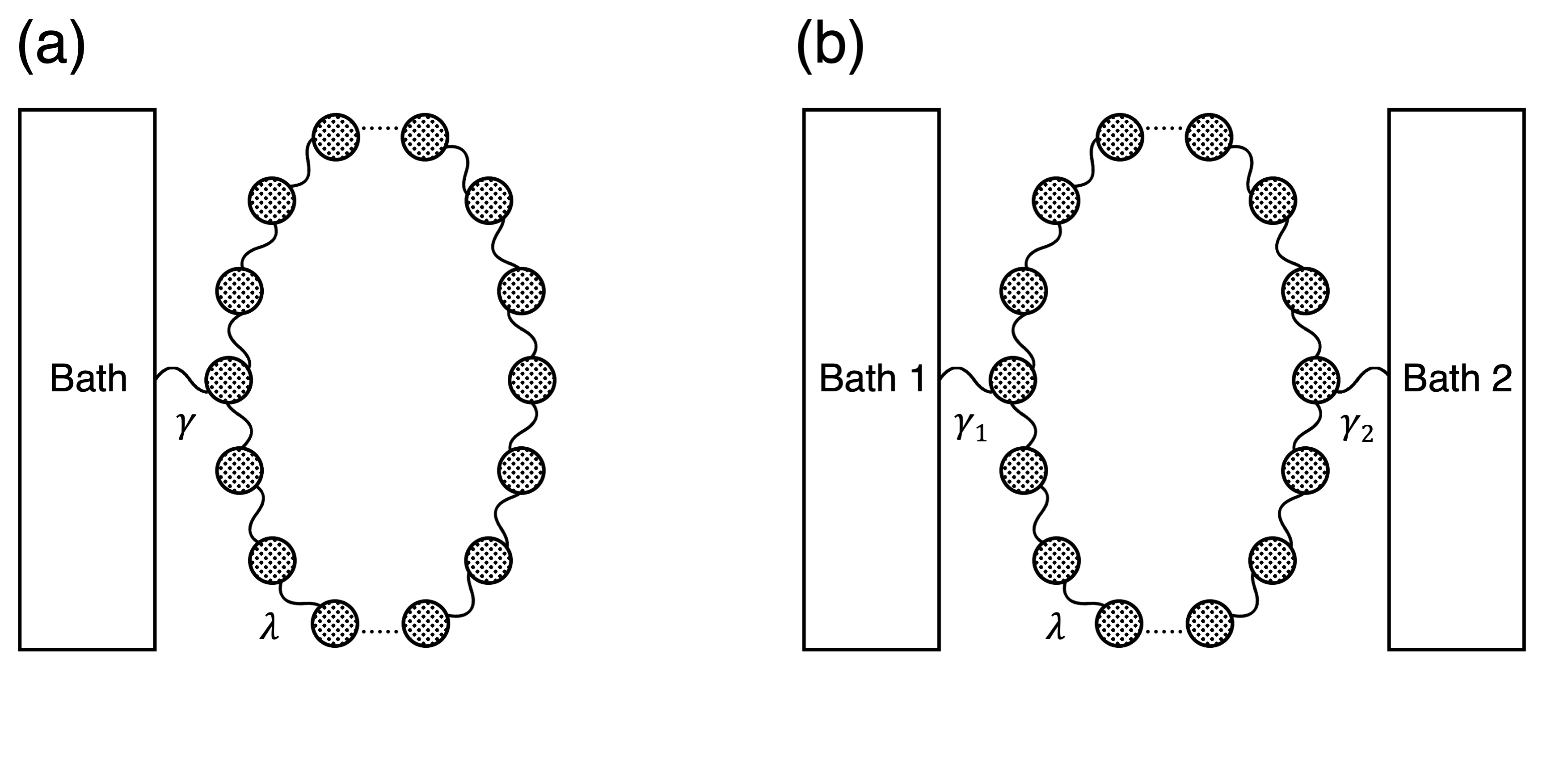
Now the full Green’s function in the presence of the coupling to the bath can be obtained using Eq. (32). The effect of coupling to the bath is characterized by in Eq. (17) and the bath spectral density in Eq. (6). We will again drop the index as there is only one bath. We consider an Ohmic bath with the cutoff and the coupling strength , which is given by
| (44) |
Putting this into Eq. (17), we have
| (45) |
In the following, we present explicit expressions for the MFG state for general values of . As we have seen above in Eqs. (27) and (28), the MFG state is completely characterized by its covariances. First, using the eigenvectors obtained in Appendix D and Eq. (43), we can write
| (46) |
We then obtain the covariances with respect to the system Gibbs state , which we denote by . This can be done by using Eqs. (27) and (28) with replaced by . Using the summation formula
| (47) |
we obtain
| (48) |
For the momentum covariances, we first note from Eq. (43) that
| (49) |
We have from Eq. (28)
| (50) |
Now the covariances with respect to the MFG state can be obtained from the full Green’s function in Eq. (32) with Eq. (33). We therefore have
| (51) | |||
| (52) |
where the differences compared to those obtained with respect to the system Gibbs state are given in terms of in Eq. (33) by
| (53) | |||
| (54) |
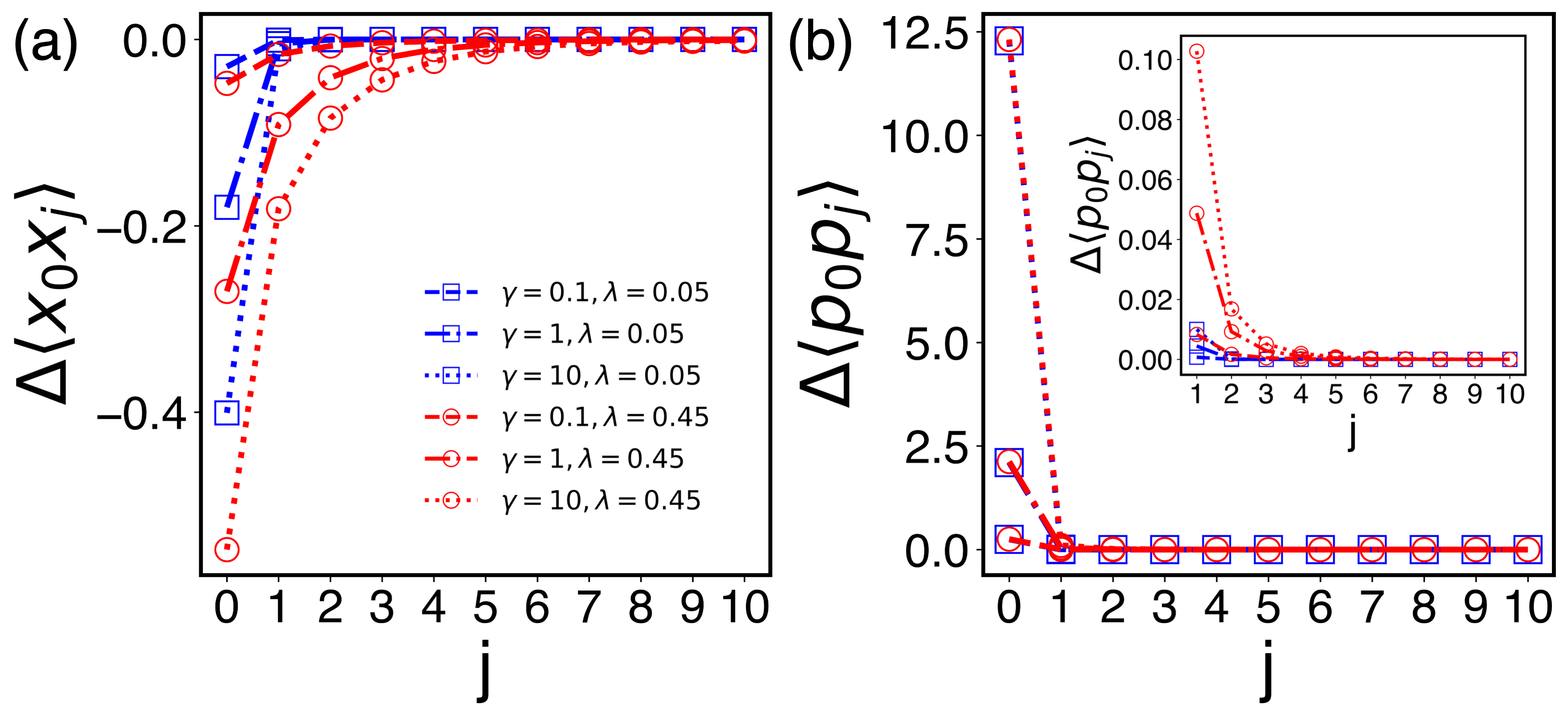
We evaluate the infinite sums in Eqs. (53) and (54) numerically and calculate the covariances with respect to the MFG state. For the numerical calculations, we present and in units of and , respectively. In Figs. 2 and 3, we show the results for and calculated with respect to the MFG state and compare them with those obtained from the system Gibbs state for various values of the coupling strength (in the unit of ) to the bath and of the inter-oscillator coupling constant (in the unit of ). The calculations were done for a ring of coupled oscillators where oscillator is coupled with the heat bath at inverse temperature . We take the Ohmic bath described by Eqs. (44) and (45) with (in the unit of ).
At relatively high temperature, (The inverse temperature is in the unit of .), Fig. 2 (a) shows that exhibits very little variation compared to those obtained from the system Gibbs state, which is independent of (see Eq. (48)). The small difference between the MFG and the system Gibbs averages occurs only near the contact point between the system and the bath. On the other hand, the momentum covariance shows a different behavior as one can see from Fig. 2 (b). The value right at the point of contact with the bath increases quite rapidly as the coupling strength to the bath increases. As we will see below in the next subsection, this is a characteristic behavior of a quantum system where the coupling between the position operators of the system and the heat bath gets stronger. As we can see in the inset of the same figure, away from the point of contact, the effect of the coupling to the bath quickly disappears as in the position covariance.
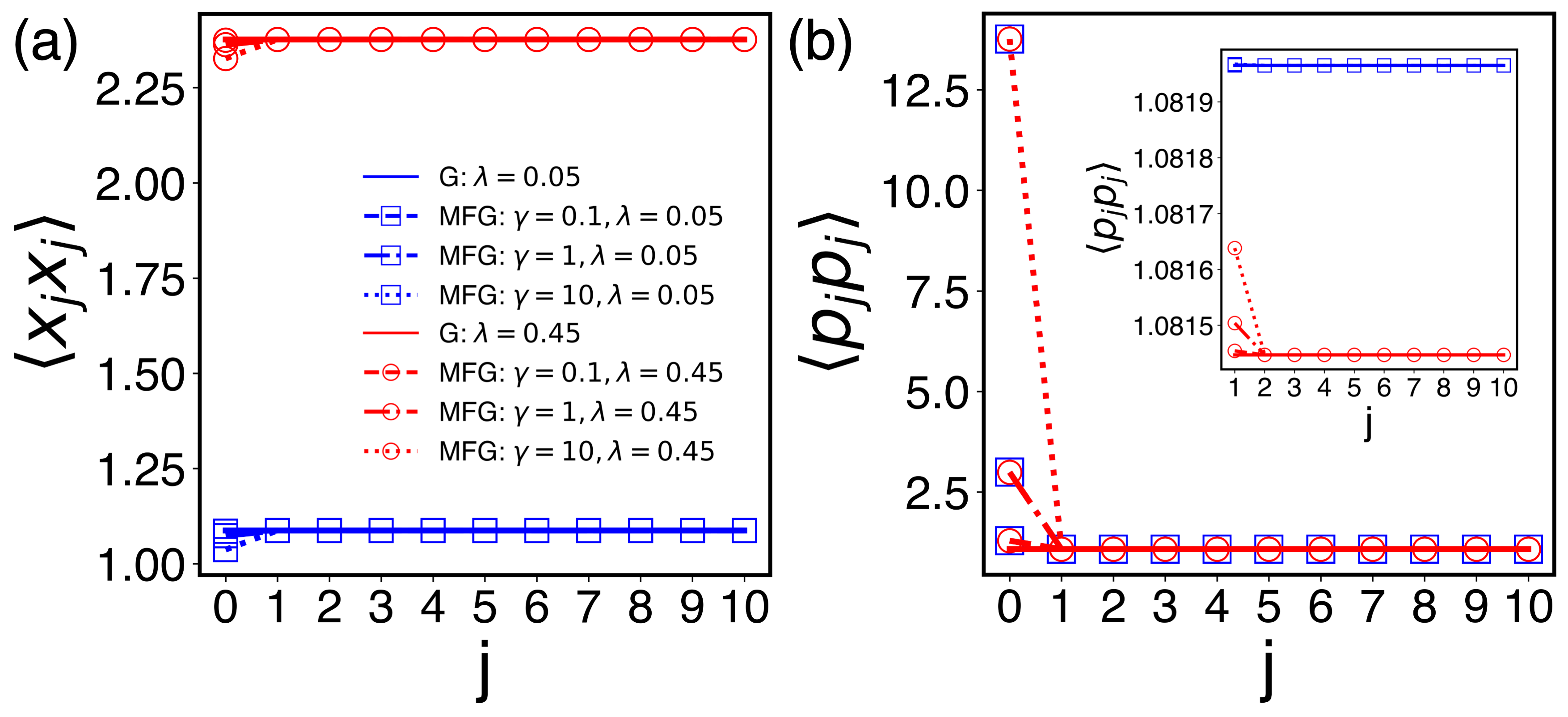
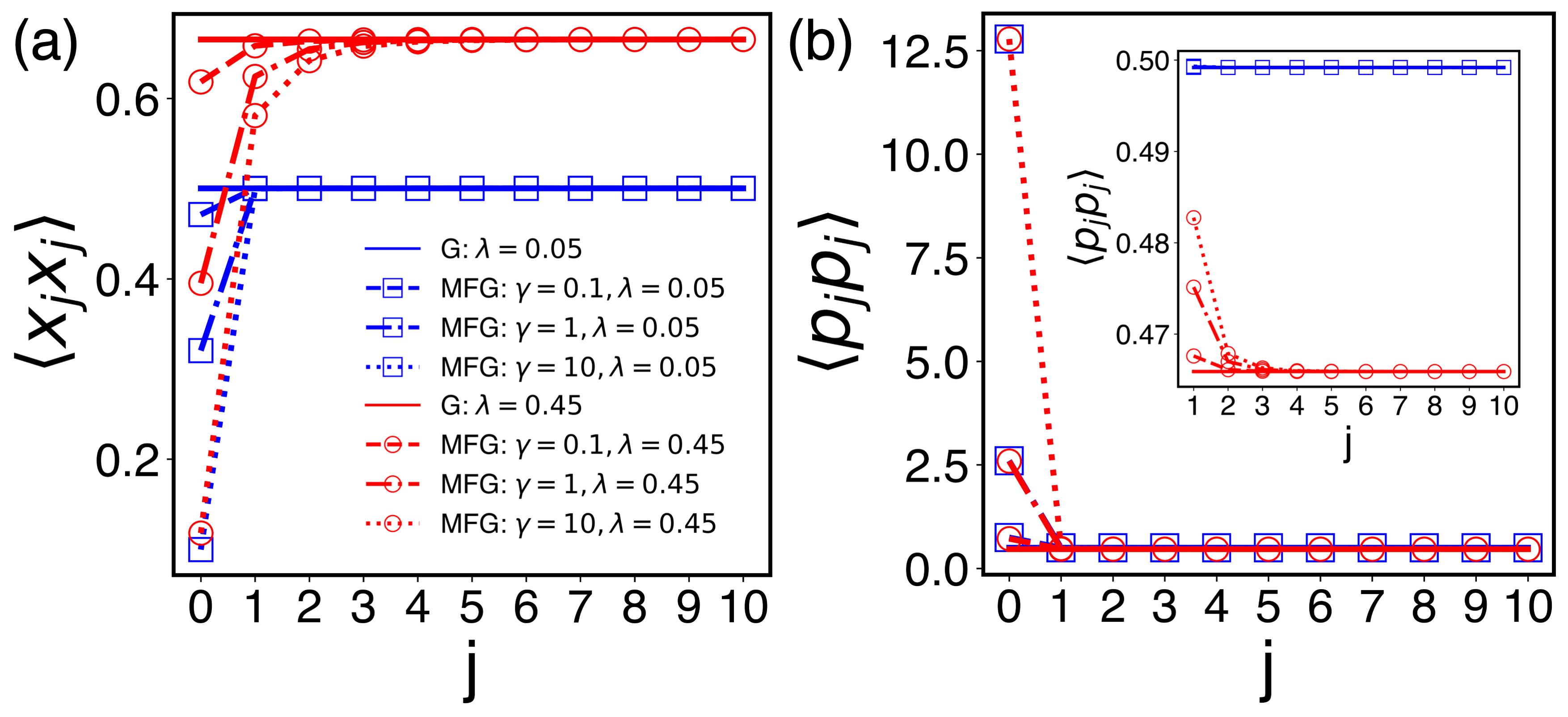
At lower temperatures, the effect of the coupling to the bath in is more prominent as we can see in Fig. 3 (a) at the inverse temperature . The effect, however, disappears as we move away from the point of contact with the bath. In fact, at lower temperatures , we find that the difference defined in Eq. (51) is well described by an exponential decay with the characteristic length . This is quite similar to the skin effect found in Ref. Burke et al. (2024), where the effect of coupling to the environment decays exponentially with the distance from the system-environment boundary. In Fig. 4 (a), we plot the skin depth as a function of the inter-oscillator coupling for various values of the temperature and the coupling strength to the bath. We note that is quite small () even at low temperatures and strong system-bath couplings, and that it shows only a moderate increase as a function of and . A somewhat surprising result is that the effect of the bath measured in terms of is almost independent of the coupling strength to the bath for given values of and . The momentum covariance at lower temperatures, on the other hand, behaves quite similarly to that at higher temperatures as can be seen from Fig. 3 (b). The main feature still is a sharp increase of as increases. The effect of the coupling to the bath quickly disappears as can be seen in the inset of Fig. 3 (b).
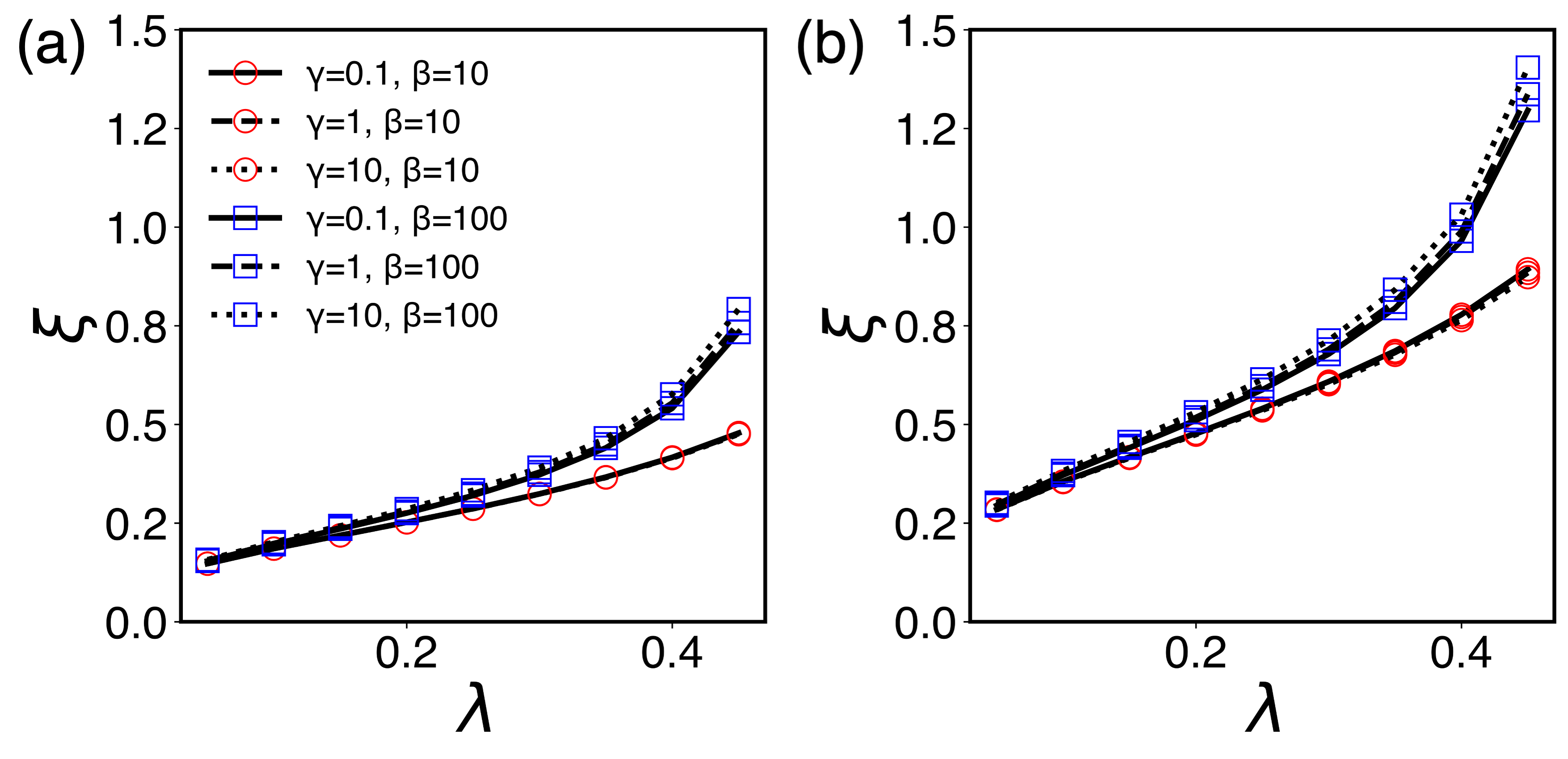
In order to study the effect of the coupling to the bath on the MFG state further, we look at another type of covariances, and , which connect operators at different sites, and compare them with those obtained with respect to the system Gibbs state. We again study the effect of the coupling to the bath using the differences, and between the MFG and the system Gibbs states, which are plotted in Fig. 5 at inverse temperature for oscillators. We note that in this case the system Gibbs averages as well as the MFG ones show a spatial dependence on as one can see from Eqs. (48) and (50). The differences between them, however, show a similar behavior to the previous case of as can be seen from Fig. 5 (a). In fact, we find that is also well described by an exponential decay . We plot the skin depth for this covariance in Fig. 4 (b) for various values of the parameters. We note that the skin depths in this case are slightly bigger than those for , but the overall behavior of as a function of the coupling constants and temperatures is quite similar to the previous case. The main point we make here is that the effect of the heat bath on the equilibrium state measured with in both cases is quite short-ranged reaching only over one site. The difference in the momentum covariance connecting different sites also shows a similar behavior to . Apart from the increasing at as gets bigger, the effect of the coupling to the bath quickly disappears as we move away from the contact point as we can see in Fig. 5 (b).
III.2 The Ultra Strong Coupling (USC) Limit
In this subsection, we investigate the MFG state obtained above, which is an exact result, in the limit when the coupling between the system and the bath is arbitrarily large. This is to make a connection with the ultra strong coupling (USC) limit obtained recently in Ref. Cresser and Anders (2021) of the MFG state for a general system coupled with a bath. If the interaction Hamiltonian between system and bath is given by with a system operator and a bath operator , and the coupling strength , it was shown in Ref. Cresser and Anders (2021) that the MFG state in the limit is diagonal in the eigenstates of . More explicitly, the ultra strong coupling limit is given by Cresser and Anders (2021)
| (55) |
where is the projection operator on the eigenstates of with eigenvalue . In other words, the USC limit is characterized by the effective Hamiltonian of mean force , which is just the system Hamiltonian but projected onto the eigenstates of the system operator taking part in the coupling to the bath.
The reason we study our present system in this limit is twofold. First, for the case of harmonic oscillators, the system operator coupled to the bath is just the position operator at thus has a continuous spectrum. Therefore, the USC limit of the exact MFG state for the quantum harmonic oscillators can provide a generalization of Eq. (55) which was originally obtained in Ref. Cresser and Anders (2021) for the coupling system operator with a discrete spectrum to a continuous one.
To illustrate this point, we consider the simplest case of a single () damped harmonic oscillator Grabert et al. (1984); Hilt et al. (2011) in the USC limit. Putting in Eqs. (21), (27) and (28), we have
| (56) | |||
| (57) |
Taking the coupling strength in to infinity (see Eq. (45)), we see that the infinite sum in diverges. We also find that only the term in Eq. (56) survives, which gives as . As can be seen from Eqs. (23), the diverging momentum covariance indicates that the matrix element is proportional to i.e. diagonal in eigenstates of in the USC limit. This point was recognized recently in Ref. Kumar and Ghosh (2024). The actual value of the position covariance in the USC limit indicates that is given by the Gibbs state of an effective Hamiltonian of the form . This is exactly the system Hamiltonian projected onto the position eigenstate as done in Eq. (55). It is, however, different from another form of the USC limit suggested in Refs. Goyal and Kawai (2019); Orman and Kawai (2020), which is equal to in our case. Therefore it would give the position covariance as as one can see from the diagonal element in Eq. (23) with for . But this is clearly in disagreement with the actual USC limit obtained from the exact expression except for very high temperatures.
The second point why we study the USC limit in our model is the following. We note that the USC limit suggested in Eq. (55) is characterized by the effective Hamiltonian which is a diagonal projection onto the eigenstates of the system operator that couples to the bath. In our model, this system operator is only local as only a part of the system couples to the bath. Therefore, using our exact result, we can check whether the USC limit in Eq. (55) still holds for the case where the coupling operator is local in space. To do this we focus on the simplest case , where the positions of the oscillator are and and only is coupled to the bath. The normal mode frequencies from Eq. (42) are and , and from Eq. (46), we have
| (58) | |||
| (59) |
The USC limit of the two-oscillator system is obtained by taking in Eqs. (37) and (38). We have
| (60) | |||
| (61) |
and
| (62) |
For the momentum covariances, we can easily see from Eq. (38) that and as and
| (63) |
We now check whether the USC limit, Eq. (55) conjectured in Ref. Cresser and Anders (2021) is consistent with this large- limit obtained from the exact results. In the present two-oscillator case, the USC limit of Ref. Cresser and Anders (2021) is characterized by the effective Hamiltonian which is a diagonal projection of onto the eigenstates of . As we have seen in the one-oscillator case, it amounts to suppressing in the system Hamiltonian the kinetic energy () of the oscillator in contact with the heat bath. The matrix element of in Eq. (55) is then given by
| (64) | ||||
where the system Euclidian action is given by
| (65) |
with . We can evaluate this path integral by seeking the stationary path solution as done in Sec. II and in Appendices B and C. Detailed calculations are given in Appendix E. We obtain
| (66) |
where
| (67) | |||
| (68) |
and is determined from .
The covariances are now calculated by evaluating Gaussian integrals such as
| (69) |
and
| (70) |
where we have shifted the integration variable in the second integral. Note that these are exactly the same as Eqs. (60) and (61), respectively. The remaining part is given by
| (71) |
We can easily verify that this coincides with Eq. (62). For the momentum covariance, we can see that only the off-diagonal part () is relevant. Therefore, we have
| (72) |
which is just Eq. (63). In summary, we have verified that the USC limit given as Eq. (55) is still valid even if the projection is onto a local system operator.
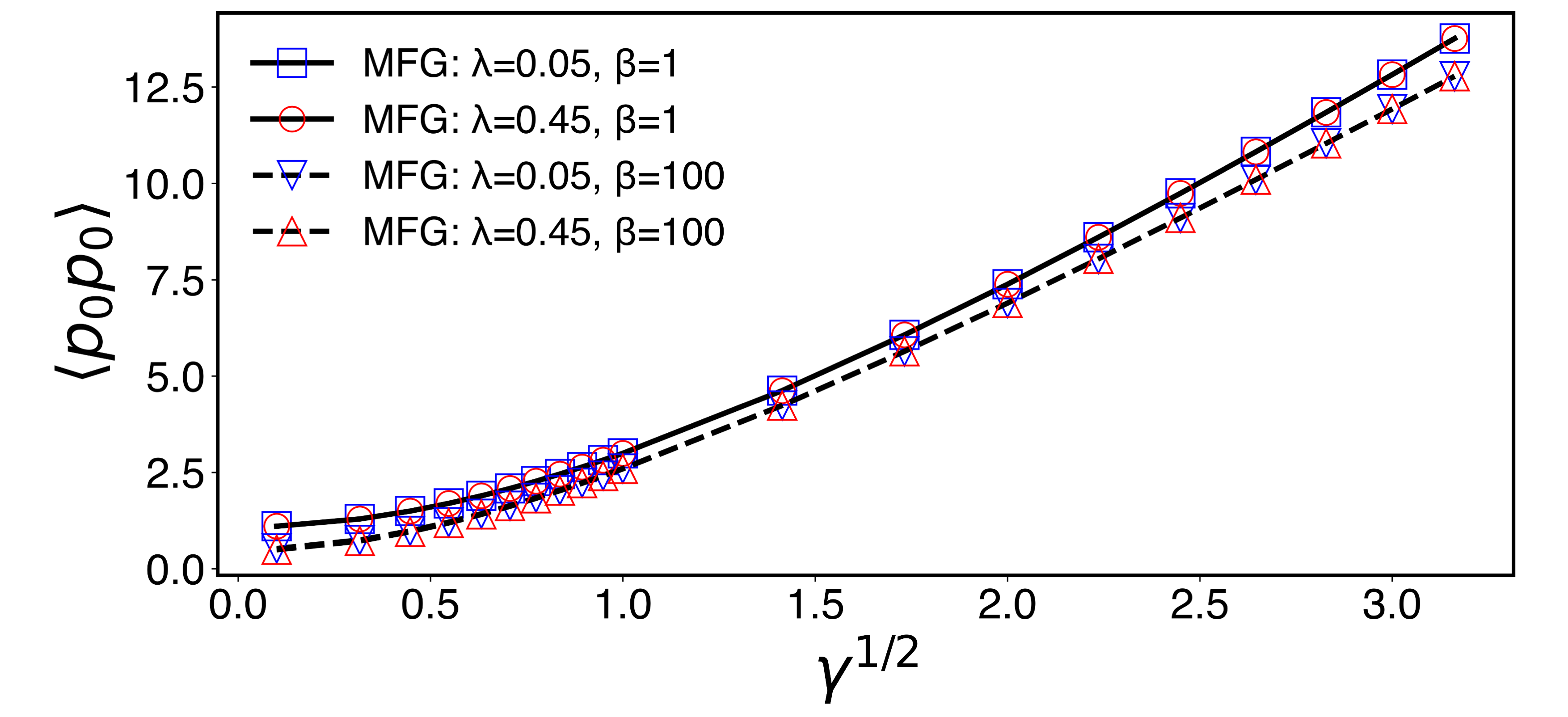
As we have shown, the USC limit is characterized by the diverging momentum covariance at the point of contact with the heat bath. This is related to the projection of the effective Hamiltonian on the space of system local coupling operator in the USC limit. The divergence of as can be made more quantitative as follows. For the case with the Ohmic bath given in Eq. (45), we can actually show that as
| (73) |
The derivation is given in Appendix F. In fact we find that this large- behavior of continues to be true even for general number of oscillators. Figure 6 shows as a function of for oscillators for various temperatures and inter-oscillator coupling constants. For large , it increases with . Therefore, we conclude that in the USC limit goes to infinity, which results in the projection of the MFG state onto the eigenstate of that couples to the heat bath.
IV System in contact with multiple heat baths at the same temperature
In this section, we apply the general formalism developed above to the case where there are multiple heat baths at the same inverse temperature . We first focus on the case where there are two baths and the system makes contact with them at the locations given by . We then generalize to the multiple-bath case. For the two-bath case, the diagonal matrix in Eq. (21) has only two nonzero elements, namely and . For later use, we denote by the matrix composed of these nonzero elements, which belongs to the subspace spanned by .
As in the case of the single bath, we try to express the Green’s function in Eq. (21) in terms of which is obtained in the absence of the coupling to the bath and the correction to it. Now from Eq. (30), we can rewrite this as
| (74) |
where
| (75) |
From the structure of these terms, we realize that all the elements of are zero except when and are equal to or . We again denote this nonzero matrix by . We note that Eq. (74) has the same structure as Eq. (34) for the one-bath case. The only difference is that now contains a nonzero sub-matrix instead of the single nonvanishing component. In order to calculate this , we notice that Eq. (75) can be considered as a relation among matrices , and , the last of which is a matrix composed of with . By summing the infinite series in Eq. (75), we can write
| (76) |
So is obtained by simply inverting the known matrix. The correction term can then be calculated using Eq. (34) with newly obtained .
This procedure can easily be generalized to a system in contact with reservoirs with . All one has to do is to calculate the kernel matrix from Eq. (76) and calculate the Green’s function for the MFG state from Eq. (74).
IV.1 Example: Chain of Harmonic Oscillators in Contact with Two Heat Baths at the Same Temperature
Here we apply this method to the ring of oscillators studied in Sec. III.1. We focus on the case where there are even number of oscillators and the two baths are connected to the oscillators at and . In the present notation, we take and . See Fig. 1 (b) for a schematic diagram describing the situation. We assume that the two baths are described by the Ohmic spectral densities. In particular, we assume that the baths at and are described by and , respectively, which are given by
| (77) |
with in general two distinct coupling strengths and .
In order to calculate in Eq. (76), we first note that in the subspace of
| (78) |
It is then straightforward to evaluate from Eq. (76). From Eqs. (76) and (78), we have
| (79) |
From Eq. (46), we can see that only two of the components of are independent, which we denote by
| (80) | |||
| (81) |
By inverting the above matrix, we obtain
| (82) | |||
| (83) |
and
| (84) |
where
| (85) |
Using these results and Eq. (34), we can write the correction to the system Gibbs state as
| (86) |
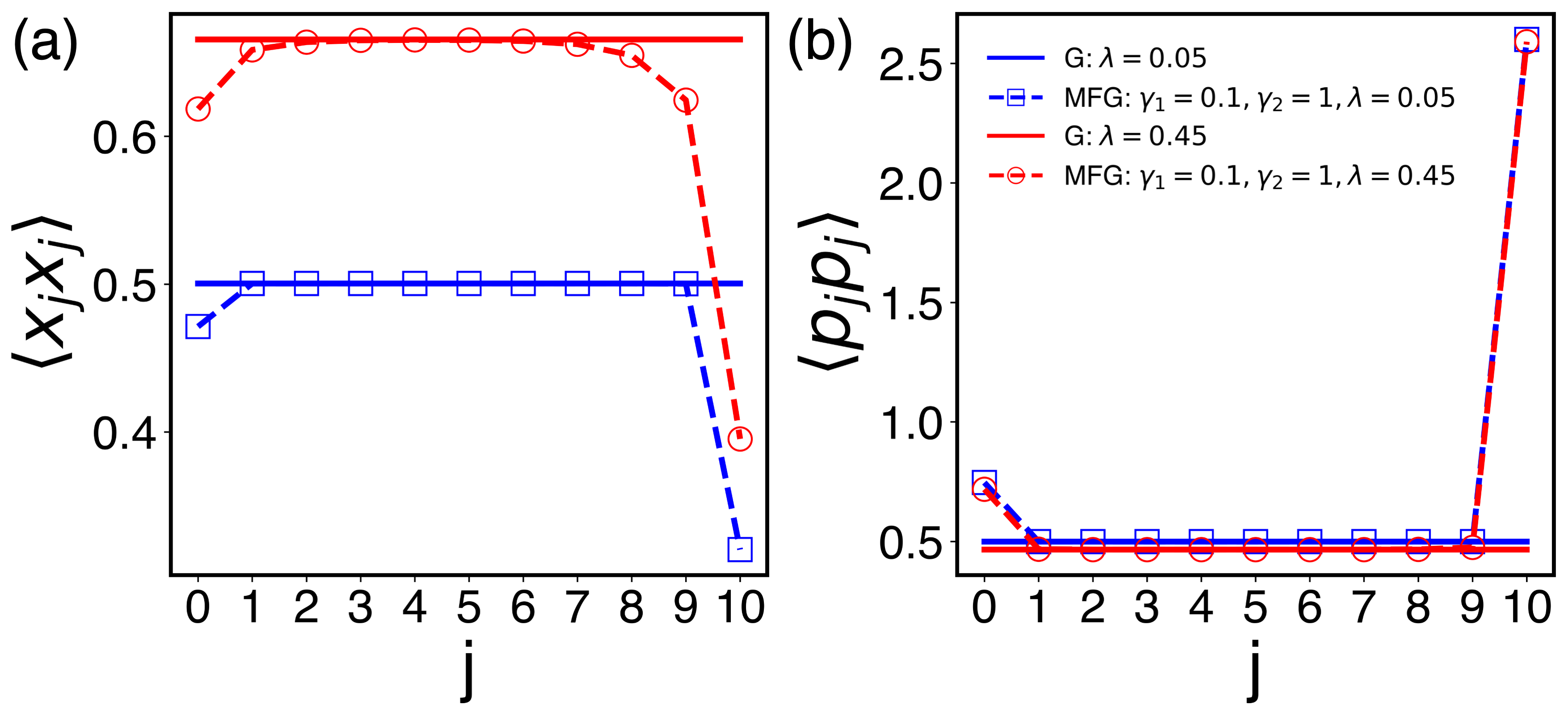
We now calculate the covariances using Eqs. (53) and (54) by evaluating the infinite sums numerically. In Fig. 7, we show results of these calculations for a system coupled to two heat baths maintained at some low temperature with different coupling strengths. As in the one-bath case, the MFG state shows a skin effect for each heat bath, where the effect of the coupling to the bath quickly decreases as one moves away from the contact points. For a relatively large system size , Fig. 7 shows a separate skin effect for each heat bath.
V Discussion and Summary
We have presented a detailed procedure of obtaining the exact quantum MFG state of a coupled harmonic system interacting with multiple heat baths at the same temperature. We have provided a nonperturbative method to calculate the covariances with respect to the MFG state. For the specific examples of the chain of harmonic oscillators, we have calculated these covariances as we vary the physical parameters such as the temperature, the coupling strength to the bath and the inter-oscillator coupling constant and compare them with those calculated with respect to the system Gibbs state. We found that there is a skin effect similar to that found in Ref. Burke et al. (2024), where the effect of the coupling to the bath quickly disappears as a function of the distance of the system-bath boundary. We have also investigated quantitatively the skin depth and found that it is quite short-ranged and insensitive to the coupling strength to the bath. Using these exact results, we were also able to confirm that the ultrastrong coupling limit of the MFG state found recently in Ref. Cresser and Anders (2021) is valid even in the case where the system coupling operator is local and has a continuous spectrum.
An interesting aspect of the MFG state which has not been explored in this paper is its relation to the thermalization of an open quantum system. If we consider the dynamics of an open quantum system coupled with a heat bath, we expect the system reaches the MFG state as a steady state. The dynamics is often described in terms of quantum master equations, most of which are based on weak coupling approximations Breuer and Petruccione (2007). The Lindblad equation Lindblad (1976); Gorini et al. (1976) has been studied extensively as it guarantees the complete positivity. The standard derivation of the Lindblad equation involves a series of weak coupling approximations, which forces the local coupling system operator to be written in terms of eigenoperators with respect to the whole system Hamiltonian Breuer and Petruccione (2007) and in turn makes it global. The global Lindblad equation is often referred as a ultraweak coupling theory Trushechkin et al. (2022) as its steady state is given by the system Gibbs state, which is the zero coupling limit of the MFG state. One can keep the local nature of the coupling system operator in the Lindblad equation Landi et al. (2022). The local Lindblad equation is shown to be consistent with local conservation laws Tupkary et al. (2023) unlike the global one, but the steady state is no longer given by the Gibbs or MFG state Tupkary et al. (2022); Carlen et al. (2024). If we relax the condition of complete positivity, one has the Redfield equation, Redfield (1957) which can again be derived from the weak coupling approximations corresponding to the second-order perturbative expansion in the system-bath coupling. Now, the steady state of the Redfield equation is known to be equal to the perturbative MFG state valid up to the same order of perturbation theory Thingna et al. (2012); Tupkary et al. (2022); Lee and Yeo (2022). However, as in the global Lindblad equation, the coupling system operator becomes global. This seems to be in contrast to our finding here that the local nature of the system operator playing a role in the structure of the MFG state. It would be interesting to see how the structure of the MFG state found in this paper manifest in the steady states of various weak-coupling quantum master equations for an extended system.
Acknowledgements.
This work was supported by NRF grant funded by the Korea government (MSIT) (RS-2023-00276248).Appendix A The Influence Functional
We first write in Eq. (13) which is periodic in the interval as a Fourier series
| (87) |
with . Then using Eq. (13) we have
| (88) |
where and are defined in Eq. (11) and Eq. (17), respectively. Putting this back into Eq. (87) and using the Poisson sum rule, we have
| (89) |
where is given in Eq. (16). We therefore have
| (90) |
Appendix B Stationary Path Solution
We follow closely the procedure described in Ref. Grabert et al. (1988). We solve the stationary path condition Eq. (18) using the Fourier series given in Eq. (19), which is defined outside the interval as well. The derivatives of with respect to then produce singularities at the endpoints , . In order to account for these singularities, we rewrite Eq. (18) as
| (91) | |||
for some constants and to be determined later, where
| (92) |
is the discrete delta function. In terms of the Fourier mode, we have for ,
| (93) |
This equation is to be solved with the boundary condition and . The solution can be written as
| (94) |
where
| (95) |
and is a diagonal matrix with non-vanishing elements only for , that is
| (96) |
The discontinuity of at is responsible for term proportional to . In fact we can easily see that
| (97) |
The discontinuity at can also be read off from Eq. (94) by forming and taking the limit. We first note that for large , . Therefore the term proportional to in Eq. (94) contains a contribution which goes as for large . This kind of contribution when summed over all nonzero signals a discontinuity at . More explicitly, we write a part of obtained from the first term on the right hand side of Eq. (94) as
| (98) |
where and the prime indicates that the absence of the term. When taking the limit, the term in the round parenthesis vanishes as is even in . We also note that a sawtooth wave defined in has a Fourier expansion
| (99) |
Note that the sawtooth wave has a discontinuity as and . Therefore, Eq. (98) becomes as and as . Finally by taking the limit of , we have from Eq. (94)
| (100) | |||
| (101) |
where
| (102) |
Adding these two equations, we have
| (103) |
Inserting Eqs. (103) and (97) into Eq. (94), we have Eq. (20).
Appendix C Evaluation of the MFG State from the Stationary Solution
We write the actions inside the exponential of Eq. (14) using the stationary solution Eq. (20) with Eq. (94). We note that the derivative expressed in terms of the Fourier modes contains the delta function singularities coming from the discontinuities. By removing these singularities and using the matrix notations for Eq. (97) and for Eq. (103), we can write
| (104) | ||||
Then we have
| (105) |
where we have used the fact that is even in and that the terms odd in vanish after the summation. Using Eq. (94), we have
| (106) |
| (107) |
Adding these three contributions in Eq. (14) and recalling the definition of in Eq. (21), we have
| (108) |
Inserting Eqs. (97) and (103) into this, we finally arrive at Eq. (23).
Appendix D Diagonalization of Matrices for a Chain of Oscillators
We first note that the matrices and in Eq. (40) share the same eigenvectors. By direct application, we can check that the eigenvectors of in Eq. (41) are given up to normalization constant in the form Serafini (2017)
| (109) |
for with eigenvalue . The eigenvalue of is then given by Eq. (42). We note that there are two-fold degeneracies as . Below, we construct the orthonormal set of eigenvectors for the cases of even and odd separately.
For odd, the space of is one dimensional with normalized eigenvector
| (110) |
On the other hand, the space of with is doubly degenerate. We can form a linear combination of and which is proportional to to make a real eigenvector for this eigenvalue. These are given by
| (111) |
and
| (112) |
We can easily show that the collection of and for form an orthonormal set. Now we relabel these vectors by using for such that and for . For the remaining part , we assign . Then the set with is the desired orthonormal set of eigenvectors of corresponding to eigenvalue .
Therefore, we can form an orthogonal matrix by putting the eigenvectors on the columns as
| (113) |
This matrix can then be used to diagonalize as .
Using this matrix , we can calculate the zeroth order Green’s function in Eq. (43) as
| (114) | ||||
This can be easily seen to be equivalent to Eq. (46).
The case of even is similar. We first note that the spaces corresponding to and are both one dimensional with eigenvectors in Eq. (110) and
| (115) |
respectively. For the doubly degenerate spaces corresponding to , the eigenvectors are again given by and defined in Eqs. (111) and (112). Therefore, the orthonormal set with is given by , , and for . For , we take . In this case, the orthogonal matrix we are after takes the form
| (116) |
We therefore have in this case
| (117) |
Again this can equivalently be written as Eq. (46).
Appendix E Evaluation of the Density Matrix in the Ultra Strong Coupling Limit
We closely follow the procedure described in Appendices B and C to evaluate the matrix element of given in Eq. (64). The stationary path for the path integral satisfies
| (118) |
This equation is solved in terms of the Fourier component defined in Eq. (19) as
| (119) |
where
| (120) |
Here and result from the discontinuities at the boundaries at and will be determined from the specific boundary conditions we require as we have done in Appendix B (see Eq. (93)). The discontinuity of at is responsible for , which is given by
| (121) |
Now following the same argument leading up to Eqs. (100) and (101), we have
| (122) | |||
| (123) |
Adding these two, we have
| (124) |
where
| (125) |
We now put the stationary path solution Eq. (119) in the action in Eq. (65). Following the same steps leading to Eqs. (104) and (105), we have
| (126) | ||||
We also obtain
| (127) | ||||
and
| (128) |
Adding these three terms together with term, we have the stationary path expression for the action in Eq. (65) as
| (129) |
where
| (130) |
Putting this expression for the action into Eq. (64), we obtain Eq. (66).
Appendix F The large- limit of
From Eq. (38), we have
| (131) |
If we use the Ohmic bath, we have from Eqs. (36) and (58)
| (132) |
where
| (133) |
for nonnegative frequency . In order to evaluate from Eq. (131), we need to decompose
| (134) |
where is the -th root of and the coefficient is determined from the method of residues. The large- behaviors of are given by , , , and
| (135) | |||
| (136) |
We can easily establish that in the large- limit, the leading order behavior of and are of and
| (137) |
Since in this limit, the sum over the positive frequency in Eq. (131) can be written in terms of the digamma function Arfken and Weber (1995). If we write with , we have
| (138) |
where we have used the asymptotic behavior of the digamma function Arfken and Weber (1995).
References
- Jarzynski (2017) C. Jarzynski, Phys. Rev. X 7, 011008 (2017).
- Ford et al. (1985) G. W. Ford, J. T. Lewis, and R. F. O’Connell, Phys. Rev. Lett. 55, 2273 (1985).
- Campisi et al. (2009) M. Campisi, P. Talkner, and P. Hänggi, J. Phys. A 42, 392002 (2009).
- Gelin and Thoss (2009) M. F. Gelin and M. Thoss, Phys. Rev. E 79, 051121 (2009).
- Subaşı et al. (2012) Y. Subaşı, C. H. Fleming, J. M. Taylor, and B. L. Hu, Phys. Rev. E 86, 061132 (2012).
- Seifert (2016) U. Seifert, Phys. Rev. Lett. 116, 020601 (2016).
- Strasberg and Esposito (2017) P. Strasberg and M. Esposito, Phys. Rev. E 95, 062101 (2017).
- Aurell (2017) E. Aurell, Entropy 19, 595 (2017).
- Miller (2018) H. J. D. Miller, “Hamiltonian of mean force for strongly-coupled systems,” in Thermodynamics in the Quantum Regime: Fundamental Aspects and New Directions, edited by F. Binder, L. A. Correa, C. Gogolin, J. Anders, and G. Adesso (Springer International Publishing, Cham, 2018) pp. 531–549.
- Hsiang and Hu (2018) J.-T. Hsiang and B.-L. Hu, Entropy 20, 423 (2018).
- Perarnau-Llobet et al. (2018) M. Perarnau-Llobet, H. Wilming, A. Riera, R. Gallego, and J. Eisert, Phys. Rev. Lett. 120, 120602 (2018).
- Talkner and Hänggi (2020) P. Talkner and P. Hänggi, Rev. Mod. Phys. 92, 041002 (2020).
- Rivas (2020) Á. Rivas, Phys. Rev. Lett. 124, 160601 (2020).
- Anto-Sztrikacs et al. (2023) N. Anto-Sztrikacs, A. Nazir, and D. Segal, PRX Quantum 4, 020307 (2023).
- Kaneyasu and Hasegawa (2023) M. Kaneyasu and Y. Hasegawa, Phys. Rev. E 107, 044127 (2023).
- Diba et al. (2024) O. Diba, H. J. Miller, J. Iles-Smith, and A. Nazir, Phys. Rev. Lett. 132, 190401 (2024).
- Trushechkin et al. (2022) A. S. Trushechkin, M. Merkli, J. D. Cresser, and J. Anders, AVS Quantum Sci. 4, 012301 (2022).
- Cresser and Anders (2021) J. D. Cresser and J. Anders, Phys. Rev. Lett. 127, 250601 (2021).
- Chiu et al. (2022) Y.-F. Chiu, A. Strathearn, and J. Keeling, Phys. Rev. A 106, 012204 (2022).
- Kirkwood (1935) J. G. Kirkwood, J. Chem. Phys. 3, 300–313 (1935).
- Grabert et al. (1984) H. Grabert, U. Weiss, and P. Talkner, Z. Phys. B Condensed Matter 55, 87–94 (1984).
- Hilt et al. (2011) S. Hilt, B. Thomas, and E. Lutz, Phys. Rev. E 84, 031110 (2011).
- Timofeev and Trushechkin (2022) G. M. Timofeev and A. Trushechkin, Int. J. Mod. Phys. A 37, 2243021 (2022).
- Caldeira and Leggett (1983) A. Caldeira and A. Leggett, Physica A 121, 587 (1983).
- Burke et al. (2024) P. C. Burke, G. Nakerst, and M. Haque, Phys. Rev. E 110, 014111 (2024).
- Grabert et al. (1988) H. Grabert, P. Schramm, and G.-L. Ingold, Phys. Rep. 168, 115 (1988).
- Feynman and Vernon (1963) R. Feynman and F. Vernon, Ann. Phys. (N. Y.) 24, 118 (1963).
- Weiss (2012) U. Weiss, Quantum Dissipative Systems, 4th ed. (World Scientific, 2012).
- Kumar and Ghosh (2024) P. Kumar and S. Ghosh, “Ultrastrong coupling limit to quantum mean force gibbs state for anharmonic environment,” (2024), arXiv:2405.03044 [quant-ph] .
- Goyal and Kawai (2019) K. Goyal and R. Kawai, Phys. Rev. Res. 1, 033018 (2019).
- Orman and Kawai (2020) P. L. Orman and R. Kawai, “A qubit strongly interacting with a bosonic environment: Geometry of thermal states,” (2020), arXiv:2010.09201 [quant-ph] .
- Breuer and Petruccione (2007) H.-P. Breuer and F. Petruccione, The Theory of Open Quantum Systems (Oxford University Press, 2007).
- Lindblad (1976) G. Lindblad, Comm. Math. Phys. 48, 119 (1976).
- Gorini et al. (1976) V. Gorini, A. Kossakowski, and E. C. G. Sudarshan, J. Math. Phys. 17, 821 (1976).
- Landi et al. (2022) G. T. Landi, D. Poletti, and G. Schaller, Rev. Mod. Phys. 94, 045006 (2022).
- Tupkary et al. (2023) D. Tupkary, A. Dhar, M. Kulkarni, and A. Purkayastha, Phys. Rev. A 107, 062216 (2023).
- Tupkary et al. (2022) D. Tupkary, A. Dhar, M. Kulkarni, and A. Purkayastha, Phys. Rev. A 105, 032208 (2022).
- Carlen et al. (2024) E. A. Carlen, D. A. Huse, and J. L. Lebowitz, “Stationary states of boundary driven quantum systems: some exact results,” (2024), arXiv:2408.06887 [quant-ph] .
- Redfield (1957) A. G. Redfield, IBM J. Res. Dev. 1, 19–31 (1957).
- Thingna et al. (2012) J. Thingna, J.-S. Wang, and P. Hänggi, J. Chem. Phys. 136, 194110 (2012).
- Lee and Yeo (2022) J. S. Lee and J. Yeo, Phys. Rev. E 106, 054145 (2022).
- Serafini (2017) A. Serafini, Quantum continuous variables: a primer of theoretical methods (CRC press, 2017).
- Arfken and Weber (1995) G. B. Arfken and H. J. Weber, Mathematical methods for physicists; 4th ed. (Academic Press, San Diego, CA, 1995).