This paper was converted on www.awesomepapers.org from LaTeX by an anonymous user.
Want to know more? Visit the Converter page.

111Lei Zhang is partially supported by a Simons Foundation Collaboration Grant

Structure of bubbling solutions of Liouville systems with negative singular sources

Yi Gu Research Institute of Nuclear Power Operation (Shanghai)
5th Floor, Building A, 1177 Shibo Avenue
Pudong, Shanghai, China
[email protected]
 and  Lei Zhang Department of Mathematics
University of Florida
358 Little Hall P.O.Box 118105
Gainesville FL 32611-8105
[email protected]
Abstract.

Liouville systems on Riemann surfaces are instrumental in modeling species growth and particle dynamics in biology and physics. Previously, we established a priori estimates for parameters across regions defined by critical hyper-surfaces. Here, we extend this by giving a priori estimates when parameters are critically positioned. This involves thoroughly characterizing bubble interaction, a key challenge in Liouville systems. During blowup events, we ascertain the exact heights of bubbling solutions about each blowup point, the integrals of each component, and the blowup points’ positions. Moreover, as the parameter ρ\rho approaches a critical hyper-surface, we identify a pivotal leading term vital for numerous applications.

Key words and phrases:
Liouville system, asymptotic analysis, a priori estimate, classification of solutions, singular source, Dirac mass, Pohozaev identity, blowup phenomenon
1991 Mathematics Subject Classification:
35J60, 35J47

1. Introduction

In this article we consider the following Liouville system defined on Riemann surface (M,g)(M,g):

(1.1) Δgvi+j=1naijρj(HjevjMHjevj𝑑Vg1)=l=1N4πγl(δpl1),i=1,..,n.\Delta_{g}v_{i}+\sum_{j=1}^{n}a_{ij}\rho_{j}(\frac{H_{j}e^{v_{j}}}{\int_{M}H_{j}e^{v_{j}}dV_{g}}-1)=\sum_{l=1}^{N}4\pi\gamma_{l}(\delta_{p_{l}}-1),\quad i=1,..,n.

where H1,,HnH_{1},\cdots,H_{n} are positive smooth functions on MM, p1,,pNp_{1},...,p_{N} are distinct points on MM, 4πγiδpi4\pi\gamma_{i}\delta_{p_{i}} (i=1,,Ni=1,...,N) are Dirac masses placed at pip_{i} with each 1<γi<0-1<\gamma_{i}<0, ρ1,,ρn\rho_{1},\cdots,\rho_{n} are nonnegative constants and without loss of generality, we assume Vol(M)=1Vol(M)=1. Δg\Delta_{g} is the Laplace-Beltrami operator (Δg0-\Delta_{g}\geq 0). Equation (1.1) is called Liouville system if all the entries in the coefficient matrix A=(aij)n×nA=(a_{ij})_{n\times n} are nonnegative. Here we point out that we assume the singular source on the right hand side is the same for all ii for simplicity.

Liouville systems have significant applications across various fields. In geometry, when the system reduces to a single equation (n=1n=1), it generalizes the renowned Nirenberg problem, which has been extensively researched over the past few decades (see [2, 3, 4, 5, 11, 15, 38, 39, 40, 52, 53, 58, 59]). In physics, Liouville systems emerge from the mean field limit of point vortices in the Euler flow (see [7, 50, 51, 57]) and are intricately linked to self-dual condensate solutions of the Abelian Chern-Simons model with NN Higgs particles [37, 49]. In biology, they appear in the stationary solutions of the multi-species Patlak-Keller-Segel system [56] and are important for studying chemotaxis [20]. Understanding bubbling solutions, a significant challenge within Liouville systems, is crucial for advancing related fields.

The equation (1.1) is usually written in an equivalent form by removing the singular sources on the right hand side. Let G(x,y)G(x,y) be the Green’s function of Δg-\Delta_{g} on MM:

ΔgG(x,p)=δp1,MG(x,p)𝑑Vg(x)=0,-\Delta_{g}G(x,p)=\delta_{p}-1,\quad\int_{M}G(x,p)dV_{g}(x)=0,

Note that in a neighborhood of pp,

G(x,p)=12πlog|xp|+γ(x,p).G(x,p)=-\frac{1}{2\pi}\log|x-p|+\gamma(x,p).

Using

ui=vi+4πl=1L2γlG(x,pl),iI:={1,,n}u_{i}=v_{i}+4\pi\sum_{l=1}^{L_{2}}\gamma_{l}G(x,p_{l}),\quad i\in I:=\{1,...,n\}

we can write (1.1) as

(1.2) Δgui+j=1naijρj(𝔥jeujM𝔥jeuj1)=0,iI:={1,,n},\Delta_{g}u_{i}+\sum_{j=1}^{n}a_{ij}\rho_{j}(\frac{\mathfrak{h}_{j}e^{u_{j}}}{\int_{M}\mathfrak{h}_{j}e^{u_{j}}}-1)=0,\quad i\in I:=\{1,...,n\},

where

𝔥i(x)=Hi(x)exp{l=1L24πγlG(x,pl)}.\mathfrak{h}_{i}(x)=H_{i}(x)exp\{-\sum_{l=1}^{L_{2}}4\pi\gamma_{l}G(x,p_{l})\}.

In a neighborhood around each singular source, say, plp_{l}, in local coordinates, 𝔥j\mathfrak{h}_{j} can be written as

𝔥j(x)=|x|2γlhj(x)\mathfrak{h}_{j}(x)=|x|^{2\gamma_{l}}h_{j}(x)

for some positive, smooth function hj(x)h_{j}(x).

Let u=(u1,un)u=(u_{1},...u_{n}) be a solution of (1.2), then it is standard to say uu belongs to H1,no(M)=oH1(M)×.×oH1(M){}^{\text{\r{}}}H^{1,n}(M)=^{\text{\r{}}}H^{1}(M)\times....\times^{\text{\r{}}}H^{1}(M) where

H1o(M):={vL2(M);vL2(M),and Mv𝑑Vg=0}.{}^{\text{\r{}}}H^{1}(M):=\{v\in L^{2}(M);\quad\nabla v\in L^{2}(M),\mbox{and }\,\,\int_{M}vdV_{g}=0\}.

Corresponding to   H1,no{}^{\text{\r{}}}H^{1,n} there is a variational form whose Euler-Lagrange equation is (1.2).

In [42, 43], Lin and the second author completed a degree counting program to regular Liouville systems ( no singular source) under the following two assumptions on the matrix AA: (recall that I={1,,n}I=\{1,...,n\})

(H1):A is symmetric, nonnegative, irreducible and invertible.\displaystyle(H1):\quad A\mbox{ is symmetric, nonnegative, irreducible and invertible.}
(H2):aii0,iI,aij0ijI,j=1naij0iI,\displaystyle(H2):\quad a^{ii}\leq 0,\,\,\forall i\in I,\quad a^{ij}\geq 0\,\,\forall i\neq j\in I,\quad\sum_{j=1}^{n}a^{ij}\geq 0\,\,\forall i\in I,

where (aij)n×n(a^{ij})_{n\times n} is A1A^{-1}. (H1)(H1) is a rather standard assumption for Liouville systems, (H2)(H2) says the interaction between equations is strong, for example when n=2n=2, the non-negative matrix (a11a12a12a22)\left(\begin{array}[]{cc}a_{11}&a_{12}\\ a_{12}&a_{22}\end{array}\right) satisfies (H1)(H1) and (H2)(H2) if a12>max{a11,a22}a_{12}>\max\{a_{11},a_{22}\}. Later Lin-Zhang’s work has been extended by the authors [27] for singular Liouville systems. Among other things we prove the following: Let Σ\Sigma be a set of critical values:

Σ:={8mπ+plΛ8πμl;Λ{p1,,pN},m+{0}}{0},\Sigma:=\{8m\pi+\sum_{p_{l}\in\Lambda}8\pi\mu_{l};\Lambda\subset\{p_{1},\cdots,p_{N}\},m\in\mathbb{N}^{+}\cup\{0\}\}\setminus\{0\},

where μl=1+γl\mu_{l}=1+\gamma_{l} and +\mathbb{N}^{+} is the set of natural numbers. If Σ\Sigma is written as

Σ={8πn1<8πn2<<8πnL<},\Sigma=\{8\pi n_{1}<8\pi n_{2}<\cdots<8\pi n_{L}<...\},

then for ρ=(ρ1,,ρn)\rho=(\rho_{1},...,\rho_{n}) satisfying

(1.3) 8πnLiIρi<i,jIaijρiρj<8πnL+1iIρi,8\pi n_{L}\sum_{i\in I}\rho_{i}<\sum_{i,j\in I}a_{ij}\rho_{i}\rho_{j}<8\pi n_{L+1}\sum_{i\in I}\rho_{i},

there is a priori estimate for all solution uu to (1.1), and the Leray-Schaudar degree dρd_{\rho} for equation (1.1) is computed. The main result in [27] states that if the parameter ρ=(ρ1,,ρn)\rho=(\rho_{1},...,\rho_{n}) is not on any of the critical hyper-surface ΓL\Gamma_{L} below and if the manifold has a non-positive Euler characteristic, then there exists a solution. Let

ΓL={ρ|ρi>0,iI;ΛL(ρ)=0,},\Gamma_{L}=\left\{\rho\,\big{|}\,\rho_{i}>0,i\in I;\,\,\Lambda_{L}(\rho)=0,\right\},

be the L-th hypersurface, where
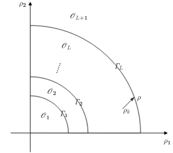
ΛL(ρ)=4i=1nρi2πnLi=1nj=1naijρi2πnLρj2πnL.\Lambda_{L}(\rho)=4\sum_{i=1}^{n}\frac{\rho_{i}}{2\pi n_{L}}-\sum_{i=1}^{n}\sum_{j=1}^{n}a_{ij}\frac{\rho_{i}}{2\pi n_{L}}\frac{\rho_{j}}{2\pi n_{L}}.
Refer to caption
Figure 1. Example of profile of bubbling solutions

We use 𝒪L\mathcal{O}_{L} to denote the region between ΓL1\Gamma_{L-1} and ΓL\Gamma_{L}, the main purpose of this article is to study the profile of bubbling solutions uku^{k} when ρk=(ρ1k,,ρnk)ρ=(ρ1,..,ρn)ΓL\rho^{k}=(\rho_{1}^{k},...,\rho_{n}^{k})\to\rho=(\rho_{1},..,\rho_{n})\in\Gamma_{L}. Here ρΓL\rho\in\Gamma_{L} (L1L\geq 1) is a limit point, ρk=(ρ1k,..,ρnk)\rho^{k}=(\rho_{1}^{k},..,\rho_{n}^{k}) is a sequence of parameters corresponding to bubbling solutions uk=(u1k,,unk)u^{k}=(u^{k}_{1},...,u^{k}_{n}), which satisfies

(1.4) Δguik+jaijρjk(𝔥jkeujkM𝔥jkeujk1)=0\Delta_{g}u_{i}^{k}+\sum_{j}a_{ij}\rho_{j}^{k}(\frac{\mathfrak{h}_{j}^{k}e^{u_{j}^{k}}}{\int_{M}\mathfrak{h}_{j}^{k}e^{u_{j}^{k}}}-1)=0

where around each ptp_{t} (t=1,,Lt=1,...,L) 𝔥tk=|xpt|2γthtk(x)\mathfrak{h}_{t}^{k}=|x-p_{t}|^{2\gamma_{t}}h_{t}^{k}(x) for some smooth function htk(x)h_{t}^{k}(x) with uniform C3C^{3} bound: There exists c>0c>0 independent of kk such that

(1.5) 1chtk(x)c,htk(x)C3c.\frac{1}{c}\leq h_{t}^{k}(x)\leq c,\quad\|h_{t}^{k}(x)\|_{C^{3}}\leq c.

The aim of this article is to provide a complete and precise blowup analysis for ρkρ\rho^{k}\to\rho as kk\to\infty. The information we shall provide includes comparison of bubbling heights, difference between energy integration around blowup points, leading term of ρkρ\rho^{k}-\rho, location of regular blowup points and new relation on coefficient functions around different blowup points. First we observe that the normal vector at ρ\rho is proportional to

(j=1na1jρj2πnL2,,j=1nanjρj2πnL2).(\sum_{j=1}^{n}a_{1j}\frac{\rho_{j}}{2\pi n_{L}}-2,\cdots,\sum_{j=1}^{n}a_{nj}\frac{\rho_{j}}{2\pi n_{L}}-2).

Based on our previous work [27] all these components are positive. For convenience we set

(1.6) 𝔪i=j=1naijρj2πnL,𝔪=mini{𝔪i},\mathfrak{m}_{i}=\sum_{j=1}^{n}a_{ij}\frac{\rho_{j}}{2\pi n_{L}},\quad\mathfrak{m}=\min_{i}\{\mathfrak{m}_{i}\},

and we assume a controlled behavior of ρkρ\rho^{k}\to\rho:

(1.7) ρikρiρjkρj1ijI:={1,,n}.\frac{\rho_{i}^{k}-\rho_{i}}{\rho_{j}^{k}-\rho_{j}}\sim 1\quad\forall\quad i\neq j\in I:=\{1,...,n\}.

Note that AkBkA_{k}\sim B_{k} means CAkBkC1AkCA_{k}\leq B_{k}\leq C_{1}A_{k} for some C,C1>0C,C_{1}>0 independent of kk. We say ρk\rho^{k} tends to ΓL\Gamma_{L} non-tangentially if (1.7) holds.

When ρkρΓL\rho^{k}\to\rho\in\Gamma_{L}, if blowup occurs, let p1p_{1},…,pL2p_{L_{2}} be blowup points, since singular sources may also be blowup points, we use p1.,,,pL1p_{1}.,,,p_{L_{1}} to denote regular blowup points and pL1+1,pL2p_{L_{1}+1}...,p_{L_{2}} to denote singular blowup points. It is proved (see [44, 27]) that they satisfy

(1.8) i=1n((loghi)(pt)+2πms=1L2μs1G(pt,ps))ρi=0,t=1,..,L1.\sum_{i=1}^{n}\bigg{(}\nabla(\log h_{i})(p_{t})+2\pi\mathrm{m}\sum_{s=1}^{L_{2}}\mu_{s}\nabla_{1}G^{*}(p_{t},p_{s})\bigg{)}\rho_{i}=0,\quad t=1,..,L_{1}.

where μs=1+γs\mu_{s}=1+\gamma_{s} (so μs=1\mu_{s}=1 if psp_{s} is a regular point),

(1.9) G(ptk,psk)={γ(ptk,ptk),s=t,G(ptk,psk),st.s,t=1,,N.G^{*}(p_{t}^{k},p_{s}^{k})=\left\{\begin{array}[]{ll}\gamma(p_{t}^{k},p_{t}^{k}),\quad s=t,\\ G(p_{t}^{k},p_{s}^{k}),\quad s\neq t.\end{array}\right.\qquad s,t=1,...,N.

Thus (p1,,pL1)(p_{1},...,p_{L_{1}}) is a critical point of the following function:

(1.10) f(x1,xL1)=t=1L1(i=1nρiloghi(xt))+(i=1nρi)π𝔪t,s=1L1G(xt,xs)\displaystyle f(x_{1},...x_{L_{1}})=\sum_{t=1}^{L_{1}}(\sum_{i=1}^{n}\rho_{i}\log h_{i}(x_{t}))+(\sum_{i=1}^{n}\rho_{i})\pi\mathfrak{m}\sum_{t,s=1}^{L_{1}}G^{*}(x_{t},x_{s})
+(i=1nρi)2π𝔪t=1L1s=L1+1L2G(xt,ps).\displaystyle+(\sum_{i=1}^{n}\rho_{i})2\pi\mathfrak{m}\sum_{t=1}^{L_{1}}\sum_{s=L_{1}+1}^{L_{2}}G^{*}(x_{t},p_{s}).

Thus if det(D2f)det(D^{2}f) is not zero at each critical point, the critical points are disjoint. As a consequence of the blowup analysis we shall carry out in this work, we present our main theorem as follows:

Theorem 1.1.

Let p1,pL1,pL1+1,..,pL2p_{1},...p_{L_{1}},p_{L_{1}+1},..,p_{L_{2}} satisfy (1.8) and D2fD^{2}f be non-degenerate at critical points of ff. Then there exists constants ct>0c_{t}^{*}>0 such that if

(1.11) Δ(loghik)(pt)2K(ptk)+2πnLct for all pt,t=1,,L1,\Delta(\log h_{i}^{k})(p_{t})-2K(p_{t}^{k})+2\pi n_{L}\geq c_{t}^{*}\quad\mbox{ for all $p_{t}$},\quad t=1,...,L_{1},

uku^{k} is uniformly bounded as ρk\rho^{k} tends to ΓL\Gamma_{L} from above non-tangentially, where uk=(u1k,,unk)u^{k}=(u_{1}^{k},...,u_{n}^{k}) is a sequence of solutions to (1.4), ctc_{t}^{*} depends only on 𝔪\mathfrak{m}, the distance from ptp_{t} to the nearest other blowup point and the injectivity radius at ptp_{t},

Theorem 1.1 follows naturally from the complete bubble interaction results in the next section. If the system is reduced to a single equation, a rather detailed blowup analysis has been done by many people [2, 3, 4, 5, 16, 17, 18, 19, 29, 38, 39, 52, 53, 54, 55, 58, 59]. For a single Liouville equation, the total energy of all solutions is just one number. However, for Liouville systems defined on 2\mathbb{R}^{2}, it is established in [21, 42] that total energy of all components form a n1n-1 dimensional hyper-surface similar to Γ1\Gamma_{1}. This continuum of energy brings great difficulty to blowup analysis. A simplest description is this: if ρkΓ2\rho^{k}\to\Gamma_{2} and there are two bubbling disks. Around each bubbling disk, the local energy tends to Γ1\Gamma_{1}, but in order to know exactly how ρkΓ2\rho^{k}\to\Gamma_{2} one needs precise information about how the local energy is tending to Γ1\Gamma_{1} and the comparison of bubbling profiles around different blowup points. This seems to be a unique feature of Liouville systems. In 2013 Lin and the second author published an article [44] that describes ρkΓ1\rho^{k}\to\Gamma_{1}, which avoided this major difficulty. So the main contribution in this article is to completely present the details of bubble interactions. To put our key idea in short, we show that first, bubbling solutions are sufficiently close to global solutions in a neighborhood of the blowup points. Since global solutions are radial, their behavior is determined by their initial conditions. In [42] Lin and Zhang established an important one-to-one correspondence between the initial condition and the total integration of Liouville system. It is based on this principle we are able to obtain the precise comparison among profiles at different blowup points. The reason in this article we require all the singular sources to have negative strength is because we have a classification theorem for such Liouville systems [45].

The organization of this article is as follows: In section two we state our results on bubble interactions, which lead to the proof of the main theorem at the end of this section. In section three we write the equation around a local blowup point, which happens to be a singular source. Then in section four we prove the main estimates that the profiles of bubbling solutions are extremely close around different blowup points. As a result of the main estimates of section four we prove Theorem 2.1,Theorem 2.6 and Theorem 2.2. Section five is dedicated to proving the leading terms in Theorem 2.3 and Theorem 2.5. All these results depend on a local estimate proved in section six.

2. Results on bubble interactions

It is established in [43] that when ρk=(ρ1k,..,ρnk)\rho^{k}=(\rho_{1}^{k},..,\rho_{n}^{k}) tends to ρΓL\rho\in\Gamma_{L} non-tangentially, suppose there are L2L_{2} blowup solutions p1,,pNp_{1},...,p_{N}, some of them may be singular sources, some may be regular points. It is proved in [27] that

(2.1) nL=s=1L2μs.n_{L}=\sum_{s=1}^{L_{2}}\mu_{s}.

In [44] Lin-Zhang derived the leading term when there is no singular source and ρk\rho^{k} tends to the first critical hyper-surface ρkΓ1\rho^{k}\to\Gamma_{1}. The main reason they can only discuss ρΓ1\rho\to\Gamma_{1} is because there is only one blowup point in this case. Whether or not the same level of error estimate can still be obtained for multiple-bubble-situations (ρΓN\rho\to\Gamma_{N}) was a major obstacle for Liouville systems in general. Recently Huang-Zhang [30] completely solved this problem by extending Lin-Zhang’s result to ρkΓN\rho^{k}\to\Gamma_{N} for any NN. But Huang-Zhang’s article does not include the singular cases. It is our goal to further extend all the theorems in [30] to singular Liouville systems.

One point on ΓL\Gamma_{L} plays a particular role: Let Q=(Q1,Qn)Q=(Q_{1},...Q_{n}) be defined by jaijQj=8πnL\sum_{j}a_{ij}Q_{j}=8\pi n_{L} for each ii. Our approximating theorems depend on whether ρ=Q\rho=Q or not.

For simplicity we set

(2.2) u^ik(x)=uik(x)logM𝔥ikeuik𝑑Vg,\hat{u}_{i}^{k}(x)=u_{i}^{k}(x)-\log\int_{M}\mathfrak{h}_{i}^{k}e^{u_{i}^{k}}dV_{g},

thus we have

M𝔥iku^ik𝑑Vg=1,\int_{M}\mathfrak{h}_{i}^{k}\hat{u}_{i}^{k}dV_{g}=1,

and

(2.3) Δgu^ik(x)+j=1naijρjk(𝔥jkeu^jk1)=0,iI.\Delta_{g}\hat{u}_{i}^{k}(x)+\sum_{j=1}^{n}a_{ij}\rho_{j}^{k}(\mathfrak{h}_{j}^{k}e^{\hat{u}_{j}^{k}}-1)=0,\quad i\in I.

Let

(2.4) Mk,t=maxiImaxxB(pt,δ0)u^ik(x)μt,M_{k,t}=\max_{i\in I}\max_{x\in B(p_{t},\delta_{0})}\frac{\hat{u}_{i}^{k}(x)}{\mu_{t}},

be the maximum over B(ptk,δ0)B(p_{t}^{k},\delta_{0}) divided by μl\mu_{l}. Here δ0\delta_{0} is small enough so that B(pt1,δ0)B(pt2,δ0)=B(p_{t_{1}},\delta_{0})\cap B(p_{t_{2}},\delta_{0})=\emptyset for all t1t2t_{1}\neq t_{2}, γt=0\gamma_{t}=0 (μt=1\mu_{t}=1) if ptp_{t} is a regular point. Let

(2.5) Mk=maxtMk,t,ϵk=e12Mk.M_{k}=\max_{t}M_{k,t},\quad\epsilon_{k}=e^{-\frac{1}{2}M_{k}}.

One natural question is What is the relation between MtkM_{t}^{k}?. The answer of this question is presented in this theorem:

Theorem 2.1.

Let ukoH1,n(M)u^{k}\in\,\,^{\text{\r{}}}H^{1,n}(M) be a sequence of blowup solutions of (1.4). Suppose (H1)&(H2)(H1)\&(H2) holds for AA, (1.7) holds for ρk\rho^{k} and 𝔥tk\mathfrak{h}_{t}^{k} is described by (1.5). Then

(2.6) |μsMk,sμtMk,t|=O(1), for s,t{1,,N}.|\mu_{s}M_{k,s}-\mu_{t}M_{k,t}|=O(1),\quad\text{ for }\,\,s,t\in\{1,\cdots,N\}.
Remark 2.1.

Theorem 2.1 implies that μtMk,tMk=O(1)\mu_{t}M_{k,t}-M_{k}=O(1) for all tt.

It is proved in [27] that MtB(pt,δ0)𝔥ikeu^ik=o(1)\displaystyle{\int_{M\setminus\cup_{t}B(p_{t},\delta_{0})}\mathfrak{h}_{i}^{k}e^{\hat{u}_{i}^{k}}=o(1)}. Moreover for any two blowup points p,qp,q,

limkB(p,δ)𝔥ikeu^ikμp=limkB(q,δ)𝔥ikeu^ikμq,\frac{\lim_{k\to\infty}\int_{B(p,\delta)}\mathfrak{h}_{i}^{k}e^{\hat{u}_{i}^{k}}}{\mu_{p}}=\frac{\lim_{k\to\infty}\int_{B(q,\delta)}\mathfrak{h}_{i}^{k}e^{\hat{u}_{i}^{k}}}{\mu_{q}},

where δ>0\delta>0 is small to make bubbling disks mutually disjoint. The second main question is What is the exact difference between them?

Our next result is

Theorem 2.2.

Under the same assumptions in Theorem 2.1.

  • (1)

    Let ρkρΓL\rho^{k}\to\rho\in\Gamma_{L} from 𝒪L\mathcal{O}_{L} or 𝒪L+1\mathcal{O}_{L+1} as in (1.7). If ρQ\rho\neq Q or ρ=Q\rho=Q but there is no regular blowup point, then for any sts\neq t,

    (2.7) |B(p,δ)𝔥ikeu^ikμpB(q,δ)𝔥ikeu^ikμq|=O(ϵk𝔪2),|\frac{\int_{B(p,\delta)}\mathfrak{h}_{i}^{k}e^{\hat{u}_{i}^{k}}}{\mu_{p}}-\frac{\int_{B(q,\delta)}\mathfrak{h}_{i}^{k}e^{\hat{u}_{i}^{k}}}{\mu_{q}}|=O(\epsilon_{k}^{\mathfrak{m}-2}),

    for iIi\in I and ϵk=eMk/2\epsilon_{k}=e^{-M_{k}/2}, 𝔪\mathfrak{m} is defined in (1.6).

  • (2)

    Let ρkQ\rho^{k}\to Q from 𝒪L\mathcal{O}_{L} or 𝒪L+1\mathcal{O}_{L+1}, if there is at least one regular blowup point, then

    (2.8) |B(p,δ)𝔥ikeu^ikμpB(q,δ)𝔥ikeu^ikμq|=O(ϵk2log1ϵk).|\frac{\int_{B(p,\delta)}\mathfrak{h}_{i}^{k}e^{\hat{u}_{i}^{k}}}{\mu_{p}}-\frac{\int_{B(q,\delta)}\mathfrak{h}_{i}^{k}e^{\hat{u}_{i}^{k}}}{\mu_{q}}|=O(\epsilon_{k}^{2}\log\frac{1}{\epsilon_{k}}).
Remark 2.2.

Theorem 2.2 represents the major difficulty in blowup analysis for Liouville systems. Since the mass of a system satisfies a n1n-1 dimensional hypersurface, it is particularly difficult to obtain a precise estimate on the profile of bubbling solutions around different blowup point. Theorem 2.2 is a complete resolution of this long standing difficulty.

Then we define L2L_{2} open sets Ωt,δ1\Omega_{t,\delta_{1}} such that they are mutually disjoint, each of them contains a bubbling disk and their union is MM:

(2.9) B(ptk,δ1)Ωt,δ1,t=1L2Ωt,δ1¯=M,Ωt,δ1Ωs,δ1=,ts.B(p_{t}^{k},\delta_{1})\subset\Omega_{t,\delta_{1}},\quad\cup_{t=1}^{L_{2}}\overline{\Omega_{t,\delta_{1}}}=M,\quad\Omega_{t,\delta_{1}}\cap\Omega_{s,\delta_{1}}=\emptyset,\,\,\forall t\neq s.

Next we set

(2.10) Ai,t,δ\displaystyle A_{i,t,\delta}
=\displaystyle= δμt(2𝔪)μt𝔪22πΩ^t,δ|xpt|2γthik(x)hik(ptk)e2π𝔪l=1L2μl(G(x,plk)G(ptk,plk))𝑑Vg\displaystyle\frac{\delta^{\mu_{t}(2-\mathfrak{m})}}{\mu_{t}}-\frac{\mathfrak{m}-2}{2\pi}\int_{\hat{\Omega}_{t,\delta}}|x-p_{t}|^{2\gamma_{t}}\frac{h_{i}^{k}(x)}{h_{i}^{k}(p_{t}^{k})}e^{2\pi\mathfrak{m}\sum_{l=1}^{L_{2}}\mu_{l}(G(x,p_{l}^{k})-G^{*}(p_{t}^{k},p_{l}^{k}))}dV_{g}

where Ω^t,δ=Ωt,δ1B(ptk,δ)\hat{\Omega}_{t,\delta}=\Omega_{t,\delta_{1}}\setminus B(p_{t}^{k},\delta). Then for fixed kk limδ0Ai,δ\lim_{\delta\to 0}A_{i,\delta} exists because the leading term from the Green’s function is 12πlog|xptk|-\frac{1}{2\pi}\log|x-p_{t}^{k}|. In the next two theorems we identify the leading terms.

Theorem 2.3.

Suppose the same assumptions in Theorem 2.1 hold and let ρkρΓL\rho^{k}\to\rho\in\Gamma_{L} from 𝒪L\mathcal{O}_{L} or 𝒪L+1\mathcal{O}_{L+1} non-tangentially. If either ρQ\rho\neq Q or ρ=Q\rho=Q but there is no regular blowup point, then

(2.11) ΛL(ρk)=(D+o(1))ϵk𝔪2nL.\Lambda_{L}(\rho^{k})=(D+o(1))\frac{\epsilon_{k}^{\mathfrak{m}-2}}{n_{L}}.

where DD is defined as

D=iI1t=1L2Bitlimδ0Ai,t,δ,D=\sum_{i\in I_{1}}\sum_{t=1}^{L_{2}}B_{it}\lim_{\delta\to 0}A_{i,t,\delta},

for Ai,t,δA_{i,t,\delta} in (2.10) and I1:={iI;𝔪i=𝔪}I_{1}:=\{i\in I;\quad\mathfrak{m}_{i}=\mathfrak{m}\}, o(1)0o(1)\to 0 as δ0\delta\to 0, Ω^t,δ0=Ωt,δB(ptk,δ)\hat{\Omega}_{t,\delta_{0}}=\Omega_{t,\delta}\setminus B(p_{t}^{k},\delta), and

Bit=e2π𝔪l=1L2μlG(ptk,plk)e2π𝔪l=1L2μlG(p1k,plk)hik(ptk)hik(p1k)eDiαiB_{it}=\frac{e^{2\pi\mathfrak{m}\sum_{l=1}^{L_{2}}\mu_{l}G^{*}(p_{t}^{k},p_{l}^{k})}}{e^{2\pi\mathfrak{m}\sum_{l=1}^{L_{2}}\mu_{l}G^{*}(p_{1}^{k},p_{l}^{k})}}\frac{h_{i}^{k}(p_{t}^{k})}{h_{i}^{k}(p_{1}^{k})}e^{D_{i}-\alpha_{i}}

and DiD_{i}, αi\alpha_{i} are constants determined by the limit of uku^{k} after scaling ( see (4.22)).

It can be observed that if ρk\rho^{k} tends to ΓL\Gamma_{L} from 𝒪L\mathcal{O}_{L} (that is, tending to ΓL\Gamma_{L} from inside), ΛL(ρk)>0\Lambda_{L}(\rho^{k})>0 for ρk𝒪L\rho^{k}\in\mathcal{O}_{L} and ΛL(ρk)<0\Lambda_{L}(\rho^{k})<0 for ρk𝒪L+1\rho^{k}\in\mathcal{O}_{L+1}. Thus, if D0D\not=0, the blowup solutions with ρk\rho^{k} occur as ρkρΓL\rho^{k}\to\rho\in\Gamma_{L} only from one side of ΓL\Gamma_{L}. Furthermore, it yields a uniform bound of solutions as ρk\rho^{k} converges to ΓL(ρQ)\Gamma_{L}(\rho\not=Q) from 𝒪L\mathcal{O}_{L} provided that D<0D<0. The study of the sign of DD is another interesting fundamental question. Besides consideration on the compactness of solutions, the sign of DD is important for constructing blowup solutions with critical parameters and the uniqueness of bubbling solutions. These projects will be carried out in a different work.

The next result is concerned with the leading term of ΛL(ρk)\Lambda_{L}(\rho^{k}) when ρkQ\rho^{k}\to Q:

Theorem 2.4.

Under the same assumptions in Theorem 2.1. If ρkQ\rho^{k}\to Q from 𝒪L\mathcal{O}_{L} or 𝒪L+1\mathcal{O}_{L+1} non-tangentially, and there is at least one regular blowup point, then

(2.12) ΛL(ρk)=4i=1nt=1L1bitkϵk2logϵk1+O(ϵk2),\Lambda_{L}(\rho^{k})=-4\sum_{i=1}^{n}\sum_{t=1}^{L_{1}}b_{it}^{k}\epsilon_{k}^{2}\log\epsilon_{k}^{-1}+O(\epsilon_{k}^{2}),

where

bitk\displaystyle b_{it}^{k} =eDiαi(14Δ(loghik)(ptk)K(ptk)2+2πNL\displaystyle=e^{D_{i}-\alpha_{i}}\bigg{(}\frac{1}{4}\Delta(\log h_{i}^{k})(p_{t}^{k})-\frac{K(p_{t}^{k})}{2}+2\pi N_{L}
+14|(loghik)(ptk)+8πl=1L21G(ptk,plk)|2)\displaystyle+\frac{1}{4}|\nabla(\log h_{i}^{k})(p_{t}^{k})+8\pi\sum_{l=1}^{L_{2}}\nabla_{1}G^{*}(p_{t}^{k},p_{l}^{k})|^{2}\bigg{)}

and KK is the Gaussian curvature.

Remark 2.3.

The leading term in Theorem 2.3 is involved with integration on the whole MM, but the leading term in Theorem 2.4 only depends on the information at regular blowup points.

The fifth result is about the locations of the regular blowup points:

Theorem 2.5.

If ρkρQ\rho^{k}\to\rho\neq Q as in (1.7), then for each regular blowup point ptp_{t} (t=1,,L1t=1,...,L_{1})

(2.13) i=1n((loghik)(ptk)+2π𝔪s=1Nμs1G(ptk,psk))ρi=O(ϵk𝔪2)\sum_{i=1}^{n}\bigg{(}\nabla(\log h_{i}^{k})(p_{t}^{k})+2\pi\mathfrak{m}\sum_{s=1}^{N}\mu_{s}\nabla_{1}G^{*}(p_{t}^{k},p_{s}^{k})\bigg{)}\rho_{i}=O(\epsilon_{k}^{\mathfrak{m}-2})

where 1\nabla_{1} means the differentiation with respect to the first component. If ρkQ\rho^{k}\to Q as in (1.7),

(2.14) i=1n((loghik)(ptk)+8πs=1L2μs1G(ptk,psk))qi=O(ϵk2logϵk1),\sum_{i=1}^{n}\bigg{(}\nabla(\log h_{i}^{k})(p_{t}^{k})+8\pi\sum_{s=1}^{L_{2}}\mu_{s}\nabla_{1}G^{*}(p_{t}^{k},p_{s}^{k})\bigg{)}q_{i}=O(\epsilon_{k}^{2}\log\epsilon_{k}^{-1}),

for each regular blowup point ptp_{t}.

The sixth main result is a surprising restriction on coefficient function hikh_{i}^{k}.

Theorem 2.6.

Let

Hit=2π𝔪i𝔪i2(l=1L2μlG(ptk,plk))+1𝔪i2loghik(ptk)μt𝔪iH_{it}=\frac{2\pi\mathfrak{m}_{i}}{\mathfrak{m}_{i}-2}(\sum_{l=1}^{L_{2}}\mu_{l}G^{*}(p_{t}^{k},p_{l}^{k}))+\frac{1}{\mathfrak{m}_{i}-2}\log\frac{h_{i}^{k}(p_{t}^{k})}{\mu_{t}^{\mathfrak{m}_{i}}}

where 𝔪i=j=1naijρj2πnL\mathfrak{m}_{i}=\sum_{j=1}^{n}a_{ij}\frac{\rho_{j}}{2\pi n_{L}}. Then

HitHis=HjtHjs+E,i,j=1,,n,t,s=1,,L2.H_{it}-H_{is}=H_{jt}-H_{js}+E,\quad\forall i,j=1,...,n,\quad t,s=1,...,L_{2}.

Obviously Theorem 2.6 is not seen in the case of L2=1L_{2}=1 and reveals new relations on coefficient functions hikh_{i}^{k}. In other words, if one constructs bubbling solutions, the hikh_{i}^{k}s need to satisfy the statement of Theorem 2.6, in addition to other key information such as precise information about bubbling interactions, exact location of blowup points, accurate vanishing rate of coefficient functions and specific leading terms in asymptotic expansions. All these have been covered in the main results of this article. The construction of bubbling solutions will be carried out in other works in the future.

2.1. Proof of Theorem 1.1

Finally in this section we provide the proof of Theorem 1.1. We consider two cases. In the first when the the limit point ρQ\rho\neq Q, the blowup analysis gives 𝔪<4\mathfrak{m}<4. The second case if when ρ=Q\rho=Q and 𝔪=4\mathfrak{m}=4 in this case.

When ρQ\rho\neq Q we prove that Ai,t,δ0A_{i,t,\delta}\leq 0 for each tt under the curvature assumption. From the definition of Ai,t,δA_{i,t,\delta} we have

Ai,t,δδμt(2𝔪)μt𝔪22π𝔅ϵ0|xpt|2γthi(x)hik(pt)e2π𝔪l=1L2μl(G(x,plk)G(ptk,plk))𝑑VgA_{i,t,\delta}\leq\frac{\delta^{\mu_{t}(2-\mathfrak{m})}}{\mu_{t}}-\frac{\mathfrak{m}-2}{2\pi}\int_{\mathfrak{B}_{\epsilon_{0}}}|x-p_{t}|^{2\gamma_{t}}\frac{h_{i}(x)}{h_{i}^{k}(p_{t})}e^{2\pi\mathfrak{m}\sum_{l=1}^{L_{2}}\mu_{l}(G(x,p_{l}^{k})-G^{*}(p_{t}^{k},p_{l}^{k}))}dV_{g}

where 𝔅ϵ0=B(pt,ϵ0)B(pt,δ)\mathfrak{B}_{\epsilon_{0}}=B(p_{t},\epsilon_{0})\setminus B(p_{t},\delta). When we evaluate the integration on 𝔅ϵ0\mathfrak{B}_{\epsilon_{0}} we use dVg=eϕdxdV_{g}=e^{\phi}dx to obtain

𝔪22π𝔅ϵ0|xpt|2γthi(x)hik(pt)e2π𝔪l=1L2μl(G(x,plk)G(ptk,plk))𝑑Vg\displaystyle-\frac{\mathfrak{m}-2}{2\pi}\int_{\mathfrak{B}_{\epsilon_{0}}}|x-p_{t}|^{2\gamma_{t}}\frac{h_{i}(x)}{h_{i}^{k}(p_{t})}e^{2\pi\mathfrak{m}\sum_{l=1}^{L_{2}}\mu_{l}(G(x,p_{l}^{k})-G^{*}(p_{t}^{k},p_{l}^{k}))}dV_{g}
ϵ0μt(2𝔪)μtδμt(2𝔪)μt\displaystyle\leq\frac{\epsilon_{0}^{\mu_{t}(2-\mathfrak{m})}}{\mu_{t}}-\frac{\delta^{\mu_{t}(2-\mathfrak{m})}}{\mu_{t}}
(𝔪2)(ϵ02(𝔪2)μtδ2(𝔪2)μt)4(2(𝔪2)μt)(Δ(loghi)(pt)2K(pt)+2πnl)\displaystyle-\frac{(\mathfrak{m}-2)(\epsilon_{0}^{2-(\mathfrak{m}-2)\mu_{t}}-\delta^{2-(\mathfrak{m}-2)\mu_{t}})}{4(2-(\mathfrak{m}-2)\mu_{t})}(\Delta(\log h_{i})(p_{t})-2K(p_{t})+2\pi n_{l})

Note that the reason we have an inequality is because we drop the square of the first derivatives in the exponential function, which is positive. Thus, as long as

Δ(loghi)(pt)2K(pt)+2πnl>4(2(𝔪2)μt)(𝔪2)μtϵ02,t,\Delta(\log h_{i})(p_{t})-2K(p_{t})+2\pi n_{l}>\frac{4(2-(\mathfrak{m}-2)\mu_{t})}{(\mathfrak{m}-2)\mu_{t}}\epsilon_{0}^{-2},\quad\forall t,

ΛL(ρk)\Lambda_{L}(\rho^{k}) is negative, so if ρk\rho^{k} is tending to ρ\rho from above non-tangentially, the blow-up does not happen. The existence of ϵ0\epsilon_{0} depends on the injectivity radius, the distance from ptkp_{t}^{k} to other blowup point and singularities. The argument for ρkQ\rho^{k}\to Q is similar. Theorem 1.1 is established. \Box

3. The profile of bubbling solutions around a singular source

In this section we write the equation (1.4) around a singular source pp, which is also a blowup point. Suppose that the strength of the singularity is 4πγp4\pi\gamma_{p} with γp(1,0)\gamma_{p}\in(-1,0), we derive an approximation theorem for blow-up solutions uku^{k} around pp. To state more precise approximation results we write the equation in local coordinate around pp. In this coordinate, ds2ds^{2} has the form

eϕ(yp)[(dy1)2+(dy2)2],e^{\phi(y_{p)}}[(dy^{1})^{2}+(dy^{2})^{2}],

where

ϕ(0)=0,ϕ(0)=0.\nabla\phi(0)=0,\phi(0)=0.

Also near pp we have

Δypϕ=2Keϕ,whereKistheGausscurvature.\Delta_{y_{p}}\phi=-2Ke^{\phi},\quad{\rm where}\hskip 2.84544ptK{\rm\hskip 2.84544ptis\hskip 2.84544ptthe\hskip 2.84544ptGauss\hskip 2.84544ptcurvature}.

Here we invoke a result proved in our previous work [27] since γp\gamma_{p} is not a positive integer, the spherical Harnack inequality holds around pp and pp is the only blowup point in B(p,δ)B(p,\delta). Here we recall that in a neighborhood of pp, 𝔥ik(x)=|x|2γphik(x)\mathfrak{h}_{i}^{k}(x)=|x|^{2\gamma_{p}}h_{i}^{k}(x).

In this local coordinates, (1.4) is of the form

(3.1) Δuik=j=1naijρjkeϕ(|x|2γphjkeujkM𝔥jkeujk1),B(0,δ).-\Delta u_{i}^{k}=\sum_{j=1}^{n}a_{ij}\rho_{j}^{k}e^{\phi}(\frac{|x|^{2\gamma_{p}}h_{j}^{k}e^{u_{j}^{k}}}{\int_{M}\mathfrak{h}^{k}_{j}e^{u_{j}^{k}}}-1),\hskip 5.69046ptB(0,\delta).

Going back to (3.1), we let fikf_{i}^{k} be defined as

Δfik=j=1naijρjkeϕ,inB(0,δ),andfik(0)=|fik(0)|=0.\Delta f_{i}^{k}=\sum_{j=1}^{n}a_{ij}\rho_{j}^{k}e^{\phi},\quad{\rm in}\hskip 2.84544ptB(0,\delta),\quad\mbox{and}\quad f_{i}^{k}(0)=|\nabla f_{i}^{k}(0)|=0.

Then we have

Δ(u^ikfik)+j=1naijρjk|x|2γphjkeu^jkfjkefjkeϕ=0,inB(0,δ),\Delta(\hat{u}_{i}^{k}-f_{i}^{k})+\sum_{j=1}^{n}a_{ij}\rho_{j}^{k}|x|^{2\gamma_{p}}h_{j}^{k}e^{\hat{u}_{j}^{k}-f_{j}^{k}}e^{f_{j}^{k}}e^{\phi}=0,\quad{\rm in}\hskip 2.84544ptB(0,\delta),

which can be further written as

(3.2) Δu~ik+j=1naij|x|2γph~jkeu~jk=0,B(0,δ).\Delta\tilde{u}_{i}^{k}+\sum_{j=1}^{n}a_{ij}|x|^{2\gamma_{p}}\tilde{h}_{j}^{k}e^{\tilde{u}_{j}^{k}}=0,\hskip 5.69046ptB(0,\delta).

if we set

h~ik(x)=hik(x)hik(p)eϕ+fik,which impliesh~ik(0)=1,\tilde{h}_{i}^{k}(x)=\frac{h_{i}^{k}(x)}{h_{i}^{k}(p)}e^{\phi+f_{i}^{k}},\quad\mbox{which implies}\quad\tilde{h}_{i}^{k}(0)=1,

and

(3.3) u~ik=u^ik+log(ρikhik(p))fik,\tilde{u}_{i}^{k}=\hat{u}_{i}^{k}+\log(\rho_{i}^{k}h_{i}^{k}(p))-f_{i}^{k},

Now we introduce ϕik\phi_{i}^{k} to be a harmonic function defined by the oscillation of u~ik\tilde{u}_{i}^{k} on B(p,δ)B(p,\delta):

(3.4) {Δϕik=0,inB(0,δ),ϕik=u~ik12πδB(0,δ)u~ik,onB(0,δ)\left\{\begin{array}[]{ll}-\Delta\phi_{i}^{k}=0,\quad{\rm in}\hskip 2.84544ptB(0,\delta),\\ \phi_{i}^{k}=\tilde{u}_{i}^{k}-\frac{1}{2\pi\delta}\int_{\partial B(0,\delta)}\tilde{u}_{i}^{k},\quad{\rm on}\hskip 2.84544pt\partial B(0,\delta)\end{array}\right.

Obviously, ϕik(0)=0\phi_{i}^{k}(0)=0 by the mean value theorem and ϕik\phi_{i}^{k} is uniformly bounded on B(0,δ/2)B(0,\delta/2) because uiku_{i}^{k} has finite oscillation away from blowup points. Now we set

(3.5) Mk,p=maxiIu~ik(p)μp,εk,p=eMk,p2,μp=1+γpM_{k,p}=\frac{\max_{i\in I}\tilde{u}_{i}^{k}(p)}{\mu_{p}},\quad\varepsilon_{k,p}=e^{-\frac{M_{k,p}}{2}},\quad\mu_{p}=1+\gamma_{p}

and

σipk=12πB(p,δ)|xpk|2γph~ikeu~ik,mipk=j=1naijσipk,mpk=miniImipk.\sigma_{ip}^{k}=\frac{1}{2\pi}\int_{B(p,\delta)}|x-p_{k}|^{2\gamma_{p}}\tilde{h}_{i}^{k}e^{\tilde{u}_{i}^{k}},\quad m_{ip}^{k}=\sum_{j=1}^{n}a_{ij}\sigma_{ip}^{k},\quad m_{p}^{k}=\min_{i\in I}m_{ip}^{k}.

It is proved in [27] that

vik(y)=u~ik(p+ϵk,py)+2(1+γp)logϵk,p,|y|<δϵk,p1v_{i}^{k}(y)=\tilde{u}_{i}^{k}(p+\epsilon_{k,p}y)+2(1+\gamma_{p})\log\epsilon_{k,p},\quad|y|<\delta\epsilon_{k,p}^{-1}

converges uniformly to U=(U1,.,Un)U=(U_{1},....,U_{n}) over any fixed compact subset of 2\mathbb{R}^{2} and vv satisfies

(3.6) ΔUi+jaij|y|2γpeUj=0,in2,i=1,..,n.\Delta U_{i}+\sum_{j}a_{ij}|y|^{2\gamma_{p}}e^{U_{j}}=0,\quad\mbox{in}\quad\mathbb{R}^{2},\quad i=1,..,n.

In other words, after the scaling, no component is lost in the limit. We have a fully bubbling sequence. It is also established in [27] that pp is the only blowup point in a neighborhood of pp and uku^{k} satisfies spherical Harnack inequality around pp.

Let Uk=(U1k,,Unk)U^{k}=(U_{1}^{k},\cdots,U_{n}^{k}) be the radial solutions of

(3.7) {ΔUik=j=inaij|x|2γpeUjk,inR2,Uik(0)=vik(0),iI.\left\{\begin{array}[]{ll}-\Delta U_{i}^{k}=\sum_{j=i}^{n}a_{ij}|x|^{2\gamma_{p}}e^{U_{j}^{k}},\quad{\rm in}\hskip 2.84544ptR^{2},\\ U_{i}^{k}(0)=v_{i}^{k}(0),\quad i\in I.\end{array}\right.

This family of global solutions UkU^{k} will be used as the first term in the approximation of vkv^{k}.

Based on Theorem 6.2 we have the following estimate of vikUikv_{i}^{k}-U_{i}^{k}: For multi-index α\alpha (|α|=0|\alpha|=0 or 11)

|Dα(vik(y)Uik(y)ϕik(ϵky)Φik(y)|\displaystyle|D^{\alpha}(v_{i}^{k}(y)-U_{i}^{k}(y)-\phi_{i}^{k}(\epsilon_{k}y)-\Phi_{i}^{k}(y)|
\displaystyle\leq Cϵk,p2(1+|y|)2+2μpmp|α|+ϵ|y|τϵk,p1\displaystyle C\epsilon_{k,p}^{2}(1+|y|)^{2+2\mu_{p}-m_{p}-|\alpha|+\epsilon}\quad|y|\leq\tau\epsilon_{k,p}^{-1}

where ϕik\phi_{i}^{k} is defined in (3.4), C>0C>0 is also independent of kk, mp=limkmpkm_{p}=\lim_{k\to\infty}m_{p}^{k},

Φik(y)=ϵk,p(G1,ik(r)cosθ+G2,ik(r)sinθ),\Phi_{i}^{k}(y)=\epsilon_{k,p}(G_{1,i}^{k}(r)\cos\theta+G_{2,i}^{k}(r)\sin\theta),

with

|Gt,ik(r)|Cr(1+r)2μpmp+ϵ|G_{t,i}^{k}(r)|\leq Cr(1+r)^{2\mu_{p}-m_{p}+\epsilon}

where ϵ>0\epsilon>0 is a small positive constant.

4. The comparison of bubbling profiles

For simplicity we first assume there are only two blowup points pp and qq. The conclusion for the more general situation will be stated at the end of this section. If pp is a singular source, we set Mk,pM_{k,p} be defined as in (3.5). If pp is a regular point, we set

Mk,p=maxxB(p,δ)maxiu~ik(x),M_{k,p}=\max_{x\in B(p,\delta)}\max_{i}\tilde{u}_{i}^{k}(x),

for some small δ>0\delta>0. Mk,qM_{k,q} is understood in the same fashion. Here we require that at least one of p,qp,q is a singular source because the comparison of bubbling profiles for regular blowup points have been done in [30]. Now we use Green’s representation to describe the neighborhood of pp. By (2.3) u^ik\hat{u}_{i}^{k} is

u^ik(x)\displaystyle\hat{u}_{i}^{k}(x) =u¯ik+MG(x,η)j=1naijρjk𝔥jkeu^jkdVg\displaystyle=\bar{u}_{i}^{k}+\int_{M}G(x,\eta)\sum_{j=1}^{n}a_{ij}\rho_{j}^{k}\mathfrak{h}_{j}^{k}e^{\hat{u}_{j}^{k}}dV_{g}
=u¯ik+(B(p,δ)+B(qk,δ)+MB(p,δ))G(x,η)j=1naijρjk𝔥jkeu^jk\displaystyle=\bar{u}_{i}^{k}+\left(\int_{B(p,\delta)}+\int_{B(q_{k},\delta)}+\int_{M\setminus B(p,\delta)}\right)G(x,\eta)\sum_{j=1}^{n}a_{ij}\rho_{j}^{k}\mathfrak{h}_{j}^{k}e^{\hat{u}_{j}^{k}}
=u¯ik+I+II+III.\displaystyle=\bar{u}_{i}^{k}+I+II+III.

Here

u¯ik=Mu^ik𝑑Vg,E=O(ϵkτ)\bar{u}_{i}^{k}=\int_{M}\hat{u}_{i}^{k}dV_{g},\quad E=O(\epsilon_{k}^{\tau})

for some τ>0\tau>0. Note that it is already established in our previous work [27] that (μpMk,p)/(μqMk,q)1(\mu_{p}M_{k,p})/(\mu_{q}M_{k,q})\to 1 as kk\to\infty, the error term around pp in local approximation and computation of Pohozaev identity is O(ϵk,pmk,p2μp)O(\epsilon_{k,p}^{m_{k,p}-2\mu_{p}}) and the error around qq is the similar expression with qq replacing pp and with a possible correction of a logarithmic term. Right now we are using crude bound for the error EE. This bound will be improved later.

For simplicity we use

mik=j=1naijσjk,σik=12πB(pk,δ)ρikhik|η|2γpeu^ik𝑑Vgm_{i}^{k}=\sum_{j=1}^{n}a_{ij}\sigma_{j}^{k},\quad\sigma_{i}^{k}=\frac{1}{2\pi}\int_{B(p_{k},\delta)}\rho_{i}^{k}h_{i}^{k}|\eta|^{2\gamma_{p}}e^{\hat{u}_{i}^{k}}dV_{g}

and m¯ik,σ¯ik\bar{m}_{i}^{k},\bar{\sigma}_{i}^{k} are the integration in B(qk,δ)B(q_{k},\delta). Also we use mkm_{k} to denote the smallest mikm_{i}^{k} and m¯k\bar{m}_{k} is the smallest m¯ik\bar{m}_{i}^{k}. Using Theorem 6.2 to evaluate integrals we have

I\displaystyle I =Bδ(12πlog|η|+ν(x,η))jIaij|η|2γh~jkeu~jkdη\displaystyle=\int_{B_{\delta}}(-\frac{1}{2\pi}\log|\eta|+\nu(x,\eta))\sum_{j\in I}a_{ij}|\eta|^{2\gamma}\tilde{h}_{j}^{k}e^{\tilde{u}_{j}^{k}}d\eta
=miklog|x|+2πmikν(x,pk)+E\displaystyle=-m_{i}^{k}\log|x|+2\pi m_{i}^{k}\nu(x,p_{k})+E
II\displaystyle II =2πm¯ikG(x,qk)+E,III=E\displaystyle=2\pi\bar{m}_{i}^{k}G(x,q_{k})+E,\quad III=E

Thus in the neighborhood of pp,

(4.1) u^ik(x)=u¯ikmiklog|x|+2πmikν(x,pk)+2πm¯ikG(x,qk)+E\hat{u}_{i}^{k}(x)=\bar{u}_{i}^{k}-m_{i}^{k}\log|x|+2\pi m_{i}^{k}\nu(x,p_{k})+2\pi\bar{m}_{i}^{k}G(x,q_{k})+E

and by Lemma 2.3 of [27], we have

(4.2) u¯ik(x)=mi2μp2Mk,p+O(1).\bar{u}_{i}^{k}(x)=-\frac{m_{i}-2\mu_{p}}{2}M_{k,p}+O(1).

Proof of Theorem 2.1.

From (4.2), we obtain

(4.3) mi2μp2Mk,p=m¯i2μq2Mk,q+O(1).-\frac{m_{i}-2\mu_{p}}{2}M_{k,p}=-\frac{\bar{m}_{i}-2\mu_{q}}{2}M_{k,q}+O(1).

Let

λk=μpMk,pμqMk,q,δik=O(1)Mk,q,\lambda_{k}=\frac{\mu_{p}M_{k,p}}{\mu_{q}M_{k,q}},\quad\delta_{i}^{k}=\frac{O(1)}{M_{k,q}},

we can write (4.1) as

(4.4) mi2μp2μpλk+δik=m¯i2μq2μq.-\frac{m_{i}-2\mu_{p}}{2\mu_{p}}\lambda_{k}+\delta_{i}^{k}=-\frac{\bar{m}_{i}-2\mu_{q}}{2\mu_{q}}.

Since the Pohozaev identity gives

i,jaijσikσjk=4μpiσik+E,\sum_{i,j}a_{ij}\sigma_{i}^{k}\sigma_{j}^{k}=4\mu_{p}\sum_{i}\sigma_{i}^{k}+E,

mk=(m1k,,mnk)m^{k}=(m_{1}^{k},\cdots,m_{n}^{k}) satisfies

(4.5) i,jaij(mik2μp2μp)(mjk2μp2μp)=i,jaij+E.\sum_{i,j}a^{ij}\bigg{(}\frac{m_{i}^{k}-2\mu_{p}}{2\mu_{p}}\bigg{)}\bigg{(}\frac{m_{j}^{k}-2\mu_{p}}{2\mu_{p}}\bigg{)}=\sum_{i,j}a^{ij}+E.

and (4.5) also holds for m¯k=(m¯1k,,m¯nk)\bar{m}^{k}=(\bar{m}_{1}^{k},\cdots,\bar{m}_{n}^{k}). Using (4.4) we have

(4.6) i,jaij(mik2μp)2μpλk+δik)(mjk2μp)2μpλk+δjk)=i,jaij+E.\sum_{i,j}a^{ij}\bigg{(}\frac{m_{i}^{k}-2\mu_{p})}{2\mu_{p}}\lambda_{k}+\delta_{i}^{k}\bigg{)}\bigg{(}\frac{m_{j}^{k}-2\mu_{p})}{2\mu_{p}}\lambda_{k}+\delta_{j}^{k}\bigg{)}=\sum_{i,j}a^{ij}+E.

which can be written as

(4.7) λk2i,jaij(mik2μp2μp)(mjk2μp2μp)\displaystyle\lambda_{k}^{2}\sum_{i,j}a^{ij}\bigg{(}\frac{m_{i}^{k}-2\mu_{p}}{2\mu_{p}}\bigg{)}\bigg{(}\frac{m_{j}^{k}-2\mu_{p}}{2\mu_{p}}\bigg{)}
+2λki,jaij(mik2μp2μp)δjk+i,jaijδikδjk=i,jaij+E.\displaystyle+2\lambda_{k}\sum_{i,j}a^{ij}\bigg{(}\frac{m_{i}^{k}-2\mu_{p}}{2\mu_{p}}\bigg{)}\delta_{j}^{k}+\sum_{i,j}a^{ij}\delta_{i}^{k}\delta_{j}^{k}=\sum_{i,j}a^{ij}+E.

Let

Bk=i,jaij(mi2μp2μp)δjki,jaij,Ck=i,jaijδikδjki,jaijB_{k}=\frac{\sum_{i,j}a^{ij}\bigg{(}\frac{m_{i}-2\mu_{p}}{2\mu_{p}}\bigg{)}\delta_{j}^{k}}{\sum_{i,j}a^{ij}},\quad C_{k}=\frac{\sum_{i,j}a^{ij}\delta_{i}^{k}\delta_{j}^{k}}{\sum_{i,j}a^{ij}}

be the coefficients of the following polynomial for λk\lambda_{k}:

λk2+Bkλk+Ck=1+E.\lambda_{k}^{2}+B_{k}\lambda_{k}+C_{k}=1+E.

Our goal is to obtain an upper bound of |λk1||\lambda_{k}-1|. Here we note that since AA satisfies (H1)(H1) and (H2)(H2), i,jaij0\sum_{i,j}a^{ij}\neq 0. It is obvious that limkλk=1\lim_{k\rightarrow\infty}\lambda_{k}=1. Taking advantage of Ck=O(Mk,q2)C_{k}=O(M_{k,q}^{-2}) and Bk=O(Mk,q1)B_{k}=O(M_{k,q}^{-1}) we have

(4.8) λk=Bk2+Bk24(Ck1)=1+O(Mk,q1).\lambda_{k}=-\frac{B_{k}}{2}+\sqrt{\frac{B_{k}^{2}}{4}-(C_{k}-1)}=1+O(M_{k,q}^{-1}).

This verifies μpMk,pμqMk,q=O(1)\mu_{p}M_{k,p}-\mu_{q}M_{k,q}=O(1). Theorem 2.1 is established. \Box

Remark 4.1.

Since (see [27])

limkmikμp=limkm¯ikμq\lim_{k\to\infty}\frac{m_{i}^{k}}{\mu_{p}}=\lim_{k\to\infty}\frac{\bar{m}_{i}^{k}}{\mu_{q}}

and μpMk,pμqMk,q=O(1)\mu_{p}M_{k,p}-\mu_{q}M_{k,q}=O(1), we have Mk,p=O(log1/ϵk,p)M_{k,p}=O(\log 1/\epsilon_{k,p}), and a more precise description of O(ϵk,pmk2μp)O(\epsilon_{k,p}^{m_{k}-2\mu_{p}}) and O(ϵk,qm¯k2μq)O(\epsilon_{k,q}^{\bar{m}_{k}-2\mu_{q}}):

ϵk,pmk2μp=e12μpMk,p(mk,p/μp2)=O(1)e12μqMk,q(m¯k/μq2)=O(ϵk,qm¯k2μq).\epsilon_{k,p}^{m_{k}-2\mu_{p}}=e^{-\frac{1}{2}\mu_{p}M_{k,p}(m_{k,p}/\mu_{p}-2)}=O(1)e^{-\frac{1}{2}\mu_{q}M_{k,q}(\bar{m}_{k}/\mu_{q}-2)}=O(\epsilon_{k,q}^{\bar{m}_{k}-2\mu_{q}}).

Thus O(εk,pmk2μp)=O(εk,qm¯k2μq)=EO(\varepsilon_{k,p}^{m_{k}-2\mu_{p}})=O(\varepsilon_{k,q}^{\bar{m}_{k}-2\mu_{q}})=E. From now on in this section we use EE to denote O(ϵk,pmk2μp)O(\epsilon_{k,p}^{m_{k}-2\mu_{p}}).

By the definition of u~ik\tilde{u}_{i}^{k} in (3.3) and Theorem 6.2, the value of u~ik\tilde{u}_{i}^{k} away from bubbling disks is

(4.9) u~ik(x)=\displaystyle\tilde{u}_{i}^{k}(x)= u¯ikmiklog|x|+2πmikν(x,pk)+2πm¯ikG(x,qk)\displaystyle\bar{u}_{i}^{k}-m_{i}^{k}\log|x|+2\pi m_{i}^{k}\nu(x,p_{k})+2\pi\bar{m}_{i}^{k}G(x,q_{k})
+log(ρikhik(pk))fik(x)+E\displaystyle+\log(\rho_{i}^{k}h_{i}^{k}(p_{k}))-f_{i}^{k}(x)+E

On the other hand u~ik\tilde{u}_{i}^{k} also has the form

(4.10) u~ik(x)ϕik(x)=Vik(x)+E\tilde{u}_{i}^{k}(x)-\phi_{i}^{k}(x)=V_{i}^{k}(x)+E

where VikV_{i}^{k} is the global radial solution that takes the initial value of u~k\tilde{u}^{k}: Vik(0)=u~ik(pk)V_{i}^{k}(0)=\tilde{u}_{i}^{k}(p_{k}). From this expression we see that ϕik\phi_{i}^{k} denotes the “non-radial part” in the expansion of u~ik\tilde{u}_{i}^{k}. Combining (4.9), (4.10) and using the fact that ϕik(0)=0\phi_{i}^{k}(0)=0, we have,

(4.11) ϕik(x)=\displaystyle\phi_{i}^{k}(x)= 2πmik(ν(x,pk)ν(pk,pk))+2πm¯ik(G(x,qk)G(pk,qk))\displaystyle 2\pi m_{i}^{k}(\nu(x,p_{k})-\nu(p_{k},p_{k}))+2\pi\bar{m}_{i}^{k}(G(x,q_{k})-G(p_{k},q_{k}))
fik(x)+E\displaystyle-f_{i}^{k}(x)+E

So in the local coordinate around pp, u~ik\tilde{u}_{i}^{k} can be rewritten as

(4.12) u~ik(x)\displaystyle\tilde{u}_{i}^{k}(x) =miklog|x|+u¯ik+ϕik(x)\displaystyle=-m_{i}^{k}\log|x|+\bar{u}_{i}^{k}+\phi_{i}^{k}(x)
+2πmikν(pk,pk)+2πm¯ikG(pk,qk)+log(ρikhik(pk))+E\displaystyle+2\pi m_{i}^{k}\nu(p_{k},p_{k})+2\pi\bar{m}_{i}^{k}G(p_{k},q_{k})+\log(\rho_{i}^{k}h_{i}^{k}(p_{k}))+E

for xB(0,δ)B(0,δ2)x\in B(0,\delta)\setminus B(0,\frac{\delta}{2}). Thus around pkp_{k} we have

(4.13) Vik(x)\displaystyle V_{i}^{k}(x) =miklog|x|+u¯ik\displaystyle=-m_{i}^{k}\log|x|+\bar{u}_{i}^{k}
+2πmikν(pk,pk)+2πm¯ikG(pk,qk)+log(ρikhik(pk))+E\displaystyle+2\pi m_{i}^{k}\nu(p_{k},p_{k})+2\pi\bar{m}_{i}^{k}G(p_{k},q_{k})+\log(\rho_{i}^{k}h_{i}^{k}(p_{k}))+E

Similarly around qkq_{k} we have

(4.14) V¯ik(x)\displaystyle\bar{V}_{i}^{k}(x) =m¯iklog|x|+u¯ik\displaystyle=-\bar{m}_{i}^{k}\log|x|+\bar{u}_{i}^{k}
+2πm¯ikν(qk,qk)+2πmikG(qk,pk)+log(ρikhik(qk))+E\displaystyle+2\pi\bar{m}_{i}^{k}\nu(q_{k},q_{k})+2\pi m_{i}^{k}G(q_{k},p_{k})+\log(\rho_{i}^{k}h_{i}^{k}(q_{k}))+E

In order to obtain precise estimate between mikm_{i}^{k} and m¯ik\bar{m}_{i}^{k}, we need the following asymptotic estimate of a global solution:

Lemma 4.1.

Let U=(U1,,Un)U=(U_{1},\cdots,U_{n}) be the global solution of

ΔUi+j=1naij|y|2γeUj=0,2|y|2γeUj<\Delta U_{i}+\sum_{j=1}^{n}a_{ij}|y|^{2\gamma}e^{U_{j}}=0,\int_{\mathbb{R}^{2}}|y|^{2\gamma}e^{U_{j}}<\infty

where γ>1\gamma>-1, A=(aij)n×nA=(a_{ij})_{n\times n} satisfies (H1)(H1), UiU_{i} is radial and suppose

maxiIUi(0)=0.\max_{i\in I}U_{i}(0)=0.

Then using μ=1+γ\mu=1+\gamma,

(4.15) Ui(r)\displaystyle U_{i}(r) =miulogr+Diuαiu\displaystyle=-m_{iu}\log r+D_{iu}-\alpha_{iu}
j=1naij(mju2μ)2eDjuαjur2μmju+O(r2μmuδ),r>1,\displaystyle-\sum_{j=1}^{n}\frac{a_{ij}}{(m_{ju}-2\mu)^{2}}e^{D_{ju}-\alpha_{ju}}r^{2\mu-m_{ju}}+O(r^{2\mu-m_{u}-\delta}),\quad r>1,

where δ>0\delta>0 and

(4.16) σiu=12π2|y|2γeUi,miu=j=1naijσju\sigma_{iu}=\frac{1}{2\pi}\int_{\mathbb{R}^{2}}|y|^{2\gamma}e^{U_{i}},\quad m_{iu}=\sum_{j=1}^{n}a_{ij}\sigma_{ju}
(4.17) Diu=0logrj=1naijr2γeUj(r)rdr,αiu=Ui(0),D_{iu}=\int_{0}^{\infty}\log r\sum_{j=1}^{n}a_{ij}r^{2\gamma}e^{U_{j}(r)}rdr,\qquad\alpha_{iu}=-U_{i}(0),

and mu=minimium_{u}=\min_{i}m_{iu},

(4.18) σiu=σiR+eDiuαiumiu2μR2μmiu+O(R2μmuδ)\sigma_{iu}=\sigma_{iR}+\frac{e^{D_{iu}-\alpha_{iu}}}{m_{iu}-2\mu}R^{2\mu-m_{iu}}+O(R^{2\mu-m_{u}-\delta})

where

σiR=12πBR|y|2γeUi.\hskip 2.84544pt\sigma_{iR}=\frac{1}{2\pi}\int_{B_{R}}|y|^{2\gamma}e^{U_{i}}.
Remark 4.2.

It is proved in [45] that if γ(1,0)\gamma\in(-1,0), all UiU_{i}s are radial functions.

Remark 4.3.

From (4.16) and the Pohozaev identity for (σ1u,.,σnu)(\sigma_{1u},....,\sigma_{nu}) we have

4iσiRμijaijσiRμσjRμ=2ieDiuαiuμ2Rμ(2miu/μ)+O(R2μmiuδ).4\sum_{i}\frac{\sigma_{iR}}{\mu}-\sum_{ij}a_{ij}\frac{\sigma_{iR}}{\mu}\frac{\sigma_{jR}}{\mu}=2\sum_{i}\frac{e^{D_{iu}-\alpha_{iu}}}{\mu^{2}}R^{\mu(2-m_{iu}/\mu)}+O(R^{2\mu-m_{iu}-\delta}).

Proof of Lemma 4.1: It is well known that

Ui(x)=12π2log|xy|(j=1naij|y|2γeUj)𝑑y+ci.U_{i}(x)=-\frac{1}{2\pi}\int_{\mathbb{R}^{2}}\log|x-y|(\sum_{j=1}^{n}a_{ij}|y|^{2\gamma}e^{U_{j}})dy+c_{i}.

Thus

αiu=Ui(0)=0logrj=1naijr2γeUj(r)rdr+ci=Diu+ci.-\alpha_{iu}=U_{i}(0)=-\int_{0}^{\infty}\log r\sum_{j=1}^{n}a_{ij}r^{2\gamma}e^{U_{j}(r)}rdr+c_{i}=-D_{iu}+c_{i}.

Therefore ci=Diuαiuc_{i}=D_{iu}-\alpha_{iu} and

(4.19) Ui(x)\displaystyle U_{i}(x) =12π2(log|xy|log|x|)j=1naij|y|2γeUj(y)dy\displaystyle=-\frac{1}{2\pi}\int_{\mathbb{R}^{2}}(\log|x-y|-\log|x|)\sum_{j=1}^{n}a_{ij}|y|^{2\gamma}e^{U_{j}(y)}dy
+Diuαiumiulog|x|\displaystyle+D_{iu}-\alpha_{iu}-m_{iu}\log|x|
=miulog|x|+Diuαiu+O(rδ),r>1\displaystyle=-m_{iu}\log|x|+D_{iu}-\alpha_{iu}+O(r^{-\delta}),\quad r>1

for some δ>0\delta>0. Here we recall that mium_{iu} is defined in (4.16). This expression gives

eUi(r)=rmiueDiuαiu+O(rmuδ).e^{U_{i}(r)}=r^{-m_{iu}}e^{D_{iu}-\alpha_{iu}}+O(r^{-m_{u}-\delta}).

Then

σiu\displaystyle\sigma_{iu} =σiR+12π2BR|y|2γeUi\displaystyle=\sigma_{iR}+\frac{1}{2\pi}\int_{\mathbb{R}^{2}\setminus B_{R}}|y|^{2\gamma}e^{U_{i}}
=σiR+eDiuαiumiu2μR2+2γmiu+O(R2μmuδ).\displaystyle=\sigma_{iR}+\frac{e^{D_{iu}-\alpha_{iu}}}{m_{iu}-2\mu}R^{2+2\gamma-m_{iu}}+O(R^{2\mu-m_{u}-\delta}).

Since UiU_{i} satisfies the following ordinary differential equation:

(4.20) Ui′′(r)+1rUi(r)=j=1naijr2γeUj,0<r<.U_{i}^{\prime\prime}(r)+\frac{1}{r}U_{i}^{\prime}(r)=-\sum_{j=1}^{n}a_{ij}r^{2\gamma}e^{U_{j}},\quad 0<r<\infty.

Multiplying rr on both sides and using the fact limrrUi(r)=miu\lim_{r\rightarrow\infty}rU_{i}^{\prime}(r)=-m_{iu} we have

miurUi(r)\displaystyle-m_{iu}-rU_{i}^{\prime}(r) =j=1naijrs2γ+1eUj(s)𝑑s\displaystyle=-\sum_{j=1}^{n}a_{ij}\int_{r}^{\infty}s^{2\gamma+1}e^{U_{j}(s)}ds
=j=1aijeDjuαjumju2μr2μmju+O(r2μmuδ).\displaystyle=-\sum_{j=1}^{\infty}a_{ij}\frac{e^{D_{ju}-\alpha_{ju}}}{m_{ju}-2\mu}r^{2\mu-m_{ju}}+O(r^{2\mu-m_{u}-\delta}).

Then we have

Ui(r)=miur+j=1naijmju2μeDjuαjur1+2γmju+O(r1+2γmuδ).U_{i}^{\prime}(r)=-\frac{m_{iu}}{r}+\sum_{j=1}^{n}\frac{a_{ij}}{m_{ju}-2\mu}e^{D_{ju}-\alpha_{ju}}r^{1+2\gamma-m_{ju}}+O(r^{1+2\gamma-m_{u}-\delta}).

After integration we obtain (4.15) from comparison with (4.19). Lemma 4.1 is established. \Box

Proposition 4.1.

If limkmikμp<4\lim_{k\to\infty}\frac{m_{i}^{k}}{\mu_{p}}<4 or limkmikμp=4\lim_{k\to\infty}\frac{m_{i}^{k}}{\mu_{p}}=4 and γp,γq0\gamma_{p},\gamma_{q}\neq 0 (μp=1+γp\mu_{p}=1+\gamma_{p}),

|mikμpm¯ikμq|Cδ02+2μpmkεkmk2μp,i=1,,n\bigg{|}\frac{m_{i}^{k}}{\mu_{p}}-\frac{\bar{m}_{i}^{k}}{\mu_{q}}\bigg{|}\leq C\delta_{0}^{2+2\mu_{p}-m_{k}}\varepsilon_{k}^{m_{k}-2\mu_{p}},\quad i=1,...,n

where mk=minimikm_{k}=\min_{i}m_{ik}

Remark 4.4.

Proposition 4.1 is essential for all the main results. The rough idea of the proof is that both mikm_{i}^{k} and m¯ik\bar{m}_{i}^{k} are very close to the energy of the approximating global solutions. The comparison of the global solutions at different blowup points is based on a crucial estimate of initial-value-dependence of Liouville systems established by Lin-Zhang [45].

Remark 4.5.

It is trivial but important to observe that δ02+2μpmk0\delta_{0}^{2+2\mu_{p}-m_{k}}\to 0 if δ00\delta_{0}\to 0.

Proof of Proposition 4.1.: Let Vk=(V1k,,Vnk)V^{k}=(V_{1}^{k},...,V_{n}^{k}) be a sequence of global solutions that satisfies Vik(pk)=u~ik(pk)V_{i}^{k}(p_{k})=\tilde{u}_{i}^{k}(p_{k}). Since γp0\gamma_{p}\leq 0, VkV^{k} is radial and is the first term in the approximation of u~k\tilde{u}^{k} around pkp_{k}. On the other hand V¯k=(V¯1k,,V¯nk)\bar{V}^{k}=(\bar{V}_{1}^{k},...,\bar{V}_{n}^{k}) is the first term in the approximation of u~k\tilde{u}^{k} at qkq_{k}. We use mivkm_{iv}^{k} and m¯ivk\bar{m}_{iv}^{k} to denote the integration of the global solution Vik,V¯ikV_{i}^{k},\bar{V}_{i}^{k} respectively.

First we observe that the expansion of bubbling solutions in Theorem 6.2 gives

mikmivk=Em_{i}^{k}-m_{iv}^{k}=E

If we use

Uik(y)=Vik(x)+2μplogεk,p,U_{i}^{k}(y)=V_{i}^{k}(x)+2\mu_{p}\log\varepsilon_{k,p},

where

εk,p=eMk,p2,x=εk,py\varepsilon_{k,p}=e^{-\frac{M_{k,p}}{2}},\quad x=\varepsilon_{k,p}y

Then based on the expansion of UikU_{i}^{k} in Lemma 4.1 we have

(4.21) Vik(x)=mivklog|x|mivk2μp2Mk,p+Diαi+E.V_{i}^{k}(x)=-m_{iv}^{k}\log|x|-\frac{m_{iv}^{k}-2\mu_{p}}{2}M_{k,p}+D_{i}-\alpha_{i}+E.

where

(4.22) Di=0logrj=1naijr1+2γpeUjkdr,αi=Uik(0).D_{i}=\int_{0}^{\infty}\log r\sum_{j=1}^{n}a_{ij}r^{1+2\gamma_{p}}e^{U_{j}^{k}}dr,\quad\alpha_{i}=-U_{i}^{k}(0).

Similarly we have

(4.23) V¯ik(x)=m¯ivklog|x|m¯ivk2μq2Mk,p+D¯iα¯i+E.\bar{V}_{i}^{k}(x)=-\bar{m}_{iv}^{k}\log|x|-\frac{\bar{m}_{iv}^{k}-2\mu_{q}}{2}M_{k,p}+\bar{D}_{i}-\bar{\alpha}_{i}+E.

Note that it is proved in [27] that uku^{k} is a fully bubbling sequence around each blowup point, which means after scaling no component is lost in the limit system. The assumption (H2) is important for this result. Since Vk=(V1k,,Vnk)V^{k}=(V_{1}^{k},...,V_{n}^{k}) and V¯k=(V¯1k,,V¯nk)\bar{V}^{k}=(\bar{V}_{1}^{k},...,\bar{V}_{n}^{k}) satisfy different ODE systems, we need to make the following change of variable before comparing them. Let

V~ik(r)=V¯ik(rμpμq)+2logμpμq\tilde{V}_{i}^{k}(r)=\bar{V}_{i}^{k}(r^{\frac{\mu_{p}}{\mu_{q}}})+2\log\frac{\mu_{p}}{\mu_{q}}

Here we first make an important observation: If we use α¯=(α¯1,,α¯n)\bar{\alpha}=(\bar{\alpha}_{1},...,\bar{\alpha}_{n}) as the initial value of V¯k\bar{V}^{k} after scaling, we see immediately that α¯\bar{\alpha} is also the initial condition of V~k\tilde{V}^{k} after scaling. This plays a crucial role in the proof of Proposition 4.1.

By direct computation we see that V~k=(V~1k,,V~nk)\tilde{V}^{k}=(\tilde{V}_{1}^{k},...,\tilde{V}_{n}^{k}) satisfies the same equation as VkV^{k}:

d2dr2V~ik(r)+1rddrV~ik(r)+jaijr2γpeV~jk(r)=0,0<r<,\frac{d^{2}}{dr^{2}}\tilde{V}_{i}^{k}(r)+\frac{1}{r}\frac{d}{dr}\tilde{V}_{i}^{k}(r)+\sum_{j}a_{ij}r^{2\gamma_{p}}e^{\tilde{V}_{j}^{k}(r)}=0,\quad 0<r<\infty,

and the asymptotic expansion of V¯ik\bar{V}_{i}^{k} in (4.14) yields

(4.24) V~ik(x)=μpμqm¯ivklog|x|m¯ivk2μq2Mk,q+D¯iα¯i+2logμpμq+E.\tilde{V}_{i}^{k}(x)=-\frac{\mu_{p}}{\mu_{q}}\bar{m}_{iv}^{k}\log|x|-\frac{\bar{m}_{iv}^{k}-2\mu_{q}}{2}M_{k,q}+\bar{D}_{i}-\bar{\alpha}_{i}+2\log\frac{\mu_{p}}{\mu_{q}}+E.

We observe that the height around pp is μpMk,p\mu_{p}M_{k,p} and the height around qq for V~k\tilde{V}^{k} is μqMk,q+2logμpμq\mu_{q}M_{k,q}+2\log\frac{\mu_{p}}{\mu_{q}}. It is critical to re-scale V~k\tilde{V}^{k} to make them match. Let

(4.25) 2μplogη=μpMk,pμqMk,q2logμpμq2\mu_{p}\log\eta=\mu_{p}M_{k,p}-\mu_{q}M_{k,q}-2\log\frac{\mu_{p}}{\mu_{q}}

and set

(4.26) V^ik(r)=V~ik(ηr)+2μplogη.\hat{V}_{i}^{k}(r)=\tilde{V}_{i}^{k}(\eta r)+2\mu_{p}\log\eta.

Then the expansion of V~ik(x)\tilde{V}_{i}^{k}(x) in (4.24) and (4.25) lead to the following expansion of V^ik\hat{V}_{i}^{k}:

(4.27) V^ik(x)\displaystyle\hat{V}_{i}^{k}(x) =V~ik(ηx)+2μplogη\displaystyle=\tilde{V}_{i}^{k}(\eta x)+2\mu_{p}\log\eta
=\displaystyle= μpμqm¯ivklog|x|m¯ivk2μq2μqMk,pμp\displaystyle-\frac{\mu_{p}}{\mu_{q}}\bar{m}_{iv}^{k}\log|x|-\frac{\bar{m}_{iv}^{k}-2\mu_{q}}{2\mu_{q}}M_{k,p}\mu_{p}
+D¯iα¯i+m¯ivkμqlogμpμq+E.\displaystyle+\bar{D}_{i}-\bar{\alpha}_{i}+\frac{\bar{m}_{iv}^{k}}{\mu_{q}}\log\frac{\mu_{p}}{\mu_{q}}+E.

As mentioned before if we use α^i=U^i(0)-\hat{\alpha}_{i}=\hat{U}_{i}(0) we see that α^i=α¯i\hat{\alpha}_{i}=\bar{\alpha}_{i} for all ii. This is also due to the fact that α^i\hat{\alpha}_{i} is the difference between the initial value with the largest initial value. Since from V~i\tilde{V}_{i} to V^i\hat{V}_{i} all components are added by a same number, the difference between any two components remains the same. Since both VikV_{i}^{k} and V^ik\hat{V}_{i}^{k} are radial and satisfy the same Liouville system, the dependence on initial condition gives

(4.28) |Vik(x)V^ik(x)|Ci=1n|αiα¯i||V_{i}^{k}(x)-\hat{V}_{i}^{k}(x)|\leq C\sum_{i=1}^{n}|\alpha_{i}-\bar{\alpha}_{i}|

Suppose α1=α¯1=0\alpha_{1}=\bar{\alpha}_{1}=0 and the mapping from (α2,,αn)(\alpha_{2},\cdots,\alpha_{n}) to (σ2,,σn)(\sigma_{2},\cdots,\sigma_{n}) is a diffeomorphism ( see [45]). Let

σ^ik=12π2|y|2γpeV^ik,i=1,,n.\hat{\sigma}_{i}^{k}=\frac{1}{2\pi}\int_{\mathbb{R}^{2}}|y|^{2\gamma_{p}}e^{\hat{V}_{i}^{k}},\quad i=1,...,n.

Using the definition of V^k\hat{V}^{k} in (4.26) we see that

σ^ik=μpμqσ¯ik.\hat{\sigma}_{i}^{k}=\frac{\mu_{p}}{\mu_{q}}\bar{\sigma}_{i}^{k}.

Thus (4.28) can be written as

(4.29) |Vik(x)V^ik(x)|Cin|σikμpσ¯ikμq||V_{i}^{k}(x)-\hat{V}_{i}^{k}(x)|\leq C\sum_{i}^{n}\bigg{|}\frac{\sigma_{i}^{k}}{\mu_{p}}-\frac{\bar{\sigma}_{i}^{k}}{\mu_{q}}\bigg{|}

From (4.21) and (4.27) we see that the difference between VikV_{i}^{k} and V^ik(x)\hat{V}_{i}^{k}(x) is

(4.30) Vik(x)V^ik(x)\displaystyle V_{i}^{k}(x)-\hat{V}_{i}^{k}(x)
=\displaystyle= (μpμqm¯ivkmivk)log|x|+(m¯ivk2μqmivk2μp)Mk,pμp\displaystyle(\frac{\mu_{p}}{\mu_{q}}\bar{m}_{iv}^{k}-m_{iv}^{k})\log|x|+\bigg{(}\frac{\bar{m}_{iv}^{k}}{2\mu_{q}}-\frac{m_{iv}^{k}}{2\mu_{p}}\bigg{)}M_{k,p}\mu_{p}
(αiα¯i)+(DiD¯im¯ivkμqlogμpμq)+E.\displaystyle-(\alpha_{i}-\bar{\alpha}_{i})+(D_{i}-\bar{D}_{i}-\frac{\bar{m}_{iv}^{k}}{\mu_{q}}\log\frac{\mu_{p}}{\mu_{q}})+E.

Here we point out another key fact: The maximum heights of VkV^{k} and V^k\hat{V}^{k} are the same. So when we scale V^k\hat{V}^{k} to U^k=(U^1k,,U^nk)\hat{U}^{k}=(\hat{U}_{1}^{k},...,\hat{U}_{n}^{k}), the scaling factor is still ϵk,p\epsilon_{k,p}:

U^ik(x)\displaystyle\hat{U}_{i}^{k}(x) =V^ik(εk,px)+2μplogεk,p\displaystyle=\hat{V}_{i}^{k}(\varepsilon_{k,p}x)+2\mu_{p}\log\varepsilon_{k,p}
=V~ik(ηεk,px)+2μplogη+2μplogεk,p\displaystyle=\tilde{V}_{i}^{k}(\eta\varepsilon_{k,p}x)+2\mu_{p}\log\eta+2\mu_{p}\log\varepsilon_{k,p}
=V¯ik((ηεk,px)μpμq)+2logμpμq+2μplog(ηεk,p)\displaystyle=\bar{V}_{i}^{k}((\eta\varepsilon_{k,p}x)^{\frac{\mu_{p}}{\mu_{q}}})+2\log\frac{\mu_{p}}{\mu_{q}}+2\mu_{p}\log(\eta\varepsilon_{k,p})

Let D^i\hat{D}_{i} be defined by

D^i\displaystyle\hat{D}_{i} =0(logr)r2γp+1jaijeU^jk(r)dr\displaystyle=\int_{0}^{\infty}(\log r)\,r^{2\gamma_{p}+1}\sum_{j}a_{ij}e^{\hat{U}_{j}^{k}(r)}dr
=0(logr)r2γp+1jaijeV¯jk((ηεk,pr)μpμq)(μpμq)2η2μpεk,p2μpdr\displaystyle=\int_{0}^{\infty}(\log r)r^{2\gamma_{p}+1}\sum_{j}a_{ij}e^{\bar{V}_{j}^{k}((\eta\varepsilon_{k,p}r)^{\frac{\mu_{p}}{\mu_{q}}})}(\frac{\mu_{p}}{\mu_{q}})^{2}\eta^{2\mu_{p}}\varepsilon_{k,p}^{2\mu_{p}}dr

We choose ss to make

ηϵk,pr=ϵk,qs\eta\epsilon_{k,p}r=\epsilon_{k,q}s

where ϵk,p=e12Mk,p\epsilon_{k,p}=e^{-\frac{1}{2}M_{k,p}}, ϵk,q=e12Mk,q\epsilon_{k,q}=e^{-\frac{1}{2}M_{k,q}}. From (4.25) and direct computation

s=(μqμp)1μqrμpμqs=(\frac{\mu_{q}}{\mu_{p}})^{\frac{1}{\mu_{q}}}r^{\frac{\mu_{p}}{\mu_{q}}}

With this change of variable we evaluate D^i\hat{D}_{i} as

(4.31) D^i\displaystyle\hat{D}_{i} =0(logs+1μqlogμpμq)s2γq+1jaijeU¯jk(s)ds\displaystyle=\int_{0}^{\infty}(\log s+\frac{1}{\mu_{q}}\log\frac{\mu_{p}}{\mu_{q}})s^{2\gamma_{q}+1}\sum_{j}a_{ij}e^{\bar{U}_{j}^{k}(s)}ds
=D¯i+m¯ivkμqlogμpμq\displaystyle=\bar{D}_{i}+\frac{\bar{m}_{iv}^{k}}{\mu_{q}}\log\frac{\mu_{p}}{\mu_{q}}

By the dependence of initial condition, we have

(4.32) |DiD^i|Ci=2n|αiα¯i|Ci=2n|σikμpσ¯ikμq||D_{i}-\hat{D}_{i}|\leq C\sum_{i=2}^{n}|\alpha_{i}-\bar{\alpha}_{i}|\leq C\sum_{i=2}^{n}\bigg{|}\frac{\sigma_{i}^{k}}{\mu_{p}}-\frac{\bar{\sigma}_{i}^{k}}{\mu_{q}}\bigg{|}

Combining (4.28), (4.30, (4.31) and (4.32) we have

(4.33) |(m¯ivk2μqmivk2μp)Mk,p|Cj=2n|σjkμpσ¯jkμq|+E\bigg{|}\bigg{(}\frac{\bar{m}_{iv}^{k}}{2\mu_{q}}-\frac{m_{iv}^{k}}{2\mu_{p}}\bigg{)}M_{k,p}\bigg{|}\leq C\sum_{j=2}^{n}\bigg{|}\frac{\sigma_{j}^{k}}{\mu_{p}}-\frac{\bar{\sigma}_{j}^{k}}{\mu_{q}}\bigg{|}+E

After multiplying aija^{ij} with summation on ii and taking summation on jj, we have

j=2n|σ¯jkμqσjkμp|CMk,pl=2n|σlkμpσ¯lkμq|+E/Mk,p.\sum_{j=2}^{n}\bigg{|}\frac{\bar{\sigma}_{j}^{k}}{\mu_{q}}-\frac{\sigma_{j}^{k}}{\mu_{p}}\bigg{|}\leq\frac{C}{M_{k,p}}\sum_{l=2}^{n}\bigg{|}\frac{\sigma_{l}^{k}}{\mu_{p}}-\frac{\bar{\sigma}_{l}^{k}}{\mu_{q}}\bigg{|}+E/M_{k,p}.

Hence we obtain

(4.34) σikμpσ¯ikμq=O(εk,pmk,p2μp)/Mk,p,iI.\frac{\sigma_{i}^{k}}{\mu_{p}}-\frac{\bar{\sigma}_{i}^{k}}{\mu_{q}}=O(\varepsilon_{k,p}^{m_{k,p}-2\mu_{p}})/M_{k,p},\quad i\in I.

and have proved that

mivkμpm¯ivkμq=O(εk,pmk,p2μp)/Mk,p,\frac{m_{iv}^{k}}{\mu_{p}}-\frac{\bar{m}_{iv}^{k}}{\mu_{q}}=O(\varepsilon_{k,p}^{m_{k,p}-2\mu_{p}})/M_{k,p},

using the expansion of u~ik\tilde{u}_{i}^{k}, we get

|mikmivk|Cδ02+2μpmkεk,pmk,p2μp,|m¯ikm¯ivk|Cδ02+2μpmkεk,pmk,p2μp|m_{i}^{k}-m_{iv}^{k}|\leq C\delta_{0}^{2+2\mu_{p}-m_{k}}\varepsilon_{k,p}^{m_{k,p}-2\mu_{p}},\quad|\bar{m}_{i}^{k}-\bar{m}_{iv}^{k}|\leq C\delta_{0}^{2+2\mu_{p}-m_{k}}\varepsilon_{k,p}^{m_{k,p}-2\mu_{p}}

Thus

|mikμpm¯ikμq|Cδ02+2μpmkεk,pmk,p2μp\bigg{|}\frac{m_{i}^{k}}{\mu_{p}}-\frac{\bar{m}_{i}^{k}}{\mu_{q}}\bigg{|}\leq C\delta_{0}^{2+2\mu_{p}-m_{k}}\varepsilon_{k,p}^{m_{k,p}-2\mu_{p}}

Proposition 4.1 is established. \Box

Remark 4.6.

Proposition 4.1 can be easily applied to multiple-blowup-point cases: If there are L2L_{2} blowup points p1,,pL2p_{1},...,p_{L_{2}}, we have

|mitkμtmiskμs|Cδ02+μtmt,kϵk,tmk,t2μt,t,s=1,,N,|\frac{m_{it}^{k}}{\mu_{t}}-\frac{m_{is}^{k}}{\mu_{s}}|\leq C\delta_{0}^{2+\mu_{t}-m_{t,k}}\epsilon_{k,t}^{m_{k,t}-2\mu_{t}},\quad t,s=1,...,N,

if limkmk,tμt<4\lim_{k\to\infty}\frac{m_{k,t}}{\mu_{t}}<4 or limkmk,t/μt=4\lim_{k\to\infty}m_{k,t}/\mu_{t}=4 but γt,γs0\gamma_{t},\gamma_{s}\neq 0.

As a consequence of Proposition 4.1 we can obtain a rather accurate estimate of ρikρ\rho_{i}^{k}-\rho at this stage. If we write ρik\rho_{i}^{k} as Mρik𝔥ikeu^ik𝑑Vg\int_{M}\rho_{i}^{k}\mathfrak{h}_{i}^{k}e^{\hat{u}_{i}^{k}}dV_{g}, we can further write it as

ρik=t=1L2ρitk+ρibk\rho_{i}^{k}=\sum_{t=1}^{L_{2}}\rho_{it}^{k}+\rho_{ib}^{k}

where

ρitk=B(pt,δ)ρik𝔥ikeu^ikandρibk=MtB(pt,δ)ρik𝔥ikeu^ik.\rho_{it}^{k}=\int_{B(p_{t},\delta)}\rho_{i}^{k}\mathfrak{h}_{i}^{k}e^{\hat{u}_{i}^{k}}\quad\mbox{and}\quad\rho_{ib}^{k}=\int_{M\setminus\cup_{t}B(p_{t},\delta)}\rho_{i}^{k}\mathfrak{h}_{i}^{k}e^{\hat{u}_{i}^{k}}.

A trivial estimate on ρibk\rho_{ib}^{k} is ρibk=E\rho_{ib}^{k}=E since outside bubbling disks, u^ik=u¯ik+O(1)\hat{u}_{i}^{k}=\bar{u}_{i}^{k}+O(1) and eu¯ik=Ee^{\bar{u}_{i}^{k}}=E. When the equation is written in local coordinates around ptp_{t}, we use the notation

σitk:=12πB(pt,δ)|y|2γth~ikeu~ik𝑑Vg,mitk=j=1naijσitk.\sigma_{it}^{k}:=\frac{1}{2\pi}\int_{B(p_{t},\delta)}|y|^{2\gamma_{t}}\tilde{h}_{i}^{k}e^{\tilde{u}_{i}^{k}}dV_{g},\quad m_{it}^{k}=\sum_{j=1}^{n}a_{ij}\sigma_{it}^{k}.

Then clearly σitk=ρitk/2π\sigma_{it}^{k}=\rho_{it}^{k}/2\pi. The conclusion of Proposition 4.1 gives

ρitk/μtρisk/μs=E,\rho_{it}^{k}/\mu_{t}-\rho_{is}^{k}/\mu_{s}=E,

Next we claim that

(4.35) mitkμt𝔪i=E\frac{m_{it}^{k}}{\mu_{t}}-\mathfrak{m}_{i}=E

This can be verified from Pohozaev identities. For each tt, we have

i4μtσitki,jaijσitkσjtk=O(ϵt,kmtk2μt).\sum_{i}4\mu_{t}\sigma_{it}^{k}-\sum_{i,j}a_{ij}\sigma_{it}^{k}\sigma_{jt}^{k}=O(\epsilon_{t,k}^{m_{t}^{k}-2\mu_{t}}).

Taking the sum of tt we have

i4ρik2πnLijaijρik2πnLρjk2πnL=E.\sum_{i}4\frac{\rho_{i}^{k}}{2\pi n_{L}}-\sum_{ij}a_{ij}\frac{\rho_{i}^{k}}{2\pi n_{L}}\frac{\rho_{j}^{k}}{2\pi n_{L}}=E.

If we write ρi=ρik+sik\rho_{i}=\rho_{i}^{k}+s_{i}^{k}, then the difference between the equations for ρk\rho^{k} and ρ\rho gives

2i(2jaijρjk2πnL)sik=E.2\sum_{i}(2-\sum_{j}a_{ij}\frac{\rho_{j}^{k}}{2\pi n_{L}})s_{i}^{k}=E.

since jaijρjk2πnL>2\sum_{j}a_{ij}\frac{\rho_{j}^{k}}{2\pi n_{L}}>2 for each ii and all siks_{i}^{k}s have the same sign (see the assumption (1.7), we have deduced that ρiρik=E\rho_{i}-\rho_{i}^{k}=E for all ii.

By the definition of 𝔪\mathfrak{m} in (1.6) and the fact that tμt=nL\sum_{t}\mu_{t}=n_{L} (2.1) we see that EE can be written as O(ϵk𝔪2)O(\epsilon_{k}^{\mathfrak{m}-2}) if either 𝔪<4\mathfrak{m}<4 or 𝔪=4\mathfrak{m}=4 and all the blowup points are singular sources. If 𝔪=4\mathfrak{m}=4 there exists a regular blowup point, E=O(ϵk2log1ϵk)E=O(\epsilon_{k}^{2}\log\frac{1}{\epsilon_{k}}).

We also use Vtk=(V1tk,,Vntk)V_{t}^{k}=(V_{1t}^{k},\cdots,V_{nt}^{k}) to denote the sequence of global solutions that approximate u~ik\tilde{u}_{i}^{k} in B(ptk,δ0)B(p_{t}^{k},\delta_{0}). In the context of multiple bubbles, VitkV_{it}^{k} has two expressions: First from the evaluation of u~ik\tilde{u}_{i}^{k} away from blowup points (obtained from the Green’s representation of u^ik\hat{u}_{i}^{k}) we have

(4.36) Vitk(x)\displaystyle V_{it}^{k}(x) =mitklog|x|+u¯ik+2πl=1L2milkG(ptk,plk)+log(ρikhik(ptk))+E\displaystyle=-m_{it}^{k}\log|x|+\bar{u}_{i}^{k}+2\pi\sum_{l=1}^{L_{2}}m_{il}^{k}G^{*}(p_{t}^{k},p_{l}^{k})+\log(\rho_{i}^{k}h_{i}^{k}(p_{t}^{k}))+E

and, on the other hand, from the expansion of UikU_{i}^{k} and scaling to VikV_{i}^{k} we have

(4.37) Vitk(x)=mitvklog|x|mitvk2μt2Mkt+Ditαit+E.\displaystyle V_{it}^{k}(x)=-m_{itv}^{k}\log|x|-\frac{m_{itv}^{k}-2\mu_{t}}{2}M_{kt}+D_{it}-\alpha_{it}+E.

By comparing the two expressions of VitkV_{it}^{k} we have

mitklog|x|+u¯ik+2πl=1L2milkG(ptk,plk)+log(ρikhik(ptk))\displaystyle-m_{it}^{k}\log|x|+\bar{u}_{i}^{k}+2\pi\sum_{l=1}^{L_{2}}m_{il}^{k}G^{*}(p_{t}^{k},p_{l}^{k})+\log(\rho_{i}^{k}h_{i}^{k}(p_{t}^{k}))
=mitvklog|x|mitvk2μt2Mk,t+Ditαit+E.\displaystyle=-m_{itv}^{k}\log|x|-\frac{m_{itv}^{k}-2\mu_{t}}{2}M_{k,t}+D_{it}-\alpha_{it}+E.

for xx outside bubbling disks. Solving u¯ik\bar{u}_{i}^{k} from the above, we have

(4.38) u¯ik=\displaystyle\bar{u}_{i}^{k}= mitk2μt2Mk,t2πl=1L2milkG(ptk,plk)log(ρikhik(ptk))\displaystyle-\frac{m_{it}^{k}-2\mu_{t}}{2}M_{k,t}-2\pi\sum_{l=1}^{L_{2}}m_{il}^{k}G^{*}(p_{t}^{k},p_{l}^{k})-\log(\rho_{i}^{k}h_{i}^{k}(p_{t}^{k}))
+Ditαit+E.\displaystyle+D_{it}-\alpha_{it}+E.

Thus, for tst\neq s, we observe that

|(mitk2μt)(misk2μs)|Cϵk𝔪2/Mk,|(m_{it}^{k}-2\mu_{t})-(m_{is}^{k}-2\mu_{s})|\leq C\epsilon_{k}^{\mathfrak{m}-2}/M_{k},
|DitDis𝔪ilogμtμs|+|αitαis|=E,|D_{it}-D_{is}-\mathfrak{m}_{i}\log\frac{\mu_{t}}{\mu_{s}}|+|\alpha_{it}-\alpha_{is}|=E,

where we have used

(4.39) Dit=Dis+𝔪ilogμtμs+E.D_{it}=D_{is}+\mathfrak{m}_{i}\log\frac{\mu_{t}}{\mu_{s}}+E.

which comes from (4.31). If ρ=Q\rho=Q and there is a regular blowup point, the error is changed to O(ϵk2log1/ϵk)O(\epsilon_{k}^{2}\log 1/\epsilon_{k}). Thus

(4.40) u¯ik=(𝔪i2)μtMk,t22π𝔪𝔦l=1L2μlG(pt,pl)\displaystyle\bar{u}_{i}^{k}=-(\mathfrak{m}_{i}-2)\frac{\mu_{t}M_{k,t}}{2}-2\pi\mathfrak{m_{i}}\sum_{l=1}^{L_{2}}\mu_{l}G^{*}(p_{t},p_{l})
log(ρikhik(ptk))+Diαi+𝔪ilogμtμ1+E.\displaystyle-\log(\rho_{i}^{k}h_{i}^{k}(p_{t}^{k}))+D_{i}-\alpha_{i}+\mathfrak{m}_{i}\log\frac{\mu_{t}}{\mu_{1}}+E.

As a consequence

(4.41) eu¯ik=ϵk,tμt(𝔪i2)e2π𝔪ilμlG(ptk,plk)eDiαi(μtμ1)𝔪i/(ρikhik(ptk))+O(ϵk𝔪2+δ)e^{\bar{u}_{i}^{k}}=\epsilon_{k,t}^{\mu_{t}(\mathfrak{m}_{i}-2)}e^{-2\pi\mathfrak{m}_{i}\sum_{l}\mu_{l}G^{*}(p_{t}^{k},p_{l}^{k})}e^{D_{i}-\alpha_{i}}(\frac{\mu_{t}}{\mu_{1}})^{\mathfrak{m}_{i}}/(\rho_{i}^{k}h_{i}^{k}(p_{t}^{k}))+O(\epsilon_{k}^{\mathfrak{m}-2+\delta})

where δ>0\delta>0 is independent of kk, Di=Di1D_{i}=D_{i1}, αi=αi1\alpha_{i}=\alpha_{i1} and (4.39) is used.

Comparing the two different expressions of u¯ik\bar{u}_{i}^{k} in terms of tt and ss, we have

(4.42) (𝔪i2)Mt,kμtMs,kμs2+2π𝔪i(l=1L2μl(G(ptk,plk)G(psk,plk))\displaystyle(\mathfrak{m}_{i}-2)\frac{M_{t,k}\mu_{t}-M_{s,k}\mu_{s}}{2}+2\pi\mathfrak{m}_{i}(\sum_{l=1}^{L_{2}}\mu_{l}(G^{*}(p_{t}^{k},p_{l}^{k})-G^{*}(p_{s}^{k},p_{l}^{k}))
+loghik(ptk)hik(psk)+𝔪ilogμsμt=E.\displaystyle+\log\frac{h_{i}^{k}(p_{t}^{k})}{h_{i}^{k}(p_{s}^{k})}+\mathfrak{m}_{i}\log\frac{\mu_{s}}{\mu_{t}}=E.

(4.42) can be used to simplify this notation:

(4.43) ϵktμt(𝔪i2)/ϵksμs(𝔪i2)\displaystyle\epsilon_{kt}^{\mu_{t}(\mathfrak{m}_{i}-2)}/\epsilon_{ks}^{\mu_{s}(\mathfrak{m}_{i}-2)}
=\displaystyle= e2π𝔪i(lμl(G(ptk,plk)G(psk,plk))hik(ptk)hik(psk)(μsμt)𝔪i+O(ϵkδ).\displaystyle e^{2\pi\mathfrak{m}_{i}(\sum_{l}\mu_{l}(G^{*}(p_{t}^{k},p_{l}^{k})-G^{*}(p_{s}^{k},p_{l}^{k}))}\frac{h_{i}^{k}(p_{t}^{k})}{h_{i}^{k}(p_{s}^{k})}(\frac{\mu_{s}}{\mu_{t}})^{\mathfrak{m}_{i}}+O(\epsilon_{k}^{\delta}).

for some δ>0\delta>0.

Another consequence of (4.42) is Theorem 2.6:

Proof of Theorem 2.6: From (4.42) we have

(4.44) Mt,kμtMs,kμs2+HitkHisk=E\frac{M_{t,k}\mu_{t}-M_{s,k}\mu_{s}}{2}+H_{it}^{k}-H_{is}^{k}=E

where

(4.45) Hit=2π𝔪i𝔪i2(l=1L2μlG(ptk,plk))+1𝔪i2loghik(ptk)μt𝔪i.H_{it}=\frac{2\pi\mathfrak{m}_{i}}{\mathfrak{m}_{i}-2}(\sum_{l=1}^{L_{2}}\mu_{l}G^{*}(p_{t}^{k},p_{l}^{k}))+\frac{1}{\mathfrak{m}_{i}-2}\log\frac{h_{i}^{k}(p_{t}^{k})}{\mu_{t}^{\mathfrak{m}_{i}}}.

Since the first term of (4.42) and the left hand side of (4.44) are independent of ii, we have

(4.46) HitHis=HjtHjs+E,i,j=1,,n,t,s=1,,L2.H_{it}-H_{is}=H_{jt}-H_{js}+E,\quad\forall i,j=1,...,n,\quad t,s=1,...,L_{2}.

Theorem 2.6 is established. \Box

Proof of Theorem 2.2: Theorem 2.2 follows directly from Proposition 4.1 and (4.35). \Box

5. The leading terms in approximations

Proof of Theorem 2.3: First we recall that M𝔥ikeu^ik=1\int_{M}\mathfrak{h}_{i}^{k}e^{\hat{u}_{i}^{k}}=1. Then we write ρik\rho_{i}^{k} as

ρik=t=1L2B(ptk,δ0)ρik𝔥ikeu^ik𝑑Vg+MtB(ptk,δ0)ρik𝔥ikeu^ik𝑑Vg=t=1L2ρitk+ρibk,\rho_{i}^{k}=\sum_{t=1}^{L_{2}}\int_{B(p_{t}^{k},\delta_{0})}\rho_{i}^{k}\mathfrak{h}_{i}^{k}e^{\hat{u}_{i}^{k}}dV_{g}+\int_{M\setminus\cup_{t}B(p_{t}^{k},\delta_{0})}\rho_{i}^{k}\mathfrak{h}_{i}^{k}e^{\hat{u}_{i}^{k}}dV_{g}=\sum_{t=1}^{L_{2}}\rho_{it}^{k}+\rho_{ib}^{k},

The notation I1I_{1} in the introduction is

I1={iI;𝔪i=𝔪}I_{1}=\{i\in I;\mathfrak{m}_{i}=\mathfrak{m}\}

If we use VikV_{i}^{k} to be the leading term in the approximation of u~ik\tilde{u}_{i}^{k} and UikU_{i}^{k} be the scaled version of VikV_{i}^{k}, by (4.18) we have

(5.1) 12πμtρitk=σitkμteDitαitμt(mt2μt)εk,tκtδ0κt+Eδ0\frac{1}{2\pi\mu_{t}}\rho_{it}^{k}=\frac{\sigma_{it}^{k}}{\mu_{t}}-\frac{e^{D_{it}-\alpha_{it}}}{\mu_{t}(m_{t}-2\mu_{t})}\varepsilon_{k,t}^{\kappa_{t}}\delta_{0}^{-\kappa_{t}}+E_{\delta_{0}}

where σitk\sigma_{it}^{k} is the total integration of the approximating global solutions around ptkp_{t}^{k}, κt=mt,k2μt\kappa_{t}=m_{t,k}-2\mu_{t}. Now for iI1i\notin I_{1} we have

(5.2) 12πμtρitk=σitkμt+Eδ0,iI1\frac{1}{2\pi\mu_{t}}\rho_{it}^{k}=\frac{\sigma_{it}^{k}}{\mu_{t}}+E_{\delta_{0}},\quad i\notin I_{1}

and

(5.3) |ρibk|=Eδ0,iI1|\rho_{ib}^{k}|=E_{\delta_{0}},\quad i\notin I_{1}

For tst\neq s we have

σitkμt=σiskμs+O(ϵk𝔪2)/Mk.\frac{\sigma_{it}^{k}}{\mu_{t}}=\frac{\sigma_{is}^{k}}{\mu_{s}}+O(\epsilon_{k}^{\mathfrak{m}-2})/M_{k}.

From Remark 4.3 we have

4i=1nρitk2πμti=1nj=1naijρitk2πμtρjtk2πμt=2μt2δ0κtεk,tκtiI1eDitαit+Eδ0.4\sum_{i=1}^{n}\frac{\rho_{it}^{k}}{2\pi\mu_{t}}-\sum_{i=1}^{n}\sum_{j=1}^{n}a_{ij}\frac{\rho_{it}^{k}}{2\pi\mu_{t}}\frac{\rho_{jt}^{k}}{2\pi\mu_{t}}=\frac{2}{\mu_{t}^{2}}\delta_{0}^{-\kappa_{t}}\varepsilon_{k,t}^{\kappa_{t}}\sum_{i\in I_{1}}e^{D_{it}-\alpha_{it}}+E_{\delta_{0}}.

Here we recall that for xx away from bubbling disks,

u^ik(x)=u¯ik+t=1L22πmitkG(x,ptk)+E\displaystyle\hat{u}_{i}^{k}(x)=\bar{u}_{i}^{k}+\sum_{t=1}^{L_{2}}2\pi m_{it}^{k}G(x,p_{t}^{k})+E
=u¯ik+t=1L22π𝔪it=1L2μtG(x,ptk)+E.\displaystyle=\bar{u}_{i}^{k}+\sum_{t=1}^{L_{2}}2\pi\mathfrak{m}_{i}\sum_{t=1}^{L_{2}}\mu_{t}G(x,p_{t}^{k})+E.

Now we can obtain a more precise expression of ρibk\rho_{ib}^{k} from the estimate of u¯ik\bar{u}_{i}^{k} in (4.38):

(5.4) ρibk=MtB(pt,δ0)ρik𝔥ikeu^ik𝑑Vg\displaystyle\rho_{ib}^{k}=\int_{M\setminus\cup_{t}B(p_{t},\delta_{0})}\rho_{i}^{k}\mathfrak{h}_{i}^{k}e^{\hat{u}_{i}^{k}}dV_{g}
=MtB(ptk,δ0)ρik𝔥ikeu¯ike2π𝔪il=1L2μlG(x,plk)+Eδ0\displaystyle=\int_{M\setminus\cup_{t}B(p_{t}^{k},\delta_{0})}\rho_{i}^{k}\mathfrak{h}_{i}^{k}e^{\bar{u}_{i}^{k}}e^{2\pi\mathfrak{m}_{i}\sum_{l=1}^{L_{2}}\mu_{l}G(x,p_{l}^{k})}+E_{\delta_{0}}
=t=1L2εk,tκtΩ^t,δ|xptk|2γthik(x)hik(ptk)eDitαite2π𝔪il=1L2μl(G(x,plk)G(ptk,plk))𝑑Vg+Eδ0\displaystyle=\sum_{t=1}^{L_{2}}\varepsilon_{k,t}^{\kappa_{t}}\int_{\hat{\Omega}_{t,\delta}}\frac{|x-p_{t}^{k}|^{2\gamma_{t}}h_{i}^{k}(x)}{h_{i}^{k}(p_{t}^{k})}e^{D_{it}-\alpha_{it}}e^{2\pi\mathfrak{m}_{i}\sum_{l=1}^{L_{2}}\mu_{l}(G(x,p_{l}^{k})-G^{*}(p_{t}^{k},p_{l}^{k}))}dV_{g}+E_{\delta_{0}}

Now the leading term of ΛL\Lambda_{L} can be simplified:

4iρik2πnLi,jaijρik2πnLρjk2πnL\displaystyle 4\sum_{i}\frac{\rho_{i}^{k}}{2\pi n_{L}}-\sum_{i,j}a_{ij}\frac{\rho_{i}^{k}}{2\pi n_{L}}\frac{\rho_{j}^{k}}{2\pi n_{L}}
=\displaystyle= 14π2nL2(8πnLiρiki,jaijρikρjk)\displaystyle\frac{1}{4\pi^{2}n_{L}^{2}}(8\pi n_{L}\sum_{i}\rho_{i}^{k}-\sum_{i,j}a_{ij}\rho_{i}^{k}\rho_{j}^{k})
=\displaystyle= 14π2nL2(16π2nLiρik2π4π2ijaijρik2πρjk2π)\displaystyle\frac{1}{4\pi^{2}n_{L}^{2}}(16\pi^{2}n_{L}\sum_{i}\frac{\rho_{i}^{k}}{2\pi}-4\pi^{2}\sum_{ij}a_{ij}\frac{\rho_{i}^{k}}{2\pi}\frac{\rho_{j}^{k}}{2\pi})
=\displaystyle= 14π2nL2(16π2nLi(tσitkμtμt+ρibk2π)4π2ijaij(tσitkμtμt+ρibk2π)(sσjskμsμs+ρjbk2π))\displaystyle\frac{1}{4\pi^{2}n_{L}^{2}}\bigg{(}16\pi^{2}n_{L}\sum_{i}(\sum_{t}\frac{\sigma_{it}^{k}}{\mu_{t}}\mu_{t}+\frac{\rho_{ib}^{k}}{2\pi})-4\pi^{2}\sum_{ij}a_{ij}(\sum_{t}\frac{\sigma_{it}^{k}}{\mu_{t}}\mu_{t}+\frac{\rho_{ib}^{k}}{2\pi})(\sum_{s}\frac{\sigma_{js}^{k}}{\mu_{s}}\mu_{s}+\frac{\rho_{jb}^{k}}{2\pi})\bigg{)}

where the insignificant error is ignored. Using σitkμt=σiskμs+o(ϵk𝔪2)\frac{\sigma_{it}^{k}}{\mu_{t}}=\frac{\sigma_{is}^{k}}{\mu_{s}}+o(\epsilon_{k}^{\mathfrak{m}-2}) we have

4iρik2πnLi,jaijρik2πnLρjk2πnL\displaystyle 4\sum_{i}\frac{\rho_{i}^{k}}{2\pi n_{L}}-\sum_{i,j}a_{ij}\frac{\rho_{i}^{k}}{2\pi n_{L}}\frac{\rho_{j}^{k}}{2\pi n_{L}}
=\displaystyle= 4nLit(σitkμtμt+ρibk2π)1nL2ijaij(tσitkμtμt)(sσiskμsμs)2nL2ijaij(tσitkμtμt)ρjbk2π\displaystyle\frac{4}{n_{L}}\sum_{i}\sum_{t}(\frac{\sigma_{it}^{k}}{\mu_{t}}\mu_{t}+\frac{\rho_{ib}^{k}}{2\pi})-\frac{1}{n_{L}^{2}}\sum_{ij}a_{ij}(\sum_{t}\frac{\sigma_{it}^{k}}{\mu_{t}}\mu_{t})(\sum_{s}\frac{\sigma_{is}^{k}}{\mu_{s}}\mu_{s})-\frac{2}{n_{L}^{2}}\sum_{ij}a_{ij}(\sum_{t}\frac{\sigma_{it}^{k}}{\mu_{t}}\mu_{t})\frac{\rho_{jb}^{k}}{2\pi}
=\displaystyle= 4nLi(tσitkμtμt+ρibk2π)1nL2ijaij(tμtσitkμtσjtkμt)nL2nLi𝔪iρibk2π\displaystyle\frac{4}{n_{L}}\sum_{i}(\sum_{t}\frac{\sigma_{it}^{k}}{\mu_{t}}\mu_{t}+\frac{\rho_{ib}^{k}}{2\pi})-\frac{1}{n_{L}^{2}}\sum_{ij}a_{ij}(\sum_{t}\mu_{t}\frac{\sigma_{it}^{k}}{\mu_{t}}\frac{\sigma_{jt}^{k}}{\mu_{t}})n_{L}-\frac{2}{n_{L}}\sum_{i}\mathfrak{m}_{i}\frac{\rho_{ib}^{k}}{2\pi}
=\displaystyle= 1nLt2μtδ0μt(2𝔪i)ϵk,tμt(𝔪i2)iI1eDitαit2nLi(𝔪i2)ρibk2π.\displaystyle\frac{1}{n_{L}}\sum_{t}\frac{2}{\mu_{t}}\delta_{0}^{\mu_{t}(2-\mathfrak{m}_{i})}\epsilon_{k,t}^{\mu_{t}(\mathfrak{m}_{i}-2)}\sum_{i\in I_{1}}e^{D_{it}-\alpha_{it}}-\frac{2}{n_{L}}\sum_{i}(\mathfrak{m}_{i}-2)\frac{\rho_{ib}^{k}}{2\pi}.
ρibk=\displaystyle\rho_{ib}^{k}= t=1L2Ω^t,δ0ρik𝔥ikeu^ik𝑑Vg=t=1L2Ω^t,δρik𝔥ikeu¯ik+2π𝔪ilμlG(x,plk)\displaystyle\sum_{t=1}^{L_{2}}\int_{\hat{\Omega}_{t,\delta_{0}}}\rho_{i}^{k}\mathfrak{h}_{i}^{k}e^{\hat{u}_{i}^{k}}dV_{g}=\sum_{t=1}^{L_{2}}\int_{\hat{\Omega}_{t,\delta}}\rho_{i}^{k}\mathfrak{h}_{i}^{k}e^{\bar{u}_{i}^{k}+2\pi\mathfrak{m}_{i}\sum_{l}\mu_{l}G(x,p_{l}^{k})}
=\displaystyle= t=1L2Ω^t,δρik𝔥ikeu¯ik+2π𝔪i(μt2πlog|xptk|+lμlG(x,plk))\displaystyle\sum_{t=1}^{L_{2}}\int_{\hat{\Omega}_{t,\delta}}\rho_{i}^{k}\mathfrak{h}_{i}^{k}e^{\bar{u}_{i}^{k}+2\pi\mathfrak{m}_{i}(-\frac{\mu_{t}}{2\pi}\log|x-p_{t}^{k}|+\sum_{l}\mu_{l}G^{*}(x,p_{l}^{k}))}
=\displaystyle= t=1L2Ω^t,δρikhik(x)eu¯ik|xptk|2γtμt𝔪ie2π𝔪ilμlG(x,plk)\displaystyle\sum_{t=1}^{L_{2}}\int_{\hat{\Omega}_{t,\delta}}\rho_{i}^{k}h_{i}^{k}(x)e^{\bar{u}_{i}^{k}}|x-p_{t}^{k}|^{2\gamma_{t}-\mu_{t}\mathfrak{m}_{i}}e^{2\pi\mathfrak{m}_{i}\sum_{l}\mu_{l}G^{*}(x,p_{l}^{k})}

Using (4.38) we write ρibk\rho_{ib}^{k} as

ρibk=tΩ^t,δ0hikhik(ptk)ϵt,kκteDitαit|xptk|2γtμt𝔪ie2π𝔪il(μl(G(x,plk)G(ptk,plk))+E.\rho_{ib}^{k}=\sum_{t}\int_{\hat{\Omega}_{t,\delta_{0}}}\frac{h_{i}^{k}}{h_{i}^{k}(p_{t}^{k})}\epsilon_{t,k}^{\kappa_{t}}e^{D_{it}-\alpha_{it}}|x-p_{t}^{k}|^{2\gamma_{t}-\mu_{t}\mathfrak{m}_{i}}e^{2\pi\mathfrak{m}_{i}\sum_{l}(\mu_{l}(G^{*}(x,p_{l}^{k})-G^{*}(p_{t}^{k},p_{l}^{k}))}+E.

Thus

4iρik2πnLijaijρik2πnLρjk2πnL=2nLit=1L2ϵk,tκteDitαit(δ0μt(2𝔪i)μt\displaystyle 4\sum_{i}\frac{\rho_{i}^{k}}{2\pi n_{L}}-\sum_{ij}a_{ij}\frac{\rho_{i}^{k}}{2\pi n_{L}}\frac{\rho_{j}^{k}}{2\pi n_{L}}=\frac{2}{n_{L}}\sum_{i}\sum_{t=1}^{L_{2}}\epsilon_{k,t}^{\kappa_{t}}e^{D_{it}-\alpha_{it}}(\frac{\delta_{0}^{\mu_{t}(2-\mathfrak{m}_{i})}}{\mu_{t}}
Ω^t,δ0(𝔪i22π)hik(x)hik(ptk)|xptk|2γtμt𝔪ie2π𝔪il=1L2μl(G(x,plk)G(ptk,plk)).\displaystyle-\int_{\hat{\Omega}_{t,\delta_{0}}}(\frac{\mathfrak{m}_{i}-2}{2\pi})\frac{h_{i}^{k}(x)}{h_{i}^{k}(p_{t}^{k})}|x-p_{t}^{k}|^{2\gamma_{t}-\mu_{t}\mathfrak{m}_{i}}e^{2\pi\mathfrak{m}_{i}\sum_{l=1}^{L_{2}}\mu_{l}(G^{*}(x,p_{l}^{k})-G^{*}(p_{t}^{k},p_{l}^{k})}).

From here we see that when δ00\delta_{0}\to 0, the leading term O(δ0μt(2𝔪i))O(\delta_{0}^{\mu_{t}(2-\mathfrak{m}_{i})}) is cancelled out. Using the relation between ϵt,k\epsilon_{t,k} and ϵk\epsilon_{k} in (4.43), DitD_{it} and DiD_{i} in (4.39) αit=αt+Eδ\alpha_{it}=\alpha_{t}+E_{\delta} we have

4iρik2πnLijaijρik2πnLρjk2πnL\displaystyle 4\sum_{i}\frac{\rho_{i}^{k}}{2\pi n_{L}}-\sum_{ij}a_{ij}\frac{\rho_{i}^{k}}{2\pi n_{L}}\frac{\rho_{j}^{k}}{2\pi n_{L}}
=\displaystyle= 2nLϵk𝔪2iI1tBit(δ0μt(2𝔪)μt\displaystyle\frac{2}{n_{L}}\epsilon_{k}^{\mathfrak{m}-2}\sum_{i\in I_{1}}\sum_{t}B_{it}(\frac{\delta_{0}^{\mu_{t}(2-\mathfrak{m})}}{\mu_{t}}
Ω^t,δ0(𝔪22π)hik(x)hik(ptk)|xptk|2γtμt𝔪e2π𝔪l=1L2μl(G(x,plk)G(ptk,plk))\displaystyle-\int_{\hat{\Omega}_{t,\delta_{0}}}(\frac{\mathfrak{m}-2}{2\pi})\frac{h_{i}^{k}(x)}{h_{i}^{k}(p_{t}^{k})}|x-p_{t}^{k}|^{2\gamma_{t}-\mu_{t}\mathfrak{m}}e^{2\pi\mathfrak{m}\sum_{l=1}^{L_{2}}\mu_{l}(G^{*}(x,p_{l}^{k})-G^{*}(p_{t}^{k},p_{l}^{k})})
=\displaystyle= 2nLϵk𝔪2iI1tBit(δ02μtmtμt\displaystyle\frac{2}{n_{L}}\epsilon_{k}^{\mathfrak{m}-2}\sum_{i\in I_{1}}\sum_{t}B_{it}(\frac{\delta_{0}^{2\mu_{t}-m_{t}}}{\mu_{t}}
Ω^t,δ0(𝔪22π)hik(x)hik(ptk)|xptk|(2𝔪)μt2e2π𝔪l=1L2μl(G(x,plk)G(ptk,plk))\displaystyle-\int_{\hat{\Omega}_{t,\delta_{0}}}(\frac{\mathfrak{m}-2}{2\pi})\frac{h_{i}^{k}(x)}{h_{i}^{k}(p_{t}^{k})}|x-p_{t}^{k}|^{(2-\mathfrak{m})\mu_{t}-2}e^{2\pi\mathfrak{m}\sum_{l=1}^{L_{2}}\mu_{l}(G^{*}(x,p_{l}^{k})-G^{*}(p_{t}^{k},p_{l}^{k})})

where

Bit=e2π𝔪(l=1L2μl(G(ptk,plk)G(p1k,plk))hik(ptk)hik(p1k)eDiαiB_{it}=e^{2\pi\mathfrak{m}(\sum_{l=1}^{L_{2}}\mu_{l}(G^{*}(p_{t}^{k},p_{l}^{k})-G^{*}(p_{1}^{k},p_{l}^{k}))}\frac{h_{i}^{k}(p_{t}^{k})}{h_{i}^{k}(p_{1}^{k})}e^{D_{i}-\alpha_{i}}

if mit=mtm_{it}=m_{t}, otherwise BitB_{it} is any constant. Here Di=Di1D_{i}=D_{i1} and αi=αi1\alpha_{i}=\alpha_{i1}. Theorem 2.3 is established. \Box


Proof of Theorem 2.5: Around each regular blowup point ptkp_{t}^{k}, we have

i=1n((loghik+ϕik)(ptk))σitk=O(ϵk𝔪2),ifmk<4μp,\sum_{i=1}^{n}(\nabla(\log h_{i}^{k}+\phi_{i}^{k})(p_{t}^{k}))\sigma_{it}^{k}=O(\epsilon_{k}^{\mathfrak{m}-2}),\quad\mbox{if}\quad m_{k}<4\mu_{p},

and

i=1n((loghik+ϕik)(ptk))σitk=O(ϵk2log1ϵk),ifmk=4μp,\sum_{i=1}^{n}(\nabla(\log h_{i}^{k}+\phi_{i}^{k})(p_{t}^{k}))\sigma_{it}^{k}=O(\epsilon_{k}^{2}\log\frac{1}{\epsilon_{k}}),\quad\mbox{if}\quad m_{k}=4\mu_{p},

In the first case,

ϕik(ptk)=l=1L22πmlk1G(ptk,plk)+O(ϵk𝔪2)\nabla\phi_{i}^{k}(p_{t}^{k})=\sum_{l=1}^{L_{2}}2\pi m_{l}^{k}\nabla_{1}G^{*}(p_{t}^{k},p_{l}^{k})+O(\epsilon_{k}^{\mathfrak{m}-2})

Using mlkμl=𝔪+O(ϵk𝔪2)\frac{m_{l}^{k}}{\mu_{l}}=\mathfrak{m}+O(\epsilon_{k}^{\mathfrak{m}-2}) we obtain

ϕik(ptk)=2π𝔪l=1L2μl1G(ptk,plk))+O(ϵk𝔪2).\nabla\phi_{i}^{k}(p_{t}^{k})=2\pi\mathfrak{m}\sum_{l=1}^{L_{2}}\mu_{l}\nabla_{1}G^{*}(p_{t}^{k},p_{l}^{k}))+O(\epsilon_{k}^{\mathfrak{m}-2}).

Since σi,tk=ρi2πnL+O(ϵk𝔪2)\sigma_{i,t}^{k}=\frac{\rho_{i}}{2\pi n_{L}}+O(\epsilon_{k}^{\mathfrak{m}-2}), (2.13) follows immediately. The derivation of (2.14) can be derived in a similar fashion. Theorem 2.5 is established. \Box

Proof of Theorem 2.4:

ρik=t=1L2B(ptk,δ0)ρikhikeuik𝑑Vg+Mt=1L2B(ptk,δ0)ρikhikeuik𝑑Vg.\rho_{i}^{k}=\sum_{t=1}^{L_{2}}\int_{B(p_{t}^{k},\delta_{0})}\rho_{i}^{k}h_{i}^{k}e^{u_{i}^{k}}dV_{g}+\int_{M\setminus\cup_{t=1}^{L_{2}}B(p_{t}^{k},\delta_{0})}\rho_{i}^{k}h_{i}^{k}e^{u_{i}^{k}}dV_{g}.

We continue to use the notation ρitk\rho_{it}^{k} and ρibk\rho_{ib}^{k}. In this case the ρibk=O(ϵk2)\rho_{ib}^{k}=O(\epsilon_{k}^{2}), which is an error. The leading term comes from interior integration.

Now we use the expansion of bubbles to compute each ρitk\rho_{it}^{k}. By the expansion of u~ik\tilde{u}_{i}^{k} around ptkp_{t}^{k}, which is a regular blowup point, we have

(5.5) ρitk=B(ptk,δ0)ρikhikeuik𝑑Vg=B(0,δ0)h~ikeϕikeu~ikϕik𝑑η=B(0,δ0ϵk,t1)ρikhik(ptk)eUik(η)𝑑η+O(ϵk,t2)+14B(0,δ0ϵk,t1)ϵk,t2(Δ(logh~ik)(0)+14|(logh~ik+ϕik)(0)|2)|y|2eUik𝑑η.\begin{split}\rho_{it}^{k}=&\int_{B(p_{t}^{k},\delta_{0})}\rho_{i}^{k}h_{i}^{k}e^{u_{i}^{k}}dV_{g}=\int_{B(0,\delta_{0})}\tilde{h}_{i}^{k}e^{\phi_{i}^{k}}e^{\tilde{u}_{i}^{k}-\phi_{i}^{k}}d\eta\\ =&\int_{B(0,\delta_{0}\epsilon_{k,t}^{-1})}\rho_{i}^{k}h_{i}^{k}(p_{t}^{k})e^{U_{i}^{k}(\eta)}d\eta+O(\epsilon_{k,t}^{2})\\ &+\frac{1}{4}\int_{B(0,\delta_{0}\epsilon_{k,t}^{-1})}\epsilon_{k,t}^{2}\big{(}\Delta(\log\tilde{h}_{i}^{k})(0)+\frac{1}{4}|\nabla(\log\tilde{h}_{i}^{k}+\phi_{i}^{k})(0)|^{2})|y|^{2}e^{U_{i}^{k}}d\eta.\end{split}

Note that in the expansion of u~ikϕik+(logh~ik+ϕik)\tilde{u}_{i}^{k}-\phi_{i}^{k}+(\log\tilde{h}_{i}^{k}+\phi_{i}^{k}), the first term is a global solution VkV_{k}, the second term is a projection onto eiθe^{i\theta} that leads to integration zero. The third term has the leading term Δ(logh~ik)(0)\Delta(\log\tilde{h}_{i}^{k})(0) and the square of (logh~ik+ϕik)\nabla(\log\tilde{h}_{i}^{k}+\phi_{i}^{k}).

On the other hand if ptp_{t} is a singular point,

ρitk=B(0,δ0ϵk,t1)ρik|y|2γteUik(y)𝑑y+O(ϵk2).\rho_{it}^{k}=\int_{B(0,\delta_{0}\epsilon_{k,t}^{-1})}\rho_{i}^{k}|y|^{2\gamma_{t}}e^{U_{i}^{k}(y)}dy+O(\epsilon_{k}^{2}).

From (4.35) we see that ϵk,t\epsilon_{k,t} can be replaced by ϵk\epsilon_{k}. Hence the first integral on the right hand side of the above is O(ϵk2)O(\epsilon_{k}^{2}) different from the global solution in the approximation of u~ik\tilde{u}_{i}^{k} around ptkp_{t}^{k}. So we use σivtk\sigma_{ivt}^{k} to denote it. For tst\neq s, from (4.34) we see that

σivtkσivsk=O(ϵk2/log1ϵk).\sigma_{ivt}^{k}-\sigma_{ivs}^{k}=O(\epsilon_{k}^{2}/\log\frac{1}{\epsilon_{k}}).

To evaluate the last term, we first use the definition of the h~ik\tilde{h}_{i}^{k} to have

Δ(logh~ik)(0)=Δ(loghik)(0)2K(pt)+8πnL+O(ϵk2).\Delta(\log\tilde{h}_{i}^{k})(0)=\Delta(\log h_{i}^{k})(0)-2K(p_{t})+8\pi n_{L}+O(\epsilon_{k}^{2}).
logh~ik(0)=loghik(pk),\nabla\log\tilde{h}_{i}^{k}(0)=\nabla\log h_{i}^{k}(p_{k}),
ϕik(0)=8πl=1L2μl1G(ptk,plk)+O(ϵk2log1ϵk).\nabla\phi_{i}^{k}(0)=8\pi\sum_{l=1}^{L_{2}}\mu_{l}\nabla_{1}G^{*}(p_{t}^{k},p_{l}^{k})+O(\epsilon_{k}^{2}\log\frac{1}{\epsilon_{k}}).

Then we define bitkb_{it}^{k} as

(5.6) bitk\displaystyle b_{it}^{k} =eDiαi(14Δ(loghik)(ptk)K(ptk)2+2πnL\displaystyle=e^{D_{i}-\alpha_{i}}\bigg{(}\frac{1}{4}\Delta(\log h_{i}^{k})(p_{t}^{k})-\frac{K(p_{t}^{k})}{2}+2\pi n_{L}
+14|(loghik)(ptk)+8πl=1L21G(ptk,plk)|2)\displaystyle+\frac{1}{4}|\nabla(\log h_{i}^{k})(p_{t}^{k})+8\pi\sum_{l=1}^{L_{2}}\nabla_{1}G^{*}(p_{t}^{k},p_{l}^{k})|^{2}\bigg{)}

With this bitkb_{it}^{k} we have

ρitk2π=σivk+bitkϵk2log1ϵk+O(ϵk2).\frac{\rho_{it}^{k}}{2\pi}=\sigma_{iv}^{k}+b_{it}^{k}\epsilon_{k}^{2}\log\frac{1}{\epsilon_{k}}+O(\epsilon_{k}^{2}).

Consequently,

(5.7) 4i=1nρik2πnLi=1nj=1naijρik2πnLρjk2πnL=4i=1nt=1L2ρitk2nLπi=1nj=1naij(t=1L2ρit2πnL)(s=1L2ρjs2πnL)=4i=1nt=1L2(σivtnL+ϵ~kbitknL)i=1nj=1nt=1L2s=1L2aij(σivtnL+ϵ~kbitknL)(σjvnL+ϵ~kbjsknL)=4i=1nσivnLi=1nj=1naijσivσjvnL+4i=1nt=1L2ϵ~kbitknL2i=1nj=1nt=1L2aijσivϵ~kbjtknL+O(ϵk2)=4ϵk2logϵk1i=1nt=1L2bitk+O(ϵk2).\begin{split}&4\sum_{i=1}^{n}\frac{\rho_{i}^{k}}{2\pi n_{L}}-\sum_{i=1}^{n}\sum_{j=1}^{n}a_{ij}\frac{\rho_{i}^{k}}{2\pi n_{L}}\frac{\rho_{j}^{k}}{2\pi n_{L}}\\ =&4\sum_{i=1}^{n}\sum_{t=1}^{L_{2}}\frac{\rho_{it}^{k}}{2n_{L}\pi}-\sum_{i=1}^{n}\sum_{j=1}^{n}a_{ij}(\sum_{t=1}^{L_{2}}\frac{\rho_{it}}{2\pi n_{L}})(\sum_{s=1}^{L_{2}}\frac{\rho_{js}}{2\pi n_{L}})\\ =&4\sum_{i=1}^{n}\sum_{t=1}^{L_{2}}(\frac{\sigma_{ivt}}{n_{L}}+\tilde{\epsilon}_{k}\frac{b_{it}^{k}}{n_{L}})-\sum_{i=1}^{n}\sum_{j=1}^{n}\sum_{t=1}^{L_{2}}\sum_{s=1}^{L_{2}}a_{ij}(\frac{\sigma_{ivt}}{n_{L}}+\tilde{\epsilon}_{k}\frac{b^{k}_{it}}{n_{L}})(\frac{\sigma_{jv}}{n_{L}}+\tilde{\epsilon}_{k}\frac{b^{k}_{js}}{n_{L}})\\ =&4\sum_{i=1}^{n}\frac{\sigma_{iv}}{n_{L}}-\sum_{i=1}^{n}\sum_{j=1}^{n}a_{ij}\frac{\sigma_{iv}\sigma_{jv}}{n_{L}}+4\sum_{i=1}^{n}\sum_{t=1}^{L_{2}}\tilde{\epsilon}_{k}\frac{b^{k}_{it}}{n_{L}}-2\sum_{i=1}^{n}\sum_{j=1}^{n}\sum_{t=1}^{L_{2}}a_{ij}\sigma_{iv}\tilde{\epsilon}_{k}\frac{b^{k}_{jt}}{n_{L}}\\ &+O(\epsilon_{k}^{2})\\ =&-4\epsilon_{k}^{2}\log\epsilon_{k}^{-1}\sum_{i=1}^{n}\sum_{t=1}^{L_{2}}b_{it}^{k}+O(\epsilon_{k}^{2}).\end{split}

where ϵ~k\tilde{\epsilon}_{k} stands for ϵk2log1ϵk\epsilon_{k}^{2}\log\frac{1}{\epsilon_{k}}. Theorem 2.4 is established. \Box

6. Local approximation of bubbling solutions

In this section we provide asymptotic analysis for bubbling solutions with no oscillation on the boundary of a unit disk. The estimates of this section have been used repeatedly in the proof of the main theorems. Let 𝔲k=(𝔲1k,,𝔲nk)\mathfrak{u}^{k}=(\mathfrak{u}_{1}^{k},...,\mathfrak{u}^{k}_{n}) be a sequence of blowup solutions of

(6.1) Δ𝔲ik=j=1naij|x|2γ𝔥jke𝔲jk,i=1,..,n,xB1,-\Delta\mathfrak{u}_{i}^{k}=\sum_{j=1}^{n}a_{ij}|x|^{2\gamma}\mathfrak{h}_{j}^{k}e^{\mathfrak{u}_{j}^{k}},\quad i=1,..,n,\quad x\in B_{1},

where 1<γ<0-1<\gamma<0,

(6.2) 1C𝔥ik(x)C,𝔥ikC3(B1)C,xB1,i=1,..,n.\frac{1}{C}\leq\mathfrak{h}_{i}^{k}(x)\leq C,\quad\|\mathfrak{h}_{i}^{k}\|_{C^{3}(B_{1})}\leq C,\quad x\in B_{1},\quad i=1,..,n.

and the origin is the only blowup point in B1B_{1}:

maxK𝔲ikC(K),KB¯1{0}, and maxB1𝔲ik,\max_{K}\mathfrak{u}_{i}^{k}\leq C(K),\quad\forall K\subset\subset\bar{B}_{1}\setminus\{0\},\,\,\mbox{ and }\max_{B_{1}}\mathfrak{u}_{i}^{k}\to\infty,

with no oscillation on B1\partial B_{1}:

(6.3) 𝔲ik(x)𝔲ik(y)=0,x,yB1,i=1,,n.\mathfrak{u}_{i}^{k}(x)-\mathfrak{u}_{i}^{k}(y)=0,\forall x,y\in\partial B_{1},\quad i=1,...,n.

and uniformly bounded energy:

(6.4) B1|x|2γ𝔥ike𝔲ikC,C is independent of k.\int_{B_{1}}|x|^{2\gamma}\mathfrak{h}_{i}^{k}e^{\mathfrak{u}_{i}^{k}}\leq C,\quad C\mbox{ is independent of }k.

Finally we assume that 𝔲k\mathfrak{u}^{k} is a fully blown-up sequence, which means when re-scaled according its maximum, {𝔲k}\{\mathfrak{u}^{k}\} converges to a system of nn equations: Let

M¯k=maxB1maxi𝔲ik/μandϵ¯k=e12M¯k,μ=1+γ\bar{M}_{k}=\max_{B_{1}}\max_{i}\mathfrak{u}_{i}^{k}/\mu\quad\mbox{and}\quad\bar{\epsilon}_{k}=e^{-\frac{1}{2}\bar{M}_{k}},\quad\mu=1+\gamma

6.1. First order estimates

Let vk=(v1k,,vnk)v^{k}=(v_{1}^{k},...,v_{n}^{k}) be a scaling of uku^{k} according to its maximum:

(6.5) vik(y)=𝔲ik(ϵ¯ky)2μlogϵ¯k,yΩk:=B(0,ϵ¯k1).v_{i}^{k}(y)=\mathfrak{u}_{i}^{k}(\bar{\epsilon}_{k}y)-2\mu\log\bar{\epsilon}_{k},\quad y\in\Omega_{k}:=B(0,\bar{\epsilon}_{k}^{-1}).

Then the equation for vk=(v1k,,vnk)v^{k}=(v_{1}^{k},...,v_{n}^{k}) is

(6.6) Δvik+jaij|y|2γ𝔥jk(ϵ¯ky)evjk=0,inΩk,i=1,..,n,\Delta v_{i}^{k}+\sum_{j}a_{ij}|y|^{2\gamma}\mathfrak{h}^{k}_{j}(\bar{\epsilon}_{k}y)e^{v_{j}^{k}}=0,\quad\mbox{in}\quad\Omega_{k},\quad i=1,..,n,

vik=constantv_{i}^{k}=\mbox{constant} on Ωk\partial\Omega_{k} and vkv^{k} converges in Clocα(2)C^{\alpha}_{loc}(\mathbb{R}^{2}) for some α(0,1)\alpha\in(0,1) to U=(U1,..,Un)U=(U_{1},..,U_{n}), which satisfies

(6.7) {ΔUi=jaij|y|2γeUj,2,i=1,..,n2|y|2γeUi<,i=1,..,n,maxiUi(0)=0.\left\{\begin{array}[]{ll}-\Delta U_{i}=\sum_{j}a_{ij}|y|^{2\gamma}e^{U_{j}},\quad\mathbb{R}^{2},\quad i=1,..,n\\ \\ \int_{\mathbb{R}^{2}}|y|^{2\gamma}e^{U_{i}}<\infty,\quad i=1,..,n,\quad\max_{i}U_{i}(0)=0.\end{array}\right.

where for simplicity we assumed that limk𝔥jk(0)=1\lim_{k\to\infty}\mathfrak{h}_{j}^{k}(0)=1. By a classification result of Lin-Zhang [45] that for γ(1,0)\gamma\in(-1,0) all the global solutions with finite energy are radial functions. Set Vk=(V1k,..,Vnk)V^{k}=(V_{1}^{k},..,V_{n}^{k}) be the radial solutions of

(6.8) {ΔVik=j=1naij|x|2γeVjk2,iIVik(0)=𝔲ik(0),iI\left\{\begin{array}[]{ll}-\Delta V_{i}^{k}=\sum_{j=1}^{n}a_{ij}|x|^{2\gamma}e^{V_{j}^{k}}\quad\mathbb{R}^{2},\quad i\in I\\ \\ V_{i}^{k}(0)=\mathfrak{u}_{i}^{k}(0),\quad i\in I\end{array}\right.

Here for simplicity we assume 𝔥ik(0)=1\mathfrak{h}_{i}^{k}(0)=1. Without this assumption the proof is still almost the same. It is easy to see that any radial solution VkV^{k} of (6.8) exists for all r>0r>0. In [42] the authors prove that

(6.9) |𝔲ik(x)Vik(x)|C,for |x|1.|\mathfrak{u}_{i}^{k}(x)-V_{i}^{k}(x)|\leq C,\quad\mbox{for }|x|\leq 1.

From (6.9) we have the following spherical Harnack inequality:

(6.10) |𝔲ik(ϵ¯ky)𝔲ik(ϵ¯ky)|C|\mathfrak{u}_{i}^{k}(\bar{\epsilon}_{k}y)-\mathfrak{u}_{i}^{k}(\bar{\epsilon}_{k}y^{\prime})|\leq C

for all |y|=|y|=rϵ¯k1|y|=|y^{\prime}|=r\leq\bar{\epsilon}_{k}^{-1} and CC is a constant independent of k,rk,r. (6.10) will play an essential role in the first order estimate. Here we fix some notations:

σ¯ik=12πB1|x|2γ𝔥ike𝔲ik,m¯ik=jaijσ¯jk,\bar{\sigma}_{i}^{k}=\frac{1}{2\pi}\int_{B_{1}}|x|^{2\gamma}\mathfrak{h}_{i}^{k}e^{\mathfrak{u}_{i}^{k}},\quad\bar{m}_{i}^{k}=\sum_{j}a_{ij}\bar{\sigma}_{j}^{k},

let σ¯i\bar{\sigma}_{i} and m¯i\bar{m}_{i} be their limits and m¯=min{m¯1,,m¯n}\bar{m}=\min\{\bar{m}_{1},...,\bar{m}_{n}\}. Correspondingly we use σivk\sigma_{iv}^{k} and mivkm_{iv}^{k} to denote the energy for VkV^{k}:

σivk=12π2|x|2γeVik,mivk=jaijσjvk.\sigma_{iv}^{k}=\frac{1}{2\pi}\int_{\mathbb{R}^{2}}|x|^{2\gamma}e^{V_{i}^{k}},\quad m_{iv}^{k}=\sum_{j}a_{ij}\sigma_{jv}^{k}.

Later we shall show that σ¯ikσivk\bar{\sigma}_{i}^{k}-\sigma_{iv}^{k} is very small. Right now we use the fact that m¯(2μ,4μ]\bar{m}\in(2\mu,4\mu]. Here is the reason: σv=(σ1v,,σnv)\sigma^{v}=(\sigma_{1v},...,\sigma_{nv}) satisfies

ijaijσivσjv=4μiσiv..\sum_{ij}a_{ij}\sigma_{iv}\sigma_{jv}=4\mu\sum_{i}\sigma_{iv}..

This can be written as

i(miv4μ)σiv=0.\sum_{i}(m_{iv}-4\mu)\sigma_{iv}=0.

Thus minimiv4μ\min_{i}m_{iv}\leq 4\mu. Each mi>2μm_{i}>2\mu is by the integrability. Let Uk=(U1k,,Unk)U^{k}=(U_{1}^{k},...,U_{n}^{k}) be defined by

(6.11) Uik(y)=Vik(ϵ¯ky)+2μlogϵ¯k,iIU_{i}^{k}(y)=V_{i}^{k}(\bar{\epsilon}_{k}y)+2\mu\log\bar{\epsilon}_{k},\quad i\in I

Uk=(U1k,,Unk)U^{k}=(U_{1}^{k},...,U_{n}^{k}) is the first term in the approximation to vik(y)v_{i}^{k}(y). Note that even though UkUU^{k}\to U we cannot use UU as the first term in the approximation because it does not have the same initial condition of vkv^{k}.

Theorem 6.1.

Let δ(0,1)\delta\in(0,1) be defined by

δ={1ϵ,if m2μ>11+2μm+ϵ,ifm2μ1.\delta=\left\{\begin{array}[]{ll}1-\epsilon,\quad\mbox{if }m-2\mu>1\\ 1+2\mu-m+\epsilon,\quad\mbox{if}\quad m-2\mu\leq 1.\end{array}\right.

Then there exists CC independent of kk such that

(6.12) |Dα(vik(y)Uik(y)|\displaystyle|D^{\alpha}(v_{i}^{k}(y)-U_{i}^{k}(y)|
\displaystyle\leq Cϵk(1+|y|)δ|α||y|<ϵ¯k1,|α|=0,1.\displaystyle C\epsilon_{k}(1+|y|)^{\delta-|\alpha|}\quad|y|<\bar{\epsilon}_{k}^{-1},\quad|\alpha|=0,1.

We use the following notations:

σ¯ivk=12π2|x|2γeVik,m¯ivk=j=1naijσ¯jvk,m¯vk=min{m¯1vk,..,m¯nvk}.\bar{\sigma}_{iv}^{k}=\frac{1}{2\pi}\int_{\mathbb{R}^{2}}|x|^{2\gamma}e^{V_{i}^{k}},\,\,\bar{m}_{iv}^{k}=\sum_{j=1}^{n}a_{ij}\bar{\sigma}_{jv}^{k},\,\,\bar{m}_{v}^{k}=\min\{\bar{m}_{1v}^{k},..,\bar{m}_{nv}^{k}\}.

From Theorem 6.1 it is easy to see that limkm¯ik=m¯i\lim_{k\to\infty}\bar{m}_{i}^{k}=\bar{m}_{i}. Thus m¯ik2μ+δ0\bar{m}_{i}^{k}\geq 2\mu+\delta_{0} for some δ0>0\delta_{0}>0 independent of kk. Let

wik(y)=vik(y)Uik(y),iI.w_{i}^{k}(y)=v_{i}^{k}(y)-U_{i}^{k}(y),\quad i\in I.

We first write the equation of wikw_{i}^{k} based on (6.6) and (6.8):

(6.13) {Δwik(y)+jaij|y|2γ𝔥jk(ϵ¯ky)eξjkwjk=jaij|y|2γ(𝔥jk(ϵky)1)eUjk,wik(0)=0,iI,\left\{\begin{array}[]{ll}\Delta w_{i}^{k}(y)+\sum_{j}a_{ij}|y|^{2\gamma}\mathfrak{h}_{j}^{k}(\bar{\epsilon}_{k}y)e^{\xi_{j}^{k}}w_{j}^{k}=-\sum_{j}a_{ij}|y|^{2\gamma}(\mathfrak{h}_{j}^{k}(\epsilon_{k}y)-1)e^{U_{j}^{k}},\\ \\ w_{i}^{k}(0)=0,\quad i\in I,\end{array}\right.

where ξik\xi_{i}^{k} is defined by

(6.14) eξik=01etvik+(1t)Uik𝑑t.e^{\xi_{i}^{k}}=\int_{0}^{1}e^{tv_{i}^{k}+(1-t)U_{i}^{k}}dt.

Since both vkv^{k} and UkU^{k} converge to vv, wik=o(1)w_{i}^{k}=o(1) over any compact subset of 2\mathbb{R}^{2}. The first estimate of wikw_{i}^{k} is the following

Lemma 6.1.
(6.15) wik(y)=o(1)log(1+|y|)+O(1), for yΩk.w_{i}^{k}(y)=o(1)\log(1+|y|)+O(1),\quad\mbox{ for }y\in\Omega_{k}.

Proof: By (6.10)

|vik(y)v¯ik(|y|)|C,yΩk|v_{i}^{k}(y)-\bar{v}_{i}^{k}(|y|)|\leq C,\quad\forall y\in\Omega_{k}

where v¯ik(r)\bar{v}_{i}^{k}(r) is the average of vikv_{i}^{k} on Br\partial B_{r}:

v¯ik(r)=12πrBrvik.\bar{v}_{i}^{k}(r)=\frac{1}{2\pi r}\int_{\partial B_{r}}v_{i}^{k}.

Thus we have |y|2γevik(y)=O(r2δ0)|y|^{2\gamma}e^{v_{i}^{k}(y)}=O(r^{-2-\delta_{0}}) and |y|2γeUik(y)=O(r2δ0)|y|^{2\gamma}e^{U_{i}^{k}(y)}=O(r^{-2-\delta_{0}}) where r=|y|r=|y| and δ0>0\delta_{0}>0. Then

(6.16) r(w¯ik)(r)=12π(Brjaij|y|2γ𝔥jk(ϵ¯ky)evjkBrjaij|y|2γeUjk)r(\bar{w}_{i}^{k})^{\prime}(r)=\frac{1}{2\pi}\bigg{(}\int_{B_{r}}\sum_{j}a_{ij}|y|^{2\gamma}\mathfrak{h}_{j}^{k}(\bar{\epsilon}_{k}y)e^{v_{j}^{k}}-\int_{B_{r}}\sum_{j}a_{ij}|y|^{2\gamma}e^{U_{j}^{k}}\bigg{)}

It is easy to use the decay rate of evike^{v_{i}^{k}}, eUike^{U_{i}^{k}} and the closeness between vikv_{i}^{k} and UikU_{i}^{k} to obtain

r(w¯ik)(r)=o(1),r1.r(\bar{w}_{i}^{k})^{\prime}(r)=o(1),\quad r\geq 1.

Hence w¯ik(r)=o(1)logr\bar{w}_{i}^{k}(r)=o(1)\log r and (6.15) follows from this easily. Lemma 6.1 is established. \Box

The following estimate is immediately implied by Lemma 6.1:

|y|2γeξik(y)C(1+|y|)m+2γ+o(1) for yΩk.|y|^{2\gamma}e^{\xi_{i}^{k}(y)}\leq C(1+|y|)^{-m+2\gamma+o(1)}\quad\mbox{ for }y\in\Omega_{k}.

Before we derive further estimate for wikw_{i}^{k} we cite a useful estimate for the Green’s function on Ωk\Omega_{k} with respect to the Dirichlet boundary condition (see [44]):

Lemma 6.2.

(Lin-Zhang) Let G(y,η)G(y,\eta) be the Green’s function with respect to Dirichlet boundary condition on Ωk\Omega_{k}. For yΩky\in\Omega_{k}, let

Σ1\displaystyle\Sigma_{1} =\displaystyle= {ηΩk;|η|<|y|/2}\displaystyle\{\eta\in\Omega_{k};\quad|\eta|<|y|/2\quad\}
Σ2\displaystyle\Sigma_{2} =\displaystyle= {ηΩk;|yη|<|y|/2}\displaystyle\{\eta\in\Omega_{k};\quad|y-\eta|<|y|/2\quad\}
Σ3\displaystyle\Sigma_{3} =\displaystyle= Ωk(Σ1Σ2).\displaystyle\Omega_{k}\setminus(\Sigma_{1}\cup\Sigma_{2}).

Then in addition for |y|>2|y|>2,

(6.17) |G(y,η)G(0,η)|{C(log|y|+|log|η||),ηΣ1,C(log|y|+|log|yη||),ηΣ2,C|y|/|η|,ηΣ3.|G(y,\eta)-G(0,\eta)|\leq\left\{\begin{array}[]{ll}C(\log|y|+|\log|\eta||),\quad\eta\in\Sigma_{1},\\ C(\log|y|+|\log|y-\eta||),\quad\eta\in\Sigma_{2},\\ C|y|/|\eta|,\quad\eta\in\Sigma_{3}.\end{array}\right.

Next we prove that there is no kernel in the linearized operator with controlled growth.

Proposition 6.1.

Let U=(U1,Un)U=(U_{1},...U_{n}) be a solution of

Ui′′+1rUi(r)+jaijr2γeUj=0,0<r<,0r2γ+1eUi<,i=1,..,n,U_{i}^{\prime\prime}+\frac{1}{r}U_{i}^{\prime}(r)+\sum_{j}a_{ij}r^{2\gamma}e^{U_{j}}=0,\quad 0<r<\infty,\quad\int_{0}^{\infty}r^{2\gamma+1}e^{U_{i}}<\infty,\quad i=1,..,n,

where 1<γ<0-1<\gamma<0. It is established in [45] that UiU_{i} is radial there is a classification of all solutions UU. Set δ=1ϵ\delta_{*}=1-\epsilon for ϵ>0\epsilon>0 small. Let ϕ=(ϕ1,,ϕn)\phi=(\phi_{1},...,\phi_{n}) be a solution of

Δϕi+j|x|2γaijeUjϕj=0,in2,1<γ<0,iI\Delta\phi_{i}+\sum_{j}|x|^{2\gamma}a_{ij}e^{U_{j}}\phi_{j}=0,\quad\mbox{in}\quad\mathbb{R}^{2},\quad-1<\gamma<0,\quad i\in I

and

ϕi(x)=O((1+|x|)δ)iI.\phi_{i}(x)=O((1+|x|)^{\delta_{*}})\quad i\in I.

If we further have ϕi(0)=0\phi_{i}(0)=0 for iIi\in I, then ϕi0\phi_{i}\equiv 0 for all ii.

Proof of Proposition 6.1: We are going to consider projections of ϕ\phi on eiNθe^{iN\theta} and prove that ϕ\phi is actually bounded. Once this is proved, the conclusion is already derived in [45]. First we prove that the projection on 11 is zero: Let ψ0=(ψ10,,ψn0)\psi^{0}=(\psi_{1}^{0},...,\psi_{n}^{0}) be the projection on 11, then ψ0\psi^{0} is the solution of

d2dr2ψi0+1rddrψi0+jaijr2γeUjψj0=0,0<r<,\frac{d^{2}}{dr^{2}}\psi_{i}^{0}+\frac{1}{r}\frac{d}{dr}\psi_{i}^{0}+\sum_{j}a_{ij}r^{2\gamma}e^{U_{j}}\psi_{j}^{0}=0,\quad 0<r<\infty,

with the initial condition ψi0(0)=0\psi_{i}^{0}(0)=0. It is clear that as long as we prove ψi00\psi_{i}^{0}\equiv 0 in [0,τ][0,\tau] for a small τ>0\tau>0, we are all done. Let

M(r)=maxiImax|ψi0(s)|,0sr.M(r)=\max_{i\in I}\max|\psi_{i}^{0}(s)|,\quad 0\leq s\leq r.

Integration on the equation for ψi0\psi_{i}^{0} with the zero initial condition gives

ψi0(r)=1r0r1s0sjaijt1+2γeUj(t)ψj0(t)dtds.\psi_{i}^{0}(r)=-\frac{1}{r}\int_{0}^{r}\frac{1}{s}\int_{0}^{s}\sum_{j}a_{ij}t^{1+2\gamma}e^{U_{j}(t)}\psi_{j}^{0}(t)dtds.

Using M(r)M(r) for ψj0\psi_{j}^{0} above, we have

|ψi0(r)|CM(r)r2μ,iI.|\psi_{i}^{0}(r)|\leq CM(r)r^{2\mu},\quad i\in I.

Obviously this leads to M(r)Cr2μM(r)M(r)\leq Cr^{2\mu}M(r), which implies M(r)=0M(r)=0 for small rr. Consequently ψi00\psi_{i}^{0}\equiv 0 for all iIi\in I.

Next we consider the projection on eilθe^{il\theta} ( l1l\geq 1). Let ψl=(ψ1l,,ψnl)\psi^{l}=(\psi^{l}_{1},...,\psi^{l}_{n}) satisfy

{d2dr2ψil(r)+1rddrψil(r)l2r2ψil(r)=fi,1in,ψil(0)=0,fi(r)=jaijr2γeUjψj(r).\left\{\begin{array}[]{ll}\frac{d^{2}}{dr^{2}}\psi^{l}_{i}(r)+\frac{1}{r}\frac{d}{dr}\psi^{l}_{i}(r)-\frac{l^{2}}{r^{2}}\psi^{l}_{i}(r)=f_{i},\quad 1\leq i\leq n,\quad\psi_{i}^{l}(0)=0,\\ \\ f_{i}(r)=-\sum_{j}a_{ij}r^{2\gamma}e^{U_{j}}\psi_{j}(r).\end{array}\right.

solution of ode gives

ψil(r)=c1rl+c2rl+rlrf(s)s1l2l𝑑srl0rsl+1f(s)2l𝑑s\psi^{l}_{i}(r)=c_{1}r^{l}+c_{2}r^{-l}+r^{l}\int_{\infty}^{r}\frac{f(s)s^{1-l}}{2l}ds-r^{-l}\int_{0}^{r}\frac{s^{l+1}f(s)}{2l}ds

ψil(0)=0\psi^{l}_{i}(0)=0 gives c2=0c_{2}=0. c1=0c_{1}=0 because ψil(r)\psi^{l}_{i}(r) has a sub-linear growth. Using f(r)=O(r2γm+δ0)f(r)=O(r^{2\gamma-m+\delta_{0}}) (where δ0=1ϵ\delta_{0}=1-\epsilon), we obtain from standard evaluation that

|ψil(r)|Cl2(1+r)2μm+δ0.|\psi^{l}_{i}(r)|\leq Cl^{-2}(1+r)^{2\mu-m+\delta_{0}}.

Taking the sum of all these projections we have obtained that

ϕi(x)=O((1+|x|)1ϵ(m2μ)+O(1).\phi_{i}(x)=O((1+|x|)^{1-\epsilon-(m-2\mu)}+O(1).

The conclusion holds if m2μ1m-2\mu\geq 1. If this is not the case, the same argument leads to

ϕi(x)=O((1+|x|)1ϵ2(m2μ)+O(1).\phi_{i}(x)=O((1+|x|)^{1-\epsilon-2(m-2\mu)}+O(1).

Obviously after finite steps we have ϕi(x)=O(1)\phi_{i}(x)=O(1). By the uniqueness result of Lin-Zhang [45], ϕi0\phi_{i}\equiv 0. \Box

Proposition 6.1 is established. \Box.


Lemma 6.3.

Let

δ={1ϵ,ifm2μ1,1+2μm+ϵ,ifm2μ<1,\delta=\left\{\begin{array}[]{ll}1-\epsilon,\quad\mbox{if}\quad m-2\mu\geq 1,\\ 1+2\mu-m+\epsilon,\quad\mbox{if}\quad m-2\mu<1,\end{array}\right.

there exists CC independent of kk such that

|wik|Cε¯k(1+|y|)δ|w_{i}^{k}|\leq C\bar{\varepsilon}_{k}(1+|y|)^{\delta}

Proof of Lemma 6.3: First we note that the δ\delta defined above is less than 11.

Prove by contradiction, we assume

Λk:=maxyΩkmaxiI|wik(y)|ε¯k(1+|y|)δ\Lambda_{k}:=\max_{y\in\Omega_{k}}\frac{\max_{i\in I}|w_{i}^{k}(y)|}{\bar{\varepsilon}_{k}(1+|y|)^{\delta}}\rightarrow\infty

Suppose Λk\Lambda_{k} is attained at ykΩ¯ky_{k}\in\bar{\Omega}_{k} for some i0Ii_{0}\in I.

w¯ik(y)=wik(y)Λkε¯k(1+|yk|)δ.\bar{w}_{i}^{k}(y)=\frac{w_{i}^{k}(y)}{\Lambda_{k}\bar{\varepsilon}_{k}(1+|y_{k}|)^{\delta}}.

It follows from the definition of Λk\Lambda_{k} that

(6.18) w¯ik(y)=|wik(y)|Λkε¯k(1+|y|)δ(1+|y|)δ(1+|yk|)δ(1+|y|)δ(1+|yk|)δ\bar{w}_{i}^{k}(y)=\frac{|w_{i}^{k}(y)|}{\Lambda_{k}\bar{\varepsilon}_{k}(1+|y|)^{\delta}}\frac{(1+|y|)^{\delta}}{(1+|y_{k}|)^{\delta}}\leq\frac{(1+|y|)^{\delta}}{(1+|y_{k}|)^{\delta}}

Then the equation for w¯ik\bar{w}_{i}^{k} is

(6.19) Δw¯ik(y)=j=1naij|y|2γ𝔥jk(ε¯ky)eξjkw¯jk(y)+C(1+|y|)1m+2γΛk(1+|yk|)δ,Ωk-\Delta\bar{w}_{i}^{k}(y)=\sum_{j=1}^{n}a_{ij}|y|^{2\gamma}\mathfrak{h}_{j}^{k}(\bar{\varepsilon}_{k}y)e^{\xi_{j}^{k}}\bar{w}_{j}^{k}(y)+\frac{C(1+|y|)^{1-m+2\gamma}}{\Lambda_{k}(1+|y_{k}|)^{\delta}},\quad\Omega_{k}

Here ξik\xi_{i}^{k} is given by (6.14). ξik\xi_{i}^{k} converges to UiU_{i} in (3.6) uniformly in any compact subset of 2\mathbb{R}^{2}.

First we claim that |yk||y_{k}|\to\infty. Otherwise if there is a sub-sequence of wikw_{i}^{k} (still denoted as wikw_{i}^{k} that converges to w=(w1,,wn)w=(w_{1},...,w_{n}) of

Δwi+jaij|y|2γeUjwj=0,in2\Delta w_{i}+\sum_{j}a_{ij}|y|^{2\gamma}e^{U_{j}}w_{j}=0,\quad\mbox{in}\quad\mathbb{R}^{2}

with wi(0)=0w_{i}(0)=0 and wi(y)=O((1+|y|)δ)w_{i}(y)=O((1+|y|)^{\delta}) for some δ<1\delta<1. Then wi0w_{i}\equiv 0, which is a contradiction to maxi|wi(y)|=1\max_{i}|w_{i}(y^{*})|=1 where limkyk=y\lim_{k\to\infty}y_{k}=y^{*}.

After ruling out |yk|C|y_{k}|\leq C, we now rule out |yk||y_{k}|\to\infty using the Green’s representation formula of w¯ik\bar{w}_{i}^{k}:

By Green’s representation formula for w¯ik\bar{w}_{i}^{k},

w¯ik(y)=ΩkG(y,η)(Δw¯ik(η))𝑑η+w¯ik|Ωk\bar{w}_{i}^{k}(y)=\int_{\Omega_{k}}G(y,\eta)(-\Delta\bar{w}_{i}^{k}(\eta))d\eta+\bar{w}_{i}^{k}|_{\partial\Omega_{k}}

where w¯ik|Ωk\bar{w}_{i}^{k}|_{\partial\Omega_{k}} is the boundary value of w¯ik\bar{w}_{i}^{k} on Ωk\partial\Omega_{k} (constant). From (6.18) and (6.19) we have

|Δw¯ik(η)|C(1+|η|)m+2γ+δ(1+|yk|)δ+C(1+|η|)1m+2γΛk(1+|yk|)δ|-\Delta\bar{w}_{i}^{k}(\eta)|\leq\frac{C(1+|\eta|)^{-m+2\gamma+\delta}}{(1+|y_{k}|)^{\delta}}+\frac{C(1+|\eta|)^{1-m+2\gamma}}{\Lambda_{k}(1+|y_{k}|)^{\delta}}

Since we have w¯ik(0)=0\bar{w}_{i}^{k}(0)=0, for some iIi\in I we have

(6.20) 1\displaystyle 1 =|w¯ik(yk)w¯ik(0)|\displaystyle=|\bar{w}_{i}^{k}(y_{k})-\bar{w}_{i}^{k}(0)|
CΩk|G(yk,η)G(0,η)|((1+|η|)m+2γ+δ(1+|yk|)δ+(1+|η|)1m+2γΛk(1+|yk|)δ)\displaystyle\leq C\int_{\Omega_{k}}|G(y_{k},\eta)-G(0,\eta)|\left(\frac{(1+|\eta|)^{-m+2\gamma+\delta}}{(1+|y_{k}|)^{\delta}}+\frac{(1+|\eta|)^{1-m+2\gamma}}{\Lambda_{k}(1+|y_{k}|)^{\delta}}\right)

where the constant on the boundary is canceled out. To compute the right hand side above, we decompose the Ωk\Omega_{k} as Ωk=Σ1Σ2Σ3\Omega_{k}=\Sigma_{1}\cup\Sigma_{2}\cup\Sigma_{3} where

Σ1\displaystyle\Sigma_{1} ={ηΩk:|η|<|y/2|}\displaystyle=\{\eta\in\Omega_{k}:|\eta|<|y/2|\}
Σ2\displaystyle\Sigma_{2} ={ηΩk:|yη|<|y/2|}\displaystyle=\{\eta\in\Omega_{k}:|y-\eta|<|y/2|\}
Σ3\displaystyle\Sigma_{3} =Ωk(Σ1Σ2)\displaystyle=\Omega_{k}\setminus(\Sigma_{1}\cup\Sigma_{2})

for yΩky\in\Omega_{k}. Using (6.17) we have

Σ1Σ2|G(yk,η)G(0,η)|(1+|η|)m+2γ+δ𝑑η\displaystyle\int_{\Sigma_{1}\cup\Sigma_{2}}|G(y_{k},\eta)-G(0,\eta)|(1+|\eta|)^{-m+2\gamma+\delta}d\eta
=O(1)(log|yk|)(1+|yk|)(2μm+δ)+,\displaystyle=O(1)(\log|y_{k}|)(1+|y_{k}|)^{(2\mu-m+\delta)_{+}},

where

(1+|yk|)α+={(1+|yk|)α,α>0log(1+|yk|),α=01,α<0(1+|y_{k}|)^{\alpha_{+}}=\left\{\begin{array}[]{ll}(1+|y_{k}|)^{\alpha},&\alpha>0\\ \log(1+|y_{k}|),&\alpha=0\\ 1,&\alpha<0\end{array}\right.
Σ3|G(yk,η)G(0,η)|(1+|η|)m+2γ+δ𝑑η=O(1)(1+|yk|)2μm+δ.\int_{\Sigma_{3}}|G(y_{k},\eta)-G(0,\eta)|(1+|\eta|)^{-m+2\gamma+\delta}d\eta=O(1)(1+|y_{k}|)^{2\mu-m+\delta}.

Thus

Ωk|G(yk,η)G(0,η)|(1+|η|)m+2γ+δ(1+|yk|)δ𝑑η=O(1)(1+|yk|)2μm.\int_{\Omega_{k}}|G(y_{k},\eta)-G(0,\eta)|\frac{(1+|\eta|)^{-m+2\gamma+\delta}}{(1+|y_{k}|)^{\delta}}d\eta=O(1)(1+|y_{k}|)^{2\mu-m}.

Similarly we can compute the other term:

Ωk|G(yk,η)G(0,η)|(1+|η|)1m+2γΛk(1+|yk|)δ=o(1).\int_{\Omega_{k}}|G(y_{k},\eta)-G(0,\eta)|\frac{(1+|\eta|)^{1-m+2\gamma}}{\Lambda_{k}(1+|y_{k}|)^{\delta}}=o(1).

Note that in addition to the application of estimates of GG, we also used the assumption δ>1+2μm\delta>1+2\mu-m.

We see that the right hand side of (6.20) is o(1)o(1), a contradiction to the left hand side of (6.20). Then Lemma 6.3 is proved.\Box.

6.2. Second order estimates

Now we want to improve the estimates in Lemma 6.3. The following theorem does not distinguish m=4μm=4\mu or m<4μm<4\mu.

Theorem 6.2.

Let δ\delta be the same as in Lemma 6.3 there exist C(δ)>0C(\delta)>0 independent of kk such that for |α|=0,1,|\alpha|=0,1,

(6.21) |Dα(wik(y)Φik(y))|Cϵ¯k2(1+|y|)2+2μm|α|+ϵ.|D^{\alpha}(w_{i}^{k}(y)-\Phi_{i}^{k}(y))|\leq C\bar{\epsilon}_{k}^{2}(1+|y|)^{2+2\mu-m-|\alpha|+\epsilon}.

where

Φik(y)=ϵ¯k(G1,ik(r)cosθ+G2,ik(r)sinθ)\Phi_{i}^{k}(y)=\bar{\epsilon}_{k}(G_{1,i}^{k}(r)\cos\theta+G_{2,i}^{k}(r)\sin\theta)

with

|Gt,ik(r)|Cr(1+r)2μm+ϵ,t=1,2.|G_{t,i}^{k}(r)|\leq Cr(1+r)^{2\mu-m+\epsilon},\quad t=1,2.

Here we note that Φ\Phi is the projection of wikw_{i}^{k} on eiθe^{i\theta}.

Proof:

Here Φk(y)\Phi^{k}(y) denote the projection of vikv_{i}^{k} onto span{sinθ,cosθ}span\{\sin\theta,\cos\theta\}.

Taking the difference between vkv^{k} and UkU^{k} we have

Δwik+j=1naij|y|2γ𝔥jk(ϵ¯ky)eUjk+wjkj=1naij|y|2γeUjk=0,\Delta w_{i}^{k}+\sum_{j=1}^{n}a_{ij}|y|^{2\gamma}\mathfrak{h}_{j}^{k}(\bar{\epsilon}_{k}y)e^{U_{j}^{k}+w_{j}^{k}}-\sum_{j=1}^{n}a_{ij}|y|^{2\gamma}e^{U_{j}^{k}}=0,

which is

Δwik+j=1naij|y|2γeUjk(𝔥jk(ϵ¯ky)ewjk1)=0,\Delta w_{i}^{k}+\sum_{j=1}^{n}a_{ij}|y|^{2\gamma}e^{U_{j}^{k}}(\mathfrak{h}_{j}^{k}(\bar{\epsilon}_{k}y)e^{w_{j}^{k}}-1)=0,

We further write the equation for wikw_{i}^{k} as

(6.22) Δwik+j=1naij|y|2γeUjkwjk=Eik,\Delta w_{i}^{k}+\sum_{j=1}^{n}a_{ij}|y|^{2\gamma}e^{U_{j}^{k}}w_{j}^{k}=E_{i}^{k},

where

(6.23) Eik\displaystyle E_{i}^{k} =j=1naij|y|2γeUjk(𝔥jk(ϵ¯ky)ewjk1wjk)\displaystyle=-\sum_{j=1}^{n}a_{ij}|y|^{2\gamma}e^{U_{j}^{k}}(\mathfrak{h}_{j}^{k}(\bar{\epsilon}_{k}y)e^{w_{j}^{k}}-1-w_{j}^{k})
=j=1naij|y|2γeUjk((𝔥jk(ϵky)1)+(𝔥jk(ϵky)1)wjk+O(wjk)2).\displaystyle=-\sum_{j=1}^{n}a_{ij}|y|^{2\gamma}e^{U_{j}^{k}}((\mathfrak{h}_{j}^{k}(\epsilon_{k}y)-1)+(\mathfrak{h}_{j}^{k}(\epsilon_{k}y)-1)w_{j}^{k}+O(w_{j}^{k})^{2}).
=j=1naij|y|2γeUjk((𝔥jk(ϵky)1)+O(εk2(1+|y|)1+δm+2γ)\displaystyle=-\sum_{j=1}^{n}a_{ij}|y|^{2\gamma}e^{U_{j}^{k}}((\mathfrak{h}_{j}^{k}(\epsilon_{k}y)-1)+O(\varepsilon_{k}^{2}(1+|y|)^{1+\delta-m+2\gamma})

where Lemma 6.3 is used to evaluate the last two terms.

Step one: We first estimate the radial part of wikw_{i}^{k}. Let gk,0=(g1k,0,,gnk,0)g^{k,0}=(g_{1}^{k,0},\cdots,g_{n}^{k,0}) be the radial part of wikw_{i}^{k}:

gik,0=12π02πwik(rcosθ,rsinθ)𝑑θg_{i}^{k,0}=\frac{1}{2\pi}\int_{0}^{2\pi}w_{i}^{k}(r\cos\theta,r\sin\theta)d\theta

gikg_{i}^{k} satisfies

(6.24) Ligk,0=ε¯k24j=1naij|y|2γΔ𝔥jk(0)r2eUjk+O(ε¯k2(1+|y|)1+δm+2γ+ϵ).L_{i}g^{k,0}=-\frac{\bar{\varepsilon}_{k}^{2}}{4}\sum_{j=1}^{n}a_{ij}|y|^{2\gamma}\Delta\mathfrak{h}_{j}^{k}(0)r^{2}e^{U_{j}^{k}}+O(\bar{\varepsilon}_{k}^{2}(1+|y|)^{1+\delta-m+2\gamma+\epsilon}).

where

Ligk,0=d2dr2gik,0+1rddrgik,0+j=1naij|y|2γeUjkgjk,0L_{i}g^{k,0}=\frac{d^{2}}{dr^{2}}g_{i}^{k,0}+\frac{1}{r}\frac{d}{dr}g_{i}^{k,0}+\sum_{j=1}^{n}a_{ij}|y|^{2\gamma}e^{U_{j}^{k}}g_{j}^{k,0}

We claim that

(6.25) |gik,0|Cε¯k2(1+r)2+2μm+ϵ,0<r<ε¯k1|g_{i}^{k,0}|\leq C\bar{\varepsilon}_{k}^{2}(1+r)^{2+2\mu-m+\epsilon},\quad 0<r<\bar{\varepsilon}_{k}^{-1}

holds for some C independent of kk. To prove (6.25), we first observe that

|Ligk,0|Cε¯k2(1+r)2μm|L_{i}g^{k,0}|\leq C\bar{\varepsilon}_{k}^{2}(1+r)^{2\mu-m}

We shall contruct fk=(f1k,,fnk)f^{k}=(f_{1}^{k},...,f_{n}^{k}) to “replace” Ligk,0L_{i}g^{k,0}: Let fk=(f1k,,fnk)f^{k}=(f_{1}^{k},\cdots,f_{n}^{k}) be the solution of

(6.26) {d2dr2fik+1rddrfik=Ligk,0,fik(0)=ddrfik(0)=0.iI.\left\{\begin{array}[]{ll}\frac{d^{2}}{dr^{2}}f_{i}^{k}+\frac{1}{r}\frac{d}{dr}f_{i}^{k}=L_{i}g^{k,0},\\ \\ f_{i}^{k}(0)=\frac{d}{dr}f_{i}^{k}(0)=0.\quad i\in I.\end{array}\right.

The elementary estimates lead to this estimate of fikf_{i}^{k}:

(6.27) |fik(r)|Cε¯k2(1+r)2+2μm+ϵ|f_{i}^{k}(r)|\leq C\bar{\varepsilon}_{k}^{2}(1+r)^{2+2\mu-m+\epsilon}

Let

(6.28) gk,1=gk,0fkg^{k,1}=g^{k,0}-f^{k}

Clearly we have

(6.29) {Ligk,1=Fikgik,1(0)=ddrgik,1(0)=0.iI.\left\{\begin{array}[]{ll}L_{i}g^{k,1}=F_{i}^{k}\\ g^{k,1}_{i}(0)=\frac{d}{dr}g^{k,1}_{i}(0)=0.\quad i\in I.\end{array}\right.

where

Fik:=j=1naij|y|2γeUjkfjk=O(ε¯k2)(1+r)4μ2m+ϵ.F_{i}^{k}:=-\sum_{j=1}^{n}a_{ij}|y|^{2\gamma}e^{U_{j}^{k}}f_{j}^{k}=O(\bar{\varepsilon}_{k}^{2})(1+r)^{4\mu-2m+\epsilon}.

From here we can see the purpose of fkf^{k}: If we can prove

gik,1(r)=O(ϵ¯k2)(1+r)2+2μm+ϵg_{i}^{k,1}(r)=O(\bar{\epsilon}_{k}^{2})(1+r)^{2+2\mu-m+\epsilon}

the same estimate holds for gik,0g_{i}^{k,0} because fkf^{k} satisfies the same estimate. The advantage of this replacement is that now the error of Ligk,1L_{i}g^{k,1} is smaller.

If m2μ>12m-2\mu>\frac{1}{2}, we have 2+4μ2m<12+4\mu-2m<1, this is the main requirement for using Lemma 6.3. Employing the argument of Lemma 6.3 we obtain

(6.30) |gik,1(r)|Cε¯k2(1+r)2+4μ2m=O(ϵ¯k2)(1+r)2+2μm+ϵ.|g^{k,1}_{i}(r)|\leq C\bar{\varepsilon}_{k}^{2}(1+r)^{2+4\mu-2m}=O(\bar{\epsilon}_{k}^{2})(1+r)^{2+2\mu-m+\epsilon}.

In this case it is easy to see that we have obtained the desired estimate for gk,0g^{k,0}.

If m2μ12m-2\mu\leq\frac{1}{2}, we apply the same ideas by adding more correction functions to gk,1g^{k,1}. Let f¯k=(f¯1k,,f¯nk)\bar{f}^{k}=(\bar{f}_{1}^{k},\cdots,\bar{f}_{n}^{k}) be the solution of

{d2dr2f¯ik+1rddrf¯ik=Ligk,1,f¯ik(0)=ddrf¯ik(0)=0.iI.\left\{\begin{array}[]{ll}\frac{d^{2}}{dr^{2}}\bar{f}_{i}^{k}+\frac{1}{r}\frac{d}{dr}\bar{f}_{i}^{k}=L_{i}g^{k,1},\\ \\ \bar{f}_{i}^{k}(0)=\frac{d}{dr}\bar{f}_{i}^{k}(0)=0.\quad i\in I.\end{array}\right.

Then |f¯ik(r)|Cϵ¯k2(1+r)2+4μ2m+ϵ|\bar{f}_{i}^{k}(r)|\leq C\bar{\epsilon}_{k}^{2}(1+r)^{2+4\mu-2m+\epsilon}. Let

gik,2(r)=gik,1(r)f¯ik,iI,g^{k,2}_{i}(r)=g^{k,1}_{i}(r)-\bar{f}_{i}^{k},\quad i\in I,

Then

Ligk,2=O(ϵ¯k2)(1+r)6μ3m+ϵ.L_{i}g^{k,2}=O(\bar{\epsilon}_{k}^{2})(1+r)^{6\mu-3m+\epsilon}.

If m2μ>13m-2\mu>\frac{1}{3}, we employ the method of Lemma 6.3 to obtain

|gik,2(r)|Cϵ¯k2(1+r)2+6μ3m=O(ϵ¯k2)(1+r)2+2μm+ϵ,|g^{k,2}_{i}(r)|\leq C\bar{\epsilon}_{k}^{2}(1+r)^{2+6\mu-3m}=O(\bar{\epsilon}_{k}^{2})(1+r)^{2+2\mu-m+\epsilon},

and the proof is complete if m2μ>13m-2\mu>\frac{1}{3}. Obviously if m2μ13m-2\mu\leq\frac{1}{3}, such a correction can be done finite times until (6.25) is eventually established.

Step 2: Projection on sinθ\sin\theta and cosθ\cos\theta:

In this step we consider the projection of wikw_{i}^{k} over cosθ\cos\theta and sinθ\sin\theta respectively:

ε¯kG1,ik(r)=12π02πwik(r,θ)cosθdθ,ε¯kG2,ik(r)=12π02πwik(r,θ)sinθdθ\bar{\varepsilon}_{k}G_{1,i}^{k}(r)=\frac{1}{2\pi}\int_{0}^{2\pi}w_{i}^{k}(r,\theta)\cos\theta d\theta,\quad\bar{\varepsilon}_{k}G_{2,i}^{k}(r)=\frac{1}{2\pi}\int_{0}^{2\pi}w_{i}^{k}(r,\theta)\sin\theta d\theta

Clearly, G1,ik(r)G_{1,i}^{k}(r) and Gt,ik(r)G_{t,i}^{k}(r) solve the following linear systems for t=1,2t=1,2 and r(0,ε¯k1)r\in(0,\bar{\varepsilon}_{k}^{-1}):

(6.31) (d2dr2+1rddr1r2)Gt,ik+jaij|y|2γeUjkGt,jk\displaystyle(\frac{d^{2}}{dr^{2}}+\frac{1}{r}\frac{d}{dr}-\frac{1}{r^{2}})G_{t,i}^{k}+\sum_{j}a_{ij}|y|^{2\gamma}e^{U_{j}^{k}}G_{t,j}^{k}
=jaij|y|2γt𝔥jk(0)reUjk+O(εk)(1+r)1+δ+2γm+ϵ\displaystyle=-\sum_{j}a_{ij}|y|^{2\gamma}\partial_{t}\mathfrak{h}_{j}^{k}(0)re^{U_{j}^{k}}+O(\varepsilon_{k})(1+r)^{1+\delta+2\gamma-m+\epsilon}

where δ=1ϵ\delta=1-\epsilon if m2μ1m-2\mu\geq 1 and δ=1+2μm+ϵ\delta=1+2\mu-m+\epsilon if m2μ1m-2\mu\leq 1. Thus

(d2dr2+1rddr1r2)Gt,ik+jaij|y|2γeUjkGt,jk=O(r)(1+r)2γm+ϵ.(\frac{d^{2}}{dr^{2}}+\frac{1}{r}\frac{d}{dr}-\frac{1}{r^{2}})G_{t,i}^{k}+\sum_{j}a_{ij}|y|^{2\gamma}e^{U_{j}^{k}}G_{t,j}^{k}=O(r)(1+r)^{2\gamma-m+\epsilon}.

Let

(6.32) Φik=ε¯kG1,ik(r)cosθ+ε¯kG2,ik(r)sinθ\Phi_{i}^{k}=\bar{\varepsilon}_{k}G_{1,i}^{k}(r)\cos\theta+\bar{\varepsilon}_{k}G_{2,i}^{k}(r)\sin\theta

Then Φk\Phi^{k} solves

(6.33) ΔΦik+jaij|y|2γeUjkΦik\displaystyle\Delta\Phi_{i}^{k}+\sum_{j}a_{ij}|y|^{2\gamma}e^{U_{j}^{k}}\Phi_{i}^{k}
=ε¯kjaij|y|2γ(1𝔥jk(0)y1+2𝔥jk(0)y2)eUjk+O(ε¯k2)(1+r)1+δ+2γm+ϵ\displaystyle=-\bar{\varepsilon}_{k}\sum_{j}a_{ij}|y|^{2\gamma}(\partial_{1}\mathfrak{h}_{j}^{k}(0)y_{1}+\partial_{2}\mathfrak{h}_{j}^{k}(0)y_{2})e^{U_{j}^{k}}+O(\bar{\varepsilon}_{k}^{2})(1+r)^{1+\delta+2\gamma-m+\epsilon}

By Lemma 2.2 we have,

|G1,ik(r)|+|G2,ik(r)|C(1+r)δ|G_{1,i}^{k}(r)|+|G_{2,i}^{k}(r)|\leq C(1+r)^{\delta}

Then we can rewrite (6.31) as

(6.34) (d2dr2+1rddr1r2)Gt,ik=h(r),r(0,ε¯k1)(\frac{d^{2}}{dr^{2}}+\frac{1}{r}\frac{d}{dr}-\frac{1}{r^{2}})G_{t,i}^{k}=h(r),\quad r\in(0,\bar{\varepsilon}_{k}^{-1})

where

|h(r)|C(1+r)1m+2γ+ϵ.|h(r)|\leq C(1+r)^{1-m+2\gamma+\epsilon}.

By standard ODE theory

(6.35) G1,ik=c1kr+c2krr2rh(s)𝑑sr120rs2h(s)𝑑sG_{1,i}^{k}=c_{1k}r+\frac{c_{2k}}{r}-\frac{r}{2}\int_{r}^{\infty}h(s)ds-\frac{r^{-1}}{2}\int_{0}^{r}s^{2}h(s)ds

Since G1,iG_{1,i} is bounded near 0, c2k=0c_{2k}=0. Using G1,ik(ε¯k1)=O(ε¯kδ)G_{1,i}^{k}(\bar{\varepsilon}_{k}^{-1})=O(\bar{\varepsilon}_{k}^{-\delta}), we have

|c1k|Cε¯k1δ|c_{1k}|\leq C\bar{\varepsilon}_{k}^{1-\delta}

Then from (6.35)(\ref{39})

(6.36) |Gt,ik(r)|Cr(1+r)2μm+ϵ+cϵ¯k1δr,t=1,2.|G_{t,i}^{k}(r)|\leq Cr(1+r)^{2\mu-m+\epsilon}+c\bar{\epsilon}_{k}^{1-\delta}r,\quad t=1,2.

If m2μ1m-2\mu\leq 1, the last term can be ignored since it is not greater than the first term on the right. When m2μ>1m-2\mu>1, δ=1ϵ\delta=1-\epsilon. In this situation we need to keep this term at this moment.

Step three: Projection onto higher notes.

Let gk,l=(g1k,l,,gnk,l)g^{k,l}=(g_{1}^{k,l},\cdots,g_{n}^{k,l}) be the projection of w1,kw^{1,k} on sinlθ\sin l\theta.

First we prove a uniqueness lemma for global solutions:

Lemma 6.4.

Let g=(g1,,gn)g=(g_{1},...,g_{n}) satisfy

gi′′(r)+1rgi(r)l2r2gi+jaijr2γeUjgj=0,0<r<,i=1,..,ng_{i}^{\prime\prime}(r)+\frac{1}{r}g_{i}^{\prime}(r)-\frac{l^{2}}{r^{2}}g_{i}+\sum_{j}a_{ij}r^{2\gamma}e^{U_{j}}g_{j}=0,\quad 0<r<\infty,\quad i=1,..,n

and gi(r)=o(r)g_{i}(r)=o(r) for rr small, gi(r)=O(r2+2μm)g_{i}(r)=O(r^{2+2\mu-m}) for rr large, then gi0g_{i}\equiv 0 if l2l\geq 2.

Proof of Lemma 6.4: Treating jaijr2γeUjgj\sum_{j}a_{ij}r^{2\gamma}e^{U_{j}}g_{j} as an error term, standard ode theory gives

gi(r)\displaystyle g_{i}(r) =c1rl+c2rl\displaystyle=c_{1}r^{l}+c_{2}r^{-l}
+rlrjaijs2γleUj(s)gj(s)(2l)/s𝑑srl0rsljaijs2γeUjgj(s)(2l)/s𝑑s.\displaystyle+r^{l}\int_{\infty}^{r}\frac{\sum_{j}a_{ij}s^{2\gamma-l}e^{U_{j}(s)}g_{j}(s)}{(-2l)/s}ds-r^{-l}\int_{0}^{r}\frac{s^{l}\sum_{j}a_{ij}s^{2\gamma}e^{U_{j}}g_{j}(s)}{(-2l)/s}ds.

From the bound near 0, c1=0c_{1}=0, from the bound at infinity c2=0c_{2}=0. Thus standard evaluation gives

|gi(r)|C(1+r)2+4μ2m|g_{i}(r)|\leq C(1+r)^{2+4\mu-2m}

for some C>0C>0 and all rr. Thus if m2μ12m-2\mu\geq\frac{1}{2}, gi(r)cos(lθ)g_{i}(r)\cos(l\theta) would be a bounded solution of

Δϕi+jaij|x|2γeUjϕj=0,in2,i=1,..,n.\Delta\phi_{i}+\sum_{j}a_{ij}|x|^{2\gamma}e^{U_{j}}\phi_{j}=0,\quad\mbox{in}\quad\mathbb{R}^{2},\quad i=1,..,n.

Since we have also ϕi(0)=0\phi_{i}(0)=0 for all ii, Proposition 6.1 gives ϕi0\phi_{i}\equiv 0, which is g0g\equiv 0. If m2μ<12m-2\mu<\frac{1}{2}, we use the new bound of gig_{i} to improve it to

|gi(r)|C(1+r)2+6μ3m.|g_{i}(r)|\leq C(1+r)^{2+6\mu-3m}.

Obviously it takes finite steps to prove that gig_{i} is bounded. Lemma 6.4 is established. \Box

Next for each fixed l2l\geq 2 we prove an estimate for gk,lg^{k,l}:

Lemma 6.5.

For each l2l\geq 2 fixed, there exists C(l)>0C(l)>0 such that

|gik,l(r)|C(l)ϵ¯k2(1+r)2+2μm+ϵ.|g^{k,l}_{i}(r)|\leq C(l)\bar{\epsilon}_{k}^{2}(1+r)^{2+2\mu-m+\epsilon}.

Proof of Lemma 6.5:

If the estimate is false, we would have

Λk=maximaxr|gik,l(r)|ϵ¯k2(1+r)2+2μm+ϵ.\Lambda_{k}=\max_{i}\max_{r}\frac{|g_{i}^{k,l}(r)|}{\bar{\epsilon}_{k}^{2}(1+r)^{2+2\mu-m+\epsilon}}\to\infty.

Suppose Λk\Lambda_{k} is attained at rkr_{k}. Then we set wikw_{i}^{k} as

wik(r)=gik,l(r)Λkϵ¯k2(1+rk)2+2μm+ϵ.w_{i}^{k}(r)=\frac{g_{i}^{k,l}(r)}{\Lambda_{k}\bar{\epsilon}_{k}^{2}(1+r_{k})^{2+2\mu-m+\epsilon}}.

From the definition of Λk\Lambda_{k} we see that

(6.37) |wik(r)|(1+r)2+2μm+ϵ(1+rk)2+2μm+ϵ.|w_{i}^{k}(r)|\leq\frac{(1+r)^{2+2\mu-m+\epsilon}}{(1+r_{k})^{2+2\mu-m+\epsilon}}.

The equation of wikw_{i}^{k} is

d2dr2wik+1rddrwikl2r2wik+jaijr2γeUjwjk=o(1)r2μ(1+r)m(1+rk)2+2μm.\frac{d^{2}}{dr^{2}}w_{i}^{k}+\frac{1}{r}\frac{d}{dr}w_{i}^{k}-\frac{l^{2}}{r^{2}}w_{i}^{k}+\sum_{j}a_{ij}r^{2\gamma}e^{U_{j}}w_{j}^{k}=\frac{o(1)r^{2\mu}(1+r)^{-m}}{(1+r_{k})^{2+2\mu-m}}.

First we rule out the case that rkr_{k} converges somewhere, because this case would lead to a solution w=(w1,,wn)w=(w_{1},...,w_{n}) of

wi′′(r)+1rwi(r)+jaijr2γeUjwj=0,0<r<,i=1,..,nw_{i}^{\prime\prime}(r)+\frac{1}{r}w_{i}^{\prime}(r)+\sum_{j}a_{ij}r^{2\gamma}e^{U_{j}}w_{j}=0,\quad 0<r<\infty,\quad i=1,..,n

with wiw_{i} bounded. But according to Proposition 6.1 wi0w_{i}\equiv 0, impossible to have Λk\Lambda_{k} attained at rkr_{k}.

Next we rule out the case rkr_{k}\to\infty. On one hand we have maxi|wik(rk)|=1\max_{i}|w_{i}^{k}(r_{k})|=1. On the other hand, the evaluation of wik(rk)w_{i}^{k}(r_{k}) gives

wi(r)=c1rl+c2rl+rlrf(s)s1l2l𝑑srl0rsl+1f(s)2l𝑑sw_{i}(r)=c_{1}r^{l}+c_{2}r^{-l}+r^{l}\int_{\infty}^{r}\frac{f(s)s^{1-l}}{2l}ds-r^{-l}\int_{0}^{r}\frac{s^{l+1}f(s)}{2l}ds

where

f(r)=jaijr2γeUj(r)wjk(r)+o(1)r2μ(1+r)m+ϵ(1+rk)2+2μm+ϵ.f(r)=-\sum_{j}a_{ij}r^{2\gamma}e^{U_{j}(r)}w_{j}^{k}(r)+o(1)\frac{r^{2\mu}(1+r)^{-m+\epsilon}}{(1+r_{k})^{2+2\mu-m+\epsilon}}.

First we observe that c2=0c_{2}=0, c1=O(ϵ¯kl+1δ)c_{1}=O(\bar{\epsilon}_{k}^{l+1-\delta}) for δ=1ϵ\delta=1-\epsilon if m2μ>1m-2\mu>1 and δ=1+2μm+ϵ\delta=1+2\mu-m+\epsilon if m2μ1m-2\mu\leq 1. Using the bound in (6.37) we see that wik(rk)=o(1)w_{i}^{k}(r_{k})=o(1), which is a contradiction to maxi|wik(rk)|=1\max_{i}|w_{i}^{k}(r_{k})|=1. Lemma 6.5 is established.

Next we obtain a uniform estimate for all projections in high nodes. We claim that there exists C>0C>0 independent of kk and l2l\geq 2 such that

(6.38) |gik,l(r)|Cϵ¯k2(1+r)2+m2μ+ϵ+Cϵ¯kl+1δrl,0<r<τϵ¯k1.|g_{i}^{k,l}(r)|\leq C\bar{\epsilon}_{k}^{2}(1+r)^{2+m-2\mu+\epsilon}+C\bar{\epsilon}_{k}^{l+1-\delta}r^{l},\quad 0<r<\tau\ \bar{\epsilon}_{k}^{-1}.

Obviously we only need to consider large ll. Let

F=(1+r)2+m2μ+ϵ+ϵ¯kl1δrlF=(1+r)^{2+m-2\mu+\epsilon}+\bar{\epsilon}_{k}^{l-1-\delta}r^{l}

and gg be defined as

gi(r)=r24rQϵ¯k2s1F(s)𝑑s+14r20rQϵ¯k2F(s)s3𝑑s,g_{i}(r)=\frac{r^{2}}{4}\int_{r}^{\infty}Q\bar{\epsilon}_{k}^{2}s^{-1}F(s)ds+\frac{1}{4}r^{-2}\int_{0}^{r}Q\bar{\epsilon}_{k}^{2}F(s)s^{3}ds,

for all i=1,..,ni=1,..,n, then all gig_{i} satisfies

gi′′(r)+1rgi(r)4r2gi(r)=Qϵ¯k2F.g_{i}^{\prime\prime}(r)+\frac{1}{r}g_{i}^{\prime}(r)-\frac{4}{r^{2}}g_{i}(r)=-Q\bar{\epsilon}_{k}^{2}F.

By choosing QQ large we have LigiLigk,lL_{i}g_{i}\leq L_{i}g^{k,l} and we can write the equation of gig_{i} as

gi′′+1rgi(r)l2r2gi=Qϵ¯k2F(r)+4l2r2gi<Qϵ¯k2F(r).g_{i}^{\prime\prime}+\frac{1}{r}g_{i}^{\prime}(r)-\frac{l^{2}}{r^{2}}g_{i}=-Q\bar{\epsilon}_{k}^{2}F(r)+\frac{4-l^{2}}{r^{2}}g_{i}<-Q\bar{\epsilon}_{k}^{2}F(r).

We also observe that gi(ϵ¯k1)>gik,l(ϵ¯k1)g_{i}(\bar{\epsilon}_{k}^{-1})>g^{k,l}_{i}(\bar{\epsilon}_{k}^{-1}). Thus by setting hi=gigik,lh_{i}=g_{i}-g^{k,l}_{i}, we have

hi′′(r)+1rhi(r)l2r2hi+jaijr2γeUjhj00<r<ϵ¯k1.h_{i}^{\prime\prime}(r)+\frac{1}{r}h_{i}^{\prime}(r)-\frac{l^{2}}{r^{2}}h_{i}+\sum_{j}a_{ij}r^{2\gamma}e^{U_{j}}h_{j}\leq 0\quad 0<r<\bar{\epsilon}_{k}^{-1}.

Here we claim that hi0h_{i}\geq 0. If not, without loss of generality miniminrhi(r)\min_{i}\min_{r}h_{i}(r) is attained at h1(rk)<0h_{1}(r_{k})<0. Looking at the equation for h1kh_{1}^{k}:

h1′′(rk)+1rh1(rk)+j=1naijr2γeUjhj(rk)l2r2h1(rk)0.h_{1}^{\prime\prime}(r_{k})+\frac{1}{r}h_{1}^{\prime}(r_{k})+\sum_{j=1}^{n}a_{ij}r^{2\gamma}e^{U_{j}}h_{j}(r_{k})-\frac{l^{2}}{r^{2}}h_{1}(r_{k})\leq 0.

Since hi(rk)h1k(rk)h_{i}(r_{k})\geq h_{1}^{k}(r_{k}). For l0l_{0} large and ll0l\geq l_{0}, the left hand side is positive. A contradiction. Thus (6.38) is established.

Next we obtain for l2l\geq 2 that

(6.39) |gik,l(r)|Cl2ϵ¯k2(1+r)2+2μm+ϵ+cϵ¯klδrl,0<r<ϵ¯k1.|g_{i}^{k,l}(r)|\leq\frac{C}{l^{2}}\bar{\epsilon}_{k}^{2}(1+r)^{2+2\mu-m+\epsilon}+c\bar{\epsilon}_{k}^{l-\delta}r^{l},\quad 0<r<\bar{\epsilon}_{k}^{-1}.

From the expression of wikw_{i}^{k} we have

d2dr2gik,l+1rddrgik,l+jaijr2γeUjgjk,ll2r2gik,l=f1\frac{d^{2}}{dr^{2}}g_{i}^{k,l}+\frac{1}{r}\frac{d}{dr}g_{i}^{k,l}+\sum_{j}a_{ij}r^{2\gamma}e^{U_{j}}g_{j}^{k,l}-\frac{l^{2}}{r^{2}}g_{i}^{k,l}=f_{1}

where

|f1|Cϵ¯k2(1+r)2μm+ϵ.|f_{1}|\leq C\bar{\epsilon}_{k}^{2}(1+r)^{2\mu-m+\epsilon}.

Setting

f2=f1jaijr2γeUjgjk,l,f_{2}=f_{1}-\sum_{j}a_{ij}r^{2\gamma}e^{U_{j}}g_{j}^{k,l},

then the estimate of gik,lg_{i}^{k,l} we have

f2=O(ϵ¯k2)(1+r)2μm+ϵ.f_{2}=O(\bar{\epsilon}_{k}^{2})(1+r)^{2\mu-m+\epsilon}.

we write the equation for gik,lg_{i}^{k,l} as

d2dr2gik,l+1rddrgik,ll2r2gik,l=f2\frac{d^{2}}{dr^{2}}g_{i}^{k,l}+\frac{1}{r}\frac{d}{dr}g_{i}^{k,l}-\frac{l^{2}}{r^{2}}g_{i}^{k,l}=f_{2}

Thus we have

gik,l=c1rl+rlr(f2)sl(2l)/s𝑑s+rl0rslf2(s)(2l)/s𝑑sg_{i}^{k,l}=c_{1}r^{l}+r^{l}\int_{\infty}^{r}\frac{(-f_{2})s^{-l}}{(-2l)/s}ds+r^{-l}\int_{0}^{r}\frac{s^{l}f_{2}(s)}{(-2l)/s}ds

Then it is easy to see that the last two terms are of the order O(ϵ¯k2)(1+r)2+2μm+ϵ/l2O(\bar{\epsilon}_{k}^{2})(1+r)^{2+2\mu-m+\epsilon}/l^{2}. To obtain the order of c1c_{1}, we use the boundary value to finish the proof of (6.39). On r=τϵ¯k1r=\tau\bar{\epsilon}_{k}^{-1} the crude estimate in (6.12) gives c1=O(ϵ¯kl+1δ)c_{1}=O(\bar{\epsilon}_{k}^{l+1-\delta}). After using (6.38) in the evaluation above, (6.39) can be obtained by elementary estimates.

Taking the sum of gik,lg_{i}^{k,l} we have obtained the following estimate of wkw^{k}:

(6.40) |(wikΦik)(x)|Cϵ¯k2(1+|y|)2+2μm+ϵ+Cϵ¯k2δ|y|2.|(w_{i}^{k}-\Phi_{i}^{k})(x)|\leq C\bar{\epsilon}_{k}^{2}(1+|y|)^{2+2\mu-m+\epsilon}+C\bar{\epsilon}_{k}^{2-\delta}|y|^{2}.

where δ=1ϵ\delta=1-\epsilon if m2μ>1m-2\mu>1 and δ=1+2μm+ϵ\delta=1+2\mu-m+\epsilon if m2μ1m-2\mu\leq 1. Now we improve the estimate of wikw_{i}^{k} by considering its spherical average:

w¯ik(r)=12πrBrwik.\bar{w}_{i}^{k}(r)=\frac{1}{2\pi r}\int_{B_{r}}w_{i}^{k}.
ddrw¯ik(r)=12πrBrΔwik.\frac{d}{dr}\bar{w}_{i}^{k}(r)=\frac{1}{2\pi r}\int_{B_{r}}\Delta w_{i}^{k}.

Using (6.40) in the evaluation of the right hand side we have

ddrw¯ik(r)=O(ϵ¯k2)/r.\frac{d}{dr}\bar{w}_{i}^{k}(r)=O(\bar{\epsilon}_{k}^{2})/r.

Thus the value of wikw_{i}^{k} on B(0,τ)\partial B(0,\tau) is O(ϵ¯k2)log1ϵ¯kO(\bar{\epsilon}_{k}^{2})\log\frac{1}{\bar{\epsilon}_{k}}. Here we recall that wikw_{i}^{k} on the outside boundary is a constant. Using this new information in the proof we see that the O(ϵk2δr2)O(\epsilon_{k}^{2-\delta}r^{2}) can be removed. The statement of Theorem 6.2 is established for α=0\alpha=0.

Once the statement for |α|=0|\alpha|=0 is obtained, the statement for |α|=1|\alpha|=1 follows from standard bootstrap argument. Obviously we only need to discuss the regularity around the origin. First γ>1\gamma>-1 implies that wkW2,1+ϵw_{k}\in W^{2,1+\epsilon} for some ϵ>0\epsilon>0, thus wkCτw_{k}\in C^{\tau} for some τ>0\tau>0. Using this improve regularity and wk(0)=0w_{k}(0)=0 we observe that wkW2,1+ϵ1w_{k}\in W^{2,1+\epsilon_{1}} for a larger ϵ1>0\epsilon_{1}>0, which results in more smoothness of wkw_{k}. After finite steps we have wkW2,2+ϵ2w_{k}\in W^{2,2+\epsilon_{2}} for some ϵ2>0\epsilon_{2}>0, which leads to the desired first order estimates. Theorem 6.2 is established. \Box

References

  • [1] J. J. Aly, Thermodynamics of a two-dimensional self-gravitating system, Phys. Rev. A 49, No. 5, Part A (1994), 3771–3783.
  • [2] D. Bartolucci; C. C. Chen; C. S. Lin; G. Tarantello, Profile of blow-up solutions to mean field equations with singular data. Comm. Partial Differential Equations 29 (2004), no. 7-8, 1241–1265.
  • [3] D. Bartolucci and G. Tarantello, Liouville type equations with singular data and their applications to periodic multivortices for the electroweak theory, Comm. Math. Phys., 229 (2002), 3–47.
  • [4] D. Bartolucci and G. Tarantello, The Liouville equation with singular data: a concentration-compactness principle via a local representation formula. J. Differential Equations 185 (2002), no. 1, 161-180.
  • [5] D. Bartolucci and G. Tarantello, Asymptotic blow-up analysis for singular Liouville type equations with applications. J. Differential Equations 262 (2017), no. 7, 3887–3931.
  • [6] W. H. Bennet, Magnetically self-focusing streams, Phys. Rev. 45 (1934), 890–897.
  • [7] P. Biler and T. Nadzieja, Existence and nonexistence of solutions of a model of gravitational interactions of particles I & II, Colloq. Math. 66 (1994), 319–334; Colloq. Math. 67 (1994), 297–309.
  • [8] L. A. Caffarelli, Y. Yang, Vortex condensation in the Chern-Simons Higgs model: an existence theorem, Comm. Math. Phys. 168 (1995), no. 2, 321–336.
  • [9] E. Caglioti, P. L. Lions, C. Marchioro, C, M. Pulvirenti, A special class of stationary flows for two-dimensional Euler equations: a statistical mechanics description, Comm. Math. Phys. 143 (1992), no. 3, 501–525.
  • [10] E. Caglioti, P. L. Lions, C. Marchioro, C, M. Pulvirenti, A special class of stationary flows for two-dimensional Euler equations: a statistical mechanics description. II, Comm. Math. Phys. 174 (1995), no. 2, 229–260.
  • [11] S. A. Chang, C. C. Chen, C. S. Lin, Extremal functions for a mean field equation in two dimension. (English summary) Lectures on partial differential equations, 61–93, New Stud. Adv. Math., 2, Int. Press, Somerville, MA, 2003.
  • [12] S. Chanillo, M. K-H Kiessling, Rotational symmetry of solutions of some nonlinear problems in statistical mechanics and in geometry, Comm. Math. Phys. 160 (1994), no. 2, 217–238.
  • [13] S. Chanillo, M. K-H Kiessling, Conformally invariant systems of nonlinear PDE of Liouville type, Geom. Funct. Anal. 5 (1995), no. 6, 924–947.
  • [14] J. L. Chern, Z. Y. Chen and C. S. Lin, Uniqueness of topological solutions and the structure of solutions for the Chern-Simons with two Higgs particles, Comm. Math. Phys. 296 (2010), 323–351.
  • [15] W. X. Chen, C. M. Li, Classification of solutions of some nonlinear elliptic equations. Duke Math. J. 63 (1991), no. 3, 615622.
  • [16] C. C. Chen, C. S. Lin, Sharp estimates for solutions of multi-bubbles in compact Riemann surfaces. Comm. Pure Appl. Math. 55 (2002), no. 6, 728–771.
  • [17] C. C. Chen, C. S. Lin, Topological degree for a mean field equation on Riemann surfaces. Comm. Pure Appl. Math. 56 (2003), no. 12, 1667–1727.
  • [18] C. C. Chen, C. S. Lin, Mean field equations of Liouville type with singular data: Sharper estimates, Discrete and continuous dynamic systems, Vol 28, No 3, (2010), 1237-1272.
  • [19] C. C. Chen, C. S. Lin, Mean field equation of Liouville type with singular data: topological degree. Comm. Pure Appl. Math. 68 (2015), no. 6, 887–947.
  • [20] S. Childress and J. K. Percus, Nonlinear aspects of Chemotaxis, Math. Biosci. 56 (1981), 217–237.
  • [21] M. Chipot, I. Shafrir, G. Wolansky, On the solutions of Liouville systems. J. Differential Equations 140 (1997), no. 1, 59–105.
  • [22] M. Chipot, I. Shafrir, G. Wolansky, Erratum: “On the solutions of Liouville systems” [J. Differential Equations 140 (1997), no. 1, 59–105; MR1473855 (98j:35053)]. J. Differential Equations 178 (2002), no. 2, 630.
  • [23] P. Debye and E. Huckel, Zur Theorie der Electrolyte, Phys. Zft 24 (1923), 305–325.
  • [24] G. Dunne, Self-dual Chern-Simons Theories, Lecture Notes in Physics, vol. m36, Berlin: Springer-Verlag, 1995.
  • [25] J. Dziarmaga, Low energy dynamics of [U(1)]N[U(1)]^{N} Chern-Simons solitons and two dimensional nonlinear equations, Phys. Rev. D 49 (1994), 5469–5479.
  • [26] L. Ferretti, S.B. Gudnason, K. Konishi, Non-Abelian vortices and monopoles in SO(N) theories, Nuclear Physics B, Volume 789, Issues 1-2, 21 January 2008, Pages 84-110.
  • [27] Gu, Yi; Zhang, Lei Degree counting theorems for singular Liouville systems. Ann. Sc. Norm. Super. Pisa Cl. Sci. (5) 21 (2020), 1103–1135.
  • [28] H. Huang Existence of bubbling solutions for the Liouville system in a torus. Calc. Var. Partial Differential Equations 58 (2019), no. 3, Paper No. 99, 26 pp.
  • [29] H. Huang ; L. Zhang, The domain geometry and the bubbling phenomenon of rank two gauge theory. Comm. Math. Phys. 349 (2017), no. 1, 393–424.
  • [30] H. Huang, L. Zhang, On Liouville systems at critical parameters, Part II: Multiple bubbles, Calc. Var. Partial Differential Equations 61 (2022), no. 1, Paper No. 3.
  • [31] J. Hong, Y. Kim and P. Y. Pac, Multivortex solutions of the Abelian Chern-Simons-Higgs theory, Phys. Rev. Letter 64 (1990), 2230–2233.
  • [32] R. Jackiw and E. J. Weinberg, Selfdual Chern Simons vortices, Phys. Rev. Lett. 64 (1990), 2234–2237.
  • [33] E. F. Keller and L. A. Segel, Traveling bands of Chemotactic Bacteria: A theoretical analysis, J. Theor. Biol. 30 (1971), 235–248.
  • [34] M. K.-H. Kiessling, Statistical mechanics of classical particles with logarithmic interactions, Comm. Pure Appl. Math. 46 (1993), no. 1, 27–56.
  • [35] M. K.-H. Kiessling, Symmetry results for finite-temperature, relativistic Thomas-Fermi equations, Commun. Math. Phys. 226 (2002), no. 3, 607–626.
  • [36] M. K.-H. Kiessling and J. L. Lebowitz, Dissipative stationary Plasmas: Kinetic Modeling Bennet Pinch, and generalizations, Phys. Plasmas 1 (1994), 1841–1849.
  • [37] C. Kim, C. Lee and B.-H. Lee, Schrödinger fields on the plane with [U(1)]N[U(1)]^{N} Chern-Simons interactions and generalized self-dual solitons, Phys. Rev. D (3) 48 (1993), 1821–1840.
  • [38] Kuo, Ting-Jung, Lin, Chang-Shou Estimates of the mean field equations with integer singular sources: non-simple blowup. J. Differential Geom. 103 (2016), no. 3, 377–-424.
  • [39] Y. Y. Li, Harnack type inequality: The method of moving planes, Comm. Math. Phys., 200 (1999), 421-444.
  • [40] Y. Y. Li, I. Shafrir, Blow-up analysis for solutions of Δu=V(x)eu-\Delta u=V(x)e^{u} in dimension two. Indiana Univ. Math. J. 43(1994), 1255-1270.
  • [41] C. S. Lin, Topological degree for mean field equations on S2S^{2}, Duke Math J., 104 (2000), 501-536.
  • [42] C. S. Lin, L. Zhang, Profile of bubbling solutions to a Liouville system. Ann. Inst. H. Poincare Anal. Non Lineaire 27 (2010), no. 1, 117–143.
  • [43] C. S. Lin, L. Zhang, A topological degree counting for some Liouville systems of mean field equations, Comm. Pure Appl. Math. volume 64, Issue 4, pages 556–590, April 2011.
  • [44] C. S. Lin, L. Zhang, On Liouville systems at critical parameters, Part 1: One bubble. J. Funct. Anal. 264 (2013), no. 11, 2584–2636.
  • [45] C. S. Lin, L. Zhang, Classification of radial solutions to Liouville systems with singularities. Discrete Contin. Dyn. Syst. 34 (2014), no. 6, 2617–2637.
  • [46] M. Nolasco, G. Tarantello, Vortex condensates for the SU(3) Chern-Simons theory, Comm. Math. Phys. 213 (2000), no. 3, 599–639.
  • [47] I. Rubinstein, Electro diffusion of Ions, SIAM, Stud. Appl. Math. 11 (1990).
  • [48] J. Spruck, Y. Yang, Topological solutions in the self-dual Chern-Simons theory: existence and approximation, Ann. Inst. H. Poincare Anal. Non Lineaire 12 (1995), no. 1, 75–97.
  • [49] F. Wilczek, Disassembling anyons. Physical review letters 69.1 (1992): 132.
  • [50] G. Wolansky, On steady distributions of self-attracting clusters under friction and fluctuations, Arch. Rational Mech. Anal. 119 (1992), 355–391.
  • [51] G. Wolansky, On the evolution of self-interacting clusters and applications to semi-linear equations with exponential nonlinearity, J. Anal. Math. 59 (1992), 251–272.
  • [52] Wei, Juncheng; Zhang, Lei Estimates for Liouville equation with quantized singularities. Adv. Math. 380 (2021), Paper No. 107606, 45 pp.
  • [53] Wei, Juncheng; Zhang, Lei Vanishing estimates for Liouville equation with quantized singularities, Proceedings of the London Mathematical Society, in press. https://arxiv.org/abs/2104.04988
  • [54] Wei,Juncheng, Zhang, Lei. Laplacian Vanishing Theorem for Quantized Singular Liouville Equation. To appear on Journal of European Mathematical Society. https://arxiv.org/abs/2202.10825
  • [55] Wei, Juncheng, Wu, Lina, Zhang, Lei; Estimates of bubbling solutions of SU(3)SU(3) Toda systems at critical parameters-Part 2, Journal of London Mathematical Society. (2) 107 (2023), no. 6, 2150–2196.
  • [56] G. Wolansky. Multi-components chemotactic system in the absence of conflicts. European Journal of Applied Mathematics, Volume 13, Issue 6, 2002.
  • [57] Y. Yang, Solitons in field theory and nonlinear analysis, Springer-Verlag, 2001.
  • [58] L. Zhang, Blowup solutions of some nonlinear elliptic equations involving exponential nonlinearities. Comm. Math. Phys. 268 (2006), no. 1, 105–133.
  • [59] L. Zhang, Asymptotic behavior of blowup solutions for elliptic equations with exponential nonlinearity and singular data. Commun. Contemp. Math. 11 (2009), no. 3, 395–411.