Structure-Enhanced Deep Reinforcement Learning for Optimal Transmission Scheduling
^††thanks: *Wanchun Liu is the corresponding author.

Each dynamic process $n$ is modeled as a discrete linear time-invariant (LTI) system as [8, 14, 15]

where $\mathbf{x}_{n,k}\in\mathbb{R}^{l_{n}}$ is process $n$’s state at time $k$, and $\mathbf{y}_{n,k}\in\mathbb{R}^{e_{n}}$ is the state measurement of the sensor $n$, $\mathbf{A}_{n}\in\mathbb{R}^{l_{n}\times l_{n}}$ and $\mathbf{C}_{n}\in\mathbb{R}^{e_{n}\times l_{n}}$ are the system matrix and the measurement matrix, respectively, $\mathbf{w}_{n,k}\in\mathbb{R}^{l_{n}}$ and $\mathbf{v}_{n,k}\in\mathbb{R}^{e_{n}}$ are the process disturbance and the measurement noise modeled as independent and identically distributed (i.i.d) zero-mean Gaussian random vectors $\mathcal{N}(\mathbf{0},\mathbf{W}_{n})$ and $\mathcal{N}(\mathbf{0},\mathbf{V}_{n})$, respectively. We assume that the spectral radius of $\mathbf{A}_{n},\forall n$, is greater than one, which means that the dynamic processes are unstable, making the remote estimation problem more interesting.

Due to the imperfect state measurement in (1), sensor $n$ executes a classic Kalman filter to pre-process the raw measurement and generate state estimate $\mathbf{x}^{s}_{n,k}$ at each time $k$ [14]. Sensor $n$ sends $\mathbf{x}^{s}_{n,k}$ to the remote estimator (not $\mathbf{y}_{n,k}$) as a packet, once scheduled. The local state estimation error covariance matrix is defined as

We note that local Kalman filters are commonly assumed to operate in the steady state mode in the literature (see [14] and references therein²²2The $n$th local Kalman filter is stable if and only if that $(\mathbf{A}_{n},\mathbf{C}_{n})$ is observable and $(\mathbf{A}_{n},\sqrt{\mathbf{W}_{n}})$ is controllable.), which means the error covariance matrix converges to a constant, i.e., $\mathbf{P}_{n,k}^{s}=\bar{\mathbf{P}}_{n},\forall k,n$.

There are $M$ wireless channels (e.g., subcarriers) for the $N$ sensors’ transmissions, where $M\leq N$. We consider independent and identically distributed (i.i.d.) block fading channels, where the channel quality is fixed during each packet transmission and varies packet by packet, independently. Let the $N\times M$ matrix $\mathbf{H}_{k}$ denote the channel state of the system at time $k$, where the element in the $n$th row and $m$th column $h_{n,m,k}\in\mathcal{H}\triangleq\left\{1,2,\dots,\bar{h}\right\}$ represents the channel state between sensor $n$ and the remote estimator at channel $m$. In particular, there are $\bar{h}$ quantized channel states in total. The packet drop probability at channel state $i\in\mathcal{H}$ is $p_{i}$. Without loss of generality, we assume that $p_{1}\geq p_{2}\geq\dots\geq p_{\bar{h}}$. The instantaneous channel state $\mathbf{H}_{k}$ is available at the remote estimator based on standard channel estimation methods. The distribution of $h_{n,m,k}$ is given as

where $\sum_{i=1}^{\bar{h}}q^{(n,m)}_{i}=1,\forall n,m$.

Due to the limited communication channels, only $M$ out of $N$ sensors can be scheduled at each time step. Let $a_{n,k}\in\{0,1,2,\dots,M\}$ represent the channel allocation for sensor $n$ at time $k$, where

In particular, we assume that each sensor can be scheduled to at most one channel and that each channel is assigned to one sensor [10]. Then, the constraints on $a_{n,k}$ are given as

where $\bm{\mathbbm{1}}(\cdot)$ is the indicator function.

Considering schedule actions and packet dropouts, sensor $n$’s estimate may not be received by the remote estimator in every time slot. We define the packet reception indicator as

Considering the randomness of $\eta_{n,k}$ and assuming that the remote estimator performs state estimation at the beginning of each time slot, the optimal estimator in terms of estimation MSE is given as

where $\mathbf{A}_{n}$ is the system matrix of process $n$ defined under (1). If sensor $n$’s packet is not received, the remote estimator propagates its estimate in the previous time slot to estimate the current state. From (1) and (8), we derive the estimation error covariance as

where $\bar{\mathbf{P}}_{n}$ is the local estimation error covariance of sensor $n$ defined under (2).

Let $\tau_{n,k}\in\{1,2,\dots\}$ denote the age-of-information (AoI) of sensor $n$ at time $k$, which measures the amount of time elapsed since the latest sensor packet was received. Then, we have

If a sensor is frequently scheduled at good channels, the corresponding average AoI is small. However, due to the scheduling constraint (5), this is often not possible.

From (12) and (13), the error covariance can be simplified as

where $f_{n}(\mathbf{X})=\mathbf{A}_{n}\mathbf{X}\mathbf{A}_{n}^{\top}+\mathbf{W}_{n}$ and $f^{\tau+1}_{n}(\cdot)=f_{n}(f^{\tau}_{n}(\cdot))$. It has been proved that the estimation MSE, i.e., $\operatorname{Tr}(\mathbf{P}_{n,k})$, monotonically increases with the AoI state $\tau_{n,k}$ [14].

We define the four elements of the MDP as below.

1) The state of the MDP is defined as $\mathbf{s}_{k}\triangleq\left(\bm{\tau}_{k},\mathbf{H}_{k}\right)\in\mathbb{N}^{N}\times\mathcal{H}^{M\times N}$, where $\bm{\tau}_{k}=(\tau_{1,k},\tau_{2,k},\dots,\tau_{N,k})\in\mathbb{N}^{N}$ is the AoI state vector. Thus, $\mathbf{s}_{k}$ takes into account both the AoI and channel states.

2) The overall schedule action of the $N$ sensors is defined as $\mathbf{a}_{k}=(a_{1,k},a_{2,k},\dots,a_{N,k})\in\left\{0,1,2,\dots,M\right\}^{N}$ under the constraint (5). There are $N!/(N-M)!$ actions in total. The stationary policy $\pi(\cdot)$ is a mapping between the state and the action, i.e., $\mathbf{a}_{k}=\pi(\mathbf{s}_{k})$.

3) The transition probability $\operatorname{Pr}(\mathbf{s}_{k+1}|\mathbf{s}_{k},\mathbf{a}_{k})$ is the probability of the next state $\mathbf{s}_{k+1}$ given the current state $\mathbf{s}_{k}$ and the action $\mathbf{a}_{k}$. Since we adopt stationary scheduling policies, the state transition is independent of the time index. Thus, we drop the subscript $k$ here and use $\mathbf{s}$ and $\mathbf{s}^{+}$ to represent the current and the next states, respectively. Due to the i.i.d. fading channel states, we have $\operatorname{Pr}(\mathbf{s}^{+}|\mathbf{s},\mathbf{a})=\operatorname{Pr}(\bm{\tau}^{+}|\bm{\tau},\mathbf{H},\mathbf{a})\operatorname{Pr}(\mathbf{H}^{+}),$ where $\operatorname{Pr}(\mathbf{H}^{+})$ can be obtained from (3) and $\operatorname{Pr}(\bm{\tau}^{+}|\bm{\tau},\mathbf{H},\mathbf{a})=\prod_{n=1}^{N}\operatorname{Pr}(\tau^{+}_{n}|\tau_{n},\mathbf{H},a_{n})$, which is derived based on (3) and (13)

4) The immediate reward of Problem 1 at time $k$ is defined as $\sum_{n=1}^{N}-\text{Tr}(\mathbf{P}_{n,k})$. Since $\mathbf{P}_{n,k}$ defined in (14) is a function of $\tau_{n,k}$, the reward is represented as $r(\mathbf{s}_{k})$, monotonically decreasing with the AoI state.

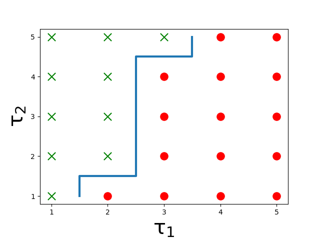
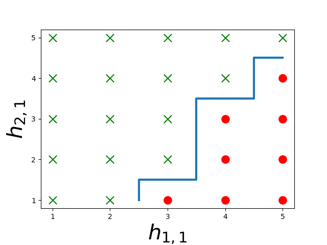
Many works have proved that optimal scheduling policies have the threshold structure in Definition 1 for different problems, where the reward of an individual user is a monotonic function of its state [5, 12, 13]. Our problem has the same property, where the estimation MSE of sensor $n$ decreases with the decreasing AoI state and the increasing channel state.

To verify whether the optimal policy of Problem 1 has the threshold structure, we consider a system with $N=2$ and $M=1$ and adopt the conventional value iteration algorithm to find the optimal policy. As illustrated in Fig. 2, we see action switching curves in both AoI and channel state spaces, and the properties in Definition 1 are observed. Due to space limitations, we here do not present formal proof that the optimal policy has a threshold structure, but will investigate it in our future work. In Section V, our numerical results also show that the optimized threshold policy is near optimal, confirming the conjecture.

For property (i), given that sensor $n$ is scheduled at channel $m$ at a certain state, if the channel quality of $h_{n,m}$ improves while the AoI and the other channel states are the same, then the threshold policy still assigns channel $m$ to sensor $n$. The property is reasonable since the channel quality of sensor $n$ to channel $m$ is the only factor changed and improved.

For property (ii), if the AoI state of sensor $n$ is increased while the other states remain the same, the policy must schedule sensor $n$ to a channel that is no worse than the previous one. Such a scheduling policy does make sense, since a larger sensor $n$’s AoI leads to a lower reward, requiring a better channel for transmission to improve the reward effectively.

In the following, we will develop novel schemes that leverage the threshold structure to guide DRL algorithms for solving Problem 1 with improved training speed and performance.

We define the Q-value as the expected discounted sum of the reward function

which measures the long-term performance of policy $\pi$ given the current state-action pair $(\mathbf{s}_{k},\mathbf{a}_{k})$. Let $\pi^{*}$ denote the optimal policy of Problem 1. Then, the corresponding Q-value can, in principle, be obtained by solving the Bellman equation [16]

From the definition (21), the optimal policy generates the best action achieving the highest Q-value, and can be written as

A well-trained DQN uses a neural network (NN) with the parameter set $\bm{\theta}$ to approximate the Q-values of the optimal policy in (23) as $Q(\mathbf{s}_{k},\mathbf{a}_{k};\bm{\theta})$ and use it to find the optimal action. Considering the action space defined in Section III-A, the DQN has $N!/(N-M)!$ Q-value outputs of different state-action pairs. To train the DQN, one needs to sample data (consisting of states, actions, rewards, and next states), define a loss function of $\bm{\theta}$ based on the collected data, and minimize the loss function to find the optimized $\bm{\theta}$. However, the conventional DQN training method has never utilized structures of optimal policies before.

To utilize the knowledge of the threshold policy structure for enhancing the DQN training performance, we propose 1) an SE action selection method based on Definition 1 to select reasonable actions and hence enhance the data sampling efficiency; and 2) an SE loss function definition to add the penalty to sampled actions that do not follow the threshold structure.

Our SE-DQN training algorithm has three stages: 1) the DQN with loose SE action selection stage, which only utilizes part of the structural property, 2) the DQN with tight SE action selection stage utilizes the full structural property, and 3) the conventional DQN stage. The first two stages use the SE action selection schemes and the SE loss function to train the DQN fast, resulting in a reasonable threshold policy, and the last stage is for further policy exploration. In what follows, we present the loose and tight SE action selection schemes and the SE loss function.

Different from the DQN, which has one NN to estimate the Q-value, a DDPG agent has two NNs [17], a critic NN with parameter $\bm{\theta}$ and an actor NN with the parameter $\bm{\mu}$. In particular, the actor NN approximates the optimal policy $\pi^{*}(\mathbf{s})$ by $\mu(\mathbf{s};\bm{\mu})$, while the critic NN approximates the Q-value of the optimal policy $Q^{*}(\mathbf{s},\mathbf{a})$ by $Q(\mathbf{s},\mathbf{a};\bm{\theta})$. In general, the critic NN judges whether the generated action of the actor NN is good or not, and the latter can be improved based on the former. The critic NN is updated by minimizing the TD error similar to the DQN. The actor-critic framework enables DDPG to solve MDPs with continuous and large action space, which cannot be handled by the DQN.

To solve our scheduling problem with a discrete action space, we adopt an action mapping scheme similar to the one adopted in [10]. We set the direct output of the actor NN with $N$ continuous values, ranging from $-1$ to $1$, corresponding to sensors $1$ to $N$, respectively. Recall that the DQN has $N!/(N-M)!$ outputs. The $N$ values are sorted in descending order. The sensors with the highest $M$ ranking are assigned to channels $1$ to $M$, respectively. The corresponding ranking values are then linearly normalized to $[-1,1]$ as the output of the final outputs of the actor NN, named as the virtual action $\mathbf{v}$. It directly follows that the virtual action $\mathbf{v}$ and the real scheduling action $\mathbf{a}$ can be mapped from one to the other directly. Therefore, we use the virtual action $\mathbf{v}$, instead of the real action $\mathbf{a}$, when presenting the SE-DDPG algorithm.

Similar to the SE-DQN, the SE-DDPG has the loose SE-DDPG stage, the tight SE-DDPG stage, and the conventional DDPG stage. The $i$th sampled transition is denoted as

We present the SE action selection method and the SE loss function in the sequel.

Our numerical experiments run on a computing platform with an Intel Core i5 9400F CPU @ 2.9 GHz with 16GB RAM and an NVIDIA RTX 2070 GPU. For the remote estimation system, we set the dimensions of the process state and the measurement as $l_{n}=2$ and $e_{n}=1$, respectively. The system matrices $\{\mathbf{A}_{n}\}$ are randomly generated with the spectral radius within the range of $(1,1.4)$. The entries of $\mathbf{C}_{n}$ are drawn uniformly from the range $(0,1)$, $\mathbf{W}_{n}$ and $\mathbf{V}_{n}$ are identity matrices. The fading channel state is quantized into $\bar{h}=5$ levels, and the corresponding packet drop probabilities are $0.2,0.15,0.1,0.05,$ and $0.01$. The distributions of the channel states of each sensor-channel pair $(n,m)$, i.e., $q^{(n,m)}_{1},\dots,q^{(n,m)}_{\bar{h}}$ are generated randomly.

During the training, we use the ADAM optimizer for calculating the gradient and reset the environment for each episode with $T=500$ steps. The episode numbers for the loose SE action, the tight SE action, and the conventional DQN stages are 50, 100, and 150, respectively. The settings of the hyperparameters for Algorithm 1 and Algorithm 2 are summarized in Table I.

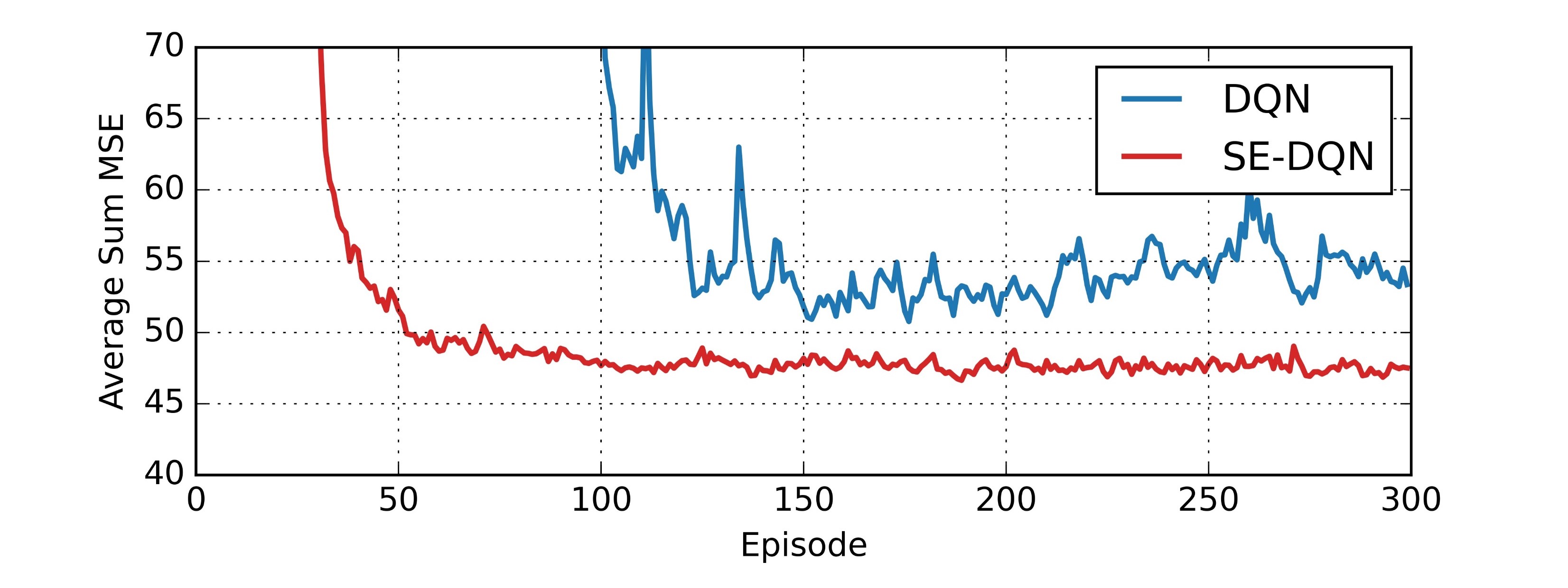
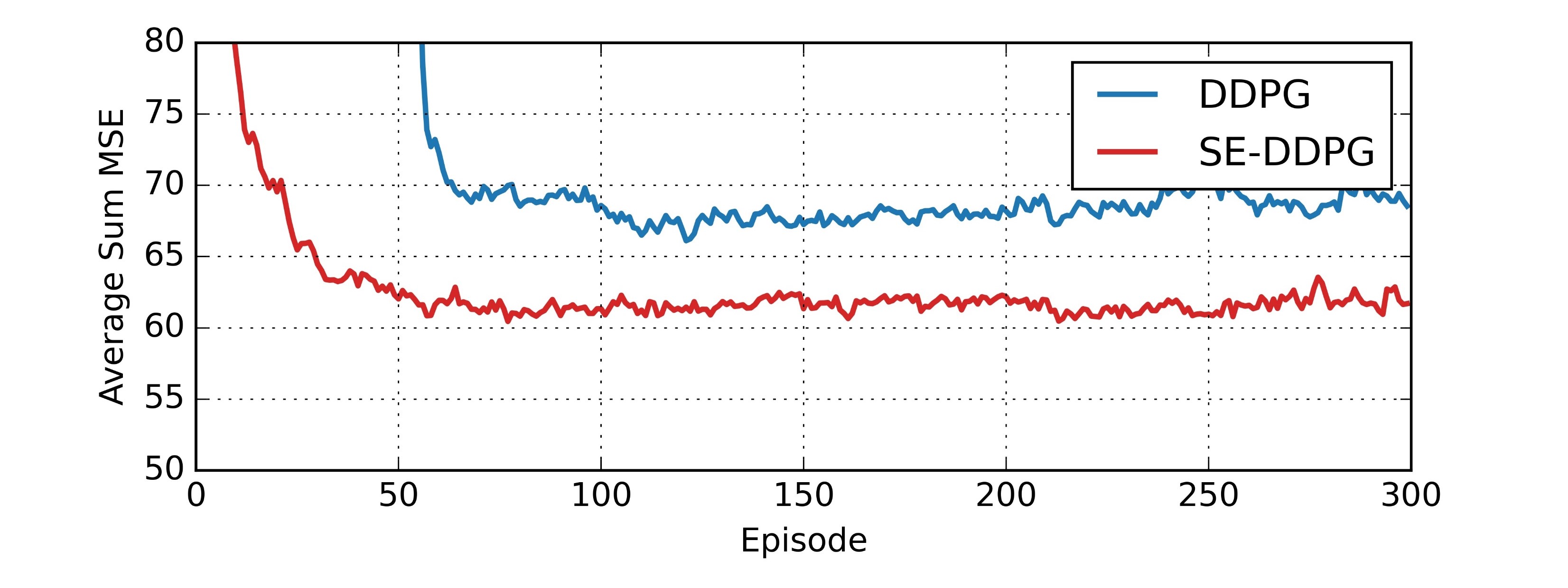
Fig. 3 and Fig. 4 illustrate the average sum MSE of all processes during the training achieved by the SE-DRL algorithms and the benchmarks under some system settings. Fig. 3 shows that the SE-DQN saves about $50\%$ training episodes for the convergence, and also decreases the average sum MSE for $10\%$ than the conventional DQN. Fig. 4 shows that the SE-DDPG saves about $30\%$ training episodes and reduces the average sum MSE by $10\%$, when compared to the conventional DDPG. Also, we see that the conventional DQN and DDPG stages (i.e. the last 150 episodes) in Fig 3 and 4 cannot improve much of the training performance. This implies that the SE stages have found near optimal policies.

In Table II, we test the performance of well-trained SE-DRL algorithms for different numbers of sensors and channels, and different settings of system parameters, i.e., $\mathbf{A}_{n}$, $\mathbf{C}_{n}$, and $q^{(n,m)}_{1},\dots,q^{(n,m)}_{\bar{h}}$, based on 10000-step simulations. We see that for 6-sensor-3-channel systems, the SE-DQN reduces the average MSE by $10\%$ to $25\%$ over DQN, while both DDPG and SE-DDPG achieve similar performance as the SE-DQN. This suggests that the SE-DQN is almost optimal and that the DDPG and the SE-DDPG cannot improve further. In 10-sensor-5-channel systems, neither the DQN nor the SE-DQN can converge, and the SE-DDPG achieves a $10\%$ MSE reduction over the DDPG. In particular, the SE-DDPG is the only converged algorithm in Experiment 12. In 20-sensor-10-channel systems, we see that the SE-DDPG can reduce the average MSE by $15\%$ to $25\%$. Therefore, the performance improvement of the SE-DDPG appears significant for large systems.

References

- [1] P. Park, S. Coleri Ergen, C. Fischione, C. Lu, and K. H. Johansson, “Wireless network design for control systems: A survey,” IEEE Commun. Surv. Tutor., vol. 20, no. 2, pp. 978–1013, May 2018.
- [2] K. Huang, W. Liu, Y. Li, B. Vucetic, and A. Savkin, “Optimal downlink-uplink scheduling of wireless networked control for industrial IoT,” IEEE Internet Things J., vol. 7, no. 3, pp. 1756–1772, Mar. 2020.
- [3] K. Gatsis, M. Pajic, A. Ribeiro, and G. J. Pappas, “Opportunistic control over shared wireless channels,” IEEE Trans. Autom. Control, vol. 60, no. 12, pp. 3140–3155, Mar, 2015.
- [4] D. Han, J. Wu, H. Zhang, and L. Shi, “Optimal sensor scheduling for multiple linear dynamical systems,” Automatica, vol. 75, pp. 260–270, Jan, 2017.
- [5] S. Wu, X. Ren, S. Dey, and L. Shi, “Optimal scheduling of multiple sensors over shared channels with packet transmission constraint,” Automatica, vol. 96, pp. 22–31, Oct. 2018.
- [6] R. S. Sutton and A. G. Barto, Reinforcement learning: An introduction. MIT press, 2018.
- [7] Z. Zhao, W. Liu, D. E. Quevedo, Y. Li, and B. Vucetic, “Deep learning for wireless networked systems: a joint estimation-control-scheduling approach,” arXiv preprint, Oct, 2022. [Online]. Available: https://doi.org/10.48550/arXiv.2210.00673
- [8] A. S. Leong, A. Ramaswamy, D. E. Quevedo, H. Karl, and L. Shi, “Deep reinforcement learning for wireless sensor scheduling in cyber–physical systems,” Automatica, vol. 113, pp. 1–8, Mar. 2020. Art. no. 108759.
- [9] W. Liu, K. Huang, D. E. Quevedo, B. Vucetic, and Y. Li, “Deep reinforcement learning for wireless scheduling in distributed networked control,” submitted to Automatica, 2021. [Online]. Available: https://doi.org/10.48550/arXiv.2109.12562
- [10] G. Pang, W. Liu, Y. Li, and B. Vucetic, “DRL-based resource allocation in remote state estimation,” arXiv preprint, May. 2022. [Online]. Available: https://doi.org/10.48550/arXiv.2205.12267
- [11] Z. D. Guo and E. Brunskill, “Directed exploration for reinforcement learning,” arXiv preprint, Jun 2019. [Online]. Available: https://doi.org/10.48550/arXiv.1906.07805
- [12] S. Wu, K. Ding, P. Cheng, and L. Shi, “Optimal scheduling of multiple sensors over lossy and bandwidth limited channels,” IEEE Trans. Netw. Syst., vol. 7, no. 3, pp. 1188–1200, Jan. 2020.
- [13] Y.-P. Hsu, E. Modiano, and L. Duan, “Age of information: Design and analysis of optimal scheduling algorithms,” in Proc. IEEE Int. Symp. Inf. Theory, June. 2017, pp. 561–565.
- [14] W. Liu, D. E. Quevedo, Y. Li, K. H. Johansson, and B. Vucetic, “Remote state estimation with smart sensors over Markov fading channels,” IEEE Trans. Autom. Control, vol. 67, no. 6, pp. 2743–2757, June, 2022.
- [15] W. Liu, D. E. Quevedo, K. H. Johansson, B. Vucetic, and Y. Li, “Stability conditions for remote state estimation of multiple systems over multiple markov fading channels,” IEEE Trans. Autom. Control, early access, Aug. 2022.
- [16] V. Mnih, K. Kavukcuoglu, D. Silver, A. Graves, I. Antonoglou, D. Wierstra, and M. Riedmiller, “Playing Atari with deep reinforcement learning,” in NIPS Deep Learning Workshop, 2013.
- [17] T. P. Lillicrap, et al., “Continuous control with deep reinforcement learning,” arXiv preprint, Sep. 2015. [Online]. Available: https://doi.org/10.48550/arXiv.1509.02971