Structure-Aware E(3)-Invariant Molecular Conformer Aggregation Networks
Abstract
A molecule’s 2D representation consists of its atoms, their attributes, and the molecule’s covalent bonds. A 3D (geometric) representation of a molecule is called a conformer and consists of its atom types and Cartesian coordinates. Every conformer has a potential energy, and the lower this energy, the more likely it occurs in nature. Most existing machine learning methods for molecular property prediction consider either 2D molecular graphs or 3D conformer structure representations in isolation. Inspired by recent work on using ensembles of conformers in conjunction with 2D graph representations, we propose (3)-invariant molecular conformer aggregation networks. The method integrates a molecule’s 2D representation with that of multiple of its conformers. Contrary to prior work, we propose a novel 2D–3D aggregation mechanism based on a differentiable solver for the Fused Gromov-Wasserstein Barycenter problem and the use of an efficient conformer generation method based on distance geometry. We show that the proposed aggregation mechanism is (3) invariant and propose an efficient GPU implementation. Moreover, we demonstrate that the aggregation mechanism helps to significantly outperform state-of-the-art molecule property prediction methods on established datasets. Our implementation is available at this link.
1 Introduction
Machine learning is increasingly used for modeling and analyzing properties of atomic systems with important applications in drug discovery and material design (Butler et al., 2018; Vamathevan et al., 2019; Choudhary et al., 2022; Fedik et al., 2022; Batatia et al., 2023). Most existing machine learning approaches to molecular property prediction either incorporate 2D (topological) (Kipf & Welling, 2017; Gilmer et al., 2017b; Xu et al., 2018; Veličković et al., 2018) or 3D (geometric) information of molecular structures (Schütt et al., 2017, 2021; Batzner et al., 2022; Batatia et al., 2022). 2D molecular graphs describe molecular connectivity (covalent bonds) but ignore the spatial arrangement of the atoms in a molecule (molecular conformation). 3D graph representations capture conformational changes but are commonly used to encode an individual conformer. Many molecular properties, such as solubility and binding affinity (Cao et al., 2022), however, inherently depend on a large number of conformations a molecule can occur as in nature, and employing a single geometry per molecule limits the applicability of machine-learning models. Furthermore, it is challenging to determine conformers that predominantly contribute to the molecular properties of interest. Thus, developing expressive representations for molecular systems when modeling their properties is an ongoing challenge.
To overcome this, recent work has introduced molecular representations that incorporate both 2D molecular graphs and 3D conformers (Zhu et al., 2023). These methods aim to encode various molecular structures, such as atom types, bond types, and spatial coordinates, leading to more comprehensive feature embeddings. The latest algorithms, including graph neural networks, attention mechanisms (Axelrod & Gómez-Bombarelli, 2023), and long short-term memory networks (Wang et al., 2024b), have demonstrated improved generalization capabilities in various molecular prediction tasks. Despite their effectiveness, these methods struggle to balance model complexity and performance and face scalability challenges mainly due to the computational cost of generating 3D conformers. These problems are exacerbated when using several conformers per system, underscoring the need for strategies to mitigate these limitations.
Contributions. We propose a new message-passing neural network architecture that integrates both 2D and ensembles of 3D molecular structures. The approach introduces a geometry-aware conformer ensemble aggregation strategy using Fused Gromov-Wasserstein (FGW) barycenters (Titouan et al., 2019), in which interactions between atoms across conformers are captured using both latent atom embeddings and conformer structures. The aggregation mechanism is invariant to actions of the group —the Euclidean group in 3 dimensions—such as translations, rotations, and inversion as well as to permutations of the input conformers. To make the proposed method applicable to large-scale problems, we accelerate the solvers for the FGW barycenter problem with entropic-based techniques (Rioux et al., 2023), allowing the model to be trained in parallel on multiple GPUs. We also experimentally explore the impact of the number of conformers and demonstrate that, within our framework, a modest number of conformers generated through efficient distance geometry-based sampling achieves state-of-the-art accuracy. We partially explain this through a theoretical analysis showing that the empirical barycenter converges to the target barycenter at a rate of , where denotes the number of conformers. Finally, we conduct a systematic evaluation of our proposed approaches, comparing their performance to state-of-the-art algorithms. The results show that our method is competitive and frequently surpasses existing methods across a variety of datasets and tasks.
2 Background
We first provide notations used in the paper. We note the simplex histogram with -bins as and as the set of symmetric matrices of size taking values in . For any , denotes the Dirac measure in . Let be the set of all probability measures on a space . We denote for any . We denote the matrix scalar product associated with the Forbenius norm as . The tensor-matrix multiplication will be denoted as , i.e., given any tensor and matrix , is the matrix .
A graph is a pair with finite sets of vertices or nodes and edges . We set and write that the graph is of order . For ease of notation, we denote the edge in by or . The neighborhood of in is denoted by and the degree of a vertex is . An attributed graph is a triple with a graph and (vertex-)feature (attribute) function , for some . Then is an attribute or feature of , for in . When we have multiple attributes, we have a pair , where and in is a node attribute matrix. For a matrix in and in , we denote by in the th row of such that . Analogously, we can define attributes for the edges of the graph. Furthermore, we can encode an -order graph via an adjacency matrix .
2.1 Message-Passing Neural Networks
Message-passing neural networks (MPNN) learn -dimensional real-valued vector representations for each vertex in a graph by exchanging and aggregating information from neighboring nodes. Each vertex is annotated with a feature in representing characteristics such as atom positions and numbers in the case of chemical molecules. In addition, each edge is associated with a feature vector . An MPNN architecture consists of a composition of permutation-equivariant parameterized functions.
Following Gilmer et al. (2017a) and Scarselli et al. (2009), in each layer, , we compute vertex features
| (1) |
where , , and are differentiable parameterized functions. In the case of graph-level regression problems, one uses
| (2) |
to compute a single vectorial representation based on learned vertex features after iteration where can be a differentiable parameterized function.
Molecules are -dimensional structures that can be represented by geometric graphs, capturing each atom’s 3D position. To obtain more expressive representations, we also consider geometric input attributes and focus on vectorial features of nodes. Since we address the problem of molecular property prediction, where we assume the properties to be invariant to actions of the group , we focus on -invariant MPNNs for geometric graphs.

2.2 Fused Gromov-Wasserstein Distance
Fused Gromov-Wasserstein. An undirected attributed graph of order in the optimal transport context is defined as a tuple , where is a node feature matrix and is a matrix encoding relationships between nodes, and denotes the probability measure of nodes within the graph, which can be modeled as the relative importance weights of graph nodes. Without any prior knowledge, uniform weights can be chosen (Vincent-Cuaz et al., 2022). The matrix can be the graph adjacency matrix, the shortest-path matrix or other distance metrics based on the graph topologies (Peyré et al., 2016; Titouan et al., 2019, 2020). Given two graphs of order , respectively, Fused Gromov-Wasserstein (FGW) distance can be defined as follows:
| (3) |
Here is the pairwise node distance matrix, the 4-tensor representing the alignment cost matrix, and is the set of all valid couplings between node distributions and . Moreover, is the distance metric in the feature space, and is the weight that trades off between the Gromov-Wasserstein cost on the graph structure and Wasserstein cost on the feature signal. In practice, we usually choose , Euclidean distance for , and to calculate FGW distance.
Entropic Fused Gromov-Wasserstein. The entropic FGW distance adds an entropic term (Cuturi, 2013) as
| (4) |
where the entropic scalar facilitates the tunable trade-off between solution accuracy and computational performance (w.r.t. lower and higher , respectively). Solving this entropic FGW involves iterations of solving the linear entropic OT problem Equation 37 with (stabilized) Sinkhorn projections (Proposition 2 (Peyré et al., 2016)), described in Appendix C and Algorithm 2.
3 ConAN: Conformer Aggregation Networks via Fused Gromov-Wasserstein Barycenters
In what follows, we refer to the representation of atoms and covalent bonds and their attributes as the 2D structure and the atoms, their 3D coordinates, and atom types as 3D structures. The following subsections describe each part of the framework in detail.
3.1 Conformer Generation
To efficiently generate conformers, we employ distance geometry-based algorithms, which convert distance constraints into Cartesian coordinates. For atomistic systems, constraints typically define lower and upper bounds on interatomic squared distances. In a 2D input graph, covalent bond distances adhere to known ranges, while bond angles are determined by corresponding geminal distances. Adjacent atoms or functional groups adhere to cis/trans limits for rotatable bonds or set values for rigid groups. Other distances have hard sphere lower bounds, usually chosen approximately 10 below van der Waals radii (Hawkins, 2017). Chirality constraints are applied to every rigid quadruple of atoms.
A distance geometry algorithm now randomly generates a -dimensional conformation satisfying the constraints. To bias the generation towards low-energy conformations, a simple and efficient force field is typically applied. We use efficient implementations from the RDKit package (Landrum, 2016).
3.2 Conformer Aggregation Network
We propose a new MPNN-based neural network that consists of three parts as depicted in Figure 1. First, a 2D MPNN model is used to capture the general molecular features such as covalent bond structure and atom features. Second, a novel FGW barycenter-based implicit -invariant aggregation function that integrates the representations of molecular 3D conformations computed by geometric message-passing neural networks. Finally, a permutation and -invariant aggregation function will be used to combine the 2D graph and 3D conformer representations of the molecules.
2D Molecular Graph Message-Passing Network. Each molecule is represented by a 2D graph with nodes representing its atoms and edges representing its covalent bonds, annotated with molecular features and , respectively (see Section 6 for details). To propagate features across a molecule and get 2D molecular representations, we use GAT layers, which utilize a self-attention mechanism in message-passing with the following operations:
| (5) |
and where are the GAT attention coefficients and a learnable parameter matrix. Following Veličković et al. (2018), the attention mechanism is implemented with a single-layer feedforward neural network. To obtain a per-molecule embedding, we compute , where is the number of message-passing layers.
3D Conformer Message-Passing Network. A conformer (atomic structure) of a molecule is defined as where is the number of atoms, are the Cartesian coordinates of atom , and is the atomic number of atom . We use weighted adjacency matrices to represent pairwise atom distances. In some cases we will apply a cutoff radius to these distances. We employ the geometric MPNN SchNet (Schütt et al., 2017), although it is worth noting that alternative -invariant neural networks could be seamlessly integrated. The selection of SchNet is motivated not only by its proficient balance between model complexity and efficacy but also by its proven utility in previous works (Axelrod & Gómez-Bombarelli, 2023). SchNet performs -invariant message-passing by using radial basis functions to incorporate the distances of the geometric node features . We refer the reader to Section D.1 for more details. We denote the matrix whose columns are the atom-wise features of SchNet from the last message-passing layer with , that is, .
To compute the vector representation for a conformer , we aggregate the atom-wise embeddings obtained from the last message-passing layer of SchNet into a single vector representation as , where is the set of atoms and and learned during training. For a set of conformers, the output of our 3D MPNN models is a matrix whose columns are the embeddings for conformer , that is, .
FGW Barycenter Aggregation. We now introduce an implicit and differentiable neural aggregation function whose output is determined by solving an FGW barycenter optimization problem. Its input is graphs for each conformer , with features computed by an -invariant MPNN, with weighted adjacency matrix of pairwise atomic distances, and the probability mass of each atom , typically set to . The output of the barycenter conformer, denoted as , represents the geometric mean of the input conformers, incorporating both their structural characteristics and features (Figure 1). The barycenter is the conformer graph that minimizes the sum of weighted FGW distances among the conformer graphs with feature matrices , structure matrices , and base histograms . That is, given any fixed and any , the FGW barycenter is defined as
| (6) |
where is the fused Gromov-Wasserstein distance defined in Equation 3, and where we set, for each pair of conformer graphs and , as the feature distance matrix, and as the 4-tensor representing the structural distance when aligning atoms to and to (Figure 2). Solving Equation 6, we obtain a unique FGW barycenter graph with representation for each atom . We aggregate the atom-wise embeddings obtained from the FGW barycenter into a single vector representation using .

Intuitively, barycenter-based aggregation in Eq.(6) can be seen as a more distance (structure) preserving pooling operation rather than standard mean aggregation. For instance, consider two conformers, where one is a 180-degree rotation of the other. Averaging their coordinates collapses the hydrogen atoms into the same position, creating an unphysical structure. On the contrary, employing the FGW Barycenter might prevent such issues.
Invariant Aggregation of 2D and 3D Representations. We integrate the representations of the 2D graph and the 3D conformer graphs using an average aggregation as well as the barycenter-based aggregation. The requirement for this aggregation is that it is invariant to the order of the input conformers; that is, it treats the conformers as a set as well as invariant to actions of the group .
Let and be the matrices whose columns are, respectively, copies of the 2D and barycenter representations from previous sections. Using learnable weight matrices , , and , we obtain the final atom-wise feature matrices as
| (7) |
where is a hyper-parameter controlling the contribution of the barycenter-based feature. Intuitively, this aggregation function, where we use multiple copies of the 2D graph and barycenter representations, provides a balanced contribution of the three types of representations and is empirically highly beneficial. Finally, to predict a molecular property, we apply a linear regression layer on a mean-aggregation of the per-conformations embedding as:
| (8) |
We can show that the function defined by Section 3.2 to Equation 8 is invariant to actions of the group and permutations acting on the sequence of input conformers.
Theorem 3.1.
Let be the 2D graph and with , , be a sequence of conformers of a molecule. Let be the function defined by Section 3.2 to Equation 8. For any we have that . Moreover, for any we have that .
4 Efficient and Convergent Molecular Conformer Aggregation
In this section, we provide some theoretical results to justify our novel FGW barycenter-based implicit -invariant aggregation function that integrates the representations of molecular 3D conformations computed by geometric message-passing neural networks in Section 3.2. We established a fast convergence rate of the empirical FGW barycenters to the true barycenters as a function of the number of conformer samples .
Undirected Attribute Graph Space. Let us define a structured object to be a triplet , , where and are feature and structure metric spaces, respectively, and is a probability measure over . By defining , the probability measure of the nodes, the graph represents a fully supported probability measure over the feature/structure of the product space, , which describes the entire undirected attributed graph. We note the set of all metric spaces. The space of all structured objects over will be written as , and is defined by all the triplets , where and .
True and Empirical Barycenters. Given , the variance functional of a distribution is defined as follows:
| (9) |
where is a true barycenter defined in equation (10). We will then restrict our attention to the subset . Note that is a subset of with finite variance and defined the same way as but on . For any , we define the true barycenter of is any s.t.
| (10) |
In our context of predicting molecular properties, the true barycenter is unknown. However, we can still draw random sample independently of the 3D molecular representation from . Then, an empirical barycenter is defined as a barycenter of the empirical distribution , i.e.,
| (11) |
4.1 Fast Convergence of Empirical FGW Barycenter
This work establishes a novel fast rate convergence for empirical barycenters in the FGW space via Theorem 4.1, which is proved in Appendix B. To the best of our knowledge, this is new in the literature, where only the result for Wasserstein space exists in Le Gouic et al. (2022).
Theorem 4.1.
Let be a probability measure on the 2-FGW space. Let and be barycenter and variance functional of satisfying (10) and (9), respectively. Let and suppose that every is the pushforward of by the gradient of an -strongly convex and smooth function , i.e., . If , then is unique and any empirical barycenter of satisfies
| (12) |
The upper bound in Equation 12 implies that the empirical barycenter converges to the target distribution at a rate of , where is the number of 3D conformers. This suggests utilizing small values of , such as , would yield a satisfactory approximation for . We confirm this empirically in experiments in Section 6.5.
4.2 Empirical Entropic FGW Barycenter
To train on large-scale problems, we propose to solve the entropic relaxation of Equation 6 to take advantage of GPU computing power (Peyré et al., 2019). Given a set of conformer graphs , we want to optimize the entropic barycenter , where we fixed the prior on nodes
| (13) |
with . Titouan et al. (2019) solve Equation 13 using Block Coordinate Descent, which iteratively minimizes the original FGW distance between the current barycenter and the graphs . In our case, we solve for couplings of entropic FGW distances to the graphs at each iteration, then following the update rule for structure matrix (Proposition 4, (Peyré et al., 2016))
| (14) |
and for the feature matrix (Titouan et al., 2019; Cuturi & Doucet, 2014)
| (15) |
leading to Algorithm 1. More details on practical implementations and algorithm complexity are in Appendix C.
5 Related Work
Molecular Representation Learning. The traditional approach for molecular representation referred to as connectivity fingerprints (Morgan, 1965) encodes the presence of different substructures within a compound in the form of a binary vector. Modern molecular representations used in machine learning for molecular properties prediction include 1D strings (Ahmad et al., 2022; Wang et al., 2019), 2D topological graphs (Gilmer et al., 2017a; Yang et al., 2019; Rong et al., 2020; Hu et al., 2020b) and 3D geometric graphs (Fang et al., 2021; Zhou et al., 2023; Liu et al., 2022a). The use of an ensemble of molecular conformations remains a relatively unexplored frontier in research, despite early evidence suggesting its efficacy in property prediction (Axelrod & Gómez-Bombarelli, 2023; Wang et al., 2024b). Another line of work uses conformers only at training time in a self-supervised loss to improve a 2D MPNN (Stärk et al., 2022). Contrary to prior work, we introduce a novel and streamlined barycenter-based conformer aggregation technique, seamlessly integrating learned representations from both 2D and 3D MPNNs. Moreover, we show that cost-effective conformers generated through distance-geometry sampling are sufficiently informative.
Geometric Graph Neural Networks. Graph Neural Networks (GNNs) designed for geometric graphs operate based on the message-passing framework, where the features of each node are dynamically updated through a process that respects permutation equivariance. Examples are models such as SphereNet (Liu et al., 2022b), GMNNs (Zaverkin & Kästner, 2020), DimeNet (Gasteiger et al., 2020b), GemNet-T (Gasteiger et al., 2021), SchNet (Schütt et al., 2017), GVP-GNN, PaiNN, E(n)-GNN (Satorras et al., 2021), MACE (Batatia et al., 2022), ICTP (Zaverkin et al., 2024), SEGNN (Brandstetter et al., 2022), SE(3)-Transformer (Fuchs et al., 2020), and VisNet (Wang et al., 2024a).
Optimal Transport in Graph Learning. By modeling graph features/structures as probability measures, the (Fused) GW distance (Titouan et al., 2020) serves as a versatile metric for comparing structured graphs. Previous applications of GW distance include graph node matching (Xu et al., 2019b), partitioning (Xu et al., 2019a; Chowdhury & Needham, 2021), and its use as a loss function for graph metric learning (Vincent-Cuaz et al., 2021, 2022; Chen et al., 2020; Zeng et al., 2023). More recently, FGW has been leveraged as an objective for encoding graphs (Tang et al., 2023) in tasks such as graph prediction (Brogat-Motte et al., 2022) and classification (Ma et al., 2023). To the best of our knowledge, we are the first to introduce the entropic FGW barycenter problem (Peyré et al., 2016; Titouan et al., 2020) for molecular representation learning. By employing the entropic formulation (Cuturi, 2013; Cuturi & Doucet, 2014), our learning pipeline enjoys a tunable trade-off between barycenter accuracy and computational performance, thus enabling an efficient hyperparameter tuning process. Moreover, we also present empirical barycenter-related theories, demonstrating how this entropic FGW barycenter framework effectively captures meaningful underlying structures of 3D conformers, thereby enhancing overall performance.
6 Experiments
6.1 Implementation Details
We encode each molecule in the SMILES format and employ the RDKit package to generate 3D conformers. We set the size of the latent dimensions of GAT (Veličković et al., 2018) to . Node features are initialized based on atomic properties such as atomic number, chirality, degree, charge, number of hydrogens, radical electrons, hybridization, aromaticity, and ring membership, while edges are represented as one-hot vectors denoting bond type, stereo configuration, and conjugation status. Each 3D conformer generated by RDKit comprises atoms with the corresponding 3D coordinates representing their spatial positions. Subsequently, we establish the graph structure and compute atomic embeddings utilizing the force-field energy-based SchNet model (Schütt et al., 2017), extracting features prior to the layer. Our SchNet configuration incorporates three interaction blocks with feature maps of size , employing a radial function defined on Gaussians spaced at intervals of with a cutoff distance of 10 . The output of each conformer forms a graph , utilized in solving the FGW barycenter as defined in Eq. (6). Subsequently, we aggregate features from 2D, 3D, and barycenter molecule graphs using Eqs. (7-8), followed by MLP layers. Leveraging Sinkhorn iterations in our barycenter solver (Algorithm 1), we speed up the training process across multiple GPUs using PyTorch’s distributed data-parallel technique. Training the entire model employs the Adam optimizer with initial learning rates selected from , halved using ReduceLROnPlateau after epochs without validation set improvement. Further experimental details are provided in the Appendix.
To accelerate the training process, especially in large-scale settings (e.g., BDE dataset), we first train the model with 2D and 3D features for some epochs, and then load the saved model and continue to train with full configurations as in Eq.(7) till converge. We set empirically in Eq.(7) is .
| Lipo | ESOL | FreeSolv | BACE | CoV-2 3CL | Cov-2 | BDE | |
|---|---|---|---|---|---|---|---|
| Train | 2940 | 789 | 449 | 1059 | 50 (485) | 53 (3294) | 8280 |
| Valid. | 420 | 112 | 64 | 151 | 15 (157) | 17 (1096) | 1184 |
| Test | 840 | 227 | 129 | 303 | 11 (162) | 22 (1086) | 2366 |
| Total | 4200 | 1128 | 642 | 1513 | 76 (804) | 92 (5476) | 11830 |
6.2 Molecular Property Prediction Tasks
Dataset. We use four datasets Lipo, ESOL, FreeSolv, and BACE in MoleculeNet benchmark (Table 1), spanning on various molecular characteristics such as physical chemistry and biophysics. We split data using random scaffold settings as baselines and reported the mean and standard deviation of mean square error (mse) by running on five trial times. More information for datasets is in Section D.2 Appendix.
Baselines. We compare against various benchmarks, including both supervised, pre-training, and multi-modal approaches. (i) The supervised methods are 2D graph neural network models including 2D-GAT (Veličković et al., 2018), D-MPNN (Yang et al., 2019), and AttentiveFP (Xiong et al., 2019); (ii) 2D molecule pretraining methods are PretrainGNN (Hu et al., 2020a), GROVER (Rong et al., 2020), MolCLR (Wang et al., 2022), ChemRL-Gem (Fang et al., 2022), ChemBERTa-2 (Ahmad et al., 2022), and MolFormer (Ross et al., 2022). It’s important to note that these models are pre-trained on a vast amount of data; for example, MolFormer is learned on billion molecules from PubChem and ZINC datasets. We also compare with the (iii) 2D-3D aggregation ConfNet model (Liu et al., 2021), which is one of the winners of KDD Cup on OGB Large-Scale Challenge (Hu et al., 2021). Finally, we benchmark with 3D conformers-based models such as UniMol (Zhou et al., 2023), SchNet, and ChemProp3D (Axelrod & Gómez-Bombarelli, 2023). Among this, UniMol is pre-trained on M molecular conformation and requires 11 conformers on each downstream task. We train SchNet with conformers ( for FreeSolv) and test with two versions: (a) taking output at the final layer and averaging different conformers (SchNet-scalar), (b) using feature node embeddings before layers and aggregating conformers by an MLP layer (SchNet-em). In ChemProp3D, we replace the classification header with an MLP layer for regression tasks, training with a 2D molecular graph and conformers. With the ConfNet, we use conformers in the training step and provide results for conformers for the evaluations step, followed by configurations in (Liu et al., 2021).
| Model | Lipo | ESOL | FreeSolv | BACE |
| 2D-GAT | ||||
| D-MPNN | ||||
| Attentive FP | - | |||
| PretrainGNN | - | |||
| GROVER_large | - | |||
| ChemBERTa-2* | - | |||
| ChemRL-GEM | - | |||
| MolFormer | ||||
| UniMol | - | |||
| SchNet-scalar | ||||
| SchNet-emb | ||||
| ChemProp3D | ||||
| ConfNet | - | |||
| ConAN | ||||
| ConAN-FGW |
Results. Table 2 presents the experimental findings of ConAN, alongside competitive methods, with the best results highlighted in bold. Baseline outcomes from prior studies (Zhou et al., 2023; Fang et al., 2022; Chang & Ye, 2023) are included, while performance for other models is provided through public codes. ConAN version denotes the aggregation of 2D and 3D features as per Eq. (7) without employing the barycenter, whereas ConAN-FGW signifies full configurations. We employ a number of conformers and for ConAN, and ConAN-FGW, respectively, based on validation results for Lipo, ESOL, FreeSolv, and BACE. From the experiments, several observations emerge: (i) ConAN proves more effective than relying solely on 2D or 3D, as shown by Conan’s performance, achieving second-best rankings on three datasets compared to models using only 2D (ChemRL-GEM) or 3D representations (UniMol). (ii) ConAN-FGW consistently outperforms baselines across all datasets, despite employing significantly fewer 3D conformers than ConAN. This underscores the importance of leveraging the barycenter to capture invariant 3D geometric characteristics.
6.3 3D SARS-CoV Molecular Classification Tasks
Dataset. We evaluate ConAN on two datasets Cov-2 3CL and Cov-2 (Table 1), focusing on molecular classification tasks. The same splitting for training and testing is followed (Axelrod & Gómez-Bombarelli, 2023). We also apply the CREST (Grimme, 2019) to filter generated conformers by RDKit as (Axelrod & Gómez-Bombarelli, 2023) for fair comparisons. Model performance is reported with the receiver operating characteristic area under the curve (ROC) and precision-recall area under the curve (PRC) over three trial times.
Baselines. We compare with three models, namely, SchNetFeatures, ChemProp3D, CP3D-NDU, each with two different attention mechanisms to ensemble 3D conformers and 2D molecular graph feature embedding as proposed by Axelrod & Gómez-Bombarelli (2023). These baselines generate conformers for their input algorithms. Additionally, the ConfNet (Liu et al., 2021) is also evaluated using or conformers in testing.
| Method | Num Conformers | Dataset | ROC | PRC |
|---|---|---|---|---|
| SchNetFeatures | 200 | CoV-2 3CL | 0.86 | 0.26 |
| ChemProp3D | 200 | CoV-2 3CL | 0.66 | 0.20 |
| CP3D-NDU | 200 | CoV-2 3CL | 0.901 | 0.413 |
| SchNetFeatures | average neighbors | CoV-2 3CL | 0.84 | 0.29 |
| ChemProp3D | average neighbors | CoV-2 3CL | 0.73 | 0.31 |
| CP3D-NDU | average neighbors | CoV-2 3CL | 0.916 | 0.467 |
| ConfNet | CoV-2 3CL | 0.493 | 0.128 | |
| ConAN | 10 | CoV-2 3CL | 0.881 0.009 | 0.317 0.052 |
| ConAN-FGW | 5 | CoV-2 3CL | 0.918 0.012 | 0.423 0.045 |
| SchNetFeatures | 200 | CoV-2 | 0.63 | 0.037 |
| ChemProp3D | 200 | CoV-2 | 0.53 | 0.032 |
| CP3D-NDU | 200 | CoV-2 | 0.663 | 0.06 |
| SchNetFeatures | average neighbors | CoV-2 | 0.61 | 0.027 |
| ChemProp3D | average neighbors | CoV-2 | 0.56 | 0.10 |
| CP3D-NDU | average neighbors | CoV-2 | 0.647 | 0.058 |
| ConfNet | CoV-2 | 0.501 0.001 | 0.36 0.2 | |
| ConAN | 10 | CoV-2 | 0.634 0.053 | 0.031 0.023 |
| ConAN-FGW | 10 | CoV-2 | 0.6735 0.032 | 0.036 0.014 |
Results. Table 3 presents performance of ConAN and ConAN-FGW with the number of conformers . It can be seen that ConAN-FGW delivers the best performance on ROC metric on two datasets and holds the second-best rank with PRC on CoV-2-3CL while requiring only conformers compared with conformers as CP3D-NDU. These results underscore the efficacy of incorporating barycenter components over merely aggregating 2D and 3D conformer embeddings, as observed in ConAN.
6.4 Molecular Conformer Ensemble Benchmark
Dataset. We run ConANon the BDE dataset (Table 1), which is the second-largest setting in (Zhu et al., 2023) aim to predict reaction-level molecule properties.
Baselines. ConAN is compared with state-of-the-art conformer ensemble strategies presented in Zhu et al. (2023), including SchNet (Schütt et al., 2017), DimeNet++ (Gasteiger et al., 2020a), GemNet (Gasteiger et al., 2021), PaiNN (Schütt et al., 2021), ClofNet (Du et al., 2022), and LEFTNet (Du et al., 2024). All these approaches employ conformers in training and testing. We provide two results of ConAN using only conformers and based on two architectures, SchNet and LEFTNet.
Results. Table 4 summarizes our achieved scores where the ConAN-FGW using LEFTNet backbone holds the second rank overall while using half the number of conformers. Additionally, it can be seen that ConAN-FGW improves with significant margins over both base models like SchNet () and LEFTNet (), demonstrating the generalization of the proposed aggregation.
| SchNet | DimeNet++ | GemNet | PainNN | ClofNet | LEFTNet | ConAN-FGW1 | ConAN-FGW2 | |
|---|---|---|---|---|---|---|---|---|
| Conf. | 20 | 20 | 20 | 20 | 20 | 20 | 10 | 10 |
| MAE | 1.9737 | 1.4741 | 1.6059 | 1.8744 | 2.0106 | 1.5276 | 1.6047 | 1.4829 |
6.5 Ablation Study
Contribution of 3D Conformer Number. One of the building blocks of our model is the use of multiple 3D conformations of a molecule. Each molecule is represented by conformations, so the choice of affects the model’s behavior. We treat as a hyperparameter and conduct experiments to validate the impact on model performance. To this end, we test on the ConAN version with different ( is equivalent to the 2D-GAT baseline) and report performance in Table 7 Appendix. We can observe that using 3D conformers with clearly improves performance compared to using only 2D molecular graphs as 2D-GAT. Furthermore, there is no straightforward dependency between the number of conformations in use and the accuracy of the model. For e.g., the performance tends to increase when using (Lipo and FreeSolv), but overall, the best trade-off value is .

Contribution of FGW Barycenter Aggregation. We examine the effect of barycenter aggregation when varying the number of conformers . Figure 3 summarizes results for those settings where we report average RMSE over four datasets in the MoleculeNet benchmark. We draw the following observations. First, ConAN-FGW shows notable enhancements as the number of conformers increases, with values ranging within the set ; however, when as , discernible disparities compared to the results obtained at diminish. We argue that this phenomenon aligns consistently with theoretical results in Theorem 4.1 suggesting that employing a sufficiently large facilitates a precise approximation of the target barycenter.
Secondly, upon examining various datasets, it becomes evident that ConAN-FGW consistently demonstrates enhanced performance with the utilization of larger conformers, a phenomenon not uniformly observed in the case of ConAN. This observation validates the robustness and resilience inherent in ConAN-FGW. We attribute this advantage to the efficacy of its geometry-informed aggregation strategy in ensemble learning with diverse 3D conformers.
Generalization to other Backbone Model. We investigate ConAN and ConAN-FGW performance using the VisNet backbone (Wang et al., 2024a), an equivariant geometry-enhanced graph neural network for 3D conformer embedding extraction. Results in Table 5 confirm that ConAN-FGW still advances ConAN performance. Between VisNet and SchNet, there is no universal best choice over datasets.
| Model | Lipo | ESOL | FreeSolv | BACE |
|---|---|---|---|---|
| ConAN (VisNet) | ||||
| ConAN-FGW | ||||
| ConAN (SchNet) | ||||
| ConAN-FGW |
6.6 3D Conformers distance distribution
We check diversity conformers randomly selected from a set of conformers generated by RDKit. For each pair of 3D conformers, we compute the optimal root mean square distance, which first aligns two molecules before measuring distance. Two settings are conducted: (i) estimating the mean, variance, max, and min distances distribution for conformers sampled by ConAN over conformers generated by RDKit. and (ii) estimate distribution for those values in case they are the top closest conformers. Figure 4 below shows our observation with a box plot on the validation set of Fressolv.

We observe that the distribution on the left ranges from 0.1 to 1.5, while in the worst case, the distance is between 0.01 and 0.08. Additionally, there’s a large gap between and on the left, whereas on the right, their means are close. It, therefore, can be seen that ConAN sampling strategy, given 200 RDKit-generated conformers, remains consistent and diverse.
6.7 FGW Barycenter Algorithm Efficiency
We contrast our entropic solver (Algorithm 1) with FGW-Mixup (Ma et al., 2023) for the barycenter problem. FGW-Mixup accelerates FGW problem-solving by relaxing coupling feasibility constraints. However, as the number of conformers increases, FGW-Mixup requires more outer iterations due to compounding marginal errors in solving FGW distances. In contrast, our approach employs an entropic-relaxation FGW formulation ensuring that marginal constraints are respected, resulting in a less noisy FGW subgradient. Furthermore, we implement our algorithm with distributed computation on multi-GPUs, as highlighted in Fig. 5. This figure illustrates epoch durations during both forward and backward steps of training, showcasing the performance across various conformer setups on FreeSolv and CoV-2 3CL datasets. Utilizing a batch size of 32 conformers, all three algorithms employ early termination upon reaching error tolerance. Notably, our solver exhibits linear scalability with , while FGW-Mixup shows exponential growth, presenting challenges for large-scale learning tasks. More details are in Section D.5.

7 Conclusion and Future Works
In this study, we present an -invariant molecular conformer aggregation network that integrates 2D molecular graphs, 3D conformers, and geometry-attributed structures using Fused Gromov-Wasserstein barycenter formulations. The results indicate the effectiveness of this approach, surpassing several baseline methods across diverse downstream tasks, including molecular property prediction and 3D classification. Moreover, we investigate the convergence properties of the empirical barycenter problem, demonstrating that an adequate number of conformers can yield a reliable approximation of the target structure. To enable training on large datasets, we also introduce entropic barycenter solvers, maximizing GPU utilization. Future research directions include exploring the robustness of using RDKit for multiple low-energy scenarios or more accurate reference methods for atomic structure relaxation, such as density-functional theory. Finally, extending ConAN, to learn from large-scale unlabeled multi-modal molecular datasets holds significant promise for advancing the field.
Acknowledgement
The authors thank the International Max Planck Research School for Intelligent Systems (IMPRS-IS) for supporting Duy M. H. Nguyen and Nina Lukashina. Duy M. H. Nguyen and Daniel Sonntag are also supported by the XAINES project (BMBF, 01IW20005), No-IDLE project (BMBF, 01IW23002), and the Endowed Chair of Applied Artificial Intelligence, Oldenburg University. An T. Le was supported by the German Research Foundation project METRIC4IMITATION (PE 2315/11-1). Nhat Ho acknowledges support from the NSF IFML 2019844 and the NSF AI Institute for Foundations of Machine Learning. Mathias Niepert acknowledges funding by Deutsche Forschungsgemeinschaft (DFG, German Research Foundation) under Germany’s Excellence Strategy - EXC and support by the Stuttgart Center for Simulation Science (SimTech). Furthermore, we acknowledge the support of the European Laboratory for Learning and Intelligent Systems (ELLIS) Unit Stuttgart.
Impact Statement
This paper presents work whose goal is to advance the field of Machine Learning, focusing on molecular representation learning. There are many potential societal consequences of our work, none of which we feel must be specifically highlighted here.
References
- Ahmad et al. (2022) Ahmad, W., Simon, E., Chithrananda, S., Grand, G., and Ramsundar, B. Chemberta-2: Towards chemical foundation models, 2022.
- Axelrod & Gómez-Bombarelli (2023) Axelrod, S. and Gómez-Bombarelli, R. Molecular machine learning with conformer ensembles. Mach. Learn.: Sci. Technol., 4(3):035025, September 2023. ISSN 2632-2153. doi: 10.1088/2632-2153/acefa7.
- Batatia et al. (2022) Batatia, I., Kovacs, D. P., Simm, G., Ortner, C., and Csanyi, G. Mace: Higher order equivariant message passing neural networks for fast and accurate force fields. In Koyejo, S., Mohamed, S., Agarwal, A., Belgrave, D., Cho, K., and Oh, A. (eds.), Advances in Neural Information Processing Systems, volume 35, pp. 11423–11436. Curran Associates, Inc., 2022.
- Batatia et al. (2023) Batatia, I., Benner, P., Chiang, Y., Elena, A. M., Kovács, D. P., Riebesell, J., Advincula, X. R., Asta, M., Baldwin, W. J., Bernstein, N., Bhowmik, A., Blau, S. M., Cărare, V., Darby, J. P., De, S., Pia, F. D., Deringer, V. L., Elijošius, R., El-Machachi, Z., Fako, E., Ferrari, A. C., Genreith-Schriever, A., George, J., Goodall, R. E. A., Grey, C. P., Han, S., Handley, W., Heenen, H. H., Hermansson, K., Holm, C., Jaafar, J., Hofmann, S., Jakob, K. S., Jung, H., Kapil, V., Kaplan, A. D., Karimitari, N., Kroupa, N., Kullgren, J., Kuner, M. C., Kuryla, D., Liepuoniute, G., Margraf, J. T., Magdău, I.-B., Michaelides, A., Moore, J. H., Naik, A. A., Niblett, S. P., Norwood, S. W., O’Neill, N., Ortner, C., Persson, K. A., Reuter, K., Rosen, A. S., Schaaf, L. L., Schran, C., Sivonxay, E., Stenczel, T. K., Svahn, V., Sutton, C., van der Oord, C., Varga-Umbrich, E., Vegge, T., Vondrák, M., Wang, Y., Witt, W. C., Zills, F., and Csányi, G. A foundation model for atomistic materials chemistry, 2023.
- Batzner et al. (2022) Batzner, S., Musaelian, A., Sun, L., Geiger, M., Mailoa, J. P., Kornbluth, M., Molinari, N., Smidt, T. E., and Kozinsky, B. E(3)-equivariant graph neural networks for data-efficient and accurate interatomic potentials. Nat. Commun., 13(1):2453, May 2022. ISSN 2041-1723.
- Brandstetter et al. (2022) Brandstetter, J., Hesselink, R., van der Pol, E., Bekkers, E. J., and Welling, M. Geometric and physical quantities improve e(3) equivariant message passing. In International Conference on Learning Representations, 2022.
- Brogat-Motte et al. (2022) Brogat-Motte, L., Flamary, R., Brouard, C., Rousu, J., and D’Alché-Buc, F. Learning to Predict Graphs with Fused Gromov-Wasserstein Barycenters. In Chaudhuri, K., Jegelka, S., Song, L., Szepesvari, C., Niu, G., and Sabato, S. (eds.), Proceedings of the 39th International Conference on Machine Learning, volume 162 of Proceedings of Machine Learning Research, pp. 2321–2335. PMLR, July 2022.
- Butler et al. (2018) Butler, K. T., Davies, D. W., Cartwright, H., Isayev, O., and Walsh, A. Machine learning for molecular and materials science. Nature, 559(7715):547–555, Jul 2018. ISSN 1476-4687.
- Cao et al. (2022) Cao, L., Coventry, B., Goreshnik, I., Huang, B., Sheffler, W., Park, J. S., Jude, K. M., Marković, I., Kadam, R. U., Verschueren, K. H., et al. Design of protein-binding proteins from the target structure alone. Nature, 605(7910):551–560, 2022.
- Chang & Ye (2023) Chang, J. and Ye, J. C. Bidirectional generation of structure and properties through a single molecular foundation model. arXiv preprint arXiv:2211.10590, 2023.
- Chen et al. (2020) Chen, B., Bécigneul, G., Ganea, O.-E., Barzilay, R., and Jaakkola, T. Optimal transport graph neural networks. arXiv preprint arXiv:2006.04804, 2020.
- Choudhary et al. (2022) Choudhary, K., DeCost, B., Chen, C., Jain, A., Tavazza, F., Cohn, R., Park, C. W., Choudhary, A., Agrawal, A., Billinge, S. J. L., Holm, E., Ong, S. P., and Wolverton, C. Recent advances and applications of deep learning methods in materials science. npj Comput. Mater., 8(1):59, Apr 2022. ISSN 2057-3960.
- Chowdhury & Needham (2021) Chowdhury, S. and Needham, T. Generalized spectral clustering via gromov-wasserstein learning. In International Conference on Artificial Intelligence and Statistics, pp. 712–720. PMLR, 2021.
- Cuturi (2013) Cuturi, M. Sinkhorn distances: Lightspeed computation of optimal transport. Advances in neural information processing systems, 26, 2013.
- Cuturi & Doucet (2014) Cuturi, M. and Doucet, A. Fast computation of wasserstein barycenters. In International conference on machine learning, pp. 685–693. PMLR, 2014.
- Du et al. (2022) Du, W., Zhang, H., Du, Y., Meng, Q., Chen, W., Zheng, N., Shao, B., and Liu, T.-Y. Se (3) equivariant graph neural networks with complete local frames. In International Conference on Machine Learning, pp. 5583–5608. PMLR, 2022.
- Du et al. (2024) Du, Y., Wang, L., Feng, D., Wang, G., Ji, S., Gomes, C. P., Ma, Z.-M., et al. A new perspective on building efficient and expressive 3d equivariant graph neural networks. Advances in Neural Information Processing Systems, 36, 2024.
- Ellinger et al. (2020) Ellinger, B., Bojkova, D., Zaliani, A., Cinatl, J., Claussen, C., Westhaus, S., Reinshagen, J., Kuzikov, M., Wolf, M., Geisslinger, G., Gribbon, P., and Ciesek, S. Identification of inhibitors of sars-cov-2 in-vitro cellular toxicity in human (caco-2) cells using a large scale drug repurposing collection, 2020.
- Fang et al. (2021) Fang, X., Liu, L., Lei, J., He, D., Zhang, S., Zhou, J., Wang, F., Wu, H., and Wang, H. Chemrl-gem: Geometry enhanced molecular representation learning for property prediction. Nature Machine Intelligence, 2021. doi: 10.48550/ARXIV.2106.06130.
- Fang et al. (2022) Fang, X., Liu, L., Lei, J., He, D., Zhang, S., Zhou, J., Wang, F., Wu, H., and Wang, H. Geometry-enhanced molecular representation learning for property prediction. Nature Machine Intelligence, 4(2):127–134, 2022.
- Fedik et al. (2022) Fedik, N., Zubatyuk, R., Kulichenko, M., Lubbers, N., Smith, J. S., Nebgen, B., Messerly, R., Li, Y. W., Boldyrev, A. I., Barros, K., Isayev, O., and Tretiak, S. Extending machine learning beyond interatomic potentials for predicting molecular properties. Nat. Rev. Chem., 6(9):653–672, Sep 2022. ISSN 2397-3358. doi: 10.1038/s41570-022-00416-3.
- Feydy et al. (2019) Feydy, J., Séjourné, T., Vialard, F.-X., Amari, S.-i., Trouvé, A., and Peyré, G. Interpolating between optimal transport and mmd using sinkhorn divergences. In The 22nd International Conference on aRtIfIcIaL InTeLlIgEnCe and Statistics, pp. 2681–2690. PMLR, 2019.
- Fuchs et al. (2020) Fuchs, F., Worrall, D., Fischer, V., and Welling, M. Se(3)-transformers: 3d roto-translation equivariant attention networks. In Larochelle, H., Ranzato, M., Hadsell, R., Balcan, M., and Lin, H. (eds.), Advances in Neural Information Processing Systems, volume 33, pp. 1970–1981. Curran Associates, Inc., 2020.
- Gasteiger et al. (2020a) Gasteiger, J., Groß, J., and Günnemann, S. Directional message passing for molecular graphs. International Conference on Learning Representations, 2020a.
- Gasteiger et al. (2020b) Gasteiger, J., Groß, J., and Günnemann, S. Directional message passing for molecular graphs. In International Conference on Learning Representations (ICLR), 2020b.
- Gasteiger et al. (2021) Gasteiger, J., Becker, F., and Günnemann, S. Gemnet: Universal directional graph neural networks for molecules. In Beygelzimer, A., Dauphin, Y., Liang, P., and Vaughan, J. W. (eds.), Advances in Neural Information Processing Systems, 2021.
- Gilmer et al. (2017a) Gilmer, J., Schoenholz, S. S., Riley, P. F., Vinyals, O., and Dahl, G. E. Neural message passing for quantum chemistry. In International Conference on Machine Learning, pp. 1263–1272, 2017a.
- Gilmer et al. (2017b) Gilmer, J., Schoenholz, S. S., Riley, P. F., Vinyals, O., and Dahl, G. E. Neural message passing for quantum chemistry. In Precup, D. and Teh, Y. W. (eds.), Proceedings of the 34th ICML, volume 70 of Proceedings of Machine Learning Research, pp. 1263–1272. PMLR, 06–11 Aug 2017b.
- Grimme (2019) Grimme, S. Exploration of chemical compound, conformer, and reaction space with meta-dynamics simulations based on tight-binding quantum chemical calculations. Journal of chemical theory and computation, 15(5):2847–2862, 2019.
- Hawkins (2017) Hawkins, P. C. Conformation generation: the state of the art. Journal of chemical information and modeling, 57(8):1747–1756, 2017.
- Hu et al. (2020a) Hu, W., Liu, B., Gomes, J., Zitnik, M., Liang, P., Pande, V., and Leskovec, J. Strategies for pre-training graph neural networks. In International Conference on Learning Representations, 2020a.
- Hu et al. (2020b) Hu, W., Liu, B., Gomes, J., Zitnik, M., Liang, P., Pande, V., and Leskovec, J. Strategies for pre-training graph neural networks. In International Conference on Learning Representations, 2020b.
- Hu et al. (2021) Hu, W., Fey, M., Ren, H., Nakata, M., Dong, Y., and Leskovec, J. Ogb-lsc: A large-scale challenge for machine learning on graphs. arXiv preprint arXiv:2103.09430, 2021.
- Kipf & Welling (2017) Kipf, T. N. and Welling, M. Semi-supervised classification with graph convolutional networks. In International Conference on Learning Representations, 2017.
- Landrum (2016) Landrum, G. Rdkit: open-source cheminformatics http://www. rdkit. org. 3(8), 2016.
- Le et al. (2022) Le, K., Le, D., Nguyen, H., Do, D., Pham, T., and Ho, N. Entropic Gromov-Wasserstein between Gaussian distributions. In ICML, 2022.
- Le Gouic et al. (2022) Le Gouic, T., Paris, Q., Rigollet, P., and Stromme, A. J. Fast convergence of empirical barycenters in Alexandrov spaces and the Wasserstein space. Journal of the European Mathematical Society, 25(6):2229–2250, May 2022. ISSN 1435-9855.
- Lin et al. (2020) Lin, T., Ho, N., Chen, X., Cuturi, M., and Jordan, M. I. Fixed-support Wasserstein barycenters: Computational hardness and fast algorithm. In NeurIPS, pp. 5368–5380, 2020.
- Liu et al. (2021) Liu, M., Fu, C., Zhang, X., Wang, L., Xie, Y., Yuan, H., Luo, Y., Xu, Z., Xu, S., and Ji, S. Fast quantum property prediction via deeper 2d and 3d graph networks. arXiv preprint arXiv:2106.08551, 2021.
- Liu et al. (2022a) Liu, S., Wang, H., Liu, W., Lasenby, J., Guo, H., and Tang, J. Pre-training molecular graph representation with 3d geometry. In International Conference on Learning Representations, 2022a.
- Liu et al. (2022b) Liu, Y., Wang, L., Liu, M., Lin, Y., Zhang, X., Oztekin, B., and Ji, S. Spherical message passing for 3d molecular graphs. In International Conference on Learning Representations, 2022b.
- Ma et al. (2023) Ma, X., Chu, X., Wang, Y., Lin, Y., Zhao, J., Ma, L., and Zhu, W. Fused gromov-wasserstein graph mixup for graph-level classifications. In Thirty-seventh Conference on Neural Information Processing Systems, 2023.
- Meyer et al. (2018) Meyer, B., Sawatlon, B., Heinen, S., Von Lilienfeld, O. A., and Corminboeuf, C. Machine learning meets volcano plots: computational discovery of cross-coupling catalysts. Chemical science, 9(35):7069–7077, 2018.
- Morgan (1965) Morgan, H. L. The generation of a unique machine description for chemical structures-a technique developed at chemical abstracts service. Journal of Chemical Documentation, 5(2):107–113, May 1965. ISSN 1541-5732. doi: 10.1021/c160017a018.
- Neyshabur et al. (2013) Neyshabur, B., Khadem, A., Hashemifar, S., and Arab, S. S. Netal: a new graph-based method for global alignment of protein–protein interaction networks. Bioinformatics, 29(13):1654–1662, 2013.
- Paszke et al. (2017) Paszke, A., Gross, S., Chintala, S., Chanan, G., Yang, E., DeVito, Z., Lin, Z., Desmaison, A., Antiga, L., and Lerer, A. Automatic differentiation in pytorch. In NIPS 2017 Workshop on Autodiff, 2017.
- Peyré (2015) Peyré, G. Entropic approximation of wasserstein gradient flows. SIAM Journal on Imaging Sciences, 8(4):2323–2351, 2015.
- Peyré et al. (2016) Peyré, G., Cuturi, M., and Solomon, J. Gromov-wasserstein averaging of kernel and distance matrices. In International conference on machine learning, pp. 2664–2672. PMLR, 2016.
- Peyré et al. (2019) Peyré, G., Cuturi, M., et al. Computational optimal transport: With applications to data science. Foundations and Trends® in Machine Learning, 11(5-6):355–607, 2019.
- Peyré et al. (2016) Peyré, G., Cuturi, M., and Solomon, J. Gromov-Wasserstein Averaging of Kernel and Distance Matrices. In Balcan, M. F. and Weinberger, K. Q. (eds.), Proceedings of The 33rd International Conference on Machine Learning, volume 48 of Proceedings of Machine Learning Research, pp. 2664–2672, New York, New York, USA, June 2016. PMLR.
- Rioux et al. (2023) Rioux, G., Goldfeld, Z., and Kato, K. Entropic gromov-wasserstein distances: Stability, algorithms, and distributional limits. arXiv preprint arXiv:2306.00182, 2023.
- Rong et al. (2020) Rong, Y., Bian, Y., Xu, T., Xie, W., Wei, Y., Huang, W., and Huang, J. Self-supervised graph transformer on large-scale molecular data. Advances in Neural Information Processing Systems, 33:12559–12571, 2020.
- Ross et al. (2022) Ross, J., Belgodere, B., Chenthamarakshan, V., Padhi, I., Mroueh, Y., and Das, P. Large-scale chemical language representations capture molecular structure and properties. Nature Machine Intelligence, 4(12):1256–1264, 2022.
- Satorras et al. (2021) Satorras, V. G., Hoogeboom, E., and Welling, M. E(n) equivariant graph neural networks. In Meila, M. and Zhang, T. (eds.), Proceedings of the 38th International Conference on Machine Learning, volume 139 of Proceedings of Machine Learning Research, pp. 9323–9332. PMLR, 18–24 Jul 2021.
- Scarselli et al. (2009) Scarselli, F., Gori, M., Tsoi, A. C., Hagenbuchner, M., and Monfardini, G. The graph neural network model. IEEE Transactions on Neural Networks, 20(1):61–80, 2009.
- Schmitzer (2019) Schmitzer, B. Stabilized sparse scaling algorithms for entropy regularized transport problems. SIAM Journal on Scientific Computing, 41(3):A1443–A1481, 2019.
- Schütt et al. (2017) Schütt, K., Kindermans, P., Felix, H. E. S., Chmiela, S., Tkatchenko, A., and Müller, K. Schnet: A continuous-filter convolutional neural network for modeling quantum interactions. In Advances in Neural Information Processing Systems 30: Annual Conference on Neural Information Processing Systems 2017, December 4-9, 2017, Long Beach, CA, USA, pp. 991–1001, 2017.
- Schütt et al. (2017) Schütt, K., Kindermans, P.-J., Sauceda Felix, H. E., Chmiela, S., Tkatchenko, A., and Müller, K.-R. Schnet: A continuous-filter convolutional neural network for modeling quantum interactions. In Guyon, I., Luxburg, U. V., Bengio, S., Wallach, H., Fergus, R., Vishwanathan, S., and Garnett, R. (eds.), Advances in Neural Information Processing Systems, volume 30. Curran Associates, Inc., 2017.
- Schütt et al. (2021) Schütt, K. T., Unke, O. T., and Gastegger, M. Equivariant message passing for the prediction of tensorial properties and molecular spectra. ICML, pp. 1–13, 2021.
- Source (2020) Source, D. L. Main protease structure and xchem fragment screen, 2020.
- Stärk et al. (2022) Stärk, H., Beaini, D., Corso, G., Tossou, P., Dallago, C., Günnemann, S., and Lió, P. 3D infomax improves GNNs for molecular property prediction. In Chaudhuri, K., Jegelka, S., Song, L., Szepesvari, C., Niu, G., and Sabato, S. (eds.), Proceedings of the 39th International Conference on Machine Learning, volume 162 of Proceedings of Machine Learning Research, pp. 20479–20502. PMLR, 17–23 Jul 2022.
- Tang et al. (2023) Tang, J., Zhao, K., and Li, J. A fused gromov-wasserstein framework for unsupervised knowledge graph entity alignment. arXiv preprint arXiv:2305.06574, 2023.
- Titouan et al. (2019) Titouan, V., Courty, N., Tavenard, R., Laetitia, C., and Flamary, R. Optimal Transport for structured data with application on graphs. In Chaudhuri, K. and Salakhutdinov, R. (eds.), Proceedings of the 36th International Conference on Machine Learning, volume 97 of Proceedings of Machine Learning Research, pp. 6275–6284. PMLR, June 2019.
- Titouan et al. (2020) Titouan, V., Chapel, L., Flamary, R., Tavenard, R., and Courty, N. Fused Gromov-Wasserstein Distance for Structured Objects. Algorithms, 13(9):212, August 2020. ISSN 1999-4893. doi: 10.3390/a13090212.
- Touret et al. (2020) Touret, F., Gilles, M., Barral, K., and et al. In vitro screening of a fda approved chemical library reveals potential inhibitors of sars-cov-2 replication. Sci Rep, 10:13093, 2020. doi: 10.1038/s41598-020-70143-6.
- Vamathevan et al. (2019) Vamathevan, J., Clark, D., Czodrowski, P., Dunham, I., Ferran, E., Lee, G., Li, B., Madabhushi, A., Shah, P., Spitzer, M., and Zhao, S. Applications of machine learning in drug discovery and development. Nat. Rev. Drug Discov., 18(6):463–477, Jun 2019. ISSN 1474-1784.
- Veličković et al. (2018) Veličković, P., Cucurull, G., Casanova, A., Romero, A., Liò, P., and Bengio, Y. Graph attention networks. In International Conference on Learning Representations, 2018.
- Veličković et al. (2018) Veličković, P., Cucurull, G., Casanova, A., Romero, A., Liò, P., and Bengio, Y. Graph attention networks. In ICLR, 2018.
- Vincent-Cuaz et al. (2021) Vincent-Cuaz, C., Vayer, T., Flamary, R., Corneli, M., and Courty, N. Online graph dictionary learning. In International conference on machine learning, pp. 10564–10574. PMLR, 2021.
- Vincent-Cuaz et al. (2022) Vincent-Cuaz, C., Flamary, R., Corneli, M., Vayer, T., and Courty, N. Template based Graph Neural Network with Optimal Transport Distances. In Koyejo, S., Mohamed, S., Agarwal, A., Belgrave, D., Cho, K., and Oh, A. (eds.), Advances in Neural Information Processing Systems, volume 35, pp. 11800–11814. Curran Associates, Inc., 2022.
- Wang et al. (2019) Wang, S., Guo, Y., Wang, Y., Sun, H., and Huang, J. Smiles-bert: Large scale unsupervised pre-training for molecular property prediction. In Proceedings of the 10th ACM International Conference on Bioinformatics, Computational Biology and Health Informatics, BCB ’19, pp. 429–436, New York, NY, USA, 2019. Association for Computing Machinery. ISBN 9781450366663. doi: 10.1145/3307339.3342186.
- Wang et al. (2022) Wang, Y., Wang, J., Cao, Z., and Barati Farimani, A. Molecular contrastive learning of representations via graph neural networks. Nature Machine Intelligence, 4(3):279–287, 2022.
- Wang et al. (2024a) Wang, Y., Wang, T., Li, S., He, X., Li, M., Wang, Z., Zheng, N., Shao, B., and Liu, T.-Y. Enhancing geometric representations for molecules with equivariant vector-scalar interactive message passing. Nature Communications, 15(1):313, 2024a.
- Wang et al. (2024b) Wang, Z., Jiang, T., Wang, J., and Xuan, Q. Multi-modal representation learning for molecular property prediction: Sequence, graph, geometry. arXiv preprint arXiv:2401.03369, 2024b.
- Wu et al. (2018) Wu, Z., Ramsundar, B., Feinberg, E. N., Gomes, J., Geniesse, C., Pappu, A. S., Leswing, K., and Pande, V. MoleculeNet: A benchmark for molecular machine learning. Chemical Science, pp. 513–530, 2018.
- Xiong et al. (2019) Xiong, Z., Wang, D., Liu, X., Zhong, F., Wan, X., Li, X., Li, Z., Luo, X., Chen, K., Jiang, H., et al. Pushing the boundaries of molecular representation for drug discovery with the graph attention mechanism. Journal of medicinal chemistry, 63(16):8749–8760, 2019.
- Xu et al. (2019a) Xu, H., Luo, D., and Carin, L. Scalable gromov-wasserstein learning for graph partitioning and matching. Advances in neural information processing systems, 32, 2019a.
- Xu et al. (2019b) Xu, H., Luo, D., Zha, H., and Duke, L. C. Gromov-wasserstein learning for graph matching and node embedding. In International conference on machine learning, pp. 6932–6941. PMLR, 2019b.
- Xu et al. (2018) Xu, K., Li, C., Tian, Y., Sonobe, T., Kawarabayashi, K.-i., and Jegelka, S. Representation learning on graphs with jumping knowledge networks. In Dy, J. and Krause, A. (eds.), Proceedings of the 35th International Conference on Machine Learning, volume 80 of Proceedings of Machine Learning Research, pp. 5453–5462. PMLR, 10–15 Jul 2018.
- Yang et al. (2019) Yang, K., Swanson, K., Jin, W., Coley, C., Eiden, P., Gao, H., Guzman-Perez, A., Hopper, T., Kelley, B., Mathea, M., Palmer, A., Settels, V., Jaakkola, T., Jensen, K., and Barzilay, R. Analyzing learned molecular representations for property prediction. Journal of Chemical Information and Modeling, 59(8):3370–3388, July 2019. ISSN 1549-960X. doi: 10.1021/acs.jcim.9b00237.
- Zaverkin & Kästner (2020) Zaverkin, V. and Kästner, J. Gaussian moments as physically inspired molecular descriptors for accurate and scalable machine learning potentials. Journal of Chemical Theory and Computation, 16(8):5410–5421, 2020. doi: 10.1021/acs.jctc.0c00347.
- Zaverkin et al. (2024) Zaverkin, V., Alesiani, F., Maruyama, T., Errica, F., Christiansen, H., Takamoto, M., Weber, N., and Niepert, M. Higher-rank irreducible Cartesian tensors for equivariant message passing, 2024.
- Zeng et al. (2023) Zeng, Z., Zhu, R., Xia, Y., Zeng, H., and Tong, H. Generative graph dictionary learning. In International Conference on Machine Learning, pp. 40749–40769. PMLR, 2023.
- Zhou et al. (2023) Zhou, G., Gao, Z., Ding, Q., Zheng, H., Xu, H., Wei, Z., Zhang, L., and Ke, G. Uni-mol: A universal 3d molecular representation learning framework. In The Eleventh International Conference on Learning Representations, 2023.
- Zhu et al. (2023) Zhu, Y., Hwang, J., Adams, K., Liu, Z., Nan, B., Stenfors, B., Du, Y., Chauhan, J., Wiest, O., Isayev, O., Coley, C. W., Sun, Y., and Wang, W. Learning over molecular conformer ensembles: Datasets and benchmarks, 2023.
Structure-Aware E(3)-Invariant Molecular Conformer Aggregation Networks Supplementary Material
In this supplementary material, we first present rigorous proofs for results concerning the E(3) invariant of the proposed aggregation mechanism in Appendix A, while those for the fast convergence of the empirical FGW barycenter are then provided in Appendix B. The entropic FGW algorithm and practical GPU considerations are then given in more detail in Appendix C. Finally, some experiment configuration supplements on SchNet neural architecture, 3D conformers generation and comparison between entropic FGW and FGW-mixup are deffered in Appendix D.
Appendix A Proof of Theorem 3.1
We will proceed as follows. First, we prove that is invariant to permutations of the input conformers and actions of the group applied to the input conformers. is invariant to the order of the input conformers by definition of the barycenter which is invariant to the order of the input graphs. Moreover, since by definition, actions of the group preserve distances between points in a -dimensional space and, by assumption, the upstream 3D MPNN is invariant to actions of , for any input conformer and its corresponding graph and any action we have that . is invariant to actions of the group because the 3D MPNN is invariant to actions of the group. is invariant due to distances between points being invariant. Hence, the input graphs to the barycenter optimization problem are invariant to actions of the group on the conformers and, therefore, the output barycenters are invariant to such group actions.
We know now for Equation 7: , that is invariant to both actions of the group and permutations of the input conformers. We also know that is equivariant to permutations of the input conformers, that is, every permutation of the input conformers also permutes the column of in the same way. In addition, is invariant to actions of the group on the input conformers by the assumption that the 3D MPNN is -invariant.
What remains to be shown is that with is invariant to column permutations of the matrix . Since we compute the average of the columns of this is indeed the case.
Appendix B Proof of Theorem 4.1
We begin by introducing the notation used in the proof of the paper.
Undirected attribute graph as Distributions: Given the set of vertices and edges of the graph , we define the undirected labeled graphs as tuples of the form . Here, is a labeling function that associates each vertex with an attribute or feature in some feature metric space , and maps a vertex from the graph to its structure representation in some structure space specific to each graph where is a symmetric application aimed at measuring similarity between nodes in the graph. In our context, it is sufficient to consider the feature space as a -dimensional Euclidean space with Euclidean distance ( norm), i.e., . With some abuse, we denote and as both the measure of structural similarity and the matrix encoding this similarity between nodes in the graph, i.e., .
The Wasserstein (W) and Gromov-Wasserstein (GW) distances: Given two structure graphs and of order and , respectively, described previously by their probability measure and , we denote and (resp. and ) the marginals of (resp. ) w.r.t. the feature and structure, respectively. We next consider the following notations:
| (16) | ||||
| (17) | ||||
| (18) | ||||
| (19) |
Note that can be further expanded as follows:
Comparison between FGW and W: Let be any admissible coupling between and . Assume that and belong to the same ground space , by the definition of the FGW distance in equation (3), i.e.,
we get the following important relationship:
| (20) | ||||
| (21) | ||||
| (22) |
Here equation (20) is obtained by using the triangle inequality of the metric , while equation (21) comes from Lemma B.1. Note that the inequality equation (22) holds for any admissible coupling . This also holds for the optimal coupling, denoted by , for the Wasserstein distance defined by the following metric space , where is given by:
Here, we have to verify that is in fact a distance in . Indeed, for the triangle inequality, for any , we have
In this case, the above inequality is derived from the triangle inequalities of and . The symmetry and equality relation of comes from the same properties of and .
By definition of Wasserstein distance in equation (19), this implies that
| (23) |
Lemma B.1.
For any . We have
| (24) |
Proof of Lemma B.1.
It is easy to check that the inequality is satisfied for . For any and , it holds that
Here the last inequality is a consequence of the Hölder inequality. ∎
Recall that we have
Therefore, and belong to the same ground space By using equation (23), this implies that
| (25) |
and hence
| (26) |
This is equivalent to the following
| (27) |
Here, Lemma B.3 leads to the last inquality for the Wassertein distance on the metric space .
We recall the following definitions and results.
Definition B.2 (Strongly convex and smooth functions).
Given a separable Hilbert space , with inner product and norm , we define the subdifferential of a function by and denote . We then refer to as -strongly convex, if for every it holds that
| (28) |
We also recall that a convex function is called -smooth if
| (29) |
Lemma B.3 (Corollary 4.4 from (Le Gouic et al., 2022)).
Let be a probability measure on the 2-Wasserstein space on the metric space and let and be a barycenter and a variance functional of , respectively. Let and suppose that every is the pushforward of by the gradient of an -strongly convex and smooth function , defined in Definition B.2, i.e., . If , then is unique and any empirical barycenter of satisfies
| (30) |
We then obtain the following important identity
| (31) |
Furthermore, given as the coupling that minimizes , it holds that
| (32) |
This results in the following by-product:
| (33) |
Appendix C Solving Entropic Fused Gromov-Wasserstein
C.1 Optimization Formulation
Entropic-regularization (Cuturi, 2013) has been well-studied in various OT formulations including entropic Wassterstein (Peyré et al., 2019; Peyré, 2015) and entropic Gromov-Wasserstein (Rioux et al., 2023; Le et al., 2022) for fast computations of numerous barycenter problems (Cuturi & Doucet, 2014; Peyré et al., 2016; Xu et al., 2019b; Lin et al., 2020). However, adapting entropic formulation to the FGW barycenter problem for learning molecular representation, to the best of our knowledge, is novel. Our motivation is to implement Sinkhorn projections solving for the FGW barycenter subgradients, which can be straightforwardly vectorized, computed reversed-mode gradients, and batch-distributed in multi-GPU, benefiting the scaling of the learning pipeline with large molecular datasets.
Recall that FGW between two graphs can be described as
| (34) |
where the pairwise node distance matrix, the 4-tensor of structure distance matrix. Assume the loss having the form , then from Proposition 1 (Peyré et al., 2016), we can write the second term in Equation 34 as
| (35) | ||||
where the square loss having the element-wise functions , and the KL loss having . By definition, the entropic FGW distance adds an entropic term as
| (36) |
which is a non-convex optimization problem. Following Proposition 2 (Peyré et al., 2016), the update rule solving Equation 36 is the solution of the entropic OT
| (37) |
where the feature and structure matrices can be precomputed. Since the cost matrix of Equation 37 depends on , solving Equation 36 involves iterations of solving the linear entropic OT problem Equation 37 with Sinkhorn projections, as shown in Algorithm 2.
Following Proposition 4.1 in (Peyré et al., 2019), for sufficiently small regularization , the approximate solution from the entropic OT problem
approaches the original OT problem. However, small incurs serious numerical instability for a high-dimensional cost matrix, e.g., large graph comparisons. In the context of the barycenter problem, too high has cheap computation time but leads to a “blurry” barycenter solution, while smaller produces better accuracy but suffers both numerical instability and computational demanding (Schmitzer, 2019; Feydy et al., 2019). Thus, we solve the dual entropic OT problem (Peyré et al., 2019)
| (38) |
where are the potential vectors and is the tensor plus, with stabilized log-sum-exp (LSE) operators (Feydy et al., 2019) for
| (39) |
for numerical stability with large dimension datasets. In practice, we implement these LSEs using einsum operations.
The optimal coupling of the dual entropic OT can be computed after the potential vectors converged as
We state the Sinkhorn algorithm solving the dual entropic OT in Algorithm 3. With Algorithm 3, the auto-differentiation gradient is robust through small perturbation of the potential solutions . We observe that and a few Sinkhorn LSEs are enough for our setting.
C.2 Empirical Entropic FGW Barycenter
In our experiments, we propose to solve the entropic relaxation of Equation 6 for utilizing GPU-accelerated Sinkhorn iterations (Peyré et al., 2019). Given a set of conformer graphs , we want to optimize the entropic barycenter Equation 13, where we fixed the prior on nodes . Titouan et al. (2019) solves Equation 13 using Block Coordinate Descent as shown in Algorithm 1, which iteratively minimizes the original FGW distance between the current barycenter and the graphs . In our case, we solve for couplings of entropic FGW distances to the empirical graphs at each iteration (i.e., ), then following the update rule for structure matrix (Proposition 4, (Peyré et al., 2016))
| (40) | ||||
and for the feature matrix (Titouan et al., 2019; Cuturi & Doucet, 2014)
| (41) |
leading to Algorithm 1. Note that Algorithm 1 presents only the structure matrix update rule for the square loss for clarity. We can modify the structure matrix update rule according to the loss type . In the experiment, we found that the algorithm usually converges after running the number of outer iterations and inner iterations.
Practical GPU considerations.
Our motivation for adopting entropic formulation for FGW barycenter is to solve the barycenter problem fast with (stabilized LSE) Sinkhorn projections, which can be straightforwardly vectorized in PyTorch, facilitating end-to-end unsupervised training with GPU (Cuturi, 2013; Cuturi & Doucet, 2014; Peyré et al., 2019). This entropic formulation avoids using Conditional Gradients (Titouan et al., 2019) to solve FGW, which uses the classical network flow algorithms111These algorithms are usually available in off-the-shell C++ backend libraries, which are difficult to construct auto-differentiation computation graph over these solvers. at each iteration. Furthermore, by implementing Algorithm 1 in PyTorch (Paszke et al., 2017), we utilize reverse-mode auto differentiation over solver iterations to propagate gradients from the graph parameters to the barycenter solutions. We observe that the inner entropic OT problem usually converges with a few iterations; thus, we typically limit the number of Sinkhorn iterations solving entropic OT problem to reduce memory burden (Peyré et al., 2019).
Scalability and complexity.
As shown in Algorithm 1, we have three loops to optimize for the FGW barycenter. However, the inner entropic OT problem typically converges with a few stabilized LSE Sinkhorn iterations. Thus, we fix a constant number of Sinkhorn iterations and denote maximum outer (Algorithm 1) and inner iterations (Algorithm 2) as . In Algorithm 2, the complexity computing is with . The first term is the complexity of computing structure cost, while the second is the feature cost complexity. Thus, the complexity for Algorithm 1 is including the feature and structure matrix updates. Note that solving entropic FGW for graphs can be done in parallel with GPU. Additionally, this complexity does not depend on the maximum edge numbers in graphs , and thus very competitive compared to previous graph matching method (Neyshabur et al., 2013) for each outer iteration when .
Appendix D Experiment Configuration Supplements
D.1 SchNet Neural Architecture
We represent each of the molecular conformers as a set of atoms with atom numbers and atomic positions . At each layer an atom is represented by a learnable representation . We use the geometric message and aggregation functions of SchNet Schütt et al. (2017) but any other -invariant neural network can be used instead. Besides providing a good trade-off between model complexity and efficacy, we choose SchNet as it was used in prior related work (Axelrod & Gómez-Bombarelli, 2023).
SchNet relies on the following building blocks. The initial node attributes are learnable embeddings of the atom types, that is, is an embedding of the atom type of node with dimensions. Two types of combinations of atom-wise linear layers and activation functions
| (42) |
where is the shifted softplus function (cite), , , with the hidden dimension of the atom embeddings. A filter-generating network that serves as a rotationally invariant function :
where is the radial basis function and is a sequence of two dense layers with shifted softplus activation.
-invariant message-passing is performed by using the following message function
where represents the element-wise multiplication. The aggregation function is now defined as
Finally, the update function is given by
| (43) |
We denote the matrix whose columns are the atom-wise features from the last message-passing layer with , that is, .
D.2 Dataset Overview
Molecular Property Prediction Tasks We conduct our experiments on MoleculeNet (Wu et al., 2018), a comprehensive benchmark dataset for computational chemistry. It spans a wide array of tasks that range from predicting quantum mechanical properties to determining biological activities and solubilities of compounds. In our study, we focus on the regression tasks on four datasets from MoleculeNet benchmark: Lipo, ESOL, FreeSolv, and BACE.
-
•
The Lipo dataset is a collection of 4200 lipophilicity values for various chemical compounds. Lipophilicity is a key property that impacts a molecule’s pharmacokinetic behavior, making it crucial for drug development.
-
•
ESOL contains 1128 experimental solubility values for a range of small, drug-like molecules. Understanding solubility is vital in drug discovery, as poor solubility can lead to issues with bioavailability.
-
•
FreeSolv offers both calculated and experimentally determined hydration-free energies for a collection of 642 small molecules. These hydration-free energies are critical for assessing a molecule’s stability and solubility in water.
-
•
The BACE dataset focuses on biochemical assays related to Alzheimer’s Disease. It contains 1513 pIC50 values, indicating the efficiency of various molecules in inhibiting the -site amyloid precursor protein cleaving enzyme 1 (BACE-1).
3D Molecular Classification Tasks In addition, we evaluate the classification performance using two closely related datasets associated with SARS-CoV: SARS-CoV-2 3CL (CoV-2 3CL), and SARS-CoV-2 (CoV-2).
-
•
CoV-2 3CL protease dataset comprises 76 instances corresponding to inhibitory interactions, considering a total of 804 unique species. This dataset specifically addresses the inhibition of the SARS-CoV-2 3CL protease (denoted as ‘CoV-2 CL’) (Source, 2020).
- •
Reaction-level molecule properties prediction The BDE dataset (Meyer et al., 2018) contains 5915 organometallic catalysts (), with metal centers (Pd, Pt, Au, Ag, Cu, Ni) and two flexible organic ligands ( and ) chosen from a 91-ligand library. It includes conformations of each unbound catalyst and those bound to ethylene and bromide after reacting with vinyl bromide (resulting in 11830 individual molecules). The dataset provides electronic binding energies, calculated as the energy difference between the bound-catalyst complex and the unbound catalyst, optimized using DFT. Conformers are initially generated with Open Babel and then geometry-optimized to likely represent the global minimum energy structures at the force field level.
D.3 3D Conformers Generation
RDKit offers two methodologies to generate conformers for molecules:
-
•
The distance geometry approach employs distance geometry principles for conformer generation, starting with the determination of a molecule’s distance bounds matrix based on connectivity and predefined rules. This matrix is then refined and used to formulate a random distance matrix, which subsequently guides the molecule’s embedding into 3D space. The resulting atomic coordinates undergo further refinement through a specialized “distance geometry force field.”
-
•
ETKDG method, which refines generated conformers by integrating torsion angle preferences from the Cambridge Structural Database (CSD). This technique can be further enhanced with additional torsion terms, catering especially to small rings and macrocycles, yielding high-quality conformers suitable for direct application in many scenarios.
In our experiments, we applied a standardized approach to configuring all benchmark datasets, encompassing the following steps:
-
•
Conformer Generation: During the training phase, we use RDKit to generate a fixed set of 200 conformers for every molecular structure specified by its SMILES string. However, in each epoch, each molecular is sampled with a conformers (). For the validation and testing, we use a fixed seed and generate randomly conformers for each sample in the dataset.
-
•
Parallel Processing: Utilizing a process pool enhances the parallelization of conformer generation, thereby optimizing overall efficiency. We provide in Table 6 the average execution time for generating a single conformer from its SMILES string across diverse datasets.
For a comprehensive 3D structural analysis, we present summary statistics detailing the number of edges and nodes (Table 6). These statistics provide insights into the structural characteristics of molecules within the datasets. Average values offer a perspective on the typical size of molecules in terms of edges and nodes, while minimum and maximum values reflect the varying complexities of molecular structures across datasets. Notably, the Lipo and BACE datasets emerge as the most intricate graphs, contrasting with ESOL and FreeSolv, which exhibit sparser structures. We illustrate in Figure 7 some typical generated conformers for each dataset.
| Dataset | Number of Edges | Number of Nodes | Execution Time (seconds) | ||||
| Avg | Min | Max | Avg | Min | Max | ||
| Lipo | 101.8 | 24 | 412 | 48.4 | 12 | 203 | |
| ESOL | 52 | 6 | 252 | 25.6 | 4 | 119 | |
| FreeSolv | 35.5 | 4 | 92 | 18.1 | 3 | 44 | |
| BACE | 135 | 36 | 376 | 64.7 | 17 | 184 | |
| CoV-2 3CL | 56 | 16 | 96 | 27.4 | 8 | 48 | |
| CoV-2 | 95.2 | 4 | 220 | 45.7 | 3 | 100 | |
D.4 Ablation Studies of Number of Conformers
| Lipo | ESOL | FreeSolv | BACE | |
|---|---|---|---|---|
| 0 | ||||
| 1 | ||||
| 3 | ||||
| 5 | ||||
| 10 | ||||
| 20 |
Table 7 illustrates that incorporating 3D conformers with significantly enhances performance compared to relying solely on 2D molecular graphs, as used in the 2D-GAT model. However, the relationship between the number of conformations and model accuracy is not linear or straightforward. For instance, while increasing the number of conformations to improves performance for datasets such as Lipo and ESOL, the best overall performance is usually achieved with . This suggests that an optimal number of conformers maximizes model accuracy, which varies depending on the specific dataset.
D.5 Entropic FGW versus FGW-Mixup detail
We provide more details on the efficiency ablation study in Section 6.7. We adapt the original GitHub repository https://github.com/ArthurLeoM/FGWMixup from Ma et al. (2023) as the baseline. In the context of FGW barycenter problem, due to the numerical instability of the function, we have to set small stepsize of the Bregman projections (Algorithm 2 in (Ma et al., 2023)) to avoid NAN values output of FGW-Mixup in some datasets, leading to more inner iterations to converge. Indeed, it is particularly difficult to find optimal parameters for FGW-Mixup, balancing between the marginal errors inducing the FGW subgradient noise at the outer iteration and the empirical convergence rate at the inner iteration.
Running Time Analysis. In Figure 5, we compare the running time of our solver with FGW-Mixup on two datasets, FreeSolv, and CoV-2 3CL, for both forward and backward steps to update gradients for the whole models. We measure average times over epochs during the training steps with increasing values of conformers . Note that in FGW-Mixup, the solver is not supported for inference on GPU, while our algorithm is designed for this purpose and can be scaled on large training samples using data distributed parallel in Pytorch. In particular, ConAN-FGW Single-GPU ConAN-FGW on Multi-GPUs indicates the version where one and four Tesla V100-32GB are used for training, respectively.
To delve deeper into the computation of the FGW barycenter, we present the runtime analysis in Figure 6. The configuration mirrors that of Figure 5, with the exception that the runtime is specifically gauged at the barycenter components during the forward step. Notably, the execution time exhibits a consistent pattern comparable to Figure 5, highlighting that ConAN-FGW outperforms FGX-Mixup in both single GPU and multi-GPU setups, achieving significantly faster runtimes as the number of conformers is scaled.

Error Analysis. In this part, we investigate the error of ConAN-FGW and FGW-Mixup. To this end, we use the solution of the original FGW problem solved by the Conditional Gradient algorithm (Titouan et al., 2020) as the approximated ground truth for comparing solution errors (Table 8). We fix the same hyperparameters for both solvers as in Figure 5. As expected, the FGW-Mixup solution errors are slightly smaller than our ConAN-FGW ones. This is due to the fact that (i) to prevent numerical instability, we set small stepsize for the mirror descents (i.e., alternating Bregman projections) and (ii) FGW-Mixup asymptotically converges to the original FGW solution up to a bounded gap (Ma et al., 2023). However, this induces more computational time for large FGW problems, as seen Figures 5 and 6. In contrast, ConAN-FGW maintains comparable solution errors to FGW-Mixup while having reasonable computational runtime and being compatible with deploying multi-GPU for large-scale problems.
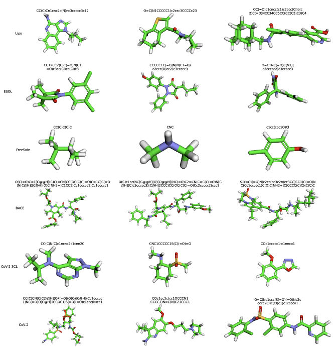
| Dataset | Conformers | GT and ConAN-FGW | GT and FGW-Mixup | ||||||
|---|---|---|---|---|---|---|---|---|---|
| N-Frobenius | MAE | MAPE | MSE | N-Frobenius | MAE | MAPE | MSE | ||
| FreeSolv | 3 | 0.1325 | 0.1727 | 0.3523 | 0.0812 | 0.1190 | 0.1590 | 0.3210 | 0.0671 |
| 5 | 0.1387 | 0.1823 | 0.3753 | 0.0870 | 0.1258 | 0.1695 | 0.3466 | 0.0731 | |
| 10 | 0.1431 | 0.1874 | 0.3876 | 0.0919 | 0.1323 | 0.1776 | 0.3638 | 0.0792 | |
| 15 | 0.1460 | 0.1924 | 0.3980 | 0.0947 | 0.1358 | 0.1819 | 0.3703 | 0.0832 | |
| 20 | 0.1453 | 0.1920 | 0.3954 | 0.0952 | 0.1336 | 0.1805 | 0.3662 | 0.0816 | |
| CoV-2 3CL | 3 | 0.0859 | 0.1696 | 0.4207 | 0.0670 | 0.0804 | 0.1626 | 0.4055 | 0.0600 |
| 5 | 0.0842 | 0.1688 | 0.4114 | 0.0632 | 0.0793 | 0.1616 | 0.3942 | 0.0569 | |
| 10 | 0.0879 | 0.1801 | 0.4452 | 0.0719 | 0.0806 | 0.1697 | 0.4201 | 0.0637 | |
| 15 | 0.0859 | 0.1729 | 0.4251 | 0.0670 | 0.0764 | 0.1571 | 0.3899 | 0.0543 | |
| 20 | 0.0902 | 0.1823 | 0.4558 | 0.0714 | 0.0865 | 0.1779 | 0.4460 | 0.0653 | |
D.6 Visualize Conformers Generated by RDKit
We present in Figure 7 typical 3D conformers generated by RDKit with their string inputs denote below each figure.