Structural sensitivity in the functional responses of predator-prey models
Abstract
In mathematical modeling, several different functional forms can often be used to fit a data set equally well, especially if the data is sparse. In such cases, these mathematically different but similar looking functional forms are typically considered interchangeable. Recent work, however, shows that similar functional responses may nonetheless result in significantly different bifurcation points for the Rosenzweig-MacArthur predator-prey system. Since the bifurcation behaviours include destabilising oscillations, predicting the occurrence of such behaviours is clearly important. Ecologically, different bifurcation behaviours mean that different predictions may be obtained from the models. These predictions can range from stable coexistence to the extinction of both species, so obtaining more accurate predictions is also clearly important for conservationists. Mathematically, this difference in bifurcation structure given similar functional responses is called structural sensitivity. We extend the existing work to find that the Leslie-Gower-May predator-prey system is also structurally sensitive to the functional response. Using the Rosenzweig-MacArthur and Leslie-Gower-May models, we then aim to determine if there is some way to obtain a functional description of data so that different functional responses yield the same bifurcation structure, i.e., we aim to describe data such that our model is not structurally sensitive. We first add stochasticity to the functional responses and find that better similarity of the resulting bifurcation structures is achieved. Then, we analyze the functional responses using two different methods to determine which part of each function contributes most to the observed bifurcation behaviour. We find that prey densities around the coexistence steady state are most important in defining the functional response. Lastly, we propose a procedure for ecologists and mathematical modelers to increase the accuracy of model predictions in predator-prey systems.
Department of Computer Science, Mathematics, Physics and Statistics, Irving K. Barber Faculty of Science, University of British Columbia Okanagan, SCI354, 1177 Research Road, Kelowna V1V 1V7, BC, Canada
Department of Mathematics and Statistics, Memorial University of Newfoundland, 230 Elizabeth Ave, St. John’s, A1C 5S7, NL, Canada
Department of Math, Physics, and Computer Science, University of the Philippines Mindanao, Mintal, Davao City, Philippines
⋆ Corresponding author.
Email addresses: [email protected] (S.K. Wyse), [email protected] (M.M. Martignoni),
[email protected] (M.A. Mata), [email protected] (E. Foxall), [email protected] (R.C. Tyson).
ORCID IDs: 0000-0002-5500-2711 (S.K. Wyse), 0000-0002-0192-8228 (M.M. Martignoni), 0000-0002-2967-344X (M.A. Mata), 0000-0003-1610-6662 (E. Foxall), 0000-0002-7373-4473 (R.C. Tyson).
Keywords – Structural sensitivity, bifurcation structure, functional response, coexistence steady state, stochasticity, prey density domain
Funding: This work was supported by The University of British Columbia Okanagan [Undergraduate Research Award] and Natural Sciences and Engineering Research Council of Canada [grant numbers RGPIN-2016-0577, RGPIN-2018-04480]. The funding sources were not involved in the conduction of research or preparation of this article.
1 Introduction
Mathematical modeling of biological phenomena necessitates making assumptions about the biological system so that the underlying mechanisms can be expressed mathematically. Indeed, the modeler must decide which features of a system to include and how to realistically formulate them (Krkošek et al., 2007; Barclay, 2001; Molnár et al., 2014; Cook et al., 1995; Baumgaertner et al., 2016; Majmudar et al., 2020). This process becomes more complicated when there are many apparently equivalent mathematical functions that may be used (Fussmann and Blasius, 2005). In this paper, we are interested in systems where the data is typically sparse and/or noisy, making it impossible to select one best-fitting functional curve (O’Donoghue et al., 2001). We focus here on the case of predator-prey systems and, in particular, on the predation interaction. The mathematical expression of this interaction is often referred to as the functional response.
A common assumption in modeling is that, if mathematical functions possess similar features and are appropriately parametrized to resemble one another, then the models utilizing these functional responses will produce essentially the same behaviour. Hence, many mathematicians typically choose a convenient functional response that fits the predation data. It was found, however, that similar looking functional responses may produce very different results (Fussmann and Blasius, 2005). Indeed, Fussmann and Blasius (2005) found that, for a given prey density, their model can produce high amplitude oscillations, bistability, or stable coexistence at low densities, depending on the form of the functional response, even if these responses are visually indistinguishable. This difference in model behaviour means that the assumption that similar curves can be used interchangeably does not always hold. This behaviour is called structural sensitivity. A structurally sensitive model has the property that a small perturbation in model functions, here the functional response, can lead to a different bifurcation structure. Ecologically, predictions made using models with different bifurcation structures could range from stable coexistence to extinction of both species.
The predator-prey system in Fussmann and Blasius (2005) is a Rosenzweig-MacArthur model that makes use of three similar functional response curves that are visually indistinguishable with respect to data fitting. The three functional responses are: Holling Type II, which is derived by considering how the predator’s activity is split between searching for and handling prey; Ivlev, which is based on the maximum digestion rate of the predator; and a hyperbolic tangent (trigonometric), which is a phenomenological curve that has no biological basis but is used in some population models (Aldebert et al., 2018). Although the theory behind each of these functional responses is different, they are considered interchangeable because it is difficult to determine if a predator is limited by its handling time or its digestion time. Jeschke et al. (2002) have developed a model that includes both of these limitations on predation together but we do not consider it in this manuscript. These functional responses have five specific characteristics in common: zero predation at zero prey density, monotonically increasing predation with increasing prey density, a negative second derivative, saturating behaviour at high prey density, and smoothness (Fussmann and Blasius, 2005; Seo and Wolkowicz, 2018).
Fussmann and Blasius (2005) found that the Rosenzweig-MacArthur model with these three functional response curves is structurally sensitive. That is, using the carrying capacity as the bifurcation parameter, this model produces different bifurcation diagrams for all three very similar looking functional responses. The model has a Hopf bifurcation of the coexistence steady state for all three functional response curves, but the critical value of the carrying capacity at which the Hopf bifurcation occurs varies by as much as 2000% from the smallest to largest critical transition value. For large values of the carrying capacity, the model that uses the Holling functional response produces large oscillations with limit cycles that approach very close to the prey-only and extinction steady states. On the other hand, the model using the trigonometric functional response initially produces smaller oscillations with limit cycles further from the prey-only and extinction steady states. The model using the Ivlev functional response produces oscillations of intermediate size. Additionally, the trigonometric model is the only model that has bistability. The difference in these results is problematic because the model disagreements make it impossible to determine, for example, if a real system is nearing a critical transition, such as the rapid emergence of large oscillations or extinction (Scheffer et al., 2009). This dilemma leads us to ask if there is a better way to mathematically describe data such that there is better similarity of the bifurcation structures obtained from different functional responses with respect to the bifurcation points, the coexistence steady state, and the branches of the limit cycles.
In recent literature, Adamson and Morozov (2014, 2013) have shown the existence of structural sensitivity in a range of mathematical models and have developed a test to determine whether or not a model is structurally sensitive. This test, however, does not address the question of how to alter the functional responses in a model to reduce or remove structural sensitivity, it only suggests that care must be taken in interpreting model predictions.
In this paper, we investigate three different approaches for translating a description of the data into a functional response curve. Our goal is to determine if any of our approaches can decrease or even remove structural sensitivity. First, we repeat the work of Fussmann and Blasius (2005) on another predator-prey model, the Leslie-Gower-May model, and find that it is also structurally sensitive to its functional response. We then base our study of structural sensitivity on the behaviour of these two different predator-prey models. Next, we study the effect of stochasticity of various types and amplitudes on the system and observe the resulting changes in structural sensitivity. Lastly, we investigate what part(s) of the functional response might be related to structural sensitivity.
In Section 2, we introduce the models and functional responses. In Section 3, we explain the methods we use to investigate structural sensitivity in the functional response. In Section 4, we state our results. In Section 5, we discuss and relate our findings to previous work and suggest a method to improve predictions obtained from structurally sensitive models.
2 Models
In this paper, we consider two classic predator-prey models: the Rosenzweig-MacArthur model and the Leslie-Gower-May model.
In the Rosenzweig-MacArthur model, prey density, , grows via logistic growth with a growth rate and carrying capacity . Predators and prey interact via a predation term, , which is discussed in more detail below. Lastly, predator density, , increases through growth related to predation and decreases through natural death with mortality rate . The Rosenzweig-MacArthur model is written (Turchin, 2013):
| (1a) | ||||
| (1b) | ||||
The parameter values given in Fussmann and Blasius (2005) are used throughout this paper (for the Rosenzweig-MacArthur model) unless specified otherwise.
The prey density equation in the Leslie-Gower-May model is the same as that in the Rosenzweig-MacArthur model. The predator density equation, on the other hand, has logistic growth of the predator with a growth rate and carrying capacity that decreases as prey density decreases. Here, the parameter is the equilibrium density ratio (Turhcin and Hanski, 1997). The Leslie-Gower-May model is written (Turchin, 2013):
| (2a) | ||||
| (2b) | ||||
The parameter values given in Vitense et al. (2016) are used throughout this paper (for the Leslie-Gower-May model) unless specified otherwise.
The predation functional response, , is our main focus. Following Fussmann and Blasius (2005), we consider the following three functional responses: Holling, Ivlev, and trigonometric. These functional responses are described, respectively, by the following three functions:
| (3a) | ||||
| (3b) | ||||
| (3c) | ||||
where and are the two parameters through which the curves can be fit to data, or to each other. The Rosenzweig-MacArthur functional responses have units of prey/predator/day and the Leslie-Gower-May functional responses have units of prey/predator/year. Note that in application, the three functional responses fit data equally well. Further, since each functional response has two parameters, it is not possible to distinguish the models using criteria such as the Akaike Information Criteria or Schwarz/Bayesian Information Criteria as these criteria rely greatly on the number of parameters used in each functional response (Akaike, 1974).
3 Methods
Structural sensitivity has not previously been established in the Leslie-Gower-May model. In this paper, we first show that model (2) is structurally sensitive. Then we study the structural sensitivity of the Rosenzweig-MacArthur and Leslie-Gower-May models by altering the functional responses (3) in the following three ways:
-
1.
Adding various types of stochasticity (Section 3.2).
-
2.
Varying the parameters and to fit the functional responses over a specified subset of the prey density domain (Section 3.3).
-
3.
Using continuous curves defined piecewise from two functional responses, switching from one to the other at a point where the functional response curves intersect (Section 3.4).
Method 1 uses stochasticity to create more overlap in the functional responses and hypothesizes that if the functional responses are more similar, then the resulting model behaviours will also become more similar. Methods 2 and 3 consist of focusing on different intervals of prey densities by applying a different weight to each part of the functional response. Our goal with these methods is to determine if there is a portion of the functional response that dictates the bifurcation structure.
Before investigating these methods to determine if we can decrease or remove structural sensitivity, we first fit our functional responses. To do this fitting, one of the functional responses is fixed and the other two are fit to the first response via nonlinear least squares to solve for the unknown and values. We use the Nelder-Mead algorithm (Nelder and Mead, 1965) to apply nonlinear least squares and chose the interval of prey densities to be [0,4] to match the previous work by Fussmann and Blasius (2005).
In the case of the Rosenzweig-MacArthur model, the fixed functional response is the Ivlev response and we fit the Holling and trigonometric functional responses to the fixed Ivlev functional response. As expected, we recover the same parameter values reported in Fussmann and Blasius (2005). In the case of the Leslie-Gower-May model, we use parameter values from Vitense et al. (2016) to define and fix the Holling functional response. Then, we fit the Ivlev and trigonometric functional responses to the fixed Holling functional response. The resulting Rosenzweig-MacArthur and Leslie-Gower-May functional responses appear in Figures S1a and 1(a).


| Rosenzweig-MacArthur | Leslie-Gower-May | |||||
|---|---|---|---|---|---|---|
| Holling | Ivlev | Trigonometric | Holling | Ivlev | Trigonometric | |
| 3.05 | 1 | 0.99 | 1683.333 | 451.447 | 446.182 | |
| 2.68 | 2 | 1.48 | 3.333 | 2.313 | 1.743 | |
3.1 Structural Sensitivity
To determine if the Leslie-Gower-May model is structurally sensitive, we plot a bifurcation diagram (shown in Figure 3(a)) using the carrying capacity , K, as the bifurcation parameter for each of the sub-models produced using the three functional responses (3) in model (2), and note the differences and similarities between them.
We find that the Leslie-Gower-May model is structurally sensitive: the Hopf bifurcation occurs at a very different carrying capacity for each sub-model. Figure 3(a) shows that the coexistence steady state in the model using the Holling functional response destabilizes at , in the Ivlev model at , and in the trigonometric model at . Additionally, the Ivlev and trigonometric models have saddle node bifurcations of limit cycles at and , respectively, and this bifurcation is not present in the Holling model. Following the formation of these limit cycles, bistability is observed in the Ivlev and trigonometric models. The Ivlev model is bistable over prey density values and the trigonometric model is bistable over prey density values .
3.2 Stochastic Model Methods
The addition of stochasticity to the functional responses makes them more like real data and increases their overlap. We add stochasticity to models (1) and (2) by rewriting the model equations in the following form:
| (4a) | ||||
| (4b) | ||||
| (4c) | ||||
i.e., is an Ornstein-Uhlenbeck process and solves a system of ODEs driven by . We use to alter the amount of noise included in each time step. is the right-hand-side of equations 1a and 2a (depending on the model in question) with in place of . Similarly, is the right-hand-side of equation 1b with in place of . Note that does not appear in equation 2b, so it is unchanged. Hence, model 4 is a system of one stochastic differential equation (SDE) and two ordinary differential equations (ODEs). At each time step, we sample a Gaussian random variable, where , and solve the SDE (equation 4a) using the Euler-Maruyama scheme to obtain . Then, we plug into the system of ODEs and numerically solve the system using Euler’s method with a step size small enough to achieve stable solutions. Note that if the solutions result in prey or predator densities less than zero due to the stochastic element, then the prey or predator density is set to zero. For the Rosenzweig-MacArthur model, we use and for the Leslie-Gower-May model, we use unless specified otherwise. Sample stochastic functional responses are given in Figures 1(b) and S1b. The corresponding results are given in Section 4.1.
3.3 Fitted Functional Response Methods
The behaviour of both the Rosenzweig-MacArthur and the Leslie-Gower-May models is stable coexistence for values of the carrying capacity, , less than the destabilizing bifurcation. We hypothesize that if the model behaviour is more similar leading up to the destabilizing bifurcation, then perhaps the destabilizing bifurcation will occur for more similar values of the carrying capacity. If our hypothesis is correct, it suggests that a key portion of the functional response is in the vicinity of the coexistence steady state.
We choose an interval containing the prey density values of the coexistence steady state to perform the fit. We call this interval the fitting region and choose it such that it is smaller than the original fitting region. Note that we choose this region regardless of whether the coexistence steady state is stable or unstable. In models that do not use data, we choose a functional response to be fixed. We will refer to the sub-model where Holling is chosen as the fixed functional response as the fixed Holling case and the other sub-models follow the same naming scheme. Note that in the applied case of this method, we do not have to choose a fixed functional response since we can fit the functional responses to data. We then apply nonlinear least squares to the functional responses fit to either the fixed functional response or to data over the fitting region. The average prey density values of the coexistence steady states in the Rosenzweig-MacArthur and Leslie-Gower-May models are and , respectively. So, the corresponding fitting regions are taken to be and . The parameter values obtained from this fit to the fixed Holling functional response are given in Table 2. The fixed Ivlev and fixed trigonometric functional responses are given in Figures S1c and S4. The corresponding parameter values are given in Table S1. The Holling fitted functional response results are given in Section 4.2.
| Rosenzweig-MacArthur | Leslie-Gower-May | |||||
|---|---|---|---|---|---|---|
| Holling | Ivlev | Trigonometric | Holling | Ivlev | Trigonometric | |
| 3.05 | 0.6282 | 0.3707 | 1683.333 | 399.8009 | 384.1465 | |
| 2.68 | 4.8204 | 7.6281 | 3.333 | 3.1656 | 2.4028 | |
3.4 Piecewise Identical Functional Response Methods
Here, rather than fitting the functional responses to each other, we modify the functional responses so that they are exactly the same over portions of the prey density domain . Each functional response has three intersection points with each of the other two functional responses. All three functional responses intersect at (0,0), since there is zero predation at zero prey density. The values for the non-trivial intersections of the Rosenzweig-MacArthur and the Leslie-Gower-May functional response are given in Table 3. As a result, we can consider piecewise functional responses made up of contributions from two functional responses. These piecewise functional responses give us another way to ask if there is a key part of the functional response that determines the model behaviour. That is, we can examine how each portion of the functional response, (i.e., low, medium, and high prey density) affects the model’s bifurcation structure.
We consider three cases for each functional response for each model (18 cases total). To form each case we choose two functional responses and interchange the functional response we use for each of the three regions. The intersections noted earlier become the transition points between the regions. Sample piecewise functional responses are given in Figures 1(d) and S1d. In these figures, we introduce notation that is used from here forward to describe the piecewise identical sub-models. This notation is a three letter code that corresponds to each of the three prey density regions we have chosen to investigate, with Holling, Ivlev, and trigonometric functions each represented by their first letter. For example, HII represents the functional response that uses the Holling functional response for low prey densities, and uses the Ivlev functional response for medium and high prey densities. The corresponding results are given in Section 4.3.
| Rosenzweig-MacArthur | Holling/Ivlev | Ivlev/Trig | Trig/Holling |
|---|---|---|---|
| Extinction | 0 | 0 | 0 |
| Low to medium prey density | 0.6191 | 0.5651 | 0.5942 |
| Medium to high prey density | 2.5799 | 2.1597 | 2.4695 |
| Leslie-Gower-May | Holling/Ivlev | Ivlev/Trig | Trig/Holling |
| Extinction | 0 | 0 | 0 |
| Low to medium prey density | 0.5726 | 0.4458 | 0.5152 |
| Medium to high prey density | 2.4486 | 2.2611 | 1.8077 |
4 Results
4.1 Stochastic Model Results
In the case of the Rosenzweig-MacArthur model, we added Gaussian stochasticity with . We choose this amplitude because stochasticity of smaller amplitude had virtually no effect on the bifurcation structure. stochasticity adds some variance to the time series but does not significantly alter the qualitative behaviour for carrying capacities less than the Hopf bifurcation in the deterministic model. That is, given initial conditions that lead to the stable coexistence steady state in the deterministic case, the stochastic model also results in trajectories that converge to the coexistence steady state. For values of the carrying capacity greater than that of the bifurcation in the deterministic model, the lower side of the limit cycle reaches very low prey densities of approximately at times ( times smaller than the stochasticity). As a result, the stochasticity causes extinction within 100 time steps in most of the time series of the stochastic model for carrying capacities greater than that of the deterministic model’s destabilizing bifurcation. These results mean that we are unable to clearly observe the stochastic behaviour and we cannot conclude whether or not stochasticity reduces structural sensitivity in the Rosenzweig-MacArthur model.
In the case of the Leslie-Gower-May model, we added Gaussian stochasticity with . As in the case of the Rosenzweig-MacArthur model, we chose this amplitude of stochasticity because it is large enough to affect the bifurcation structure, but not so large that all of trajectories rapidly terminate in extinction of the predator or both populations. Results obtained from both smaller and larger amplitudes of stochasticity are provided in the Supplementary Material (Figure S3).
The bifurcation diagrams (quasi-steady state behaviour) for the stochastic Leslie-Gower-May model are given in Figure 3(b). This figure shows better similarity in the bifurcation structures with the addition of stochasticity. The bifurcation structures are obtained by plotting the maximum and minimum of the stochastic time series (after removal of transients). Thus, these windows show the smallest value of the carrying capacity for which the coexistence steady states may destabilize. Limit cycles in our stochastic model appear to have greater amplitude than those of the deterministic model. We find that the stochastic bifurcation structures show better similarity than the deterministic model’s bifurcation structures. This similarity suggests that there is a decrease in structural sensitivity of the model.
Plots of time series (Figure S2) indicate that bistability remains a property of the stochastic Ivlev and trigonometric models. In the bistable regions, the solution trajectories of the Ivlev and trigonometric models alternate randomly between the coexistence steady state and the stable limit cycle, and also spend some time at the unstable limit cycle. This ability to alternate between stable and unstable steady states is unique to the stochastic model, and has been observed in other work (Sharma et al., 2015; Abbott and Nolting, 2017). These observations occur for small to intermediate stochastic amplitudes, larger amplitudes lead to rapid extinction, and more generally, to the stochastic behaviour washing out the deterministic structure.


4.2 Fitted Functional Response Results
We only consider the fixed Holling case here as the fixed Ivlev and fixed trigonometric cases are similar and given in the Supplementary Material (Figures S4 and S5).
The Rosenzweig-MacArthur fitted functional response sub-models yield the bifurcation plots shown in Figure 2(b). The bifurcation values for these sub-models are given in Table 4. These fits result in better similarity of the bifurcation structures and less structural sensitivity as compared to the original model (Figure 2(a)). For example, when the Ivlev functional response is fit to the fixed Holling functional response, the Ivlev fit to Holling sub-model shows behaviour similar to the Holling only sub-model as there is a leftward shift in the destabilizing Hopf bifurcation. This result holds across each of the fits. Hence, considering the prey densities in the chosen fitting region appears to be a better metric to describe functional responses in the Rosenzweig-MacArthur model; in the sense that model behaviour is less sensitive to small changes in the functional response using this method.
The Leslie-Gower-May fitted functional response sub-models yield the bifurcation diagrams given in Figure 3(c) and the value of the bifurcation parameter for each bifurcation is given in Table 4. The resulting sub-models show better similarity in bifurcation structure when compared to the fixed functional response. For example, Ivlev fit to Holling shows a leftward shift of the Hopf bifurcation as compared to the Ivlev only bifurcation structure and the disappearance of the saddle bifurcation of limit cycles. So, the Ivlev fit to Holling sub-model shows behaviour similar to the Holling only sub-model. The same result holds for each of the other cases, and there is better similarity in model behaviour when compared to the fixed functional response. Therefore, as in the Rosenzweig-MacArthur model, fitting the functional responses over the chosen fitting region appears to decrease structural sensitivity in the Leslie-Gower-May model.
We would like to note that these theoretical results are subjective to which functional response is chosen to be fixed. That is, the model behaviour will always become more similar to the fixed model. In the case of the results shown in this section, the model behaviour always becomes more similar to the Holling sub-model behaviour. Our method when applied to a model that uses data to fit the functional responses, however, is not subjective. We will discuss this application of our method to data further in Section 5.2.
| Rosenzweig-MacArthur | Leslie-Gower-May | |||||
| Original Model (2(a), 3(a)) | Holling | Ivlev | Trig | Holling | Ivlev | Trig |
| Hopf | 0.4452 | 1.071 | 10.12 | 5.554 | 12.09 | 26.36 |
| Limit Cycle Saddle | - | - | 2.644 | - | 10.51 | 12.94 |
| Holling Fixed (2(b), 3(c)) | Holling | Ivlev | Trig | Holling | Ivlev | Trig |
| Hopf | 0.4452 | 0.4632 | 0.7729 | 5.554 | 5.857 | 6.052 |
| Limit Cycle Saddle | - | - | 0.5057 | - | - | 5.964 |
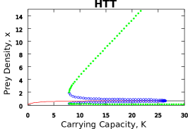
| Pw-I Holling (2(c), 3(d)) | HTT | THT | HHT | HTT | THT | HHT |
| Hopf | 0.4451 | 0.4451 | 0.4451 | 26.36 | 26.36 | 5.554 |
| Limit Cycle Saddle | - | - | - | 7.95 | 7.95 | - |
| Pw-I Trigonometric (2(c), S8) | THH | HTH | TTH | THH | HTH | TTH |
| Hopf | 10.12 | 10.12 | 10.12 | 5.554 | 5.554 | 26.36 |
| Limit Cycle Saddle | 2.431 | 2.431 | 2.644 | - | - | 13.13 |
4.3 Piecewise Identical Functional Response Results
Suppose that medium prey densities determine the bifurcation structure of a model. Then, according to our hypothesis, we expect YXY and ZXZ to show model behaviours more similar to the X model behaviour (be that H, I, or T). Based on the results in Section 4.2, we might actually expect low prey densities to be the most important, in which case we expect XYY and XZZ to have better similarity to the X model behaviour. However, our results show that none of the three regions we consider separately determine the model behaviour. In this section, we describe only the piecewise identical functional responses made up of the Holling and trigonometric functional responses. The bifurcation diagrams for these cases of the Rosenzweig-MacArthur and Leslie-Gower-May sub-models are given in Figures 2(c) and 3(d). The rest of the cases are similar and are given in the Supplementary Material (Figures S6-S8).
In the case of the Rosenzweig-MacArthur model, there is not better similarity of the Holling to trigonometric sub-models (i.e., sub-models of the form HTT, THT, or HHT) behaviour towards the trigonometric behaviour. This result suggests that both the first and second regions determine the resulting bifurcation behaviour of the Rosenzweig-MacArthur model and that these regions are the most structurally sensitive.
However, the Rosenzweig-MacArthur trigonometric to Holling piecewise identical sub-models (i.e., sub-models of the form THH, HTH, or TTH) are slightly different. In the THH plot, there is a small leftward shift of the saddle bifurcation of limit cycles from the original value (Table 4) at to . There is, however, no change in the location of the Hopf bifurcation. In the HTH plot, the same leftward shift occurs. Lastly, the TTH plot has a resulting bifurcation structure that matches that of the trigonometric only functional response model behaviour. Overall, the trigonometric functional response has a strong effect on the bifurcation structure. Further, when the Holling functional response takes up two of the three regions (in the THH and HTH cases), the Holling functional response has an effect, though limited, on the bifurcation structure. This effect causes the aforementioned shift in the saddle bifurcation of limit cycles. The piecewise identical functional responses seem to affect the resulting model behaviour without following any clear rules. Hence, we are unable to make any claims on which prey density regions determine the Rosenzweig-MacArthur model behaviour.
In the case of the Leslie-Gower-May model, the HTT and THT sub-models show better similarity when compared to the trigonometric bifurcation structure while the resulting bifurcation structure for the HHT sub-model matches that of the Holling only functional response. We found that in the Leslie-Gower-May model, the functional response that is used across more prey density regions is the one that determines where the Hopf bifurcation occurs and whether there exists a saddle bifurcation of limit cycles. However, the functional response used across only one prey density region causes a shift in the saddle bifurcation of limit cycles (if it exists) for every case, except surprisingly the IIH sub-model where there is no shift from the Ivlev behaviour (Figure S8). This result means that the sub-models with the Holling functional response describing two prey density regions result in only Holling model behaviour, but the sub-models with either the Ivlev or trigonometric functional response describing two prey density regions result in mixed dynamics.
5 Discussion
5.1 Reducing Structural Sensitivity
Structural sensitivity is an intrinsic feature of a wide range of ecological models (Adamson and Morozov, 2013, 2014). In our work, we focus on predator-prey models and investigate the structural sensitivity that occurs with respect to the predation function. Our work has attempted to answer how to fit data in such a way to gain confidence in the results, regardless of which curve is used. We found that only the sub-models that use the functional responses fit around the coexistence steady state consistently decrease structural sensitivity across both the Rosenzweig-MacArthur and Leslie-Gower-May models. Using this result, we also give suggestions as to which intervals of prey density are most relevant when fitting a functional response to data and which intervals of prey density are most relevant for ecologists to collect data.
5.1.1 Stochasticity
One of the differences between the functional response curves in Fussmann and Blasius (2005) and real data is that the latter include stochasticity. A model’s steady states and deterministic structure only provide a partial understanding of the stochastic structure and so the stochastic system may behave in unanticipated ways (Sharma et al., 2015). Hence, it is important to consider a stochastic model when analyzing biological systems. We examine the effect of adding stochasticity to the functional responses of the Rosenzweig-MacArthur and Leslie-Gower-May models and, specifically, whether or not this addition can remove or decrease structural sensitivity.
In our work, we observe that the destabilizing of the coexistence steady state can occur earlier in the stochastic system than the deterministic system. Most notably, there is greater similarity in the stochastic bifurcation structures from the three functional responses implying decreased structural sensitivity. We find that the maximum and minimum values of the deterministic system lie within the interval determined by the maximum and minimum values of the stochastic system. This result supports the observation that trajectories in the stochastic system may approach the steady states of the deterministic system (Aguirre et al., 2013; Predescu et al., 2007). How stochasticity alters a model’s behaviour from the deterministic system depends on the amplitude and distribution of the stochastic random variable. For example, white noise weakens bistable behaviour while red noise can amplify the bistability observed in a system (Sharma et al., 2015). Using a different distribution can change the shape and depth of potential wells, and thus produce different stability properties (Sharma et al., 2015). We do not, however, study other stochastic distributions here and leave this investigation for future work.
White noise is widely used in studies of stochastic models (van der Bolt et al., 2018). It is characterized by having the same variance at all frequencies. However, in recent years, there has been interest in varying the colour, or auto-correlation, of applied noise. Red noise, which has more auto-correlation and is characterized by low frequencies, has been found to better describe the stochasticity found in ecological systems (Vasseur and Yodzis, 2004; Greenman and Benton, 2003; Grove et al., 2020; Jonsson and Wennergren, 2019). In this paper, we only consider white noise. An interesting future step is to consider the effect of red noise on the bifurcation structure of the stochastic system.
5.1.2 Fitted Functional Responses
It is sometimes possible to improve mathematical model predictions through describing data in a particular way. In order to help ecologists make accurate decisions regarding conservation efforts, it is important to obtain the best model predictions possible. We discuss the use of data in these model predictions further in Section 5.2 below.
In our models, the slopes of the functional response curves are greatest near the coexistence steady state, meaning that this region is also where the predator response to a change in prey density is strongest (Aldebert et al., 2016). This property suggests that having a higher density of data points in the region of the functional response domain near the coexistence steady state prey density value, or giving these data points more weight, is important. Further, since the initial behaviour of all three models is similar and all are stable at the coexistence steady state before any destabilizing occurs, we hypothesized that if the corresponding part of the functional response (region around the stable or unstable coexistence steady state prey density value) held more weight in the nonlinear least squares fitting, then the bifurcation structures would be more similar. That is, if the fitted functional responses method (Section 3.3) is a better metric to decrease structural sensitivity, we expect to observe better similarity of the resulting model’s bifurcation structure. We found that this hypothesis is supported in both the Rosenzweig-MacArthur and the Leslie-Gower-May models.
5.1.3 Piecewise Identical Functional Responses
We found that more similar bifurcation structures are obtained for functional responses that fit very closely at low and intermediate prey density values, but also disagree wildly at large prey density values near saturation. So, the piecewise identical functional response results suggest that low and medium prey densities are the most important regions to fit to decrease structural sensitivity.
Our results, however, appear to be in contrast from previous findings, indicating that it is most important to have data at saturation or high prey densities (Aldebert and Stouffer, 2018). However, this contradiction is only apparent. In our work, we attempt to decrease structural sensitivity and describe the functional responses such that any of the three can be used to provide equally accurate predictions. On the other hand, Aldebert and Stouffer (2018) aim to choose one functional response that fits the model best. To do so, they suggest collecting data around saturation such that the functional responses result in models with vastly different bifurcation structures. Since structural sensitivity in the resulting models is increased, it becomes easier to determine which functional response and model fit the data best. While the authors are able to choose a best functional response to fit data, the model remains structurally sensitive.
5.2 Using Data in Models
The main application of our work is in models that use data to fit the functional response. As we noted in Section 4.2, the choice of the fitted functional response is subjective if our method is used merely theoretically. However, in the case of applied models, our method is no longer subjective since we fit the functional responses to data instead of a subjectively chosen fixed functional response. Once all three functional responses are fit using our method to make their bifurcations structures more similar, the resulting bifurcation structure should show the behaviour of the data rather than a single chosen functional response.
Ecological data, however, is typically sparse as it is often difficult to collect (Ovaskainen and Soininen, 2011). Furthermore, the data is also typically very noisy. As a result, it is important that ecologists know what data is most important to collect to build accurate models that can be used with confidence to predict future population dynamics. In Section 4.2, we found that model predictions are most consistent if the functional responses match over the coexistence steady state prey density region. The implication is that better predictions can be obtained if there is additional data near the coexistence steady state. We believe that this region of prey densities is most important in fitting the functional responses because it corresponds to the steady state behaviour for values of the carrying capacity less than destabilizing bifurcation. The idea being that if the model behaviour is more similar before the destabilizing bifurcation, then the destabilizing bifurcation may occur for more similar values of the carrying capacity. This result opposes previous work that states saturation is the most important part to match of the functional responses (Aldebert and Stouffer, 2018).
To apply our result to ecological data and to make predictions in predator-prey models, we propose the following procedure:
-
1.
Collect data as per normal methods,
-
2.
Fit the three functional responses to this data and determine the parameter values for each and ,
-
3.
Use the functional responses to choose a fitting region around the stable or unstable coexistence steady state prey density values across all three models,
-
4.
Do one or both of the following:
-
(a)
Collect more data for prey densities in the coexistence steady state prey density region,
-
(b)
Give more weight to the data in the coexistence steady state prey density region,
-
(a)
-
5.
Fit the three functional responses again and use these functional responses to make predictions regarding the system.
This algorithm takes into account our result that collecting data for prey densities around the coexistence steady state appears to be most important while also considering the difficulty of collecting data (step 4b). Note that we have only considered structural sensitivity with respect to the functional response in this work. Models that are structurally sensitive with respect to other terms, such as prey growth, may require a different algorithm.
6 Conclusion
Structural sensitivity in the functional response of a model can cause similar functional responses to produce very different bifurcation structures. In this paper, we investigated three potential methods to achieve better similarity of resulting bifurcation structures. We found that 1) stochasticity results in better similarity of the bifurcation structures, 2) functional responses fit over the coexistence steady state prey density region seem to decrease structural sensitivity, and 3) piecewise identical functional responses do not consistently decrease structural sensitivity. Overall, adding stochasticity and fitting functional responses over the coexistence steady state prey density region appear to reduce structural sensitivity. Further investigation into the fitted functional response method is necessary to determine if there is an optimal interval size that decreases structural sensitivity the most.
Investigating other types of stochasticity, specifically red noise or noise with stronger auto-correlation, remains an interesting question for further investigation. Working with ecological data to test our proposed procedure and make predictions regarding the population dynamics of a predator-prey system is a very useful application of this work. It is also of interest to investigate more predator-prey models and more functional response curves to determine if our results generalize. It is also possible to have structural sensitivity occur with respect to the prey growth function (Adamson and Morozov, 2013). This type of structural sensitivity remains an area for future investigation.
As part of this work, we also investigated the derivatives of the functional responses. That is, we fit the parameters and such that the derivatives of the functional responses were as similar as possible. This method of fitting did not show promise and requires further investigation to determine if it can decrease structural sensitivity.
References
- Abbott and Nolting (2017) Abbott, K.C., Nolting, B.C.: Alternative (un)stable states in a stochastic predator–prey model. Ecol. Complex. 32, 181–195 (2017). DOI 10.1016/j.ecocom.2016.11.004
- Adamson and Morozov (2013) Adamson, M.W., Morozov, A.Y.: When can we trust our model predictions? unearthing structural sensitivity in biological systems. Proc. Math. Phys. Eng. Sci. 469(2149) (2013). DOI 10.1098/rspa.2012.0500
- Adamson and Morozov (2014) Adamson, M.W., Morozov, A.Y.: Defining and detecting structural sensitivity in biological models: developing a new framework. J. Math. Biol. 69, 1815–1848 (2014). DOI 10.1007/s00285-014-0753-3
- Aguirre et al. (2013) Aguirre, P., González-Olivares, E., Torres, S.: Stochastic predator–prey model with allee effect on prey. Nonlinear Anal. Real World Appl. 14(1), 768–779 (2013). DOI 10.1016/j.nonrwa.2012.07.032
- Akaike (1974) Akaike, H.: A new look at the statistical model identification. IEEE Trans. Automat. Contr. 19(6), 716–723 (1974). DOI 10.1109/tac.1974.1100705
- Aldebert et al. (2018) Aldebert, C., Kooi, B.W., Nerini, D., Poggiale, J.C.: Is structural sensitivity a problem of oversimplified biological models? insights from nested dynamic energy budget models. J. Theor. Biol. 448, 1–8 (2018). DOI 10.1016/j.jtbi.2018.03.019
- Aldebert et al. (2016) Aldebert, C., Nerini, D., Guaduchon, M., Poggiale, J.C.: Structural sensitivity and resilience in a predator-prey model with density-dependent mortality. Ecol. Complex. 28, 163–173 (2016). DOI 10.1016/j.ecocom.2016.05.004
- Aldebert and Stouffer (2018) Aldebert, C., Stouffer, D.B.: Community dynamics and sensitivity to model structure: towards a probabilistic view of process-based model predictions. J. R. Soc. Interface 15(149), 20180,741 (2018). DOI 10.1098/rsif.2018.0741
- Barclay (2001) Barclay, H.J.: Modeling incomplete sterility in a sterile release program: interactions with other factors. Popul. Ecol. 43, 197–206 (2001). DOI 10.1007/s10144-001-8183-7
- Baumgaertner et al. (2016) Baumgaertner, B.O., Tyson, R.C., Krone, S.M.: Opinion strength influences the spatial dynamics of opinion formation. J. Math. Sociol. 40(4), 207–218 (2016). DOI 10.1080/0022250X.2016.1205049
- Cook et al. (1995) Cook, J., Tyson, R., White, J., Rushe, R., Gottman, J., Murray, J.: Mathematics of marital conflict: Qualitative dynamic mathematical modeling of marital interaction. J. Fam. Psychol. 9(2), 110–130 (1995). DOI 10.1037/0893-3200.9.2.110
- Fussmann and Blasius (2005) Fussmann, G., Blasius, B.: Community response to enrichment is highly sensitive to model structure. Biol. Lett. 1(1), 9–12 (2005). DOI 10.1098/rsbl.2004.0246
- Greenman and Benton (2003) Greenman, J.V., Benton, T.G.: The amplification of environmental noise in population models: Causes and consequences. Am. Nat. 161(2), 225–239 (2003). DOI 10.1086/345784
- Grove et al. (2020) Grove, M., Borg, J.M., Polack, F.: Coloured noise time series as appropriate models for environmental variation in artificial evolutionary systems (2020). DOI 2006.16204
- Jeschke et al. (2002) Jeschke, J.M., Kopp, M., Tollrian, R.: Predator functional responses: Discriminating between handling and digesting prey. Ecol. Monogr. 72(1), 95–112 (2002). DOI 10.2307/3100087
- Jonsson and Wennergren (2019) Jonsson, A., Wennergren, U.: Approximations of population growth in a noisy environment: on the dichotomy of non-age and age structure. Theor. Ecol. 12, 99–110 (2019). DOI 10.1007/s12080-018-0391-2
- Krkošek et al. (2007) Krkošek, M., Ford, J.S., Morton, A., Lele, S., Myers, R.A., Lewis, M.A.: Declining wild salmon populations in relation to parasites from farm salmon. Science 318(5857), 1772–1775 (2007). DOI 10.1126/science.1148744
- Majmudar et al. (2020) Majmudar, J.R., Krone, S.M., Baumgaertner, B.O., Tyson, R.C.: Voter models and external influence. J. Math. Sociol. 44(1), 1–11 (2020). DOI 10.1080/0022250X.2019.1625349
- Molnár et al. (2014) Molnár, P.K., Lewis, M.A., Derocher, A.E.: Estimating allee dynamics before they can be observed: Polar bears as a case study. PLOS ONE 9(1), 1–12 (2014). DOI 10.1371/journal.pone.0085410
- Nelder and Mead (1965) Nelder, J.A., Mead, R.: A simplex method for function minimization. Comput. J. 7(4), 308–313 (1965). DOI 10.1093/comjnl/7.4.308
- O’Donoghue et al. (2001) O’Donoghue, M., Boutin, S., Murray, D.L., Krebs, C.J., Hofer, E.J., Breitenmoser, U., Christine Breitenmoser-Würsten, G.Z., Doyle, C., Nams, V.O.: Mammalian predators: Coyotes and lynx. In: Krebs, C.J., Boutin, S., Boonstra, R. (eds.) Ecosystem Dynamics of the Boreal Forest: The Kluane Project, 1 edn., chap. 13, pp. 275–323. OUP (2001)
- Ovaskainen and Soininen (2011) Ovaskainen, O., Soininen, J.: Making more out of sparse data: Hierarchical modeling of species communities. Ecology 92(2), 289–95 (2011). DOI 10.1890/10-1251.1
- Predescu et al. (2007) Predescu, M., Sirbu, G., Levins, R., Awerbuch-Friedlander, T.: On the dynamics of a deterministic and stochastic model for mosquito control. Appl. Math. Lett. 20(8), 919–925 (2007). DOI 10.1016/j.aml.2006.12.001
- Scheffer et al. (2009) Scheffer, M., Bascompte, J., Brock, W.A., Brovkin, V., Carpenter, S.R., Dakos, V., Held, H., van Nes Egbert, H., Rietkerk, M., Sugihara, G.: Early-warning signals for critical transitions. Nature 461(7260), 53–59 (2009). DOI 10.1038/nature08227
- Seo and Wolkowicz (2018) Seo, G., Wolkowicz, G.S.K.: Sensitivity of the dynamics of the general rosenzweig–macarthur model to the mathematical form of the functional response: a bifurcation theory approach. J. Math. Biol. 76, 1873–1906 (2018). DOI 10.1007/s00285-017-1201-y
- Sharma et al. (2015) Sharma, Y., Abbott, K.C., Dutta, P.S., Gupta, A.K.: Stochasticity and bistability in insect outbreak dynamics. Theor. Ecol. 8, 163–174 (2015). DOI 10.1007/s12080-014-0241-9
- Turchin (2013) Turchin, P.: Trophic interaction. In: Complex Population Dynamics, Monogr. Popul. Biol., chap. 4, pp. 95–100. PUP (2013)
- Turhcin and Hanski (1997) Turhcin, P., Hanski, I.: An empirically based model for latitudinal gradient in vole population dynamics. Am. Nat. 149, 842–874 (1997). DOI 10.1086/286027
- van der Bolt et al. (2018) van der Bolt, B., van Nes, E.H., Bathiany, S., Vollebregt, M.E., Scheffer, M.: Climate reddening increases the chance of critical transitions. Nat. Clim. Change. 8, 478–484 (2018). DOI 10.1038/s41558-018-0160-7
- Vasseur and Yodzis (2004) Vasseur, D., Yodzis, P.: The color of environmental noise. Ecology 85(4), 1146–1152 (2004). DOI 10.1890/02-3122
- Vitense et al. (2016) Vitense, K., Wirsing, A.J., Tyson, R.C., Anderson, J.J.: Theoretical impacts of habitat loss and generalist predation on predator–prey cycles. Ecol. Modell. 327, 85–94 (2016). DOI 10.1016/j.ecolmodel.2016.02.002