Strong and weak (1, 2) homotopies on knot projections and new invariants
Abstract.
Every second flat Reidemeister move of knot projections can be decomposed into two types thorough an inverse or direct self-tangency modification, respectively called strong or weak, when orientations of the knot projections are arbitrarily provided. Further, we introduce the notions of strong and weak (1, 2) homotopies; we define that two knot projections are strongly (resp. weakly) (1, 2) homotopic if and only if two knot projections are related by a finite sequence of first and strong (resp. weak) second flat Reidemeister moves. This paper gives a new necessary and sufficient condition that two knot projections are not strongly (1, 2) homotopic. Similarly, we obtain a new necessary and sufficient condition in the weak (1, 2) homotopy case. We also define a new integer-valued strong (1, 2) homotopy invariant. Using it, we show that the set of the non-trivial prime knot projections without -gons that can be trivialized under strong (1, 2) homotopy is disjoint from that of weak (1, 2) homotopy. We also investigate topological properties of the new invariant and give its generalization, a comparison of our invariants and Arnold invariants, and a table of invariants.
Key words and phrases:
knot projection; spherical curve; strong (1, 2) homotopy; weak (1, 2) homotopy; non-Seifert resolution1. Introduction
A knot projection is defined as the image of a generic immersion of a circle into a -dimensional sphere. Historically, the equivalence classes of knot projections generated by the first and second flat Reidemeister moves shown in Fig. 1 are determined by Khovanov [7, Theorem 2.2] via the notion of doodles, introduced by Fenn and Taylor [3, 2] (cf. [5, Theorem 2.2]). Essentially, by using (1, 2)-reduced knot projections, which are knot projections without any - or -gons, we can detect whether two given knot projections are equivalent under the equivalence relations obtained by the first and the second flat Reidemeister moves. Here, a -gon (resp. -gon) is the boundary of a disk with exactly one (resp. two) vertex and exactly one (resp. two) edges, where a knot projection consists of vertexes and edges (Fig. 1).
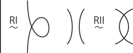
Nonetheless, to the best of our knowledge, there have still been two open problems: find a nice necessary and sufficient condition for two knot projections being equivalent under a given equivalence relation, called strong homotopy (resp. weak homotopy), consisting of the first flat Reidemeister moves denoted by RIs and the strong RIIs (resp. weak RIIs ) as defined by Fig. 2 (center) (resp. Fig. 2 (right)). The equivalence induced by RI is denoted by . The equivalence induced by strong RII (resp. weak RII) is denoted by (resp. ). The -gon appearing in a strong (resp. weak) RII is called a coherent ( resp. incoherent ) -gon if the -gon is (resp. is not) be oriented by orienting a knot projection.

In this paper, let (resp. ) be strong (resp. weak) (1, 2) homotopy and let be sphere isotopy (often simply called isotopy). The definition of the strong or weak RII is a natural notion as a second flat Reidemeister move (Fig. 1, right) is decomposed into just the two kinds of local moves shown in Fig. 2; one is strong RII, and the other is a weak RII. The strong (resp. weak) RII is also treated as the inverse (resp. direct) self-tangency perestroika as in Arnold [1] if the knot projections are oriented. In the rest of this paper, a knot projection having no double points is simply called a simple closed curve or a trivial knot projection.
The answers to the two aforementioned problems appear in this paper (Theorem 1), serving as the starting point.
Theorem 1.
Let a knot projection with no -gons and no incoherent (resp. coherent) -gons be called a weak (resp. strong) reduced knot projection (resp. ), only decreasing double points by any RIs or weak (resp. strong) RIIs from a knot projection .
and are weakly (1, 2) homotopic if and only if and are isotopic.
and are strongly (1, 2) homotopic if and only if and are isotopic.
Here, the next problem arises: how do the two equivalence relations, weak and strong (1, 2) homotopies, classify knot projections? This paper obtains a partial answer to that problem.
Theorem 2.
Let be a knot projection having no double points, namely a simple circle on the -sphere. Then a knot projection is strongly (1, 2) homotopic and weakly (1, 2) homotopic to if and only if and are transformed into each other by RIs and isotopies.
To prove Theorem 2, this paper introduces a topological invariant of knot projections obtained by applying the replacement shown in Fig. 3 at every double point. The replacements do not depend on an orientation of a knot projection and are denoted as “” in [4]. We call replacement , or non-Seifert resolution.

One may feel that this local replacement is similar to Seifert resolution (Fig. 4).

Seifert resolution has many crucial roles in the basics of today’s Knot Theory; for instance, genus, Alexander polynomial, or Khovanov-Lee homology. It also has an important role in the theory of generic immersed plane curves: e.g., it provides the Alexander numbering and Arnold invariants of plane curves [10, 8]. In these roles, one of the advantages of Seifert resolution is that it preserves the orientation of an oriented curve. In comparison, does not preserve the orientation if the curve is oriented, and thus one may think that would not have such an important role.
However, this paper shows that has nice properties and applications. One of the advantages of is that for a non-oriented curve, does not change under RI, while each Seifert resolution changes the number of components under RI. In fact, gives invariants of knot projections under both RI and strong RII as shown in Fig. 2.
For example, let us consider our familiar object, the chord diagram (often called Gauss diagram), which is one circle with finitely many chords where each chord connects the preimages of each double point of a knot projection. The number , introduced by [6], is defined as the number of sub-chords as “” embedded in the whole chord diagram of a given knot projection ; modulo is then an invariant under strong (1, 2) homotopy, though it is a -valued invariant.
An easily calculated -valued strong (1, 2) homotopy invariant, called circle number, is introduced in this paper using non-Seifert resolution . We also give a generalization of the -valued invariant, called circle arrangement, under strong (1, 2) homotopy and obtain its table of prime knot projections with small numbers of double points. We call these new invariants as a whole circle invariants.
This paper is constructed as follows. Sec. 2 proves Theorem 1. Sec. 3 defines a new -valued invariant, circle numbers, under strong (1, 2) homotopy and also gives a new, strictly stronger invariant, circle arrangements. Sec. 4 explores the characteristics of circle numbers. Sec. 5 proves Theorem 2. Sec. 6 explores the characteristics of circle arrangements. Finally, Sec. 7 obtains a table of prime knot projections with small numbers of double points including information on circle numbers and circle arrangements.
2. Proof of Theorem 1
We need two lemmas which are needed to prove Theorem 1.
Lemma 1.
A move RI increasing (resp. decreasing) double points is denoted by (resp. ). Weak RII increasing (resp. decreasing) double points is denoted by (resp. ). Any finite sequence generated by RIs and weak RIIs from a weak reduced knot projection to a knot projection can be replaced with a sequence of moves only of types and .
Lemma 2.
A move RI increasing (resp. decreasing) double points is denoted by (resp. ). Strong RII increasing (resp. decreasing) double points is denoted by (resp. ). Any finite sequence generated by RIs and strong RIIs from a strong reduced knot projection to a knot projection can be replaced with a sequence of moves only of types and .
Proofs of Lemma 1 and Lemma 2. We can prove Lemmas 1 and 2 by restricting the general second flat Reidemeister move into either a weak RII (for claim (1)) or a strong RII (for claim (2)) in [5, Proof of Theorem 2.2 (c)]. The strategy of the two proofs of (1) and (2) shows up in Table 1. In Table 1, “same” means the same argument as that of [5, Theorem 2.2 (c)], means that it cannot occur, and the term “restricted into strong RII (resp. weak RII)” means that the same argument is used, though considering the second flat Reidemeister move restricted to only a strong RII (resp. weak RII). The proof [5, Theorem 2.2 (c)] consists of Case 1–Case 4 by the last two moves when, in the sequence of the first and second flat Reidemeister moves, the first appearance of moves decreasing the number of double points occurs. Each of Case 1–Case 4 has that (i): the last two moves are close and (ii): the last two moves are apart from one another. Thus, using the proof of [5, Theorem 2.2 (c)], we have proofs of Lemmas 1 and 2.
| Weak (1, 2) | Strong (1, 2) | |
| Case 1-(i) | same | same |
| Case 1-(ii) | same | same |
| Case 2-(i) | same | |
| Case 2-(ii) | restricted into weak RII | restricted into strong RII |
| Case 3-(i) | same | |
| Case 3-(ii) | restricted into weak RII | restricted into strong RII |
| Case 4-(i) | restricted into weak RII | restricted into strong RII |
| Case 4-(ii) | restricted into weak RII | restricted into strong RII |
Proof of Theorem 1. Assume that . If , then . By Lemma 1, there exists a finite sequence of moves only of types and from to . Thus has at least one - or incoherent -gon, which contradicts the definition of . Therefore, if , . If , by the definitions of and , . This completes the proof of claim (1).
For claim (2) of Theorem 1, a very similar proof to the above is established thorough appropriate replacements (e.g., , “incoherent” “coherent”). That complete the proof of Theorem 1.
Corollary 1.
For an arbitrary knot projection , there exists a unique knot projection realizing the minimal number of double points up to weak (1, 2) homotopy.
Corollary 2.
For an arbitrary knot projection , there exists a unique knot projection realizing the minimum number of double points up to strong (1, 2) homotopy.
3. Definition of circle invariants
When an oriented knot projection is given, let us consider the local replacement of Fig. 3 from the left figure to the right figure for every double point. By this definition, this local replacement does not depend on an orientation of a knot projection. This local replacement is introduced by [4] for knot projections and denoted by following [4]. In this paper, we also call the local replacement non-Seifert resolution.
Definition 1 (circle arrangements and circle numbers).
For a knot projection , we apply at every double point, and then we have a collection of circles having no double point on the sphere. The collection of circles resulting from a knot projection is denoted by . Let us call this circle arrangements (e.g. Fig. 5). The number of circles in is called a circle number and denoted by (e.g. in Fig. 5). All together, the notions of circle numbers and circle arrangements are called circle invariants. Note that circle invariants can be defined on both oriented and unoriented knot projections.

Theorem 3.
Let be an arbitrary knot projection. is invariant under strong (1, 2) homotopy.

Corollary 3.
Let be an arbitrary knot projection. is invariant under strong (1, 2) homotopy.
Proposition 1.
Let be an arbitrary knot projection. is strictly stronger than .
Proof.
It is easy to see the canonical map by counting the number of circles in . In Fig. 20, but . ∎
Remark 1.
There exists two knot projections with the same circle arrangement which are not strongly (1, 2) homotopic. See and (or ).
4. Properties of circle numbers
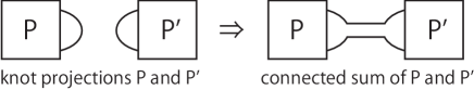
The connected sum of two knot projections and are defined by Fig. 7.
Theorem 4.
Let be an arbitrary knot projection. has the following properties.
-
(1)
is an odd integer.
-
(2)
where is a connected sum of and .
-
(3)
For a knot projection , we give an arbitrary orientation. If contains an element of the following list (Fig. 8) as a sub-diagram, .

Figure 8. List of -gons.
Proof.
-
(1)
By the definition, is . It is well known that an arbitrary knot projection and the simple circle can be related by a finite sequence of the first, second, and third flat Reidemeister moves, where the first and second flat Reidemeister moves are defined by Fig. 1 and the third flat Reidemeister move is defined by Fig. 9.

Figure 9. The third flat Reidemeister move. We have already shown that is invariant under RI and strong RII. Thus, it is sufficient to show that (mod ) under weak RII and the third flat Reidemeister move.
First, let us consider weak RII by looking at Fig. 10. For a knot projection with an orientation (the upper-left of Fig. 10), we have appearing as in the left figure of the second row. We consider the possibilities of the connections of arcs of finitely many simple circles which we focus on. We can draw them as locally two types of , as in the upper right of the first and second rows in Fig. 10. These two figures imply that is either or if and is related by a single weak RII.

Figure 10. The symbol in the figure (upper part) stands for weak RII. In the lower part of the figure, the symbol (resp. ) represents the weak (resp. strong) RIII. Next, we consider the third flat Reidemeister move. The third flat Reidemeister move can be split into the two kinds of moves by the way of connection of three branches as in Fig. 9 (see Fig. 11).

Figure 11. The strong (upper) and weak (lower) RIII. The upper (resp. lower) local move of Fig. 11 is called the strong (resp. weak) RIII.
These two local moves can be detected easily by giving an orientation to a knot projection. In fact, one appears in the left of the third line and the other appears in the fourth line of Fig. 10 if any orientations of knot projections are given.
We apply non-Seifert resolutions to the two types of the third flat Reidemeister move (the left column in the third and fourth lines of Fig. 10). Therefore, it is sufficient to consider to the two cases of connections of three arcs that are parts of simple circles (the bottom line of Fig. 10). The two figures in the bottom line of Fig. 10 shows that is either or if a knot projection is related to the other knot projection by a single third flat Reidemeister move. This completes the proof of (1).
-
(2)
For two knot projections and , we give them any orientations, and denote by and these oriented knot projections. The knot projection with the opposite orientation is denoted by . Now we consider a connected sum of and . We can preserve the orientation of under this connected sum by choosing either or . Note that the . Apply non-Seifert resolution at all double points . The way of smoothing them is the same as those for and since we consider either or .
-
(3)
If there exists at least one part as one of the list, we have at least two circles in . By (1), we have .
∎
Remark 2.
Let be a knot projection and set , where and are Arnold invariants of immersed plane curves when we assign to one arbitrary chosen region. It is easy to see that does not depend on the choice of and is an invariant of knot projections [9, Page 997, Corollary 2]. Moreover, it is easy to note that is invariant under strong (1, 2) homotopy.
We can also demonstrate that is independent of . For instance, let (resp. ) be the simple circle (resp. the trefoil projection) and let (resp. ) be the (resp. ) projection as shown in Fig. 20. On one hand, , , and . On the other hand, , , and . As previously demonstrated, circle arrangement is strictly stronger than circle number, and as shown in Fig. 20, , , , and are all mutually different.
5. Proof of Theorem 2
In this section, we prove Theorem 2. To avoid confusion, recall that the symbol (resp. ) represents strong (1, 2) homotopy (resp. weak (1, 2) homotopy) (see the definition of and in the statement of Theorem 1).
Proof.
The assumption is that there exists a knot projection such that is equivalent to the simple circle up to weak (1, 2) homotopy (i.e. ) and is also equivalent to up to strong (1, 2) homotopy (i.e. ). The condition that implies that . On the other hand, implies that there exists a finite sequence () of and from to by Lemma 1.
Now, we assume that the sequence () contains at least one (). Therefore, there exists a knot projection with at least one incoherent -gon such that . Then, . By Theorem 4 (3), is a contradiction. Thus, the assumption () is false and then the sequence () contains only . Then .
Conversely, assume that . Then, in particular, satisfies both and . This completes the proof of Theorem 2. ∎
6. Properties of circle arrangements
We call a prime knot projection if is non-trivial and cannot be a connected sum of non-trivial knot projections.
Theorem 5.
For any circle arrangement , there exists a knot projection such that . In particular, for any positive integer , there exists a knot projection such that .
Moreover, we can choose a prime knot projection as .
Lemma 3.
A circle arrangement can be locally changed as in Fig. 12 from to by considering a connected sum if is the trefoil projection or projection where the trefoil projection and projection look as in Fig. 12.

Proof.
It is easy to see this proof by the definition of the circle arrangement. ∎
Lemma 4.
Let be a knot projection and assume . There exists a -disk on the -sphere such that contains exactly two circles that are separated or nested in as illustrated in Fig. 13.

Proof.
Lemma 5.
There exists a finite sequence generated by and to obtain a prime knot projection from any non-prime knot projection.
Proof.

If a knot projection is a simple curve, it is easy to see that projection (cf. Fig. 20) is obtained by and . In the following, we assume that a knot projection is a non-trivial knot projection. We consider a prime decomposition as Fig. 14. If a knot projection has a non-trivial sub-curve such that the sub-curve has exactly two end points and if we can find a simple arc closing the two endpoints of the curve that produces a prime knot projection and where the closing does not create double points, then the non-trivial sub-curve is called a prime part of . Let us encircle the prime part at one of the most inner regions by one circle, called a red circle, where we arbitrarily select an innermost prime part. If we replace the prime part with a simple arc, we precede to the next stage and repeat; we encircle the prime part of one of the innermost regions by a red circle that must not intersect the other red circles. We continue to draw red circles not intersecting the other red circles. Finally, we draw a circle whose part is contained by the outermost region and select a next-innermost prime part and repeat the above process. For each step, if the outermost red circle is already given by the former process, we omit drawing it (e.g., Fig. 14). Since the number of double points in a knot projection is finite, every encircling must eventually stop. As a result, we can choose a decomposition where each red circle contains a prime part where we replace prime parts with simple arcs if the other red circles are contained in .

Let us look at Fig. 15. Every red circle can be drawn as in Fig. 15. Call the two arcs of Fig. 15 marked arcs. Every arc of the sub-diagram within the red circle of Fig. 15 is called a prime part’s arc. Choose two non-marked arcs and in the same region where one is picked from a prime part’s arc and the other is picked from a distinct neighboring prime part’s arc . Apply the operation shown in Fig. 16 to arcs and . This operation is one or a pair of and ; if two arcs and cannot make a coherent -gon directly, we make the allowable situation by applying one (see Fig. 16).

As a result, the relation of the two neighboring prime parts is not a connected sum and so we should delete the red circle between the two prime parts. We apply this operation to every red circle, and so we can eventually resolve all the connected summations to obtain a prime knot projection. Thus, the proof is completed. ∎
Next, we prove Theorem 5.
Proof.
If , by Theorem (1). We have (the symbol presents a knot projection, see Fig. 20). Thus, we can assume that in the following. Let (resp. ) be the left (resp. right) figure of Fig. 13. By Lemma 4, we can find at least one copy of either or within any arbitrary circle arrangement. For such an arbitrary circle arrangement , obtain by deleting this part, denoted by or . In , we can find at least one copy of or which we denoted by . Repeating the deletions, we eventually have exactly one circle and a sequence for some positive integer .
Next, we will construct any circle arrangement from one circle . For one circle , we put in the two regions given by on . Using Lemma 3, if (resp. ), we consider the connected sum of the trefoil (resp. ) projection and as in Fig. 12. Next, for , we consider an appropriate connected sum by specifying and . By applying connected sums step by step as above, we finally obtain a knot projection such that and consists of finitely many trefoil and projections.
Next we consider the goal of obtaining a prime knot projection such that . To obtain such a knot projection, every time we consider a connected sum in the above step , we apply an operation or a pair as Fig. 16 (e.g., Fig. 17).

∎
7. Table of circle numbers and circle arrangements
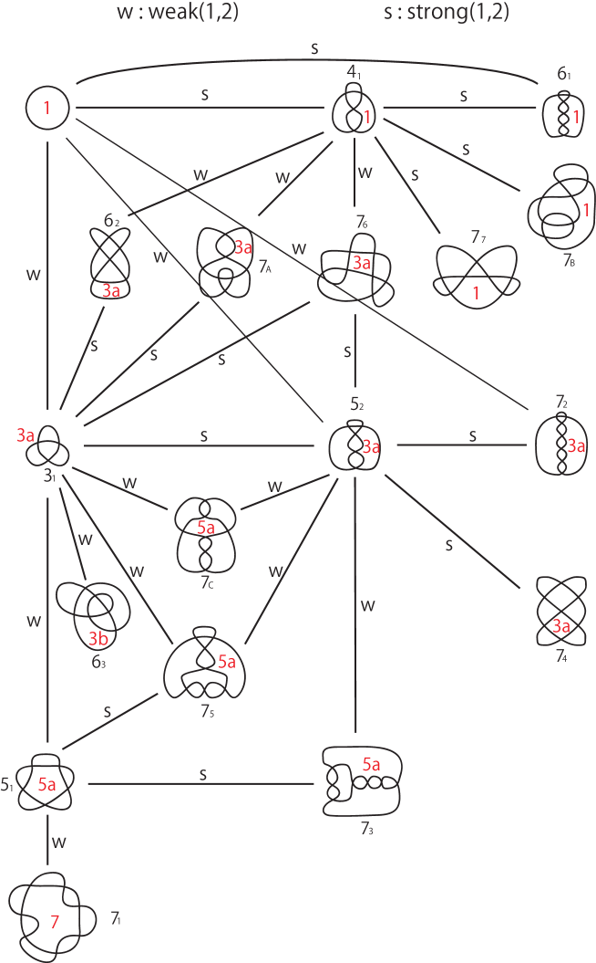
Finally, we include a table of circle invariants on prime knot projections without -gons up to seven double points (Fig. 20). The symbols for circle arrangements appearing in Fig. 20 are defined by Fig. 19. Note that the following two points. The first point explains the meaning of the symbols , , and . Traditionally, denotes the projection image of the knot in Rolfsen table. To tabulate prime knot projections without -gons up to seven double points, all knot projections are obtained from by flypes of knot projections defined by Fig. 18 (cf. Tait Conjecture).

Thus, exactly three knot projections should be added, i.e., (from ), (from ), and (from ). The second point is that we obtain the definitions of lines with and in Fig. 20. Two knot projections are connected by a line with (resp. ) if a finite sequence generated by moves of type and a single (resp. ) that connects the two knot projections is found.

Acknowledgements
The authors would like to thank Professor Kouki Taniyama for his fruitful comments. The authors would also like to thank the referee for his/her comments on an earlier version of this paper. The part of this work of N. Ito was supported by a Waseda University Grant for Special Research Projects (Project number: 2014K-6292) and the JSPS Japanese-German Graduate Externship. N. Ito is a project researcher of Grant-in-Aid for Scientific Research (S) 24224002 (April 2016–).
References
- [1] V. I. Arnold, Topological invariants of plane curves and caustics, University Lecture Series, 5. American mathematical Society, Providence, RI, 1994.
- [2] R. Fenn, Techniques of geometric topology, London Mathematical Society Lecture Note Series, 57. Cambridge University Press, Cambridge, 1983.
- [3] R. Fenn and P. Taylor, Introducing doodles, Topology of low-dimensional manifolds (Proc. Second Sussex Conf., Chelwood Gate, 1977), pp.37–43.
- [4] N. Ito and A. Shimizu, The half-twisted splice on reduced knot projections, J. knot Theory Ramifications 21 (2012), 1250112, 10pp.
- [5] N. Ito and Y. Takimura, (1, 2) and weak (1, 3) homotopies on knot projections, J. Knot Theory Ramifications 22 (2013), 1350085, 14pp.
- [6] N. Ito, Y. Takimura, and K. Taniyama, Strong and weak (1, 3) homotopies on knot projections, Osaka J. Math. 52 (2015), 617–646.
- [7] M. Khovanov, Doodle groups, Trans. Amer. Math. Soc. 349 (1997), 2297–2315.
- [8] A. Shumakovitch, Explicit formulas for the strangeness of plane curves, (Russian) Algebra i Analiz 7 (1995), 165–199; translation in St. Petersburg Math. J. 7 (1996), 445–472.
- [9] M. Polyak, Invariants of curves and fronts via Gauss diagrams, Topology 37 (1998), 989–1009.
- [10] O. Viro, Generic immersions of the circle to surfaces and the complex topology of real algebraic curves, Topology of real algebraic varieties and related topics, 231–252, Amer. Math. Soc. Transl. Ser. 2, 173, Amer. Math. Soc., Providence, RI, 1996.