Streamer discharge simulations in humid air: uncertainty in input data and sensitivity analysis
Abstract
We study how the choice of input data affects simulations of positive streamers in humid air, focusing on H2O cross sections, photoionization models, and chemistry sets. Simulations are performed in air with a mole fraction of 0%, 3% or 10% H2O using an axisymmetric fluid model. Five H2O cross section sets are considered, which lead to significant differences in the resulting electron attachment coefficient. As a result, the streamer velocity can vary by up to about 50% with 10% H2O. We compare results with three photoionization models: the Naidis model for humid air, the Aints model for humid air, and the standard Zheleznyak model for dry air. With the Naidis and in particular the Aints model, there is a significant reduction in photoionization with higher humidities. This results in higher streamer velocities and maximal electric fields, and it can also cause streamer branching in our axisymmetric simulations. Three humid air chemistry sets are considered. Differences between these sets, particularly in the formation of water clusters around positive ions, cause the streamer velocity to vary by up to about 50% with 10% H2O. A sensitivity analysis is performed to identify the most important chemical reactions in these chemistries.
1 Introduction
Streamers are fast-propagating and filamentary ionization fronts featuring an enhanced electric field at their tips [1]. This field enhancement enables streamers to propagate in sub-breakdown background fields and therefore to serve as precursors to more energetic phenomena such as sparks and lightning leaders [2, 3]. Streamers are also fundamental blocks of some transient luminous events (TLEs) that occur in the upper atmosphere, including sprites and blue jets [4]. Although streamers are low-temperature plasmas, the strong electric field at the streamer head can accelerate electrons to really high energies and thus, can trigger high-temperature chemical reactions at nearly room temperature [5]. This property has been harnessed for numerous applications such as plasma medicine [6], agriculture [7], industrial surface treatments [8], air cleaning [9], plasma-assisted combustion [10], and non-thermal plasma actuators [11].
The gas composition affects streamer properties such as velocity, radius, breakdown field, and branching characteristics, as well as the plasma species produced by streamers [12, 13, 14, 15]. Frequently, water vapor is a component of gas mixtures. When studying streamer-like discharges in atmospheric air for plasma medicine and agriculture applications, in supersaturated air inside a thundercloud, or in high-voltage power transmission systems under complex environmental conditions, humidity is an important factor that cannot be neglected. Below, we briefly discuss some relevant experimental and computational studies that account for air humidity.
In the late 1970s, the pioneering experimental works by Griffiths and Phelps [16, 17], Les Renardiers group [18, 19] and Gallimberti [2], showed that water vapor hampered streamer propagation in long air gaps. Therefore, the stability field (i.e., the minimal average electric field required for bridging an air gap) increased with increasing water vapor content [20, 21, 22]. For example, in [20] such a stability field was measured at 5.24 kV/cm at an absolute humidity of 11 g/m3, and it increased by about 1.3% for every 1 g/m3 increase in the humidity. Furthermore, the field required for a streamer to cause breakdown also increased with increasing air humidity at a rate of about 0.56% per g/m3 [22]. Zhao et al experimentally investigated the effect of humidity on the evolution of streamer dynamics and discharge instabilities under repetitive pulses [23, 24], finding increased branching in both primary and secondary streamers in humid air. In addition, air humidity leads to the formation of OH radicals in streamer discharges. It was observed that an increase in humidity resulted in increased OH density but a decrease in O3 production due to lower atomic oxygen levels [25, 26, 27]. Increased humidity was also found to enhance fast gas heating for streamer discharges in humid air [28, 29, 30].
There are also numerous computational studies regarding how humidity affects streamer propagation in atmospheric air, using 1.5D (assuming a constant radius of the streamer channel) [31, 21], as well as 2D [32, 33, 34, 35] and 3D ‘discharge tree’ [36] models. These simulations showed that the influence of humidity became noticeable in long streamer discharges. As air humidity increased, the streamer propagated more slowly with a smaller radius, and the background field required for sustaining streamer propagation was also higher, in agreement with previous experimental findings [16, 17, 18, 19, 2, 20, 21, 22]. This humidity effect on streamer properties was primarily attributed to reduced conductivity in the streamer channel, due to dissociative recombination of electrons with positive cluster ions and enhanced three-body electron attachment to O2 molecules [33, 34]. The above effects can be weakened by increasing the gas temperature. According to [32], higher gas temperatures reduced the rates of electron recombination and three-body attachment reactions, which in turn increased the conductivity of the streamer channel. Furthermore, air humidity had a significant impact on the electron swarm parameters needed for fluid streamer simulations, thereby influencing streamer properties, as discussed in [37].
One of the main challenges in modeling streamers (or other discharges) in humid air is selecting appropriate input data. For example, different electron-neutral cross sections for H2O were used in [38, 32, 33, 34, 39], as well as different cross sections for N2 and O2. In [40], a simplified reaction set was used for streamer simulations in humid air. To obtain more complete and reliable kinetic data, a recommended database was constructed for humid air plasma chemistry in [41, 42]. Based on these early humid air chemistries, various sets of chemical reactions were further developed in subsequent simulation studies [38, 32, 33, 34, 39] under different discharge conditions. Of particular importance are the cross sections for three-body electron attachment to H2O, as well as the reactions related to the production of cluster ions and the corresponding electron-ion recombination rates [43]. Furthermore, most of the above-mentioned simulations did not account for the effect of H2O on photoionization, despite its significance.
In this paper, we investigate how the choice of input data affects streamer properties such as the streamer velocity, optical diameter, and maximal electric field. We consider different H2O cross section sets, different photoionization models and different sets of chemical reactions to study their effects on single positive streamers in humid air.
2 Simulation model
We perform axisymmetric simulations of positive streamers with the Afivo-streamer code [44], using a drift-diffusion fluid model with the local field approximation. The model is briefly described below, for further details see e.g. [44, 45].
The simulations are performed in gas mixtures containing N2 and O2 at a 4:1 ratio together with H2O. We consider three humidities, with a mole fraction of 0%, 3% and 10% H2O, as listed in table 1. Note that we slightly vary the gas temperature and pressure to obtain humid air with 10% H2O but keep the gas number density the same.
| Case | H2O | N2 | O2 | P (bar) | T (K) |
|---|---|---|---|---|---|
| 1 | 0.0% | 80.0% | 20.0% | 1.0 | 300 |
| 2 | 3.0% | 77.6% | 19.4% | 1.0 | 300 |
| 3 | 10.0% | 72.0% | 18.0% | 1.067 | 320 |
2.1 Equations
In our model, the electron density evolves in time as
| (1) |
where and are the drift and diffusive fluxes of electrons, the electron mobility, the diffusion coefficient, and the electric field. Furthermore, is an electron source term due to reactions (e.g., ionization or attachment) described in section 2.5, and is the photo-ionization source term described in section 2.4. Electron transport coefficients are assumed to depend on the local electric field, and they were computed with BOLSIG [46] using the cross sections described in section 2.3.
We consider time scales up to about and found that including ion mobilities made no significant difference in our results. The motion of ions is therefore neglected, so that ions and neutral densities (numbered by ) evolve in time as
| (2) |
where is a source/sink term due to reactions.
2.2 Computational domain and initial condition
We use a 2D axisymmetric computational domain measuring in the and directions, which contains a plate-plate geometry with a needle electrode (8 mm in length and 0.8 mm in diameter), as illustrated in figure 1. The bottom plate is grounded, whereas a constant high voltage is applied on the upper plate and the needle electrode. The axial electric field away from the needle electrode relaxes to the average electric field between the two plate electrodes, which is here defined as the background electric field :
| (4) |
where mm is the distance between two plate electrodes.

For the electrostatic potential, a homogeneous Neumann boundary condition is used on the outer radial boundary. For all species densities, homogeneous Neumann boundary conditions are used on all domain boundaries, including the needle electrode. Secondary electron emission from electrodes due to ions and photons is not included.
As an initial condition, homogeneous background ionization with a density of for both electrons and N ions is included. All other ion densities are initially zero. This background ionization provides the first electrons for streamer inception near the electrode tip, where there is significant electric field enhancement.
For computational efficiency the simulations are performed using adaptive mesh refinement (AMR). We use the same refinement criteria as in previous works (see e.g.[44]), namely to refine when and to de-refine when , where is the field-dependent ionization coefficient and is the grid spacing. The minimum grid spacing in the simulations was . Around the needle electrode, we enforce .
2.3 Electron-neutral cross sections for N2, O2 and H2O
Electron-neutral collisions are the dominant process in streamer discharges, and energy-dependent probabilities of such collisions are described by cross sections. In a fluid model these cross sections are used indirectly through a Boltzmann solver to obtain electron transport coefficients (such as the mobility) and rates for electron-neutral reactions. BOLSIG [46] with the temporal growth model was used to obtain such data.
For most atoms and molecules, there is still quite some uncertainty in the electron-neutral cross sections. For example, in [49] streamer simulations were compared using different cross section sets for dry air (80% N2, 20% O2), and it was found that the streamer velocity could vary by about 10% when compared at the same position. Although the gas mixtures considered here consist mostly of N2 and O2, we here want to focus on the uncertainty in cross sections for H2O. All simulations are therefore performed using Phelps’ cross sections for N2 and O2 [50, 51, 52], whereas for H2O we consider the cross section sets described below.
We emphasize that the choice of H2O cross section sets included in our comparison was rather arbitrary, and that we probably could have included other data as well (from e.g., [53, 54, 55]). However, our goal here is simply to illustrate how much variation there will be in streamer simulations using different H2O cross section sets. For a more extensive discussion of H2O cross sections and their accuracy, we refer to [56, 53, 57, 55].
2.3.1 Kawaguchi H2O cross sections
The cross section set of Kawaguchi et al [57] was compiled based on several previous sources (too many to list here), and it contains about 40 cross sections for rotational, vibrational and electronic excitations, ionization and electron attachment. With Monte Carlo swarm simulations, the authors demonstrate that their set reproduces experimental swarm measurements better than those of [54, 58, 53]. What furthermore makes this set attractive to use is that they also provide a set with an isotropic scattering model. The tabulated cross sections were obtained by contacting the authors directly, but the authors plan to also make them available at lxcat.net.
2.3.2 Morgan and Phelps H2O cross sections
Through lxcat.net [59], we obtained the Morgan [60] and Phelps [61] cross section sets for H2O. For both of these, there is the following warning: “This cross section set should not be used in Boltzmann calculations because it does not include explicitly rotational cross sections (very important in H2O). Morgan used an analytical form for these cross sections.” Although values for the “continuous approximation to rotation” (CAR) are given by Morgan, we were not able to reconstruct a reasonable looking rotational cross section using the formulas in [62], in particular due to uncertainty in the units used. For comparison we nevertheless include these sets without rotational cross sections.
We remark that in the recently published paper by Budde et al [55] the lack of rotational cross sections for H2O is extensively addressed. The authors provide a complete set containing 147 rotational cross sections, out of a total of 163 cross sections. The set is tested against swarm measurements using two two-term Boltzmann solvers, and the authors obtain good agreement. At the time of writing, this set was not yet available on lxcat.net, so we did not include it in our comparison.
2.3.3 Triniti H2O cross sections
We also obtained the Triniti set [63] through lxcat.net, which was obtained from the EEDF Boltzmann solver [64]. The cross section file includes a reference to Yousfi et al 1987, which we could not find, but this suggests that these cross sections could be related to the ones published later in [54].
2.3.4 Itikawa H2O cross sections
The review paper by Itikawa et al [58, 65] provides an overview of available cross sections for H2O together with recommendations, which are available at lxcat.net. An update of these cross sections was recently given in [66]. We want to briefly mention two caveats when using this data. First, due to the strong dipole moment of H2O, elastic scattering is highly anisotropic and sharply peaked in the forward direction. Although a total momentum transfer cross section is provided, the cross sections cannot directly be used in a Boltzmann solver that assumes isotropic scattering, since the set also includes rotational excitations that have to be described anisotropically. A second caveat is that some of the cross sections are only given up to a certain energy (which can be as low as ) at which they are still nonzero. If such cross sections are used in a Boltzmann solver, it depends on the particular implementation how they will be extrapolated above this energy range.
Although the data of [58] should only be used with an appropriate anisotropic scattering model, we include it here in an improper way, just for comparison with the Morgan and Phelps data. For this comparison, we have removed all rotational cross sections from the Itikawa set.
2.3.5 Comparison of electron transport coefficients
We have used the cross section sets described above to compute electron transport coefficients using BOLSIG- [46]. Figure 2 shows results for a hypothetical scenario with pure H2O gas at and . There is considerable variation between the five sets for all transport parameters, which is not that surprising since the Morgan, Phelps and Itikawa data are used in an inappropriate way, as discussed above. The Morgan, Phelps and Itikawa data show higher ionization coefficients compared to the other two sets. The Morgan data leads to a substantially higher diffusion coefficient and a rather flat mobility. The Itikawa data yields a higher attachment coefficient and a higher peak mobility at a lower electric field. Furthermore, the Kawaguchi and Triniti sets agree quite well in terms of the ionization coefficient. For the attachment coefficient, we find good agreement between Kawaguchi and Morgan and between Triniti and Phelps.

Figure 3 shows results for air with 3% and 10% H2O at and . As expected, for both air humidities the differences in the transport coefficients between the five sets are now much smaller, due to the smaller contribution of the H2O cross sections. The attachment coefficient now has a peak at low electric fields due to three-body attachment reactions:
| (5) |
| (6) |
where for this comparison reaction (6) was assumed to have a rate coefficient six times that of reaction (5). For air with 10% H2O, the maximum difference in the resulting attachment coefficients is about 20%, whereas the variation in the ionization coefficient is below 5%. For the case of 3% H2O, the differences in the transport coefficients are even smaller and difficult to see, with the maximum variation in the attachment coefficient being about 8%. Note that regardless of the specific H2O cross section set used, a decrease in the mole fraction of H2O from 10% to 3% results in a lower attachment coefficient, but hardly affects other transport parameters.

2.4 Photoionization
Photoionization in humid air resembles that in dry air: excited N2 molecules can emit photons with enough energy to non-locally ionize O2 molecules, see e.g. [67]. We consider two approaches for modeling photoionization in humid air, which are described below. For comparison, we also briefly describe the dry air case.
2.4.1 Dry air - Zheleznyak’s model
In dry air, the production (per unit time and volume) and absorption (per unit distance) of these photons are here approximated using Zheleznyak’s model [68]. In this model, is proportional to the electron impact ionization source term :
| (7) |
where is the quenching pressure, the gas pressure, and is a proportionality factor, which is here set to as in e.g. [69, 70]. Furthermore, the absorption function is given by
| (8) |
where , and is the partial pressure of O2. We remark that what actually matters is the number density of O2 molecules, but we here follow the usual assumption of the gas being at room temperature.
2.4.2 Humid air - Naidis model
Naidis [71] proposed a simple modification of Zheleznyak’s model, in which water molecules lead to extra absorption:
| (9) |
where and is the partial pressure of H2O. Note that with this extra term, the integral (from 0 to ) over the absorption function is less than unity, because the photons absorbed by H2O do not contribute to photoionization.
2.4.3 Humid air - Aints model
Aints et al [72] performed measurements on photoionization in humid air that were not consistent with equation (9) for small values of . They therefore proposed a different absorption function which we here write as
| (10) |
where and , with and . Note that this absorption function has an integral of unity. The authors instead introduced additional quenching by H2O in equation (7):
| (11) |
which was fitted against their data to obtain . We use the above expressions, but remark that the value of appears unrealistic, since gas molecules do not collide (or interact) frequently enough to warrant such a low quenching pressure [73].
2.4.4 Numerical implementation
We implement photoionization in our fluid model with the Helmholtz approach, as described in [74, 75]. We used an expansion with three Helmholtz terms of the form
| (12) |
where corresponds to equation (7) or (11), and the coefficients and are given in table 2. See e.g. Appendix A of [45] for more details about this type of expansion.
. Case Model (mm-1) (mm-2) 0% H2O Zheleznyak 0.830 2.19 13.4 0.0447 1.15 110 3% H2O Naidis 1.51 3.88 32.5 0.0863 3.89 757 3% H2O Aints 1.21 3.59 32.6 0.0963 4.37 875 10% H2O Naidis 2.83 5.19 33.0 0.0858 3.83 697 10% H2O Aints 1.86 4.24 33.3 0.114 5.18 1045
2.5 Chemical reactions
In addition to electron-neutral cross sections, chemical reactions are another important input data for streamer fluid simulations. For many reactions, there are significant uncertainties in both the reaction form and the reaction rate coefficient, see e.g. [76, 77]. Furthermore, previous authors have used different sets of chemical reactions for humid air, and it is often unclear which set is the most suitable and which reactions are most significant.
In this work, we use the three chemistry sets that are described below. We have made small modifications to these sets so that they are compatible with the electron-neutral cross sections that we use. We have also included reactions to obtain the emitted light from the second positive system (), which is responsible for most of the optical emission in air at atmospheric pressure [78]. Furthermore, we have made corrections to reaction rates when necessary. All these changes are documented in B.
We remark that the choice of chemistry sets was also arbitrary, with the sets obtained from recent papers for streamer simulations in dry/humid air. There are other datasets, e.g., from [39, 41, 42]. Our purpose here is simply to demonstrate how sensitive streamer simulations are to the use of different datasets.
2.5.1 Humid air - Malagón chemistry set
This chemistry set for streamer simulations in humid air is based on the reactions from Malagón-Romero et al [33], and it is listed in table 4. This set contains 97 chemical reactions, which can be divided into eight different processes: electron impact ionization, electron attachment, electron detachment, negative ion conversion, positive ion conversion, electron-ion recombination, ion-ion recombination, and light emission. For most reactions of ion-ion recombination, reaction products were not given.
2.5.2 Humid air - Starikovskiy chemistry set
This chemistry set for humid air is based on Starikovskiy et al [34], as given in table 5. The set contains only 72 chemical reactions and six processes. Compared to the Malagón chemistry set described above, it does not include electron detachment and negative ion conversion processes. Additionally, it includes a single negative ion O as compared to Malagón’s which includes seven negative ions. Finally, the rate coefficient for three-body attachment with H2O (reaction R10) is seven times that of three-body attachment with O2 (reaction R9) rather than six times in the Malagón chemistry set. Note that for dissociative recombination of electrons with ions, the range is used in this set. However, in the paper they cite for this reaction [79] only ranged from 1 to 4.
2.5.3 Humid air - Komuro chemistry set
This chemistry set for humid air is based on Komuro et al [38, 32], as listed in table 6. Compared to the previous two sets, this set contains many more chemical reactions (191 reactions in total) and eleven types of processes, resulting in some differences. First, it contains several excited species, summarized in table 7. Second, it contains electron dissociation reactions (R13–R16), which effectively produce neutral atoms that are needed for neutral species conversion. Third, it contains neutral species conversion as the reactions were collected for studying the behavior of OH radicals in streamer discharges in [38]. Furthermore, as stated in [32], this chemistry set was constructed to investigate the effect of gas temperature rather than humidity. Therefore, some (important) reactions related to water cluster ions, such as the recombination reactions of electrons with ions, were not taken into account.
2.5.4 Dry air - Guo chemistry set
This chemistry set from Guo and Teunissen [80] was constructed for streamer simulations in dry air. It contains 263 chemical reactions and twelve processes, which were primarily based on the reactions from [81, 82]. This set is not listed in B as it is completely the same as the one in [80]. For further comparison, we obtained three other chemistry sets for dry air by removing the reactions related to H2O from the above three humid air chemistry sets.
2.6 Sensitivity tests
We use so-called sensitivity tests [83] to better understand which chemical reactions are important. These tests are performed by multiplying individual reaction rate coefficients with a factor for , using the following values: . With reactions, the total number of additional simulations is thus . We then pick a “quantity of interest”, here called , that we compare at some particular time to the case with unmodified rate coeffients . For reaction there are then results for , from which we compute normalized derivatives as
| (13) |
where . Finally, we determine the mean of the normalized derivatives
| (14) |
and the sample standard deviation of the
| (15) |
Note that there are more sophisticated ways to do sensitivity tests in which multiple coefficients are varied at the same time, see e.g. [77, 84, 85]. However, our purpose here is simply to understand which reactions are important, and not to quantify the uncertainty in results due to uncertainties in the rate coefficients.
3 Simulation results
Below we will study how the H2O cross sections, the photoionization model and the chemistry set affect simulations of positive streamers in humid air. We will compare the following streamer properties:
-
•
The maximal electric field at the streamer head. The location of this maximum is defined as the streamer head position.
-
•
The velocity , obtained as the time derivative of the streamer head position.
-
•
The optical diameter , defined as the full width at half maximum (FWHM) of the time-integrated light emission after a forward Abel transform, see e.g. [49]. This simulated optical diameter can be used for comparison with experimental data.
3.1 Effect of H2O cross sections
As described in section 2.3, five cross section sets for H2O were considered, namely Kawaguchi, Triniti, Morgan, Phelps, and Itikawa. We remind the reader that rotational cross sections were not included in the Morgan and Phelps data, and that we left them out for the Itikawa data. In this section, we investigate the effect of these H2O cross sections on positive streamers in humid air with 3% and 10% H2O. The simulations were performed in a background field of 10 kV/cm, using the ‘dry air’ Zheleznyak photoionization model and the chemistry set of Malagón.
We first illustrate a typical time evolution in these simulations on the left of figure 4, which shows the electric field and electron density profiles for the streamer in air with 3% H2O using the Kawaguchi H2O cross sections. The streamer starts from the needle electrode and accelerates downwards, with the velocity and the optical diameter increasing approximately linearly with time, from about m/s to m/s and from about 1.2 mm to 3.7 mm, respectively. However, the maximal electric field at the streamer head remains approximately constant at about 110 kV/cm.
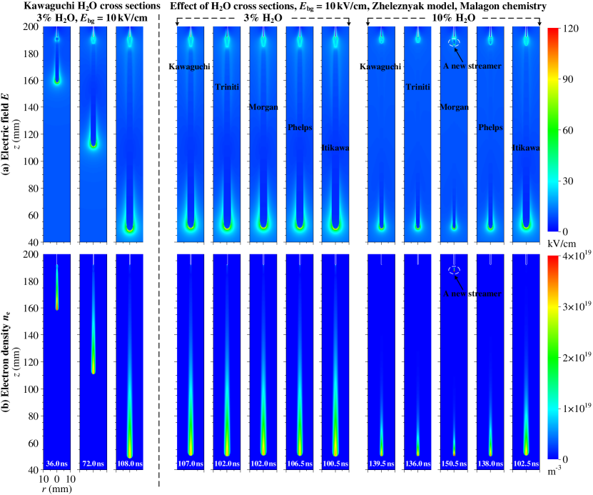
Simulations with different H2O cross sections are compared on the right of figure 4, which shows the electric field and electron density profiles for air with 3% and 10% H2O, at the moment the streamers reach mm. In addition, the maximal electric field, streamer velocity, and optical diameter are shown versus the streamer head position in figure 5.
In air with 3% H2O, all five different cross sections do not lead to obvious differences in streamer properties, with variations below 10% when compared at the same streamer length. This is not that surprising, as differences in the electron transport coefficients are also small with 3% H2O, as mentioned in section 2.3.5. Differences become larger with 10% H2O in air, and then three groups can be distinguished: ① the Kawaguchi, Triniti and Phelps cases, which show good agreement; ② the Morgan case; and ③ the Itikawa case. Compared to the cases with 3% H2O, streamers in group ① become about 40% slower and thinner, due to a much faster decay of conductivity in the streamer channel. The Morgan case shows even slower propagation at about m/s and a smaller diameter of about 1.4 mm, which is attributed to a higher attachment coefficient, as demonstrated in figure 3. An interesting phenomenon occurs in the Morgan case where a new positive streamer is generated from the needle electrode behind the previous one. This phenomenon, recently observed in strongly attaching gases in [15] as well, will be further illustrated in A. In contrast, the Itikawa case propagates much faster with a larger diameter, similar to those with 3% H2O, but with a slightly lower . Although the attachment coefficient in the Itikawa data is nearly identical to that in the Morgan data, the ionization coefficient is about 5% higher. This suggests that ionization reactions play a more significant role than attachment, as discussed in A.

In the rest of the paper, we will use the Kawaguchi H2O cross sections, as they can reproduce experimental swarm measurements and because they can be used with an isotropic scattering model, see section 2.3.1.
3.2 Effect of the photoionization model
We now compare different photoionization models to understand how important changes in photoionization due to humidity are. Three approaches are considered: the Naidis and Aints models for humid air discussed in section 2.4, and for comparison also the standard Zheleznyak model for dry air described in section 2.4.1. We performed simulations with these models using the Malagón chemistry and the Kawaguchi H2O cross sections, in a background field of 10 kV/cm. Figure 6 shows the electric field and electron density profiles when the streamers have reached , and corresponding axial profiles are shown in figure 7. Furthermore, figure 8 shows streamer properties as a function of the streamer head position .


There is a clear effect of photoionization on and other streamer properties. If the standard Zheleznyak model is used, is almost the same for air with 0%, 3% and 10% H2O. However, other streamer properties such as velocity and diameter vary significantly, with a higher humidity leading to a reduced velocity and diameter. With the Naidis and Aints models there is less photoionization, which leads to an increase in of up to about 15%. Due to the higher field at the streamer tip, the electron density in the streamer channel is also higher. Furthermore, the streamer velocity is substantially higher, for example about 30% higher with the Naidis model and 10% H2O than with the Zheleznyak model. The effect on the streamer diameter is smaller, with differences of up to about 15% between the Naidis and Zheleznyak cases for 10% H2O.
In addition, the reduction in photoionization with the Naidis and Aints models can cause the axisymmetric streamers to become unstable and eventually branch, which happens with the Aints model and 10% H2O. Since we cannot simulate branching with the axisymmetric fluid model used here, this case was not included in the figures. Performing realistic simulations of the branching dynamics of streamers in humid air would require fully 3D simulations, as well as a stochastic treatment of photoionization [70, 86, 69], which we leave for future work.
That a reduction in photoionization can lead to faster streamers was also found in previous work [49]. Perhaps this is most easily understood from the scenario in which there is a very large amount of photoionization. In such cases, the streamer will have less field enhancement, and thus become less conductive, which means that it will propagate more slowly.
3.3 Effect of the chemistry set
In this section, we study the effect of chemical reactions on positive streamers in humid air. We used the chemistry sets described in section 2.5 with varying humidity levels to perform a total of ten streamer simulations, for which the conditions are summarized in table 3. Figure 9 shows the electric field and electron density profiles when the streamers have reached mm, and figure 10 shows streamer properties as a function of the streamer head position .
| Chemistry | Photoionization model | H2O (%) |
|---|---|---|
| Guo | Zhelezhnyak | 0 |
| Komuro | Zhelezhnyak, Naidis | 0, 3, 10 |
| Malagón | Zhelezhnyak, Naidis | 0, 3, 10 |
| Starikovskiy | Zhelezhnyak, Naidis | 0, 3, 10 |


The chemistry set also has an important effect on streamer properties. We first look at the maximal electric field at the streamer head. For each humidity considered here, there are almost no differences in with different chemistry sets. However, an increase in air humidity leads to a higher .
We then focus on the streamer velocity and diameter. As a first test, we compare results in dry air (0% H2O) with the four considered chemistry sets, since these chemistries also differ in the included reactions for oxygen and nitrogen species. Streamers with the Komuro and Malagón chemistries agree very well in this case, whereas the Starikovskiy and Guo chemistries lead to slower streamers. At mm, the Starikovskiy case is about 8% slower, whereas the Guo case is about 12% slower. In streamer diameter these differences are about 10% and 14%, respectively.
Next, we compare results in humid air with 3% and 10% H2O using the Komuro, Malagón and Starikovskiy chemistries. The differences in streamer velocity then become larger, with the Komuro case leading to the fastest streamers and the Starikovskiy case leading to the slowest ones. With 3% H2O, the Malagón case is about 15% slower than the Komuro case at mm, and the Starikovskiy case is about 35% slower. With 10% H2O, these differences are about 15% and 50%, respectively. The differences in streamer diameter are approximately the same as those in the velocity, with the slower streamer having a smaller diameter. Note that the Starikovskiy case with 10% H2O is approximately a steady positive streamer, whose properties do not vary in time, as discussed in [14].
Regardless of the particular chemistry, an increase in the percentage of H2O leads to slower streamers with a smaller diameter, as was also found in previous work [33, 34]. In the results presented here, streamers have propagated for about a hundred ns. On such short timescales, the main effect of a chemistry on streamer propagation is through reactions that affect the electron density inside the streamer channel, such as electron attachment, detachment and electron-ion recombination reactions. Below, in section 3.4, we will present a sensitivity analysis to identify which reactions in each of the chemistry sets are most important in this respect.
3.4 Sensitivity analysis of chemical reactions
Using the method described in section 2.6, we have studied the sensitivity of streamer simulations to individual chemical reactions. The total number of electrons at was here used as the “quantity of interest”. We exclude electron impact ionization reactions from this analysis; their effect is discussed in A. All simulations were performed in air containing 3% H2O, using a background field of 10 kV/cm, the Aints photoionization model and the Kawaguchi cross sections for H2O.
In figures 11–13, the ten most important reactions from the Komuro, Malagón and Starikovskiy chemistry sets are shown. ‘Most important’ is here defined as those reactions that lead to largest (see equation (14)), which is an indication of the relative change in the quantity of interest with respect to a change in the reaction rate coefficient.


Almost all of the important reactions decrease , as indicated by the red color in the bar plots. The two three-body attachment reactions given by equations (5–6) are about equally important for all considered chemistries. However, there is a major difference in the importance of water clusters around positive ions. In the Komuro chemistry, the formation of single clusters through and is included, but these reactions have no strong effect on the later discharge evolution. In contrast, water clusters play a very important role in the Malagón and Starikovskiy chemistries. The Malagón chemistry includes reactions up to the formation of , whereas the Starikovskiy chemistry includes reactions up to . For both chemistries, the recombination of electrons with such clusters are the reactions with the highest sensitivity.
The standard deviations of the ‘sensitivities’, as defined by equation (15), are given by the numbers next to the bars in figures 11–13. Note that there are several reactions related to water clusters that have a large standard deviation. This is caused by the following phenomenon: if there is a chain of reactions (as there is for water cluster formation), the simulation might not be sensitive to changes in the rate of one reaction in the chain. But if one reaction in the chain is fully disabled, the whole chain is stopped, which has a large effect on the result. In our tests, we include such a ‘disabling’ of reactions (namely by multiplying the rate coefficient by zero), which therefore leads to the large values.
Sensitivity analysis can be a useful tool for reducing the number of reactions in a set. If we are only interested in the total number of electrons at , our results show that the effect of humidity in the Komuro chemistry can be described by two three-body attachment reactions. For the Malagón and Starikovskiy chemistries, the formation of water clusters around positive ions and the consecutive recombination of electrons with these clusters is also important. Since electrons predominantly recombine with the largest clusters, it might be possible to simplify the chemistry by leaving out the intermediate states.
4 Conclusions and outlook
We have studied how strongly simulations of positive streamers in humid air depend on the choice of input data. We considered different cross section sets for H2O, different approximations for photoionization in humid air, and different chemistry sets. Simulations were performed in air containing a mole fraction of 0%, 3% or 10% H2O at 300 K and (approximately) 1 bar, using an axisymmetric fluid model. Our focus was on the streamer propagation stage, and time scales of up to about 200 ns were considered. The underlying motivation was to understand to what extent uncertainty about input data can be resolved by experimentally studying streamers in humid air.
When five different H2O cross sections were used, the most significant differences were in the resulting electron attachment coefficient. In air with 3% H2O, these cross sections led to relatively minor differences in streamer properties, with variations below 10%. Whereas for 10% H2O, the differences in streamer properties became substantially larger, with streamer velocity varying by up to about 50%. We did not use all cross section sets properly, as we had to leave out rotational cross sections from some of the sets, and because one of the sets is only supposed to be used with an anisotropic scattering model.
In humid air, there is less photoionization than in dry air. We compared two photoionization models for humid air, one by Naidis and the other one by Aints, with the standard Zheleznyak model for dry air. With less photoionization, the streamer had a higher maximal electric field at its tip, leading to a higher electron density in the channel and (in our simulations) also a higher velocity. The effect of different photoionization models on the streamer velocity was comparable to the effect of using different H2O cross sections. Furthermore, the reduction in photoionization in some cases led to branching, in particular with the Aints model.
Finally, we performed simulations with three different humid air chemistry sets, and for comparison we also included one dry air chemistry set. These sets differed significantly in the formation of water clusters around positive ions, which play an important role in electron-ion recombination. This led to differences of up to about 50% in streamer velocity for 10% H2O, whereas the differences in velocity in dry air were only about 10–20%. Furthermore, we identified the most important chemical reactions from the three chemistry sets for humid air with a sensitivity analysis.
In future work, it would be interesting to experimentally study streamers in humid air with a mole fraction of 10% H2O or more, which is only possible at temperatures above room temperature. This could shed light on the importance of water clusters and their effect on the conductivity of streamer channels.
Data availability statement
The data that support the findings of this study are available upon reasonable request.
Appendix A Effect of ionization reactions
In our analysis, we have focused on the effect of humidity-related input data. However, the presented simulation results will also be sensitive to the input data used for N2 and O2, of which the most significant effect will probably be changes in the ionization coefficient . To get an idea of the sensitivity of our simulations to such changes, we have performed simulations in which all ionization reaction rate coefficients were multiplied by a factor whereas all other reactions were kept unchanged, as was also done in [87]. We modified in the range (1.0, 0.75, 0.6, 0.5, 0.4, 0.25), where corresponds to the unchanged . The simulations were performed in air with 3% H2O in a background field of 10 kV/cm, using the Malagón chemistry, the Aints photoionization model and the Kawaguchi H2O cross sections.
Figure 14 shows the electric field and electron density profiles for different values when the streamers have propagated up to mm, and figure 15 shows streamer properties as a function of . From these results, we conclude that the use of different input data for N2 and O2, resulting in a different ionization coefficient , could have the following effects:
-
•
The streamer velocity is rather sensitive to the ionization coefficient , and it seems to be approximately proportional to .
-
•
The electron density in the streamer channel is also approximately proportional to (in figure 14 this is hard to see due to the clipping of color values).
-
•
The streamer diameter and the maximal electric field at the streamer tip are both much less sensitive to .


Furthermore, when is reduced below 0.5, new streamers can emerge behind the previous ones. The reduction in leads to a decrease in the electron density inside the streamer channel, resembling the effect of increasing the attachment coefficient [88]. This causes the electric field behind the streamer head to quickly relax back to the background electric field, allowing the formation of a new streamer.
Appendix B Three chemistry sets for humid air
Tables 4, 5 and 6 show three (Malagón, Starikovskiy, and Komuro) chemistry sets for humid air used in the paper. Comments for each set are appended at the end of each table. Table 7 lists the excited states of N2, O2 and H2O used in the Komuro chemistry set, with their activation energies.
| No. | Reaction | Reaction rate coefficient ( or ) |
|---|---|---|
| (1) Electron impact ionization | ||
| R1 | () | |
| R2 | () | |
| R3 | () | |
| R4 | () | |
| R5 | () | |
| R6 | () | |
| R7 | () | |
| R8 | () | |
| (2) Electron attachment | ||
| R9 | () | |
| R10 | () | |
| R11 | () | |
| R12 | () | |
| R13 | () | |
| R14 | () = () | |
| (3) Electron detachment | ||
| R15 | ||
| R16 | ||
| R17 | ||
| (4) Negative ion conversion | ||
| R18 | ||
| R19 | ||
| R20 | ||
| R21 | ||
| R22 | ||
| R23 | ||
| R24 | ||
| R25 | ||
| R26 | ||
| R27 | ||
| R28 | ||
| R29 | ||
| (5) Positive ion conversion | ||
| R30 | ||
| R31 | ||
| R32 | ||
| R33 | ||
| R34 | ||
| R35 | ||
| R36 | ||
| R37 | ||
| No. | Reaction | Reaction rate coefficient ( or ) |
|---|---|---|
| (6) Electron-ion recombination | ||
| R38 | ||
| R39 | ||
| (7) Ion-ion recombination | ||
| R40 | ||
| R41 | ||
| R42 | ||
| R43 | ||
| R44 | ||
| R45 | ||
| R46 | ||
| R47 | ||
| R48 | ||
| R49 | ||
| R50 | ||
| R51 | ||
| R52 | ||
| R53 | ||
| R54 | ||
| R55 | ||
| R56 | ||
| R57 | ||
| R58 | ||
| R59 | ||
| R60 | ||
| R61 | ||
| R62 | ||
| R63 | ||
| R64 | ||
| R65 | ||
| R66 | ||
| R67 | ||
| R68 | ||
| R69 | ||
| R70 | ||
| R71 | ||
| R72 | ||
| R73 | ||
| R74 | ||
| R75 | ||
| R76 | ||
| R77 | ||
| R78 | ||
| R79 | ||
| R80 | ||
| R81 | ||
| No. | Reaction | Reaction rate coefficient ( or ) |
|---|---|---|
| R82 | ||
| R83 | ||
| R84 | ||
| R85 | ||
| R86 | ||
| R87 | ||
| R88 | ||
| R89 | ||
| R90 | ||
| R91 | ||
| R92 | ||
| R93 | ||
| (8) Light emission | ||
| R94 | () | |
| R95 | ||
| R96 | ||
| R97 | ||
| 1. In [33], a total ionization reaction like R3 was used for H2O. Here more ionization reaction channels (R3–R8) |
| are included when using Kawaguchi H2O cross sections, whereas for other H2O cross sections only R3 is used. |
| 2. In [33], rate coefficients for R30 and R31 were and , respectively. We check |
| their cited paper [40] and have corrected them to and , respectively. |
| 3. R94–R97 are included for light emission, which were taken from [89]. |
| No. | Reaction | Reaction rate coefficient ( or ) |
|---|---|---|
| (1) Electron impact ionization | ||
| R1 | () | |
| R2 | () | |
| R3 | () | |
| R4 | () | |
| R5 | () | |
| R6 | () | |
| R7 | () | |
| R8 | () | |
| (2) Electron attachment | ||
| R9 | () | |
| R10 | () = () | |
| (3) Positive ion conversion | ||
| R11 | ||
| R12 | ||
| R13 | ||
| R14 | ||
| R15 | ||
| R16 | ||
| R17 | ||
| R18 | ||
| R19 | ||
| R20 | ||
| R21 | ||
| R22 | ||
| R23 | ||
| R24 | ||
| R25 | ||
| R26 | ||
| R27 | ||
| R28 | ||
| R29 | ||
| R30 | ||
| R31 | ||
| R32 | ||
| R33 | ||
| R34 | ||
| R35 | ||
| R36 | ||
| R37 | ||
| R38 | ||
| R39 | ||
| R40 | ||
| No. | Reaction | Reaction rate coefficient ( or ) |
|---|---|---|
| (4) Electron-ion recombination | ||
| R41 | ||
| R42 | ||
| R43 | ||
| R44 | ||
| R45 | ||
| R46 | ||
| R47 | ||
| R48 | ||
| R49 | ||
| R50 | ||
| R51 | ||
| R52 | ||
| R53 | ||
| R54 | ||
| R55 | ||
| R56 | ||
| R57 | ||
| R58 | ||
| R59 | ||
| R60 | ||
| R61 | ||
| R62 | ||
| R63 | ||
| R64 | ||
| R65 | ||
| (5) Ion-ion recombination | ||
| R66 | ||
| R67 | ||
| R68 | ||
| (6) Light emission | ||
| R69 | () | |
| R70 | ||
| R71 | ||
| R72 | ||
| 1. In [34], a total ionization reaction like R3 was used for H2O. Here more ionization reaction channels (R3–R8) |
| are included when using Kawaguchi H2O cross sections. |
| 2. In [34], a rate coefficient function was used for three-body attachment reactions R9 and R10. Here their rate |
| coefficients are obtained using BOLSIG. |
| 3. In [34], rate coefficients for R29–R40 were pressure- and temperature-dependent. Here pressure-dependent |
| is not taken into account since the pressure in our simulations is (approximately) 1 bar. |
| 4. In [34], the third body for R66–R68 contained any neutral species. Here we only include the gas molecule M. |
| 5. R69–R72 are included for light emission, which were taken from [89]. |
| No. | Reaction | Reaction rate coefficient ( or ) |
|---|---|---|
| (1) Vibrational excitation | ||
| R1 | () | |
| R2 | () | |
| R3 | () | |
| (2) Electron excitation | ||
| R4 | () | |
| R5 | () | |
| R6 | () | |
| R7 | () | |
| R8 | () | |
| R9 | () | |
| R10 | () | |
| R11 | () | |
| R12 | () | |
| (3) Electron dissociation | ||
| R13 | () | |
| R14 | () | |
| R15 | () | |
| R16 | () | |
| (4) Electron impact ionization | ||
| R17 | () | |
| R18 | () | |
| R19 | () | |
| R20 | () | |
| R21 | () | |
| R22 | () | |
| R23 | () | |
| R24 | () | |
| (5) Electron attachment | ||
| R25 | () | |
| R26 | () | |
| R27 | () | |
| R28 | () | |
| R29 | () | |
| R30 | () = () | |
| (6) Electron detachment | ||
| R31 | ||
| R32 | ||
| R33 | ||
| R34 | ||
| R35 | ||
| R36 | ||
| No. | Reaction | Reaction rate coefficient ( or ) |
|---|---|---|
| R37 | ||
| R38 | ||
| R39 | ||
| R40 | ||
| R41 | ||
| (7) Negative ion conversion | ||
| R42 | ||
| R43 | ||
| (8) Positive ion conversion | ||
| R44 | ||
| R45 | ||
| R46 | ||
| R47 | ||
| R48 | ||
| R49 | ||
| R50 | ||
| R51 | ||
| R52 | ||
| R53 | ||
| R54 | ||
| R55 | ||
| R56 | ||
| R57 | ||
| R58 | ||
| R59 | ||
| R60 | ||
| R61 | ||
| R62 | ||
| R63 | ||
| (9) Electron-ion recombination | ||
| R64 | ||
| R65 | ||
| R66 | ||
| R67 | ||
| R68 | ||
| R69 | ||
| R70 | ||
| R71 | ||
| R72 | ||
| R73 | ||
| R74 | ||
| (10) Ion-ion recombination | ||
| R75 | ||
| R76 | ||
| No. | Reaction | Reaction rate coefficient ( or ) |
|---|---|---|
| R77 | ||
| R78 | ||
| R79 | ||
| R80 | ||
| R81 | ||
| R82 | ||
| (11) Neutral species conversion | ||
| R83 | ||
| R84 | ||
| R85 | ||
| R86 | ||
| R87 | ||
| R88 | ||
| R89 | ||
| R90 | ||
| R91 | ||
| R92 | ||
| R93 | ||
| R94 | ||
| R95 | ||
| R96 | ||
| R97 | ||
| R98 | ||
| R99 | ||
| R100 | ||
| R101 | ||
| R102 | ||
| R103 | ||
| R104 | ||
| R105 | (s-1) | |
| R106 | ||
| R107 | ||
| R108 | ||
| R109 | ||
| R110 | ||
| R111 | ||
| R112 | ||
| R113 | ||
| R114 | ||
| R115 | (s-1) | |
| R116 | ||
| R117 | (s-1) | |
| R118 | ||
| R119 | ||
| R120 | ||
| R121 | ||
| No. | Reaction | Reaction rate coefficient ( or ) |
|---|---|---|
| R122 | ||
| R123 | ||
| R124 | ||
| R125 | ||
| R126 | ||
| R127 | ||
| R128 | ||
| R129 | ||
| R130 | ||
| R131 | ||
| R132 | ||
| R133 | ||
| R134 | ||
| R135 | ||
| R136 | ||
| R137 | ||
| R138 | ||
| R139 | ||
| R140 | ||
| R141 | ||
| R142 | ||
| R143 | ||
| R144 | ||
| R145 | ||
| R146 | ||
| R147 | ||
| R148 | ||
| R149 | ||
| R150 | ||
| R151 | ||
| R152 | ||
| R153 | ||
| R154 | ||
| R155 | ||
| R156 | ||
| R157 | ||
| R158 | ||
| R159 | ||
| R160 | ||
| R161 | ||
| R162 | ||
| R163 | ||
| R164 | ||
| R165 | ||
| R166 | ||
| R167 |
| No. | Reaction | Reaction rate coefficient ( or ) |
|---|---|---|
| R168 | ||
| R169 | ||
| R170 | ||
| R171 | ||
| R172 | ||
| R173 | ||
| R174 | ||
| R175 | ||
| R176 | ||
| R177 | ||
| R178 | ||
| R179 | ||
| R180 | ||
| R181 | ||
| R182 | ||
| R183 | ||
| R184 | ||
| R185 | ||
| R186 | ||
| R187 | ||
| R188 | ||
| R189 | ||
| R190 | ||
| R191 |
| 1. In [38], H2O(), H2O() and H2O() were included. However, in Kawaguchi H2O cross sections the |
| vibrational excited state was only separated into H2O() and H2O(), and here we merge them into H2O(). |
| 2. Here we do not include electron dissociation reactions for H2O (i.e., R24–R25 in table 1 of [38]), as Kawaguchi |
| H2O cross sections did not specify them. |
| 3. In [32], a total ionization reaction like R19 was used for H2O. Here more ionization reaction channels (R19–R24) |
| are included when using Kawaguchi H2O cross sections. |
| 4. Here N(S) is replaced by N(4S), O(P) and O2(P) by O(3P), O(D) and O(3D) by O(1D), and O-(2P) by O-. |
| 5. Here we do not include R88 () in table 3 of [38]. |
| 6. Rate coefficients for R81–R82 have been corrected from to by checking their cited paper [90]. |
| 7. In [38], the rate coefficient for R120 was , and we have revised it to |
| according to [81]. |
| Excited state | Activation | Effective state |
|---|---|---|
| energy (eV) | ||
| N2(, ) | 0.29 | N |
| N2(, ) | 0.59 | N |
| N2(, ) | 0.88 | N |
| N2(, ) | 1.17 | N |
| N2(, ) | 1.47 | N |
| N2(, ) | 1.76 | N |
| N2(, ) | 2.06 | N |
| N2(, ) | 2.35 | N |
| N2(, ) | 6.17 | N2(A1) |
| N2(, ) | 7.00 | N2(A2) |
| N2() | 7.35 | N2(B) |
| N2() | 7.36 | N2(B) |
| N2(, ) | 7.80 | N2(B) |
| N2() | 8.16 | N2(B) |
| N2() | 8.40 | N2(a) |
| N2() | 8.55 | N2(a) |
| N2() | 8.89 | N2(a) |
| N2() | 11.03 | N2(C) |
| N2() | 11.87 | N2(E) |
| N2() | 12.25 | N2(E) |
| O2(, ) | 0.19 | O |
| O2(, ) | 0.38 | O |
| O2(, ) | 0.57 | O |
| O2(, ) | 0.75 | O |
| O2() | 0.977 | O2(a) |
| O2() | 1.627 | O2(b) |
| O2() | 4.05 | O2(A) |
| O2() | 4.26 | O2(A) |
| O2() | 4.34 | O2(A) |
| H2O(, ) | 0.198 | H2O() |
| H2O(, ) | 0.466 | H2O() |
References
References
- [1] Sander Nijdam, Jannis Teunissen, and Ute Ebert. The physics of streamer discharge phenomena. Plasma Sources Science and Technology, 29(10):103001, November 2020.
- [2] I. Gallimberti. The mechanism of the long spark formation. Le Journal de Physique Colloques, 40(C7):C7–193–C7–250, July 1979.
- [3] A. Malagón-Romero and A. Luque. Spontaneous Emergence of Space Stems Ahead of Negative Leaders in Lightning and Long Sparks. Geophysical Research Letters, 46(7):4029–4038, 2019.
- [4] F. J. Gordillo-Vázquez and F. J. Pérez-Invernón. A review of the impact of transient luminous events on the atmospheric chemistry: Past, present, and future. Atmospheric Research, 252:105432, April 2021.
- [5] Douyan Wang and Takao Namihira. Nanosecond pulsed streamer discharges: II. Physics, discharge characterization and plasma processing. Plasma Sources Science and Technology, 29(2):023001, February 2020.
- [6] Thomas von Woedtke, Steffen Emmert, Hans-Robert Metelmann, Stefan Rupf, and Klaus-Dieter Weltmann. Perspectives on cold atmospheric plasma (CAP) applications in medicine. Physics of Plasmas, 27(7):070601, July 2020.
- [7] Pankaj Attri, Kenji Ishikawa, Takamasa Okumura, Kazunori Koga, and Masaharu Shiratani. Plasma agriculture from laboratory to farm: A review. Processes, 8(8):1002, 2020.
- [8] O. Polonskyi, T. Hartig, J. R. Uzarski, and M. J. Gordon. Precise localization of DBD plasma streamers using topographically patterned insulators for maskless structural and chemical modification of surfaces. Applied Physics Letters, 119(21):211601, November 2021.
- [9] Hyun-Ha Kim. Nonthermal plasma processing for air-pollution control: A historical review, current issues, and future prospects. Plasma Processes and Polymers, 1(2):91–110, September 2004.
- [10] S M Starikovskaia. Plasma-assisted ignition and combustion: Nanosecond discharges and development of kinetic mechanisms. Journal of Physics D: Applied Physics, 47(35):353001, September 2014.
- [11] Cheng Zhang, Bangdou Huang, Zhenbing Luo, Xueke Che, Ping Yan, and Tao Shao. Atmospheric-pressure pulsed plasma actuators for flow control: Shock wave and vortex characteristics. Plasma Sources Science and Technology, 28(6):064001, May 2019.
- [12] S Nijdam, E Takahashi, A H Markosyan, and U Ebert. Investigation of positive streamers by double-pulse experiments, effects of repetition rate and gas mixture. Plasma Sources Science and Technology, 23(2):025008, March 2014.
- [13] Dennis Bouwman, Jannis Teunissen, and Ute Ebert. 3D particle simulations of positive air–methane streamers for combustion. Plasma Sources Science and Technology, 31(4):045023, April 2022.
- [14] Xiaoran Li, Baohong Guo, Anbang Sun, Ute Ebert, and Jannis Teunissen. A computational study of steady and stagnating positive streamers in N2–O2 mixtures. Plasma Sources Science and Technology, 31(6):065011, June 2022.
- [15] Baohong Guo, Ute Ebert, and Jannis Teunissen. 3D particle-in-cell simulations of negative and positive streamers in C4F7N–CO2 mixtures. Plasma Sources Science and Technology, 32(11):115001, November 2023.
- [16] C. T. Phelps and R. F. Griffiths. Dependence of positive corona streamer propagation on air pressure and water vapor content. Journal of Applied Physics, 47(7):2929–2934, July 1976.
- [17] R. F. Griffiths and C. T. Phelps. The effects of air pressure and water vapour content on the propagation of positive corona streamers, and their implications to lightning initiation: CORONA STREAMERS. Quarterly Journal of the Royal Meteorological Society, 102(432):419–426, April 1976.
- [18] Les Renardières group. Positive discharges in long air gaps at les renardières, 1975 results and conclusions. Elektra, 53:31–153, 1978.
- [19] Les Renardières group. Negative discharges in long air gaps at les renardières. Elektra, 74:67–216, 1978.
- [20] N.L. Allen and M. Boutlendj. Study of the electric fields required for streamer propagation in humid air. IEE Proceedings A Science, Measurement and Technology, 138(1):37, 1991.
- [21] Jianfeng Hui, Zhicheng Guan, Liming wang, and Qiuwei li. Variation of the Dynamics of Positive Streamer with Pressure and Humidity in Air. IEEE Transactions on Dielectrics and Electrical Insulation, 15(2):382–389, April 2008.
- [22] P. Mikropoulos, C. Stassinopoulos, and B. Sarigiannidou. Positive Streamer Propagation and Breakdown in Air: The Influence of Humidity. IEEE Transactions on Dielectrics and Electrical Insulation, 15(2):416–425, April 2008.
- [23] Zheng Zhao, Qiuyu Gao, Xinlei Zheng, Haowei Zhang, Haotian Zheng, Anbang Sun, and Jiangtao Li. Evolutions of streamer dynamics and discharge instabilities under repetitive pulses in humid air. Plasma Sources Science and Technology, 32(12):125011, December 2023.
- [24] Zheng Zhao, Qiuyu Gao, Haowei Zhang, Haotian Zheng, Xinlei Zheng, Zihan Sun, Anbang Sun, and Jiangtao Li. Effects of DC bias on evolutions of repetitively pulsed streamer discharge in humid air. Journal of Physics D: Applied Physics, 57(25):255206, June 2024.
- [25] Ryo Ono and Tetsuji Oda. Dynamics of ozone and OH radicals generated by pulsed corona discharge in humid-air flow reactor measured by laser spectroscopy. Journal of Applied Physics, 93(10):5876–5882, May 2003.
- [26] Yusuke Nakagawa, Ryo Ono, and Tetsuji Oda. Density and temperature measurement of OH radicals in atmospheric-pressure pulsed corona discharge in humid air. Journal of Applied Physics, 110(7):073304, October 2011.
- [27] Daniel Singleton, Campbell Carter, Scott J. Pendleton, Christopher Brophy, Jose Sinibaldi, John W. Luginsland, Michael Brown, Emanuel Stockman, and Martin A. Gundersen. The effect of humidity on hydroxyl and ozone production by nanosecond discharges. Combustion and Flame, 167:164–171, May 2016.
- [28] Ryo Ono, Yoshiyuki Teramoto, and Tetsuji Oda. Effect of humidity on gas temperature in the afterglow of pulsed positive corona discharge. Plasma Sources Science and Technology, 19(1):015009, January 2010.
- [29] Atsushi Komuro and Ryo Ono. Two-dimensional simulation of fast gas heating in an atmospheric pressure streamer discharge and humidity effects. Journal of Physics D: Applied Physics, 47(15):155202, April 2014.
- [30] Atsushi Komuro, Kazunori Takahashi, and Akira Ando. Vibration-to-translation energy transfer in atmospheric-pressure streamer discharge in dry and humid air. Plasma Sources Science and Technology, 24(5):055020, September 2015.
- [31] N. L. Aleksandrov, É. M. Bazelyan, and D. A. Novitskii. Influence of moisture on the properties of long streamers in air. Technical Physics Letters, 24(5):367–368, May 1998.
- [32] Atsushi Komuro, Shuto Matsuyuki, and Akira Ando. Simulation of pulsed positive streamer discharges in air at high temperatures. Plasma Sources Science and Technology, 27(10):105001, October 2018.
- [33] Alejandro Malagón-Romero and Alejandro Luque. Streamer propagation in humid air. Plasma Sources Science and Technology, 31(10):105010, October 2022.
- [34] A Yu Starikovskiy, E M Bazelyan, and N L Aleksandrov. The influence of humidity on positive streamer propagation in long air gap. Plasma Sources Science and Technology, 31(11):114009, November 2022.
- [35] Xiaodong Ren, Xingliang Jiang, Guolin Yang, Yafei Huang, Jianguo Wu, and Zhongyi Yang. Effect of Environmental Parameters on Streamer Discharge in Short Air Gap between Rod and Plate. Energies, 15(3):817, January 2022.
- [36] She Chen, Tianwei Wang, Zezhong Wang, Ziyu Yan, Lipeng Zhong, Qiuqin Sun, and Feng Wang. Experimental Study and 3D Modeling of Positive Streamer Discharges under the Effect of Humidity. IEEE Transactions on Dielectrics and Electrical Insulation, pages 1–1, 2023.
- [37] Xiaoyue Chen, Wangling He, Xinyu Du, Xiaoqing Yuan, Lei Lan, Xishan Wen, and Baoquan Wan. Electron swarm parameters and Townsend coefficients of atmospheric corona discharge plasmas by considering humidity. Physics of Plasmas, 25(6):063525, June 2018.
- [38] Atsushi Komuro, Ryo Ono, and Tetsuji Oda. Behaviour of OH radicals in an atmospheric-pressure streamer discharge studied by two-dimensional numerical simulation. Journal of Physics D: Applied Physics, 46(17):175206, May 2013.
- [39] Lipeng Liu and Marley Becerra. Gas heating dynamics during leader inception in long air gaps at atmospheric pressure. Journal of Physics D: Applied Physics, 50(34):345202, August 2017.
- [40] N L Aleksandrov and E M Bazelyan. Ionization processes in spark discharge plasmas. Plasma Sources Science and Technology, 8(2):285–294, May 1999.
- [41] L. Wayne Sieck, John T. Heron, and David S. Green. Chemical Kinetics Database and Predictive Schemes for Humid Air Plasma Chemistry. Part I: Positive Ion-Molecule Reactions. Plasma Chemistry and Plasma Processing, 20(2):235–258, 2000.
- [42] John T. Herron and David S. Green. Chemical Kinetics Database and Predictive Schemes for Nonthermal Humid Air Plasma Chemistry. Part II. Neutral Species Reactions. Plasma Chemistry and Plasma Processing, 21(3):459–481, 2001.
- [43] N L Aleksandrov, E M Bazelyan, A A Ponomarev, and A Yu Starikovsky. Kinetics of charged species in non-equilibrium plasma in water vapor- and hydrocarbon-containing gaseous mixtures. Journal of Physics D: Applied Physics, 55(38):383002, September 2022.
- [44] Jannis Teunissen and Ute Ebert. Simulating streamer discharges in 3D with the parallel adaptive Afivo framework. Journal of Physics D: Applied Physics, 50(47):474001, November 2017.
- [45] B Bagheri, J Teunissen, U Ebert, M M Becker, S Chen, O Ducasse, O Eichwald, D Loffhagen, A Luque, D Mihailova, J M Plewa, J van Dijk, and M Yousfi. Comparison of six simulation codes for positive streamers in air. Plasma Sources Science and Technology, 27(9):095002, September 2018.
- [46] G J M Hagelaar and L C Pitchford. Solving the Boltzmann equation to obtain electron transport coefficients and rate coefficients for fluid models. Plasma Sources Science and Technology, 14(4):722–733, November 2005.
- [47] Jannis Teunissen and Ute Ebert. Afivo: A framework for quadtree/octree AMR with shared-memory parallelization and geometric multigrid methods. Computer Physics Communications, 233:156–166, December 2018.
- [48] Jannis Teunissen and Francesca Schiavello. Geometric multigrid method for solving Poisson’s equation on octree grids with irregular boundaries. Computer Physics Communications, 286:108665, May 2023.
- [49] Xiaoran Li, Siebe Dijcks, Sander Nijdam, Anbang Sun, Ute Ebert, and Jannis Teunissen. Comparing simulations and experiments of positive streamers in air: Steps toward model validation. Plasma Sources Science and Technology, 30(9):095002, September 2021.
- [50] Phelps database (N2, O2) www.lxcat.net (retrieved 13 October 2023).
- [51] A. V. Phelps and L. C. Pitchford. Anisotropic scattering of electrons by N2 and its effect on electron transport. Physical Review A, 31(5):2932–2949, May 1985.
- [52] S. A. Lawton and A. V. Phelps. Excitation of the b1 state of O2 by low energy electrons. The Journal of Chemical Physics, 69(3):1055, August 1978.
- [53] J. De Urquijo, E. Basurto, A. M. Juárez, K. F. Ness, R. E. Robson, M. J. Brunger, and R. D. White. Electron drift velocities in He and water mixtures: Measurements and an assessment of the water vapour cross-section sets. The Journal of Chemical Physics, 141(1):014308, July 2014.
- [54] M. Yousfi and M. D. Benabdessadok. Boltzmann equation analysis of electron-molecule collision cross sections in water vapor and ammonia. Journal of Applied Physics, 80(12):6619–6630, December 1996.
- [55] Maik Budde, Tiago Cunha Dias, Luca Vialetto, Nuno Pinhão, Vasco Guerra, and Tiago Silva. Electron-neutral collision cross sections for H 2 O: I. Complete and consistent set. Journal of Physics D: Applied Physics, 55(44):445205, November 2022.
- [56] K. F. Ness, R. E. Robson, M. J. Brunger, and R. D. White. Transport coefficients and cross sections for electrons in water vapour: Comparison of cross section sets using an improved Boltzmann equation solution. The Journal of Chemical Physics, 136(2):024318, January 2012.
- [57] Satoru Kawaguchi, Kazuhiro Takahashi, Kohki Satoh, and Hidenori Itoh. Electron transport analysis in water vapor. Japanese Journal of Applied Physics, 55(7S2):07LD03, July 2016.
- [58] Yukikazu Itikawa and Nigel Mason. Cross Sections for Electron Collisions with Water Molecules. Journal of Physical and Chemical Reference Data, 34(1):1–22, March 2005.
- [59] Leanne C. Pitchford, Luis L. Alves, Klaus Bartschat, Stephen F. Biagi, Marie-Claude Bordage, Igor Bray, Chris E. Brion, Michael J. Brunger, Laurence Campbell, Alise Chachereau, Bhaskar Chaudhury, Loucas G. Christophorou, Emile Carbone, Nikolay A. Dyatko, Christian M. Franck, Dmitry V. Fursa, Reetesh K. Gangwar, Vasco Guerra, Pascal Haefliger, Gerjan J. M. Hagelaar, Andreas Hoesl, Yukikazu Itikawa, Igor V. Kochetov, Robert P. McEachran, W. Lowell Morgan, Anatoly P. Napartovich, Vincent Puech, Mohamed Rabie, Lalita Sharma, Rajesh Srivastava, Allan D. Stauffer, Jonathan Tennyson, Jaime de Urquijo, Jan van Dijk, Larry A. Viehland, Mark C. Zammit, Oleg Zatsarinny, and Sergey Pancheshnyi. LXCat: An Open-Access, Web-Based Platform for Data Needed for Modeling Low Temperature Plasmas. Plasma Processes and Polymers, 14(1-2):1600098, January 2017.
- [60] Morgan database (H2O) www.lxcat.net (retrieved 13 October 2023).
- [61] Phelps database (H2O) www.lxcat.net (retrieved 13 October 2023).
- [62] W.L. Morgan and B.M. Penetrante. ELENDIF: A time-dependent Boltzmann solver for partially ionized plasmas. Computer Physics Communications, 58(1-2):127–152, February 1990.
- [63] Triniti database (H2O) www.lxcat.net (retrieved 13 October 2023).
- [64] N.A. Dyatko, I.V. Kochetov, A.P. Napartovich, and A.G. Sukharev. EEDF: the software package for calculations of the electron energy distribution function in gas mixtures. http://www.lxcat.net/software/EEDF/, 2011. Accessed: 2024-01-30.
- [65] Itikawa database (H2O) www.lxcat.net (retrieved 13 October 2023).
- [66] Mi-Young Song, Hyuck Cho, Grzegorz P. Karwasz, Viatcheslav Kokoouline, Yoshiharu Nakamura, Jonathan Tennyson, Alexandre Faure, Nigel J. Mason, and Yukikazu Itikawa. Cross Sections for Electron Collisions with H2O. Journal of Physical and Chemical Reference Data, 50(2):023103, June 2021.
- [67] J Stephens, A Fierro, S Beeson, G Laity, D Trienekens, R P Joshi, J Dickens, and A Neuber. Photoionization capable, extreme and vacuum ultraviolet emission in developing low temperature plasmas in air. Plasma Sources Science and Technology, 25(2):025024, April 2016.
- [68] M B Zheleznyak, A Kh Mnatsakanyan, and S V Sizykh. Photo-ionization of nitrogen and oxygen mixtures by radiation from a gas-discharge. High Temperature, 20(3):357–362, November 1982.
- [69] B Bagheri and J Teunissen. The effect of the stochasticity of photoionization on 3D streamer simulations. Plasma Sources Science and Technology, 28(4):045013, April 2019.
- [70] Zhen Wang, Siebe Dijcks, Yihao Guo, Martijn Van Der Leegte, Anbang Sun, Ute Ebert, Sander Nijdam, and Jannis Teunissen. Quantitative modeling of streamer discharge branching in air. Plasma Sources Science and Technology, 32(8):085007, August 2023.
- [71] G V Naidis. On photoionization produced by discharges in air. Plasma Sources Science and Technology, 15(2):253–255, May 2006.
- [72] Märt Aints, Ants Haljaste, Toomas Plank, and Leho Roots. Absorption of Photo-Ionizing Radiation of Corona Discharges in Air. Plasma Processes and Polymers, 5(7):672–680, September 2008.
- [73] Xiaoran Li, Siebe Dijcks, Anbang Sun, Sander Nijdam, and Jannis Teunissen. Investigation of positive streamers in CO2: Experiments and 3D particle-in-cell simulations. Plasma Sources Science and Technology, 33(9):095009, September 2024.
- [74] A Bourdon, V P Pasko, N Y Liu, S Célestin, P Ségur, and E Marode. Efficient models for photoionization produced by non-thermal gas discharges in air based on radiative transfer and the Helmholtz equations. Plasma Sources Science and Technology, 16(3):656–678, August 2007.
- [75] Alejandro Luque, Ute Ebert, Carolynne Montijn, and Willem Hundsdorfer. Photoionization in negative streamers: Fast computations and two propagation modes. Applied Physics Letters, 90(8):081501, February 2007.
- [76] Miles M Turner. Uncertainty and error in complex plasma chemistry models. Plasma Sources Science and Technology, 24(3):035027, June 2015.
- [77] Miles M Turner. Uncertainty and sensitivity analysis in complex plasma chemistry models. Plasma Sources Science and Technology, 25(1):015003, February 2016.
- [78] S. V. Pancheshnyi, S. V. Sobakin, S. M. Starikovskaya, and A. Yu. Starikovskii. Discharge dynamics and the production of active particles in a cathode-directed streamer. Plasma Physics Reports, 26(12):1054–1065, December 2000.
- [79] R. Johnsen. Electron-temperature dependence of the recombination of H3O+(H2O) n ions with electrons. The Journal of Chemical Physics, 98(7):5390–5395, April 1993.
- [80] Baohong Guo and Jannis Teunissen. A computational study on the energy efficiency of species production by single-pulse streamers in air. Plasma Sources Science and Technology, 32(2):025001, February 2023.
- [81] I A Kossyi, A Yu Kostinsky, A A Matveyev, and V P Silakov. Kinetic scheme of the non-equilibrium discharge in nitrogen-oxygen mixtures. Plasma Sources Science and Technology, 1(3):207–220, August 1992.
- [82] Ryo Ono and Atsushi Komuro. Generation of the single-filament pulsed positive streamer discharge in atmospheric-pressure air and its comparison with two-dimensional simulation. Journal of Physics D: Applied Physics, 53(3):035202, January 2020.
- [83] Francesca Campolongo, Jessica Cariboni, and Andrea Saltelli. An effective screening design for sensitivity analysis of large models. Environmental Modelling & Software, 22(10):1509–1518, October 2007.
- [84] Antonin Berthelot and Annemie Bogaerts. Modeling of CO 2 plasma: Effect of uncertainties in the plasma chemistry. Plasma Sources Science and Technology, 26(11):115002, October 2017.
- [85] Loann Terraz, Tiago Silva, Antonio Tejero-del-Caz, Luís Lemos Alves, and Vasco Guerra. Sensitivity Analysis in Plasma Chemistry: Application to Oxygen Cold Plasmas and the LoKI Simulation Tool. The Journal of Physical Chemistry A, 124(22):4354–4366, June 2020.
- [86] Robert Marskar. 3D fluid modeling of positive streamer discharges in air with stochastic photoionization. Plasma Sources Science and Technology, 29(5):055007, May 2020.
- [87] Zhenyu Wei, Atsushi Komuro, and Ryo Ono. The influence of individual evaluation of electron-impact ionization, attachment, and photoionization rates on positive streamer propagation. Plasma Processes and Polymers, page e2300113, October 2023.
- [88] Hani Francisco, Behnaz Bagheri, and Ute Ebert. Electrically isolated propagating streamer heads formed by strong electron attachment. Plasma Sources Science and Technology, 30(2):025006, February 2021.
- [89] S. Pancheshnyi, M. Nudnova, and A. Starikovskii. Development of a cathode-directed streamer discharge in air at different pressures: Experiment and comparison with direct numerical simulation. Physical Review E, 71(1):016407, January 2005.
- [90] O. Eichwald, M. Yousfi, A. Hennad, and M. D. Benabdessadok. Coupling of chemical kinetics, gas dynamics, and charged particle kinetics models for the analysis of NO reduction from flue gases. Journal of Applied Physics, 82(10):4781–4794, November 1997.