Strategy and Benchmark for Converting Deep Q-Networks to Event-Driven Spiking Neural Networks
Abstract
Spiking neural networks (SNNs) have great potential for energy-efficient implementation of Deep Neural Networks (DNNs) on dedicated neuromorphic hardware. Recent studies demonstrated competitive performance of SNNs compared with DNNs on image classification tasks, including CIFAR-10 and ImageNet data. The present work focuses on using SNNs in combination with deep reinforcement learning in ATARI games, which involves additional complexity as compared to image classification. We review the theory of converting DNNs to SNNs and extending the conversion to Deep Q-Networks (DQNs). We propose a robust representation of the firing rate to reduce the error during the conversion process. In addition, we introduce a new metric to evaluate the conversion process by comparing the decisions made by the DQN and SNN, respectively. We also analyze how the simulation time and parameter normalization influence the performance of converted SNNs. We achieve competitive scores on 17 top-performing Atari games. To the best of our knowledge, our work is the first to achieve state-of-the-art performance on multiple Atari games with SNNs. Our work serves as a benchmark for the conversion of DQNs to SNNs and paves the way for further research on solving reinforcement learning tasks with SNNs.
Introduction
Deep convolutional neural networks (CNNs) have made tremendous successes in image recognition in recent years (LeCun, Bengio, and Hinton 2015; He et al. 2016). CNNs trained by deep reinforcement learning reached and even surpassed human-level performance in many RL tasks(Mnih et al. 2015; Vinyals et al. 2019). However, deep reinforcement learning combined with DNNs requires massive resources, which may not be available in certain practical problems. For example, in many real-life scenarios, the processing system is required to be power-efficient and to have low latency (Cheng et al. 2016).
Spiking neural networks (SNNs) provide an attractive solution to reduce latency and load of computation. As opposed to artificial neural networks (ANNs) processing continuous activation values, SNNs use spikes to transmit information via many discrete events. This makes SNNs more power-efficient. SNNs can be implemented on dedicated hardware, such as IBM’s TrueNorth (Merolla et al. 2014), and Intel’s Loihi (Davies et al. 2018). They are reported to be 1000 times more energy-efficient than conventional chips. Thus, SNNs have the potential to answer the fast-growing demand toward AI as it finds its applications in many sectors of the society.
Theoretical analysis shows that SNNs are as computationally powerful as conventional neuronal models (Maass and Markram 2004), nevertheless, the use of SNNs is very limited at present. The main reason is that training multi-layer SNNs is a challenge, as the activation functions of SNNs are usually non-differentiable. Thus, SNNs cannot be trained with gradient-descent based methods, as opposed to ANNs. There are various alternative methods for training SNNs, such as using stochastic gradient descent (O’Connor and Welling 2016), treating the membrane potentials as differentiable (Lee, Delbruck, and Pfeiffer 2016), event-driven random backpropagation (Neftci et al. 2017), and other approaches (Tavanaei and Maida 2019; Kheradpisheh et al. 2018; Mozafari et al. 2018). These methods have a competitive performance on MNIST (LeCun et al. 1998) with shallow networks compared with ANNs. However, none of them have a competitive performance on more realistic and complicated datasets, such as CIFAR-10 (Krizhevsky, Sutskever, and Hinton 2012) and ImageNet (Russakovsky et al. 2015). Recently, (Wu et al. 2019) and (Lee et al. 2020) used spike-based backpropagation to achieve more than 90% accuracy on CIFAR-10, which is great progress for directly training SNNs.
To avoid the difficulty of training SNNs, at the same time taking advantage of the SNN processing, we follow an alternative approach of converting ANNs to SNNs proposed by (Pérez-Carrasco et al. 2013). This method takes the parameters of a pre-trained ANN and maps them into an equivalent SNN with the same architecture (Diehl et al. 2015; Rueckauer et al. 2017; Sengupta et al. 2019). As there are many high-performance training methods of ANNs, our goal to is directly convert state-of-the-art ANNs into SNNs without degradation in the performance. Recent work by (Sengupta et al. 2019) demonstrated that this conversion is indeed possible. Namely, they showed that even very deep ANNs, like VGG16 and ResNet can be converted successfully to SNN with less than 1% error on the CIFAR-10 and ImageNet dataset.
Following the successes of the ANN to SNN conversion method on image classification tasks, it is desirable to extend those results to solve deep reinforcement learning problems. However, using deep SNNs to solve reinforcement learning tasks proved to be very difficult. The problem can be summarized as follows. Due to the nature of the error used during optimization for well-trained ANN for image classification, the score of the correct class is always significantly higher than the other classes. Thus the error of the conversion process does not have a significant impact on the final performance. However, for DQNs, the output q-values of different actions are often very similar even for a well-trained network. This makes the network more susceptible to the error introduced during the conversion process. This is a key reason why converting DQNs to SNNs is a challenging task.
In this paper, we propose SNNs to solve deep reinforcement learning problems. Our approach provides a more accurate approximation of the firing rates of spiking neurons as compared to the equivalent analog activation value proposed by (Rueckauer et al. 2017). First, we explore and explain the effect of parameter normalization described by (Rueckauer et al. 2017). Next, we propose a more robust representation of firing rate by using the membrane voltage at the end of the simulation time to reduce the error caused during the conversion process. Finally, we test the proposed method of converting DQNs to SNNs on 17 Atari games. All of them reach performances comparable with the original DQNs. This work explores the feasibility of employing SNNs in the deep reinforcement learning field. Successful implementations facilitate the use of SNNs in a wide range of machine learning tasks in the future.
Related Work
In order to develop an efficient way to process data collected from event-driven sensors, (Pérez-Carrasco et al. 2013) converts conventional frame-driven convolutional networks into event-driven spiking neural networks by mapping weights parameters from the convolutional network to SNN. However, this method requires tuning the parameters, which characterize the dynamics of the individual neurons. Furthermore, it suffers from considerable loss in accuracy. With the success of CNNs, researchers start to focus on using SNNs to solve computer vision problems, particularly in image classification and object recognition with the conversion method. (Cao, Chen, and Khosla 2015) is the first to report high accuracy on CIFAR-10 with SNNs converted from CNNs. It uses ReLU to guarantee all the activation values are non-negative and simple integrate-and-fire (IF) spiking neurons to eliminate the need for tuning extra parameters; the description of the IF neuron model is given in the next section. Their method had multiple simplifications; e.g., it requires to set all biases to zero after each training iteration, and it uses spatial linear subsampling instead of the more popular max-pooling.
Based on (Cao, Chen, and Khosla 2015), (Diehl et al. 2015) proposed a novel weight normalization method to achieve that the activation values of ANNs and firing rate of SNNs are in the same range. They reported 99.1% test accuracy on MNIST. (Rueckauer et al. 2017) presented the comprehensive mathematical theory of the conversion method. They equated the approximation of the firing rate of spiking neurons to the equivalent analog activation value. After the spiking neuron generates a spike, their method subtracts the threshold of the neuron from the membrane potential, instead of resetting the membrane potential to zero. They observed that this approach can decrease the error. Furthermore, they proposed a more robust weight normalization based on the data-based normalization in (Diehl et al. 2015) to alleviate the low firing rate in the higher layers. They also provided methods to convert many common operations in ANNs to their equivalent SNN versions, such as max-pooling, softmax, batch-normalization and Inception-modules. With these methods, some deep neural network architectures, such as VGG-16 and Inception-v3 have been converted successfully to SNNs. They reported good performances on MNIST, CIFAR-10, and ImageNet.
(Sengupta et al. 2019) proposed a new method to adjust the threshold according to the input data, instead of doing weights normalization. They successfully converted ResNets to SNNs. Their work achieves the state-of-the-art for conversion methods on CIFAR-10 and ImageNet. (Rueckauer and Liu 2018) proposed the use of time-to-first-spike instead of firing rate to represent the activation values of ANN. Though this method greatly decreases the amount of computation, it introduces further errors. It reports to have a test accuracy loss of about 1% on MNIST compared to the firing rate based conversion method, which will be scaled up in more complicated datasets and tasks.
Various studies aim at applying the conversion method for other tasks to take advantage of SNNs, such as event-based visual recognition (Rückauer et al. 2019) and natural language processing(NLP) (Diehl et al. 2016). (Patel et al. 2019) first attempted to use SNNs to do deep reinforcement learning task. It uses particle swarm optimization (PSO) to search for the optimal weight scaling parameters. Though this method has a performance close to DQN using a shallow network and it has improved robustness to perturbations, it fails on deep DQN networks due to the large space of exploration.
Methods
In this section, we first provide the mathematical framework for the conversion method, extending the work by (Rueckauer et al. 2017). Based on the developed theory, we propose two methods to reduce the error and increase the firing rate in the SNNs.
Theory for converting ANNs to SNNs
The main idea of the conversion method is to establish a relation between the firing rate of SNN and the activation value of ANN. With this relation, we can map the well-trained weights of ANNs to SNNs, so high-performance SNNs can be obtained directly, without the need for additional training. (Rueckauer et al. 2017) reviews the state-of-art and proposes a complete mathematical theory of how to make an approximation of the firing rate of spiking neuron to the equivalent analog activation value. Their derivation had some over-simplifications, which can lead to errors in the conversion process. In this work, we rectified those inaccuracies and made the mathematical results more robust. The corrections introduced in the present work will be important only if the chosen threshold of the spiking neurons is not one.
The spiking neuron we use is the IF neuron, which is one of the simplest spiking neuron models. The IF neuron simply integrates its input until the membrane potential exceeds the voltage threshold and a spike is generated. IF neuron does not have a decay mechanism, and we assume that there is no refractory period, which is more similar to the artificial neuron.
For a SNN with L layers, let denote the weight and bias of layer . The input current of layer at time , can be computed as:
| (1) |
where is a matrix denoting whether the neurons in the layer generate spikes at time :
| (2) |
where denotes the membrane potential of the spiking neurons in layer l at time . is the threshold of the spiking neuron.
Here, our equation (1) is a little different from the one in (Rueckauer et al. 2017), whose equation is . If all the input currents are multiplied by the threshold, it is equal to setting the threshold to one. Then it results that whatever threshold we set, the input currents will change the corresponding multiple, which counters the effect of the threshold.
Normally, the typical IF neuron will reset its membrane potential to zero after it generates a spike. However, the message of the voltage surpassing the threshold is missing. (Rueckauer et al. 2017) has proofed that it will introduce a new error and proposes a solution to eliminate it. When the membrane potential of a neuron exceeds the threshold, instead of resetting it to zero, subtracts the voltage of the threshold from the membrane potential. In this work, we also adopt this subtracting mechanism for all the IF neurons:
| (3) |
Equations (1) and (3) illustrate the main mechanism of IF neuron. Based on these two equations, we will attempt to establish the relationship between the firing rate of SNNs and the activation values of ANNs.
When , by accumulating equation (3) over the simulation time , we can conclude:
| (4) |
Inserting equation (1) into equation (4) and dividing the whole equation by , we can conclude:
| (5) |
where , , which is the firing rate in layer at time . To be simple, time step size is set to 1 unit, so . Equation(5) can be simplified as:
| (6) |
| (7) |
Let be . This yields:
| (8) |
This equation is the core equation, which describes the relation of firing rate between adjacent layers. Similar with ANNs, the the firing rate in layer is mainly given by the sum of wights multiplied by the firing rate in the previous layer and bias. But the firing rate should also minus the approximation error caused by missing the information carried by the leftover membrane potential at the end of the simulation time. In addition, it is obvious that the firing rate is inversely proportional to the threshold.
When , the layer is the input layer. In order to relate the firing rate of SNN and the activation values of ANN, we make them have the same input, which means , where is the input value of ANN. Note that is scaled to to have the same range as , which can be done before or after training the ANN. It yields:
| (9) |
| (10) |
| (11) |
By repeating inserting expression (8) to the previous layer, starting with the first layer equation (11), we conclude:
| (12) | ||||
However, the final equation proposed by (Rueckauer et al. 2017) is:
| (13) |
where is the activation value of ANN in the layer .
As has been mentioned, in that work the threshold is multiplied unnecessarily. So if we set set to 1 in equation (12), which is also what we do in the experiments, equations (12) and (13) will be very similar. This yields:
| (14) | ||||
Though both equations have the same error part, the weight and bias part are different. (Rueckauer et al. 2017) overlooks the activation functions:
| (15) | ||||
So actually, there is no direct relationship between the firing rate of SNN and the activation value of ANN. The firing rate cannot be simply presented as the sum of activation value of ANN and some error terms directly. But the firing rate is definitely an estimation of the activation value of ANN, though without activation functions. Let’s back to equation (8). Though it doesn’t apply ReLU explicitly, it does contain the ReLU mechanism inside. Because a spiking neuron can only generate one spike at one time step, . And . The range of firing rate is . It guarantees that all the inputs to the next layer are greater or equal to 0, which has the same effect with ReLU.
The error term of equation (8), , which is the membrane potential remaining in the neurons at the end of the simulation time, is dependent on the total input current of the previous layer, . And it is worth noting that the membrane potential can be negative if the spiking neurons receive negative currents. So, there are four cases for equation (8). To be simple, let .
-
•
. This is one of the most common cases. The spiking neuron receives positive currents and remains positive membrane potential, which is less than the threshold.
-
•
. This is the only impossible case. If the total current is negative, the leftover membrane potential cannot be positive.
-
•
. Though the total current is positive, before the end of the simulation time after the final spike, the spiking neuron starts to receive negative currents, which makes the final membrane potential negative. It is just like that the neuron makes an overdraft of spike. Different from ANNs, the firing rate can be different from the same firing rate as input due to the various sequence of input spikes. In this case, .
-
•
. This case is also very common. One of the most common examples is that the spiking neuron continues to receive negative currents and generates no spikes during the simulation time. So the total input to the next layer is 0. This is just like the negative activation values of ANNs are reset to 0 by ReLU. However, due to the sequence of input current, spikes can be generated during the simulation time though the total current is negative. For example, at first, the spiking neuron continues to receive positive currents and generate a spike. Then it starts to receive negative currents until the end of the time. And the total input current is negative. So, in this case, the firing rate is unpredictable, .
According to the discussion above, the error during the conversion process is caused by missing the part of the information carried by the leftover membrane potential at the end of the simulation time. Contrast with the conclusion in (Rueckauer et al. 2017) that the firing rate of a neuron is slightly lower than the corresponding activation value due to the reduction of the error caused by the membrane potential, actually, the firing rate doesn’t have certain size relation with the corresponding activation value. Increasing the simulation time can alleviate the error. And we observe that the firing rate in the last layer is usually lower than the corresponding activation values. This can be partly explained that because is the most common case, the general trend of the firing rate is decreasing. The error accumulated layer by layer and the final firing rate is therefore lower than the activation value.
Methods to Alleviate the Error
In this section, We introduce a set of methods to alleviate the error during the conversion process.
Parameter Normalization
The first data-based parameter normalization is put forward by (Diehl et al. 2015), improved by (Rueckauer et al. 2017). The purpose of this operation is to scale the activation value to the same range as the firing rate. Then the weights and biases can be mapped into SNNs directly. It uses the training set to collect all the maximum activation values of every ReLU layer. By dividing by these maximum values, all the ReLU activation values are scaled to [0, 1].
| (16) |
where and are the normalized weight and bias. and are the original weight and bias. is the maximum ReLU values of layer l.
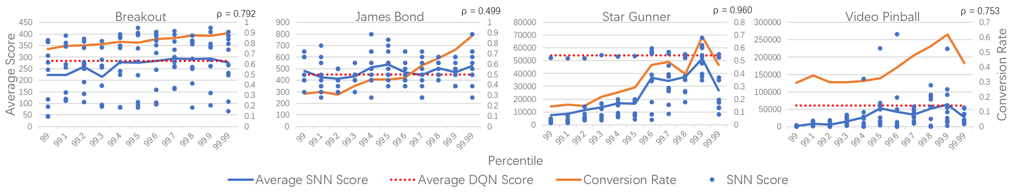
Based on the observation that there are a few activation values considerably greater than the others, which will make most of the activation values considerably less than 1, (Rueckauer et al. 2017) improves the normalization method and proposes a more robust one. Instead of using the maximum activation value of the layer to do the normalization, they use the p-th percentile activation value of the layer. P is a hyperparameter, which usually has a good performance in the range of [99.0, 99.999]. This method intends to improve the firing rate, thereby decreasing the latency until the spikes reach the deeper layers.
In the deep reinforcement learning tasks, we find the performance of the converted SNNs are very sensitive to the hyperparameter, p(percentile). It not only decreases the latency among the layers but also greatly improves the performance of the converted SNNs from DQNs. This is because by tuning the percentile, the firing rate increases, and the error caused by the leftover membrane potential is partly compensated. Thus, the accuracy gap between the original DQNs and the converted SNNs is alleviated. In this work, we make an assumption that all the spiking neurons have the same threshold. Though there are works decreasing the error by tuning the threshold in different layers separately (Sengupta et al. 2019). It actually has the same effect theoretically with changing the percentile of the parameter normalization.
Robust Firing Rate
According to equation (7), the error is inversely proportional to the simulation time. The longer simulation time we set, the smaller influence will the firing rate be affected. However, longer simulation means less power-efficient. So it is a trade-off between accuracy and efficiency. Normally the total simulation time is set to 100-1000 time steps. The firing rate is actually discrete with limited simulation time. As has been mentioned above, the q-values among different actions are very close. This makes the spiking neurons in the final layer of SNNs sometimes receive the same number of spikes, resulting in the same firing rate. This situation is particularly frequent when the simulation time is not long enough. In order to distinguish the real optimal action among spiking neurons with the same firing rate. We introduce the leftover membrane potential to solve this issue. The intuition of this method is that the neurons with higher membrane potential are more likely to generate the next spike. So when there are several neurons with the same firing rate, we should choose the neuron with the highest membrane potential. Theoretically, adding membrane potential also has its own benefit. According to equation (13), is the only part of error that we can get directly. is exactly the membrane potential at the end of the simulation time. Combining with equation (7), adding the membrane potential can eliminate the error in the last layer, which makes the firing rate of SNNs closer to the activation values of ANN.
| (17) |
where and are the firing rate and membrane potential of spiking neurons in the last layer at time t. is the proposed more robust representation of the firing rate of spiking neurons in the last layer at time . The robust firing rate not only increases the accuracy but also decreases the latency. It makes SNNs take less simulation time to distinguish the size relationships among the different actions.

Results
In this section, we use Atari games to evaluate our approach. Code used for experiments can be found at : https://github.com/WeihaoTan/bindsnet-1.
Environment
The arcade learning environment (ALE) (Bellemare et al. 2013) is a platform that provides an interface to hundreds of Atari 2600 game environments. It is designed to evaluate the development of general, domain-independent AI technology. The agent obtains the situation of the environment through image frames of the game, which is revised to 84X84 pixels, interacts with the environment with at most 18 possible actions, and receives feedback in the form of the change in the game score. Since (Mnih et al. 2015) shows human-level control of the agent on Atari games, Atari games have become a basic benchmark for deep reinforcement learning and ALE is a very popular platform for Atari games.
Without dedicated SNNs hardware, simulating firing-rate-based SNNs is a computationally demanding task, especially for reinforcement learning tasks. We choose to use BindsNET(Hazan et al. 2018) to simulate SNNs. BindsNET is the first and only open-source library used for simulating SNNs on PyTorch Platform. It takes advantage of GPUs, greatly accelerating the process of testing SNNs. All the results are run on a single NVIDIA Titan-X GPU.
Networks
To obtain the converted SNNs, we need to train DQNs first. The DQN we use is the naive DQN proposed by (Mnih et al. 2015) with 3 convolution layers and 2 fully connected layers. The first convolution layer has 32 8X8 filters with stride 4. The second convolution layer has 64 4X4 with stride 2. The third convolution layer has 64 3X3 filters with stride 1. The fully connected layer has 512 neurons. The number of neurons in the final layer depends on the number of valid actions of the tested games. We use ReLU as the activation function, which is applied to every layer except the final layer. All the games are trained with this architecture. The hyperparameters we use are also the same with (Mnih et al. 2015).
Conversion
After obtaining well-trained DQNs, we convert them to the corresponding SNNs. Firstly, we need to use IF neurons to build SNNs with the same architecture as DQNs. Before we do the parameter normalization, we need to collect the game frames to calculate the p-th maximum activation values of every layer. For each game, we collect at most 15000 frames to do the parameter normalization, then we map these parameters to the corresponding spiking neurons. Finally, we obtain the converted SNNs.
Metric
For Atari games, the score obtained in the game is the main metric to evaluate the performance of the method. However, sometimes, the average score cannot represent the performance well due to the variance if the games are not run for a sufficient number of times. To test the effect of the conversion process more efficiently and to show the result more directly, we introduce a new metric, conversion rate. It is inspired by the accuracy in image classification, and it is represented as follow:
| (18) |
where is the conversion rate, is the number of actions that the SNNs choose the same with DQNs in one game. is the total number of actions that the agent takes in the game. The conversion rate is very similar to the accuracy in the image classification task. The actions chosen by DQNs can be viewed as proxies of the correct labels. The conversion rate describes the similarity between the behavior of the SNN agent and the DQN agent. The conversion rate can be obtained by feeding the frames of the game to both the original DQN and the converted SNN simultaneously, but the agent only takes the action given by the SNN. Then we can get the conversion rate and the game score of SNN at the same time.
Testing
To test the performance of the converted SNNs, each episode of the game is evaluated up to 5 minutes (18,000 frames) per run. To test the robustness of the agent in different situations, the agent starts by random times (at most 30 times) of no-op actions. A greedy policy is applied to minimize the possibility of overfitting during the evaluation, where . If not mentioned, the firing rate we use is the robust firing rate.
| Game | DQN Score ( std) | SNN Score ( std) | Normalized SNN (% DQN) | P-Value |
|---|---|---|---|---|
| Krull | 3389667.3 | 4128.2900.4 | 121.8% | 0.0002 |
| Tutankham | 147.151.8 | 157.137.7 | 106.8% | 0.770 |
| Video Pinball | 69544.198993.2 | 74012.1129840.3 | 106.4% | 0.847 |
| Beam Rider | 8703.63648.1 | 9189.33650.4 | 105.6% | 0.522 |
| Name This Game | 8163.51394.7 | 84481457 | 103.5% | 0.596 |
| Jamesbond | 504.4127.7 | 521132.5 | 103.3% | 0.823 |
| SpaceInvaders | 2193.4927.8 | 2256.8890.4 | 102.9% | 0.932 |
| RoadRunner | 41053.66534.9 | 415885071.2 | 101.3% | 0.820 |
| Atlantis | 176044.1170037.1 | 177034 182105.7 | 100.6% | 0.760 |
| Pong | 19.91.2 | 19.81.3 | 99.7% | 0.448 |
| Kangaroo | 9874.22573.2 | 97602499.3 | 98.8% | 0.967 |
| Crazy Climber | 109885.921633.9 | 10641625946.7 | 96.8% | 0.671 |
| Tennis | 143.5 | 13.33.2 | 95.2% | 0.280 |
| Star Gunner | 57783.48202 | 546929963.3 | 94.7% | 0.038 |
| Gopher | 7076.13570.9 | 6691.23839.2 | 94.6% | 0.823 |
| Boxing | 8010.9 | 75.59.4 | 94.4% | 0.356 |
| Breakout | 311.9101.7 | 286.7117.2 | 91.9% | 0.210 |
The Effect of Simulation Time
Figure 1(a) shows the performance of SNNs with different simulation time on four games. If the simulation time is set to 100, the same frame will be fed into SNN as input for 100 times. The percentiles we choose are the ones with the best performance. From the figure, we can conclude that as the simulation time increases, the conversion rates of all the four games also increase, which is consistent with the conclusion in the Methods section that the error caused by the leftover membrane potential can be alleviated by the longer simulation time, but the effect of diminishing. It is a trade-off between the low error and the power-efficiency.
For the games that not very sensitive to the simulation time, like Breakout and James Bond, even with very short simulation time like 100 time steps, the SNN agents can still have good performance with low conversion rates. These SNN models are more robust. The error always influences the size relationships among the actions with close q-values. So the wrong actions chosen by the SNN agent can still be the sub-optimal action. The agent can still have good performance with the low conversion rate. For the games like Star Gunner and Video Pinball, these games are more sensitive to the simulation time, longer simulation time results in a larger conversion rate and then results in better performance.
The Effect of Percentile
Figure 1(b) shows the performance of SNNs with different percentile to do the parameter normalization on four games. The percentile is a very sensitive hyperparameter. Numerical studies indicate that we are unlikely to get good performance when the percentile is less than 99. Thus, we tested the effect of the percentile starting from 99. For all four games, the percentile greatly influences the conversion rate and the conversion rate affects the final score. For games like Breakout and James Bond, the conversion rate continuously improves as the percentile increases. Setting the percentile close to 100 can have good performance. For the other games like Star Gunner and Video Pinball, there is a maximum point of performance as the percentile increases. In these two games, percentile 99.9 gives the maximum value. Once exceeding this point, the performance of these games will drop dramatically. This result shows that tuning the percentile value can greatly improve the performance of the agent on these games.
The Performance of Converted SNNs on Different Games
Table 1 shows the performance of our method on multiple Atari games. Due to the limitation of resources, we choose 17 games to test the method. These are the games on which DQNs have very high performances. The total simulation time is 500 time steps. We choose the best percentile in [99.9, 99.99]. Every game is played 50 times. The average scores of DQNs and converted SNNs are shown in the table. The P-Values of DQNs and SNNs obtained by T-Test are also shown. We conclude that the scores of all SNNs are close to the scores of DQNs. And almost all the games, except Kull and Star Gunner, do not have a significant difference between DQN and SNN. This shows that the SNNs converted by our method have comparable performance to the original DQNs.
Conclusions and Future Work
This work addressed the issue of solving deep reinforcement learning problems using SNNs by converting the parameters of DQNs to SNNs.
-
•
We propose a robust conversion method, which reduces the error caused during the conversion process. We tested the proposed method on 17 Atari games and showed that SNNs can reach performances comparable with the original DQNs.
-
•
It is important to point out that our approach provides a more accurate approximation of the firing rates of spiking neurons as compared to the equivalent analog activation value proposed by (Rueckauer et al. 2017). Our work corrects some previous inaccuracies of the conversion method and further develops the theory.
-
•
To our best knowledge, our work is the first one to achieve high performance on multiple Atari games with SNNs. It paves the way to run reinforcement learning algorithms on real-time systems with dedicated hardware efficiently.
-
•
We do not have a very high conversion rate for a few games. There are some actions taken by the SNNs agent, which are not the optimal actions, which decreases the robustness of SNNs in those games. The reason for these issues is the objective of ongoing and future studies
Acknowledgments
This work has been supported in part by Defense Advanced Research Project Agency, USA Grant, DARPA/MTO HR0011-16-l-0006.
References
- Bellemare et al. (2013) Bellemare, M. G.; Naddaf, Y.; Veness, J.; and Bowling, M. 2013. The arcade learning environment: An evaluation platform for general agents. Journal of Artificial Intelligence Research 47: 253–279.
- Cao, Chen, and Khosla (2015) Cao, Y.; Chen, Y.; and Khosla, D. 2015. Spiking deep convolutional neural networks for energy-efficient object recognition. International Journal of Computer Vision 113(1): 54–66.
- Cheng et al. (2016) Cheng, H.-T.; Koc, L.; Harmsen, J.; Shaked, T.; Chandra, T.; Aradhye, H.; Anderson, G.; Corrado, G.; Chai, W.; Ispir, M.; et al. 2016. Wide & deep learning for recommender systems. In Proceedings of the 1st workshop on deep learning for recommender systems, 7–10.
- Davies et al. (2018) Davies, M.; Srinivasa, N.; Lin, T.-H.; Chinya, G.; Cao, Y.; Choday, S. H.; Dimou, G.; Joshi, P.; Imam, N.; Jain, S.; et al. 2018. Loihi: A neuromorphic manycore processor with on-chip learning. IEEE Micro 38(1): 82–99.
- Diehl et al. (2015) Diehl, P. U.; Neil, D.; Binas, J.; Cook, M.; Liu, S.-C.; and Pfeiffer, M. 2015. Fast-classifying, high-accuracy spiking deep networks through weight and threshold balancing. In 2015 International Joint Conference on Neural Networks (IJCNN), 1–8. ieee.
- Diehl et al. (2016) Diehl, P. U.; Zarrella, G.; Cassidy, A.; Pedroni, B. U.; and Neftci, E. 2016. Conversion of artificial recurrent neural networks to spiking neural networks for low-power neuromorphic hardware. In 2016 IEEE International Conference on Rebooting Computing (ICRC), 1–8. IEEE.
- Hazan et al. (2018) Hazan, H.; Saunders, D. J.; Khan, H.; Patel, D.; Sanghavi, D. T.; Siegelmann, H. T.; and Kozma, R. 2018. Bindsnet: A machine learning-oriented spiking neural networks library in python. Frontiers in neuroinformatics 12: 89.
- He et al. (2016) He, K.; Zhang, X.; Ren, S.; and Sun, J. 2016. Deep residual learning for image recognition. In Proceedings of the IEEE conference on computer vision and pattern recognition, 770–778.
- Kheradpisheh et al. (2018) Kheradpisheh, S. R.; Ganjtabesh, M.; Thorpe, S. J.; and Masquelier, T. 2018. STDP-based spiking deep convolutional neural networks for object recognition. Neural Networks 99: 56–67.
- Krizhevsky, Sutskever, and Hinton (2012) Krizhevsky, A.; Sutskever, I.; and Hinton, G. E. 2012. Imagenet classification with deep convolutional neural networks. In Advances in neural information processing systems, 1097–1105.
- LeCun, Bengio, and Hinton (2015) LeCun, Y.; Bengio, Y.; and Hinton, G. 2015. Deep learning. nature 521(7553): 436–444.
- LeCun et al. (1998) LeCun, Y.; Bottou, L.; Bengio, Y.; and Haffner, P. 1998. Gradient-based learning applied to document recognition. Proceedings of the IEEE 86(11): 2278–2324.
- Lee et al. (2020) Lee, C.; Sarwar, S. S.; Panda, P.; Srinivasan, G.; and Roy, K. 2020. Enabling spike-based backpropagation for training deep neural network architectures. Frontiers in Neuroscience 14.
- Lee, Delbruck, and Pfeiffer (2016) Lee, J. H.; Delbruck, T.; and Pfeiffer, M. 2016. Training deep spiking neural networks using backpropagation. Frontiers in neuroscience 10: 508.
- Maass and Markram (2004) Maass, W.; and Markram, H. 2004. On the computational power of circuits of spiking neurons. Journal of computer and system sciences 69(4): 593–616.
- Merolla et al. (2014) Merolla, P. A.; Arthur, J. V.; Alvarez-Icaza, R.; Cassidy, A. S.; Sawada, J.; Akopyan, F.; Jackson, B. L.; Imam, N.; Guo, C.; Nakamura, Y.; et al. 2014. A million spiking-neuron integrated circuit with a scalable communication network and interface. Science 345(6197): 668–673.
- Mnih et al. (2015) Mnih, V.; Kavukcuoglu, K.; Silver, D.; Rusu, A. A.; Veness, J.; Bellemare, M. G.; Graves, A.; Riedmiller, M.; Fidjeland, A. K.; Ostrovski, G.; et al. 2015. Human-level control through deep reinforcement learning. nature 518(7540): 529–533.
- Mozafari et al. (2018) Mozafari, M.; Ganjtabesh, M.; Nowzari-Dalini, A.; Thorpe, S. J.; and Masquelier, T. 2018. Combining stdp and reward-modulated stdp in deep convolutional spiking neural networks for digit recognition. arXiv preprint arXiv:1804.00227 1.
- Neftci et al. (2017) Neftci, E. O.; Augustine, C.; Paul, S.; and Detorakis, G. 2017. Event-driven random back-propagation: Enabling neuromorphic deep learning machines. Frontiers in neuroscience 11: 324.
- O’Connor and Welling (2016) O’Connor, P.; and Welling, M. 2016. Deep spiking networks. arXiv preprint arXiv:1602.08323 .
- Patel et al. (2019) Patel, D.; Hazan, H.; Saunders, D. J.; Siegelmann, H. T.; and Kozma, R. 2019. Improved robustness of reinforcement learning policies upon conversion to spiking neuronal network platforms applied to Atari Breakout game. Neural Networks 120: 108–115.
- Pérez-Carrasco et al. (2013) Pérez-Carrasco, J. A.; Zhao, B.; Serrano, C.; Acha, B.; Serrano-Gotarredona, T.; Chen, S.; and Linares-Barranco, B. 2013. Mapping from frame-driven to frame-free event-driven vision systems by low-rate rate coding and coincidence processing–application to feedforward ConvNets. IEEE transactions on pattern analysis and machine intelligence 35(11): 2706–2719.
- Rückauer et al. (2019) Rückauer, B.; Känzig, N.; Liu, S.-C.; Delbruck, T.; and Sandamirskaya, Y. 2019. Closing the Accuracy Gap in an Event-Based Visual Recognition Task. arXiv preprint arXiv:1906.08859 .
- Rueckauer and Liu (2018) Rueckauer, B.; and Liu, S.-C. 2018. Conversion of analog to spiking neural networks using sparse temporal coding. In 2018 IEEE International Symposium on Circuits and Systems (ISCAS), 1–5. IEEE.
- Rueckauer et al. (2017) Rueckauer, B.; Lungu, I.-A.; Hu, Y.; Pfeiffer, M.; and Liu, S.-C. 2017. Conversion of continuous-valued deep networks to efficient event-driven networks for image classification. Frontiers in neuroscience 11: 682.
- Russakovsky et al. (2015) Russakovsky, O.; Deng, J.; Su, H.; Krause, J.; Satheesh, S.; Ma, S.; Huang, Z.; Karpathy, A.; Khosla, A.; Bernstein, M.; et al. 2015. Imagenet large scale visual recognition challenge. International journal of computer vision 115(3): 211–252.
- Sengupta et al. (2019) Sengupta, A.; Ye, Y.; Wang, R.; Liu, C.; and Roy, K. 2019. Going deeper in spiking neural networks: Vgg and residual architectures. Frontiers in neuroscience 13: 95.
- Tavanaei and Maida (2019) Tavanaei, A.; and Maida, A. 2019. BP-STDP: Approximating backpropagation using spike timing dependent plasticity. Neurocomputing 330: 39–47.
- Vinyals et al. (2019) Vinyals, O.; Babuschkin, I.; Czarnecki, W. M.; Mathieu, M.; Dudzik, A.; Chung, J.; Choi, D. H.; Powell, R.; Ewalds, T.; Georgiev, P.; et al. 2019. Grandmaster level in StarCraft II using multi-agent reinforcement learning. Nature 575(7782): 350–354.
- Wu et al. (2019) Wu, Y.; Deng, L.; Li, G.; Zhu, J.; Xie, Y.; and Shi, L. 2019. Direct training for spiking neural networks: Faster, larger, better. In Proceedings of the AAAI Conference on Artificial Intelligence, volume 33, 1311–1318.
Supplymentary Material
Supplymentary Material
Table 2 shows the detailed performance of our method on 17 Atari games. The total simulation time is 500 time steps. Every game is played 50 times. We show the SNN score and conversion rate with two different percentiles, 99.9 and 99.99, which are more likely to have good performance. The SNN Score is obtained with robust firing rate. Meanwhile we also show the conversion rate of SNN using normal firing rate. From the table, we can conclude that the robust firing rate can significantly improve the conversion rate compared to the normal firing rate. And SNNs can have comparable performance compared to DQNs by tuning the percentile.
| Percentile99.9 | Percentile99.99 | ||||||
|---|---|---|---|---|---|---|---|
| Conversion Rate(%) | Conversion Rate(%) | ||||||
| Game | ANN Score | SNN Score | Normal Firing Rate | Robust Firing Rate | SNN Score | Normal Firing Rate | Robust Firing Rate |
| Atlantis | 176044.1170037.1 | 130342.0 163829.1 | 80.7 3.2 | 89.8 1.4 | 177034 182105.7 | 82.7 2.8 | 94.0 1.2 |
| Beam Rider | 8703.63648.1 | 8174.2 3457.9 | 67.0 1.1 | 73.9 1.0 | 9189.3 3650.4 | 77.7 0.9 | 90.6 0.5 |
| Boxing | 8010.9 | 78.0 20.4 | 55.6 9.8 | 57.2 10.0 | 75.5 9.4 | 76.6 4.3 | 85.8 1.9 |
| Breakout | 311.9101.7 | 286.7 117.2 | 87.0 2.9 | 87.0 1.8 | 268.2 128.9 | 89.8 2.8 | 82.9 3.6 |
| Crazy Climber | 109885.921633.9 | 92566.0 25259.3 | 42.6 3.1 | 61.4 7.3 | 106416.0 25946.7 | 45.3 3.1 | 82.5 3.1 |
| Gopher | 7076.13570.9 | 5285.6 2813.5 | 63.0 3.8 | 78.7 2.0 | 6691.2 3839.2 | 72.1 4.1 | 92.5 1.0 |
| Jamesbond | 504.4127.7 | 493.0 122.9 | 67.4 2.6 | 74.5 2.6 | 521.0 132.5 | 73.6 1.5 | 83.5 1.3 |
| Kangaroo | 9874.22573.2 | 9358.0 2408.5 | 58.4 1.5 | 70.2 1.2 | 9760.0 2499.3 | 65.7 1.7 | 87.3 0.7 |
| Krull | 3389667.3 | 4128.2 900.4 | 59.6 3.0 | 66.2 2.6 | 3697.2 758.4 | 69.5 2.2 | 80.9 1.9 |
| Name This Game | 8163.51394.7 | 8448.0 1457.0 | 53.1 1.4 | 74.1 1.3 | 8488.0 1677.9 | 56.0 1.6 | 71.6 1.4 |
| Pong | 19.91.2 | 19.4 1.5 | 59.9 1.7 | 63.9 1.7 | 19.8 1.3 | 72.0 1.8 | 85.8 1.2 |
| RoadRunner | 41053.66534.9 | 40344.0 7080.2 | 56.0 6.2 | 71.6 3.3 | 41588.0 5071.2 | 68.3 2.4 | 75.2 3.3 |
| SpaceInvaders | 2193.4927.8 | 2133.0 822.9 | 70.2 1.8 | 76.8 1.6 | 2256.8 890.4 | 70.1 1.8 | 83.0 1.6 |
| Star Gunner | 57783.48202 | 54692.0 9963.3 | 61.6 1.5 | 71.6 1.4 | 30580.0 15472.6 | 44.2 2.2 | 42.7 2.1 |
| Tennis | 143.5 | 12.2 4.3 | 59.4 1.5 | 68.0 1.0 | 13.3 3.2 | 64.8 1.7 | 72.2 1.3 |
| Tutankham | 147.151.8 | 152.0 44.3 | 88.9 6.5 | 93.4 4.7 | 157.1 37.7 | 86.2 8.6 | 97.9 1.2 |
| Video Pinball | 69544.198993.2 | 74012.1 129840.3 | 53.1 9.3 | 61.0 9.9 | 8.0 39.6 | 59.6 14.2 | 42.7 14.2 |