Strassen’s Matrix Multiplication Algorithm Is Still Faster
Abstract.
Recently, reinforcement algorithms discovered new algorithms that really jump-started a wave of excitements and a flourishing of publications. However, there is little on implementations, applications, and, especially, no absolute performance and, we show here they are not here to replace Strassen’s original fast matrix multiplication yet. We present Matrix Flow, this is a simple Python project for the automatic formulation, design, implementation, code generation, and execution of fast matrix multiplication algorithms for CPUs, using BLAS interface GPUs, and in the future other accelerators. We shall not play with module-2 () algorithms and, for simplicity, we present only square double-precision matrices. By means of factorizing the operand matrices we can express many algorithms and prove them correct. These algorithms are represented by Data Flows and matrix data partitions: a Directed Acyclic Graph. We show that Strassen’s original algorithm is still the top choice even for modern GPUs. We also address error analysis in double precision, because integer computations are correct, always.
1. Introduction
In the literature, there are quite a few algorithms for fast matrix multiplication already. For example, we used to have a few pages of references showing the rich literature. Now institutions and companies are actually stepping in and providing a complete list. Although the list of algorithms is long, the list of implementations for old and new architectures is limited in absolute terms. Here and always, we are interested in the computation with matrices, not a single elements or scalar arithmetic, and we compare the trade between matrix multiplications for pre and post matrix additions. This is important when we translate fast algorithms into practical implementations. The temporary spaces required is also an interesting aspect of the algorithm performance.
The researchers at DeepMind presented a new methodology to find new and faster matrix multiplications (PMID:36198780, ). They provide the algorithms in matrix forms and, easily, we can generate, and execute element-wise algorithms. There are new algorithms and the authors show the relative advantage performance with respect to the classic matrix multiplication for GPUs and TPUs (using XLA).
Here, we show that Strassen’s algorithm (STRASSEN1969, ) is still king of the hill. We explore a comparison across several algorithms using the standard arithmetic: double precision matrices and no modular arithmetic because it is the default in Python. Half, single and double precision, single and double complex, and also integer 8-bit can be deployed when the BLAS interface defines it for an architecture. In this scenario, we can determine a priori the relative advantages of all algorithms (i.e., 7% improvement per recursion). More interesting, we can show that deeper algorithms such as the one recently discovered do not have all the advantages when other constraints are present.
In the following, we present a Python project: Matrix Flow. Here, you can take any of the algorithms for square matrices, we use the DeepMind’s algorithms as repository, and create complex implementations you can run in CPU, GPU and in principle extend to any accelerator using the appropriate interface: we use BLAS GEMM and GEMA , these are the minimum operations for the computation in a non commutative ring. We can use also Bini’s format for the representation of the algorithms, which is our first and preferred (Paolo2007, ).
We have a few goals in mind for this work. First, we want to make available algorithms and Python implementations: both proven correct. Second, we want to provide tools for the implementation of these algorithms for highly efficient systems. Python is flexible, with such a nice abstraction level that writing code for matrix algorithms is a breeze. Efficiency and performance is not always Python forte, however writing interfaces for C/C++ is relatively simple. Interfaces are not a very good solution either and they are more a nice intermediary solution. Think of accelerators where interfaces have to change the shapes, layouts of the operands, and send them through a slow connections. So we provide tools to build entire algorithms in C/C++ for CPU and GPUs and still prove them correct and quantify rounding errors. Last, we provide tools for the validation of algorithms.
So this is a paper and a software project introduction. Here, we would like to share a few lessons learned that are not trivial, sometimes original, and important for other applications where compiler tools are designed to optimize artificial intelligence applications.
2. Matrices and Partitions.
We start by describing the non commutative ring: matrices, operations, and matrix partitions. This will help us understand and describe fast matrix multiplications constructively.
In this work we work mostly with matrices and scalar, but vector are easily added. A matrix , this is a square matrix of size . Every element of the matrix is identified by a row and a column as . A scalar is number in .
-
•
so that and these are (scalar) multiplications in .
-
•
is matrix addition and and it is commutative.
-
•
.
-
•
is matrix multiplication and , it is not commutative.
-
•
( is matrix by vector multiplication and , you will find this in the software package but it is not necessary).
Great, we have the operands and the operations. Let us introduce the last component for the description of our algorithms: Partitions. The double subscript for the definition of elements is for exposition purpose only. Here, we introduce the single subscript that in the original literature is used a lot (if not exclusively). Consider a matrix , we can consider the matrix as a composition of sub-matrices.
| (1) |
The property is that are non overlapping matrices and this is easily generalized to any factor of for example so that . For and and and :
| (2) |
Note, when we have a partition we know the matrix completely. A partition recursively applied reduces to a list of scalar elements. Let us represent the simplest matrix multiplication using partition:
| (3) |
Using the factor , we have in general
| (4) |
Equation 4, as matrix computation, represent naturally a recursive computation. Take the , we can compute it directly or partition the operands further not necessarily in the same way as in Equation 3.
A Strassen’s algorithm has the following format:
| (5) |
There are seven products, each product can be done recursively, but first we must combine submatrices of the operands accordingly to a specific set of coefficients. The coefficients and belong to three sparse matrices. Let us take the Strassen’s algorithm but represented as DeepMind would use it for the computation of Equation 5. We choose to use single subscripts for , because the notation is simpler (i.e., fewer indices), and because we implicitly use a row major layout of the sub-matrices making the single index completely determined.
| (6) |
Where the matrices , and are integer matrices with coefficients [-1,0,1], but they do not need to be integers as long the matrix stays sparse, described as follow plus some useful notations (the first column and the last row are for notations purpose only to connect to Equation 5):
| (7) |
and
| (8) |
Take matrix and consider the first row ().
| (9) |
and for better effect the last row ().
| (10) |
If we take the matrix , the columns are the products of the algorithms, in this case 7. The row explains how to sum these product so that to achieve the correct result. The matrix , each column represents the left operand of product . The matrix represent the right operand. Notice, that with the proper matrices we could achieve Equation 4
We shall use only square matrices for simplicity. Thus the key for the full determination of the Strassen algorithm is 2. This is the common factor we use to split both sides (i.e., row and column) for all matrices. If the split factor determines the algorithm with minimum number of products, so we are going to play with 2 as 7 products, 3 as 23 products, 4 as 2x2 and 49 products, 6 = 2x3 and 3x2 as 7*23 products, 9 = 3x3 as 23*23 products, 12=2x2x3, 2x3x2, 3x2x2 as 7*7*23 products.
Intuitively and if we are using the recursive idea as in Equation 5, take the algorithm with factor 6. We can take fist the factor 2, and each of the 7 products, recursively use an algorithm with factor 3 and 23 products. A pure recursive algorithm would compute the operands and first, recursively solve the result and distribute it. The sequence 2 and 3 specifies an algorithm that is different from the sequence 3 and 2. The space requirement is different: literally if we take a 6x6 matrix, if we split the matrices by 2, the temporary space to hold and are two matrices of size 3x3. The recursive call will use temporary space of size 1x1 (scalar computation). Otherwise, if we split by 3, we need a temporary space of size 2x2. The computation order is different and, even in double precision, there is a different error distribution.
Interestingly, the original problem (6x6x6), which is the complete reference in (PMID:36198780, ) splits the problem into basic products can be done using non square ones: (2x3x3) and (3x2x3). Thus, we can solve directly using a factor 6 and square matrices but with a proper factorization of , and and the order is important.
In the project there is a complete proof and a few implementations: In practice, if we use a factor 3 and we have and we have a factor 2 with , then the algorithm with factor 6 is completely defined succinctly as . Where is the Kronecker product (used also in (PMID:36198780, )). This factorization and algorithm generation is really neat: If we have a problem size that can be factorized exactly with the set of fast algorithms, then it requires just constant temporary space (last factor squared that can be just 1). We shall show application of this idea in the experimental results.
3. Matrix Flow
Take a matrix operation such as , and describe this computation by means of the matrix partitions by factors: recursively if you like by a factor of 2
| (11) |
If we use the definition of matrix multiplication to perform the computation, we can build a sequence of instructions as follows:
    ## Declarations AD single index partition of A, BD of B, CD of C
    decls = [[alphai],    AD ,        BD,          CD ]
    ###
    ## Computation as a sequence of assignment statements and binary operations.
    ###
    V = []  ## operation list
    for i in range(Row=2):
        for j in range(Col=2):
            T = Operation("p0", "*", AD[i*Col] ,BD[j])
            for k in range(1,K=2):
                T1 = Operation("p%d"%k, "*", AD[i*Col+k],BD[k*Col+j])
                T  = Operation(’c’,’+’,T,T1)
            R = Operation("s0", ’<<’,CD[i*Col+j],T)
            V.append(R)
Operation is simply an abstraction of the matrix operations and , we have only binary computations plus a constant multiplication. Such a format is standard in BLAS libraries. In practice, the declarations and the instruction sequence (i.e., V) define the computation completely. In matrix flow this is a Graph. A Graph is an extension of a function where there can be multiple inputs and outputs. Think about the factorization of a matrix into two components . A function is an extension of a matrix operation: one output and two operands.
The idea behind a graph is simple: we have clearly spelled out inputs and ouputs, we can build a clear declaration of the matrix partitions and constants, we have a list of assignment statements. The computation is summarized by a directed acyclic graph and the schedule by the sequence of instructions based on binary operators represented as an abstract syntax tree.
In the last ten years, the compiler technology for data flows computations and DAGs has had great incentives because it is the foundations of artificial intelligence applications for CPU but especially for custom accelerators (among them GPUs).
The main features of a graph in combination of using Python at the time of this writing are the following.
-
(1)
The self description of the graph is a readable code. If we create a graph using Equation 11 , the print of the graph is literally
  (Pdb) print(G1)
  CDP[0] << (ADP[0]) * (BDP[0]) + (ADP[1]) * (BDP[2])
  CDP[1] << (ADP[0]) * (BDP[1]) + (ADP[1]) * (BDP[3])
  CDP[2] << (ADP[2]) * (BDP[0]) + (ADP[3]) * (BDP[2])
  CDP[3] << (ADP[2]) * (BDP[1]) + (ADP[3]) * (BDP[3])
The symbol
<<is the assignment operation and it is overwritten instead of the Python shift operation (better than overwriting the assignment itself). -
(2)
The self description is valid Python code and it can be compiled and executed. So this is completely similar to LLVM where the graph can be explicitly encoded, the code is human readable, and it can be modified (the graph), but we can execute the code directly.
-
(3)
We can compute the graph by executing the list of operation in sequence. Can you see the list in the snippet? This is a list of operations we can evaluate sequentially. So the graph is a computational data structure. The list is one valid schedule and we can change it.
In summary, the graph is a self contained structure that can be used to execute the algorithm, to compile it, and thus validate easily. Our goal is to describe how we use this to validate correctness and relative performance of any fast algorithms and to show that by customizing the description of the graphs as code, we can generate native codes for CPU and GPU that can be easily compiled and validated in the same environment. Thus can be validated theoretically and practically. We want to focus on how we can build efficient codes especially for GPUs.
3.1. CPU and Python performance and validation
We have a systematic way to retrieve fast algorithms by factors, we can create computational graphs, for a specific problem size, and we can execute them. The first thing it is to get a feel of the performance, like in Figure 1.
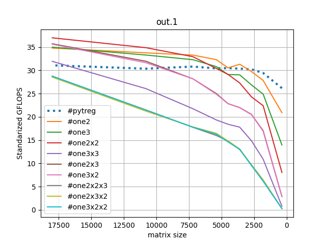
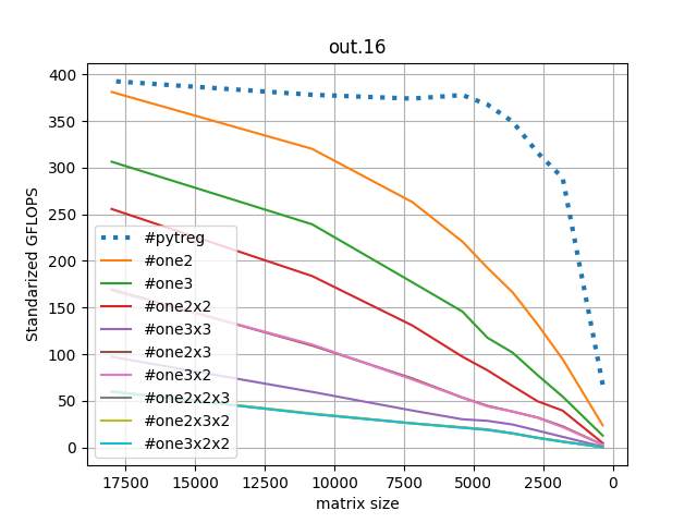
There is a lot to unpack. There are two plots, the matrix sizes go
from the largest to the smallest so we can highlight the maximum speed
up as the first spot in the graph. This is a Thread-ripper CPU with
16 cores. We can afford to give one core to the base line GEMM (and
for all fast algorithms) and we can give them 16. The first plot show
the performance when we use 1 core. The Base line is steady at 30
GFLOPS. It is clear that Strassen 2 and 2x2 (respectively,
#one2 and #one2x2) is faster for any problem size 2500
and above. All algorithms with three or more factors are behind and
they never break even but the trajectory is promising ( #one3x2x2).
The situation is different as soon as the GEMM gets more cores: In the second plot no algorithm is faster than the base line. The reason is the base line does not have a sharp increasing and, then, steady performance; that is, the performance knee between sizes 0 and 5000. In practice, the additions are constantly bad performing and the multiplications we save are small and inefficient, we are better off solving a large problem using the standard GEMM. In practice, all fast algorithms seem having slopes for which there will be no intersection or crossing for no foreseeable size.
Of course, the 16 core example is skewed towards the single call GEMM algorithm, which is never slowed down by the several function calls for each operations.
3.2. GPUs
Matrix Flow can use the same methodology to create C++ code using rocBLAS interface. In practice, we create rocBLAS calls into a single C++ package that we can compile and import in Python. Again, the interface and module idea is not efficient, it is not meant to replace any of the current implementations in C/C++/Fortran. It is just so much easier to compare and validate the correctness of the computation and report the numerical stability of the code.
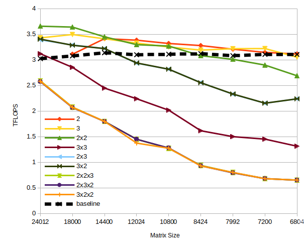
The GPU we use here is a Vega20 known as VII Radeon. The performance is for double precision and the peak performance is 3.5TFLOPS (tera = floating point per second). This GPU has a 16GB of HBM2 main memory with 1TB/s bandwidth. In Figure 2, we show the performance again from the largest to the smallest: so we can appreciate better the maximum speed up for the fast algorithms. We report kernel wall clock time that is the computation of the sequence of GEMM and GEMA without any CPU device compaction and transmission. In general, the communication between CPU and GPU takes so much more than the computation itself.
The good news is that the GPU performance is identical to the 1CORE plots (instead of the 16). Once again three factors algorithm are behind but the trajectory is pretty good they are close to break even (we did not investigate if they do because the largest problem we can execute is about 26000x26000 without leaving any space to the GEMM kernel). The 2-factor algorithms go above the baseline and Strassen 2 and 2x2 are safely in the lead.
Two caveats: the sizes we test are designed so that all algorithms have the proper factors but this does not mean that are suitable for the GEMM kernel. For the last problem size, 24012, the problem size is about 13GB (which was measured at about 80% of the VRAM available). Due to the temporary space, Strassen with factor 2, does not fit into the device (requiring about extra 3GB).
4. Conclusion
As short conclusion, in and with optimal implementation of GEMM and GEMA, deeper algorithms like the one recently found by DeepMind do not have the edge against the classic Strassen’s algorithm. If you think about it, Strassen is still pretty good.
References
- (1) A. Fawzi, M. Balog, A. Huang, T. Hubert, B. Romera-Paredes, M. Barekatain, A. Novikov, F. J. R Ruiz, J. Schrittwieser, G. Swirszcz, D. Silver, D. Hassabis, and P. Kohli, “Discovering faster matrix multiplication algorithms with reinforcement learning,” Nature, vol. 610, no. 7930, p. 47—53, October 2022. [Online]. Available: https://europepmc.org/articles/PMC9534758
- (2) V. STRASSEN, “Gaussian elimination is not optimal.” Numerische Mathematik, vol. 13, pp. 354–356, 1969. [Online]. Available: http://eudml.org/doc/131927
- (3) P. D’Alberto, “Fastmmw: Fast matrix multiplicaiton by winograd,” https://github.com/paolodalberto/FastMMW, 2013.