Strange hadron production in a quark combination model in Au+Au collisions at energies available at the BNL Relativistic Heavy Ion Collider
Abstract
We apply a quark combination model to study yield densities and transverse momentum () spectra of strange (anti-)hadrons at mid-rapidity in central Au+Au collisions at 7.7, 11.5, 19.6, 27, 39 and 200 GeV. We show that the experimental data for spectra of (anti-)hadrons in these collisions can be systematically described by the equal velocity combination of constituent quarks and antiquarks at hadronization. We obtain the spectra of quarks and antiquarks at hadronization and study their collision energy dependence. We also reproduce the yield densities of hadrons and anti-hadrons. In particular, we demonstrate that the yield ratios of anti-hadrons to hadrons , , , and simply correlate with each other and their experimental data except at 7.7 GeV are systematically described by the model. These results suggest that the equal velocity combination mechanism for quarks and antiquarks at hadronization plays an important role for the production of these long-lived hadrons in Au+Au collisions at low RHIC energies ( 11.5 GeV).
I Introduction
Hadron production from final state partons in high energy collisions is a complex Quantum Chromodynamics (QCD) process. Due to the difficulty of non-perturbative QCD, phenomenological mechanisms and models have to be applied to describe the production of hadrons at hadronization Andersson et al. (1983); Webber (1984); Das and Hwa (1977); Anisovich and Shekhter (1973); Bjorken and Farrar (1974); Xie and Liu (1988); Becattini (1996); Braun-Munzinger et al. (1996). In relativistic heavy-ion collisions at high RHIC and LHC energies, quark-gluon plasma (QGP) is created in early stage of collisions and the hadronization of QGP can be microscopically described by the quark (re-)combination/coalescence mechanism Greco et al. (2003); Fries et al. (2003); Molnar and Voloshin (2003); Lin and Molnar (2003); Shao et al. (2005); Chen and Ko (2006). The enhanced ratio of baryon to meson and number of constituent quark scaling for elliptic flows of hadrons at the intermediate transverse momentum () are typical experimental signals for quark combination mechanism at hadronization and have been widely observed in relativistic heavy-ion collisions Adare et al. (2007); Adamczyk et al. (2016a); Abelev et al. (2015); Acharya et al. (2018); Adamczyk et al. (2013); Adcox et al. (2002a); Abelev et al. (2006, 2013).
In our recent studies in high-multiplicity events in and -Pb collisions at LHC energies where the mini-QGP is possibly created and re-scattering of hadrons is weak, we found an interesting quark number scaling property for spectra of hadrons at mid-rapidity Song et al. (2017); Zhang et al. (2020). This scaling property is a direct consequence of equal velocity combination (EVC) of constituent quarks and antiquarks at hadronization. Our studies showed that the EVC of up/down, strange and charm quarks can provide a good and systematic description on spectra of light, strange and charm hadrons in ground-state in and -Pb collisions at LHC energies Song et al. (2017); Gou et al. (2017); Zhang et al. (2020); Song et al. (2018); Li et al. (2018). In latest work Song et al. (2020), we further found that the experimental data for spectra of and at mid-rapidity in heavy-ion collisions in a broad collision energy range ( GeV) also satisfy the quark number scaling property. This is a clear signal of EVC at hadronization even in heavy-ion collisions. Therefore, it is interesting to systematically test this mechanism by production of more hadron species in relativistic heavy-ion collisions.
Recently, STAR collaboration reported their precise experimental data for the production of strange hadrons in Au+Au collisions at 7.7-39 GeV Adam et al. (2020). This provides us a good opportunity to systematically study the EVC mechanism of hadron production in these collisions. In this paper, we apply a quark combination model with EVC to carry out a systematic study on yield densities and spectra of strange hadrons in Au+Au collisions at 7.7, 11.5, 19.6, 27, 39 and 200 GeV. We put particular emphasis on the self-consistency of the model in explaining the experimental data for different kinds of hadrons and on the regularity in multi-hadron production correlations which is sensitive to hadronization mechanism. Taking advantage of precise data for strange hadrons, we also study the strangeness neutralization in the midrapidity region in these collisions. We extract quark distributions at hadronization from data of hadrons and study properties of the relative abundance for strange quarks as the function of collision energy. Furthermore, we discuss the key physics in current quark combination model which are responsible for explaining successfully experimental data of hadronic spectra and yields, and discuss the creation of QGP or the deconfinement at low RHIC energies.
The paper is organized as follows. In Sec. II, we introduce a quark combination model with equal velocity combination approximation. In Sec. III, we study the strangeness neutralization in mid-rapidity region. In Sec. IV, we show results of spectra for hadrons and compare them with experimental data. In Sec. V, we study the split in yield between hadrons and their antiparticles. In Sec. VI, we study properties for the obtained numbers and spectra of quarks at hadronization at different collision energies. The summary and discussion are given at last in Sec. VII.
II A quark combination model with EVC
The quark combination is one of phenomenological mechanisms for hadron production at hadronization. The basic idea of quark combination was firstly proposed in 1970s Anisovich and Shekhter (1973); Bjorken and Farrar (1974); Das and Hwa (1977) and has many successful applications in high energy reactions Xie and Liu (1988); Buschbeck et al. (1980); Liang and Xie (1991); Braaten et al. (2002). In relativistic heavy-ion collisions, quark combination mechanism is often used to describe the hadron production at QGP hadronization Zimányi et al. (2000); Hwa and Yang (2003); Greco et al. (2003); Fries et al. (2003); Molnar and Voloshin (2003); Shao et al. (2005); Chen and Ko (2006). Recently, we found that quark combination can also well explain experimental data of hadron production in high-multiplicity and -Pb collisions at LHC energies Song et al. (2017); Gou et al. (2017); Shao et al. (2017); Zhang et al. (2020).
In this paper, inspired by the quark number scaling property of hadronic spectra Song et al. (2017); Zhang et al. (2020); Song et al. (2020), we adopt a specific version of quark combination model Song et al. (2017); Gou et al. (2017). This model assumes the combination of constituent quarks and antiquarks with equal velocity to form baryons and mesons at hadronization. The unknown non-perturbative dynamics at hadronization are parameterized and their values are assumed to be stable in high energy reactions and are fixed by experimental data. This model is essentially a statistical model based on the constituent quark degrees of freedom at hadronization and the constituent quark structure of hadrons. It is different from the popular re-combination/coalescence models which adopt the Wigner wave function method under instantaneous hadronization approximation Fries et al. (2003); Greco et al. (2003). The brief description of the model is as follows.
We start from the general formula for the production of the baryon composed of and the production of the meson composed of in quark combination mechanism
| (1) | ||||
| (2) |
Here is the joint momentum distribution for , and . The combination kernel function denotes the probability density for a given with momenta and to combine into a baryon with momentum . It is similar for mesons. We emphasize that Eqs. (1) and (2) are generally suitable for hadron production in momentum space of any dimension. In this paper, we study the one-dimensional transverse momentum () distribution of hadrons at midrapidity . In this case, simply denotes and the distribution function denotes the at midrapidity.
The combination functions and contain the key information of combination dynamics which is not clear at present due to the non-perturbative difficulty of hadronization. In our recent works Song et al. (2017); Zhang et al. (2020); Song et al. (2020), we observed an interesting quark number scaling property for the spectra of hadrons in high-multiplicity and -Pb collisions as well as in heavy-ion collisions. This scaling property supports the combination of constituent quarks and antiquarks with equal velocity. This suggests an effective form for the combination kernel functions, i.e.,
| (3) | ||||
| (4) |
Here, and are coefficients independent of momentum. Momentum fraction is determined by the masses of constituent quarks because . Specifically, we have for baryon with and for meson with . is the constituent mass for quark of flavor . Because the mass of the formed hadron under Eqs. (3) and (4) is the sum of these of constituent quarks, we take contituent masses GeV and GeV in order to properly describe the production of baryons and vector mesons studied in this paper.
The joint momentum distributions and generally contain the correlation term caused by, for example, the collective flow formed in system evolution before hadronization in heavy-ion collisions. In order to obtain analytical and simple expressions for and , we take the independent distribution approximation
| (5) | ||||
| (6) |
Substituting Eqs. (3)-(6) into Eqs. (1) and (2), we obtain
| (7) | ||||
| (8) |
and carry the information of -independent combination dynamics. In order to determine their forms, we express momentum distributions of hadrons in another form
| (9) | ||||
| (10) |
and are numbers of and , respectively. and are distribution functions normalized to one when integrating over momentum, which can be obtained by those of quarks and antiquarks,
| (11) | ||||
| (12) |
Here, is the normalized distribution function of quark . Normalization coefficients and are defined as
| (13) | ||||
| (14) |
Substituting Eqs. (11) and (12) into Eqs. (9) and (10) and then comparing them with Eqs. (7) and (8), we obtain
| (15) | ||||
| (16) |
From above two equations, we can read out the physical meaning of and . It is obvious that denotes the momentum-integrated probability of forming a baryon and denotes that of forming a meson . Two probabilities can be further decomposed as
| (17) | ||||
| (18) |
Taking meson for example, is used to denote the averaged probability of a pair forming a meson. Here, is the all possible number of pair, where is the number of all quarks and is that of all antiquarks. is the average number of mesons produced by the hadronization of quark system with given quark number and antiquark number . The factor denotes further sophisticated tune for the production probability of on the basis of the averaged probability . The baryon formula is similar to meson except a factor . This factor is to assure and equals to for with three identical flavor, two identical flavor, and three different flavors, respectively. Finally, we obtain yield formulas of hadrons
| (19) | ||||
| (20) |
and are functions of and Song and Shao (2013),
| (21) | ||||
| (22) | ||||
| (23) |
where and . Parameter denotes the production competition of baryon to meson and is tuned to be according to our recent work Shao et al. (2017).
In this paper, we only consider the production of the ground state mesons and baryons in flavor SU(3) group. In meson formation, we introduce a parameter to describe the relative weight of a quark-antiquark pair forming the state of spin 1 to that of spin 0. Here, we take in order to reproduce the measured and data in high energy reactions Adam et al. (2016); Acharya et al. (2020). Factor is then parameterized as
| (24) |
In baryon formation, we introduce a parameter to describe the relative weight of spin state to state for three quark combination. We take by fitting the experimental data of and in high energy collisions Adamova et al. (2017). Then we have for
| (25) |
except that .
Taking as model inputs, we can calculate and of hadrons directly produced at hadronization. Finally, we take the decay contribution of short-life resonances into account according to experimental measurements, and obtain results of final-state hadrons
| (26) |
where the decay function is determined by the decay kinematics and decay branch ratios Olive et al. (2014).
III Strangeness neutralization in heavy-ion collisions
In relativistic heavy-ion collisions, strange quark and antiquark are always created in pair in collisions and therefore strangeness is globally conserved. However, for a finite kinetic region such as the mid-rapidity region, the strangeness neutralization is not so explicit, in particular, at low collision energies. In this section, using the precise data for yield densities and spectra of identified hadrons Adler et al. (2004); Adams et al. (2007); Abelev et al. (2009a, b); Aggarwal et al. (2011); Adamczyk et al. (2017); Adam et al. (2020), we study the local strangeness in the midrapidity region in Au+Au collisions at STAR BES energies.
III.1 strangeness at mid-rapidity
In this subsection, we estimate strangeness density in the mid-rapidity region in relativistic heavy-ion collisions. We write for short in the following. Since experimental measurements are mainly for hadrons in ground state in flavor SU(3), we estimate the strangeness by yield densities of the following hadrons
| (27) | |||
For convenience, we use to denote . The contribution of baryons with different charge states is also abbreviated, e.g., . We note that the contribution of higher mass resonances can be effectively included if we identify above ground state hadrons as the measured ones.
The strangeness in meson sector can be calculated as
| (28) |
where we use the subscript to denote that and have received the decay contribution of . Since neutral kaons are not measured, we use the approximation
| (29) |
For strangeness contained in hyperons with one strange quark, we decompose them into two parts: experimentally measured net- and experimentally un-measured net-. Using the property of S&EM decays for hyperons Olive et al. (2014), we have
| (30) |
with
| (31) | |||
and
| (32) | |||
Applying our formula of hadronic yields in Sec. II, we obtain
| (33) |
For strangeness contained in hyperons with two strange quarks, after considering S&EM decays, we have
| (34) |
and we use the approximation
| (35) |
By the sum over the strangeness in meson and baryon sectors, we obtain the net-strangeness of the system
| (36) |
where subscript denotes the yield including S&EM decay contributions.
The total number of strange quarks and strange anti-quarks is
| (37) |
Because the strangeness is explicitly dependent on collision energies and collision centralities, we define the relative asymmetry factor
| (38) |
which is convenient to compare results in different situations.
| (GeV) | ||||||
|---|---|---|---|---|---|---|
| 200 | ||||||
| 62.4 | ||||||
| 39 | ||||||
| 27 | ||||||
| 19.6 | ||||||
| 11.5 | ||||||
| 7.7 |
In Table 1, we show results for in most central Au+Au collisions at different collisions energies 111In calculations, we use the approximation of isospin symmetry between up and down quarks in Eqs. (29) and (35). If we consider the small asymmetry in number between up quarks and down quarks coming from colliding nucleons, we should modify Eq. (29) by multiplying a factor and Eq. (35) by multiplying a factor in right hand side of equation and the corresponding coefficients in Eqs. (36) and (37). According to the number of newborn quarks extracted in next section and net-quarks from participant nucleons, we obtain, for example, at 200 GeV and at 7.7 GeV. The resulting are (-0.004, -0.018, -0.0014, -0.005, 0.002, 0.003, -0.009) at (200, 62.4, 39, 27, 19.6, 11.5, 7.7) GeV, respectively. They are very close to those shown in Tab. 1. Experimental data for yield densities of hadrons that are used in calculation are also presented Adler et al. (2004); Adams et al. (2007); Abelev et al. (2009a) Abelev et al. (2009b); Aggarwal et al. (2011); Abelev et al. (2009a) Adamczyk et al. (2016b); Adam et al. (2020). Because some data for and are results in 0-10% centrality, we re-scale them by multiplying a factor according to the participant nucleon number . We do the similar re-scaling for data of in 0-60% centrality at 7.7 GeV. Because data of and mesons are usually absent, we neglect them and therefore the calculated is over-estimated. We see that at seven collision energies are quite small. Therefore, strangeness neutralization is well satisfied in mid-rapidity region in heavy-ion collisions at RHIC energies.
III.2 spectrum symmetry
In this subsection, we study the symmetry property between spectrum of strange quark and that of strange antiquark . For this purpose, we choose () which consists of only strange quarks (antiquarks). Using Eq. (7), we have
| (39) | ||||
| (40) |
from which we have
| (41) |
where is independent of but is dependent on quark numbers. We emphasize that is not equal to one at nonzero net quark number.

Using data of spectra for and in central Au+Au collisions Adamczyk et al. (2016b); Adam et al. (2020), we calculate the ratio at different collision energies and present results in Fig. 1. Since we have shown in the previous subsection, we multiply a proper constant before data of to satisfy and therefore we can directly compare in/at different collision centralities/energies. Because of finite statistics of and , data points of show a certain fluctuations around one. On the whole, we can see that is a good approximation at the studied collision energies.
IV spectra of hadrons
In this section, we use the quark combination model (QCM) in Sec. II to study spectra of light-flavor hadrons in Au+Au collisions at RHIC energies. The inputs of model are spectra of quarks and antiquarks at hadronization. Here, we take based on the study of strangeness neutralization in Sec. III. We take for the newborn up and down anti-quarks. Because a part of up and down quarks comes from the colliding nucleons, spectrum of up quarks is not exactly the same as that of down quarks. As discussed in [47], the relative difference in number between up and down quarks is only a few percentages. We have checked that spectra of hadrons and yield ratios of anti-hadron to hadron studied in this paper are not sensitive to this small asymmetry. Therefore, in this paper, we take the approximation in the mid-rapidity region.
In Table 2, we list all inputs and parameters of the model which are needed to calculate spectra of hadrons. As introduced in model description in Sec. II, two parameters and are taken as 0.55 and 0.5, respectively, at all the studied collision energies. For three inputs, is fixed by using our model to fit experimental data of , and () is fixed by experimental data of (anti-)baryons containing such as (anti-)proton Abelev et al. (2009b); Adamczyk et al. (2017, 2016b), respectively. The extracted results for quark spectra in Au+Au collisions for 0-5% centrality at six RHIC energies are shown in Fig. 2.
| input | parameter | |||
|---|---|---|---|---|


In Fig. 3, we show the calculated results for spectra of hadrons in central Au+Au collisions at 200 GeV and compare them with experimental data Abelev et al. (2006); Adams et al. (2007); Abelev et al. (2009a). We see that the agreement between our model results and experimental data is satisfactory. Although there exists many successful explanations on these experimental data in the framework of quark combination mechanism in previous works Fries et al. (2003); Greco et al. (2003); Hwa and Yang (2003); Chen and Ko (2006); Shao et al. (2005, 2009), here we would like to emphasize that the current EVC model can systematically explain these data in a simple way. Furthermore, the good agreement at top RHIC energy provides important basis for the application of our model to lower RHIC energies.
In Figs. 4, 5, 6, 7 and 8, we show results for spectra of hadrons in central Au+Au collisions at 39, 27, 19.6, 11.5 and 7.7 GeV and compare with experimental data Adamczyk et al. (2016b, 2017); Adam et al. (2020). At 39, 27, 19.6, 11.5 GeV, we see a good agreement between our model results and experimental data Adamczyk et al. (2016b, 2017); Adam et al. (2020). In particular, we see that experimental data for baryons (, , , ) and meson can be explained by the model very well. At 7.7 GeV, we also see that model results are in good agreement with available experimental data. However, compared with data in Figs. 3-7, the available data at 7.7 GeV cover smaller range and data in the most central collisions are absent. Therefore the comparison at 7.7 GeV is not as conclusive as those at other five higher energies. We should study this energy point further in the future when more precise data are available.
Using these systematic calculations and comparisons, we would like to emphasize the equal-velocity combination of quarks and antiquarks as the effective description at hadronization. This is manifested by the following two points. First, from panel (d) in Figs. 3-7, we see that experimental data of and can be perfectly explained by the same in a very simple way,
| (42) | ||||
| (43) |
We call this property as the quark number scaling for hadronic spectra. We have shown that this property not only exists in relativistic heavy-ion collisions but also exists in high-multiplicity and -Pb collisions at LHC energies Song et al. (2017); Zhang et al. (2020); Song et al. (2020). Second, we see that data of and can be simultaneously explained by from and from proton,
| (44) | ||||
| (45) |
after further including the decay contribution of heavier baryons. Here, . This is a clear support for the equal-velocity combination for quarks with different flavors.
V Hadronic yields and multi-particle correlations
In this section, we study the -integrated yields of identified hadrons. In heavy-ion collisions at RHIC energies, the net baryon numbers deposited in the mid-rapidity region will influence the production of hadrons and antihadrons to a certain extent. One of the consequences for non-zero baryon number density is the asymmetry in yield between hadrons and their anti-particles. We study this yield asymmetry with our model by focusing on multi-particle yield correlations.
In Fig. 9, we show yield densities of hadrons and anti-hadrons 222Model results for yield densities of kaons are presented here. Because the direct combination in the current EVC model has energy conservation issue, we have to introduce further treatment to reconcile this such as we did in Ref. Gou et al. (2017). However, the strange quantum number conservation ensures that the number of the formed kaon can be correctly calculated in the current model. divided by participant nucleon number at mid-rapidity in central Au+Au collisions at different collision energies. Open symbols are experimental data Adams et al. (2004, 2007); Abelev et al. (2009b); Aggarwal et al. (2011); Adamczyk et al. (2017); Adam et al. (2020); Adcox et al. (2002b) and solid symbols are model results. Experimental data show that the yield split between and in (a) is much smaller than that between and in (b). Yield split between and in (c) and that between and in (d) are larger than kaon split in (a) but are smaller than proton split in (b). Comparing with experimental data, we see that the model provides a globally good description for yield densities of hadrons and anti-hadrons.

In order to further study the split in yield between hadrons and anti-hadrons, we calculate the ratio of yield for anti-hadron to that for hadron. Yield ratio is not sensitive to the numbers of quarks and antiquarks at hadronization and is also not sensitive to some hadronization details such as parameters and introduced in our model. Therefore, it can be used to provide a more direct test for the quark combination mechanism at hadronization in relativistic heavy-ion collisions. Experimentally measured protons and anti-protons contain complex decay contributions of heavier baryons and anti-baryons,
| (46) |
where we use the particle name with superscript to denote the yield density of final-state hadron receiving the decay contributions and the particle name without superscript in the right hand side of the equation to denote yields of directly-produced hadrons by hadronization. The ratio finally behaves as
| (47) |
where is net-quark fraction and the factor is related to the baryon-meson production competition Song and Shao (2013); Shao et al. (2017), see Eq. (23) and texts below. For yields of kaons, we take the decay contributions of and into account and have
| (48) |
where .
For yields of , and their anti-particles, we consider the S&EM decay contributions,
| (49) |
and
| (50) |
For , we directly have
| (51) |
In Eqs. (48-50), the power term dominates the behavior of three ratios. Therefore, ratios , , , and in our model are simply correlated with each other by the net-quark fraction .
Based on Eqs. (47-51), we can build several multi-hadron correlations as more sensitive tests of quark combination mechanism. In Fig. 10 (a), we firstly show the correlation between and . This correlation shows how the production of baryon and that of meson in heavy-ion collisions are simultaneously influenced by the baryon quantum number density characterized by net-quark fraction in our model. Symbols are experimental data at mid-rapidity in central and semi-central collisions Adcox et al. (2002b); Adams et al. (2004, 2007); Abelev et al. (2009b); Arsene et al. (2010); Aggarwal et al. (2011); Adamczyk et al. (2017); Adam et al. (2020). Error bars are the quadratic sum of statistical and systematic uncertainties. The dashed line is the result of QCM by Eqs. (47) and (48). Different from our previous work Song and Shao (2013) and previous experimental measurements Arsene et al. (2010), here we show the correlation in double-logarithmic coordinates in order to provide a full and clear presentation because ratio changes much faster than . We see that experimental data in double-logarithmic coordinates behave as almost a straight line and our model can well reproduce this correlation.
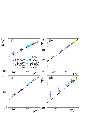
In Fig. 10 (b) we show the correlation between and . We see that experimental data, symbols in the figure, exhibit a linear behavior in double-logarithmic coordinates. This behavior can be perfectly reproduced in our model by Eqs. (47) and (49), see the dashed line. In addition, we note that ratio decreases slower than by a factor . This is because that, compared with , ratio involves a strangeness neutralization
In Fig. 10 (c) we show the correlation between and . Experimental data also exhibit a linear behavior in double-logarithmic coordinates. Since involves double effect of strangeness neutralization , decreases slower than as the function of . Our model result Eqs. (47) and (50), the dashed line in the figure, can well describe data at 11.5 GeV and slightly under-estimates at 7.7 GeV.
In Fig. 10 (d), we further show the correlation among mutl-strangeness hadrons and . Experimental data in double-logarithmic coordinates also exhibit a linear behavior. Because ( ) completely consists of strange (anti)quarks, ratio involves triple effect of strangeness neutralization and therefore it decreases slower than . The model result by Eqs. (50) and (51), the dashed line in the figure, can roughly describe data at 11.5 GeV and under-estimates at 7.7 GeV to a certain extent.
Some discussions on above results are necessary. First, we emphasize the key physics in our model relating to multi-hadron correlations shown in Fig. 10. As shown by Eqs. (47)-(51), correlations among yield ratios of anti-hadron to hadron are not sensitive to absolute numbers of quarks and antiquarks at hadronization and non-perturbative parameters and introduced in the model. Therefore, these yield correlations are only related to two basic features of quark combination in our model. (1) free combination. Newborn quarks and antiquarks, net-quarks are all treated as individual (anti-)quarks and freely take part in combination. (2) flavor independent combination probability. We take as the averaged probability of forming a baryon and as the averaged probability of forming a meson. No sophisticated flavor correction is made at the moment. From Fig. 10, we see that such a global quark combination model provides a systematic description on multi-hadron yield correlations in Au+Au collisions, at least at 11.5 GeV. Therefore, this is a clear signal of quark combination mechanism at hadronization in these collisions.
Second, the comparison between our model calculation and experimental data in Au+Au collisions at 7.7 GeV may indicate some physics beyond the key features of quark combination discussed above. As and ratios are reproduced, we see that model results for ,and are smaller than experimental data to a certain extent. This may be related to the point (1) discussed above. In Au+Au collisions at low energy, the colliding nucleons may not break completely. A part of nucleon fragments may do not behave as the individual up/down quarks and freely take part in the combination with newborn quarks and antiquarks; Instead, they behave as diquarks and can form proton by combining with a up/down quark or form by combining with a strange quark. Because these net-quarks only contribute to proton and production, net-quark fraction used in Eqs. (48), (50) and (51) for , and should be smaller than that in and . This consideration can increase ratios , and at the given and ratios and therefore can qualitatively improve the description at 7.7 GeV in the current model. Such a sophisticated effect of net-quarks is worthwhile to be studied in detail in the future works.
VI properties of quark distributions
By studying experimental data of hadronic spectra, we have obtained spectra of quarks at hadronization, which are shown in Fig. 2. In this section, we study properties of these obtained quark distributions at hadronization.
We firstly calculate the ratio and study its dependence. Fig. 11 shows results in central Au+Au collisions at 200, 39, 27, 19.6 and 11.5 GeV. Result of in collisions at TeV Zhang et al. (2020) is also presented. We see that ratios in Au+Au collisions are obviously higher than that in collisions. This means that the production of strange quarks in the studied range in Au+Au collisions is significantly enhanced. In addition, we see that ratios in Au+Au collisions at these collision energies in the low range ( GeV/c) all increase with . It is similar to results. This property is related to the complex (non-)perturbative QCD evolution in connection with quark masses in partonic phase.

We note that the increase of the ratio at low in heavy-ion collisions can be qualitatively understood by thermal statistics. In the case of thermal equilibrium such as the Boltzmann distribution in two-dimensional transverse momentum space, heavier mass will lead to flatter shape of the distribution and thus lead to the increase of the ratio. However, Boltzmann distribution at hadronization temperature in the rest frame can not directly describe the obtained quark distributions in Fig. 2. We should further take into account the contribution of the collective radial flow in the prior partonic phase evolution in heavy-ion collisions. As an illustration, we consider a simple situation, that is, Boltzmann distribution in the two-dimensional transverse momentum space boosted with a radial flow velocity . In this case the distribution is
| (52) |
with and . If we assume that quarks of different flavors at hadronization are thermalized and boosted with the same radial velocity, we can use the above formula to simultaneously describe the extracted and in the low range ( GeV/c) in Fig. 2. According to our previous work Song et al. (2020), the hadronization temperature is taken as (0.164, 0.163, 0.162, 0.161, 0.156) GeV in central Au+Au collisions at (200, 39, 27, 19.6, 11.5) GeV, respectively. We obtain radial flow velocity (0.39, 0.28, 0.27, 0.25, 0.23) at these collision energies.
We find that these results for radial flow velocity are consistent with our previous extraction by a hydrodynamics-motivated blast-wave model Schnedermann et al. (1993) fit of with the same hadronization temperature Song et al. (2020). We also find that and extracted in this work can also be consistently described in blast-wave mode. Here, taking central Au+Au collisions at 19.6 GeV as an example, we show in Fig. 12 (a) the fit results of quark spectra by Eq. (52) and those by blast-wave model at the same hadronization temperature 0.161 GeV and radial flow velocity 0.25 . We see that two fit methods give the consistent description on quark spectra. In addition, we see from Fig. 12 (b) that the increase part of the ratio in the low range can be reasonably described.

Fig. 11 also shows the ratio globally increases with the decrease of collision energies. To study this energy dependence of strangeness, we calculate the strangeness factor
| (53) |
and present results in Fig. 13. Here, results of in central Au+Au collisions at 62.4 and 130 GeV are also shown. The uncertainty of is caused by that of experimental data for yield ratios such as , , . We note that these new results of are consistent with our previous works Shao et al. (2009); Sun et al. (2012); Shao et al. (2015). Compared with in elementary collisions such as and reactions, we see that in heavy-ion collisions is obviously enhanced. We also see that increases as the decrease of collision energy.

The dependence of on collision energy is related to the varied baryon quantum number density. In this paper, we study this energy dependence in the framework of thermodynamics for quark system. We consider a thermal system consisting of constituent quarks and antiquarks. In our quark combination model, constituent quarks and antiquarks are regarded as the effective degrees of freedom at hadronization and they freely combine into baryons and/or mesons at hadronization. Therefore, we can treat such a constituent quark system as the classical gas.
Because we study the production of hadrons in mid-rapidity range, we firstly discuss the case of grand-canonical ensemble. The number of quark under Fermi-Dirac statistics in the grand-canonical ensemble is
| (54) |
where is system volume and is temperature. is degeneracy factor of quark, is quark mass and is chemical potential of quark . is the modified Bessel function of the second kind. As discussions of local strangeness conservation in Sec. III, we set to get . We assume the iso-spin symmetry between up and down quarks, then we have . Then, the strangeness factor in grand-canonical ensemble (GCE) of free quark gas is
| (55) |
In the second line, we consider only the leading term , which is corresponding to the Boltzmann statistics. As we know, baryon chemical potential is increased as the decrease of the collision energy. Therefore, the collision energy dependence of is qualitatively understood.
For a demonstrative calculation for the collision energy dependence of , we first apply Eq. (55) with the re-tuned GeV and GeV to give a proper strangeness at vanishing baryon chemical potential . Then, we apply Eq. (54) to fit the total quark number and net-quark number integrated from Fig. 2 and obtain and of quark system at hadronization. Here, the hadronization temperature is taken as before. Then we substitute and into Eq. (55). The calculated results for at RHIC energies are shown as triangles with the dashed line in Fig. 13. We see that the extracted in quark combination model can be explained by grand-canonical ensemble of quark gas system at GeV. At lower two collision energies, GCE results are higher than our extraction.
Considering the longitudinal rapidity space of heavy-ion collisions is finite, in particular, at GeV, the studied mid-rapidity range is not a tiny fraction of the whole system, the hadron production in the midrapidity range may be influenced by effects of global charge conservation not only strangeness conservation but also baryon quantum number conservation. Therefore, grand-canonical treatment may be not perfectly suitable. We now consider the result of canonical ensemble for free quark system. We apply the method of canonical statistics Becattini and Ferroni (2004) to obtain the property of quark number distribution under the constraint of finite baryon quantum number and strangeness. We put the detailed derivation into Appendix A. The inputs of canonical ensemble are volume , temperature , and charges (,,). The temperature is set to the hadronization temperature whose values at different collision energies are taken as before. As discussions in Sec. III, we take . , and can be determined by fitting the quark and antiquark numbers integrated from Fig. 2. Results of for canonical ensemble of quark system are shown as solid circles with the dotted line in Fig. 13. We see that is also increased with the decrease of collision energy and is smaller than , in particular, at low collision energies. Our extracted is roughly located in the middle of two ensembles.
VII Summary and discussions
In this paper, we have applied a quark combination model with equal-velocity combination approximation to systematically study the production of hadrons in Au+Au collisions at RHIC energies. The model applied in this work is motivated by our recent findings for the constituent quark number scaling property of hadronic spectra in high energy , A and AA collisions Song et al. (2017); Zhang et al. (2020); Song et al. (2020). After systematic study of spectra and yields for hadrons, we found that our quark combination model provides a good explanation on the experimental data in Au+Au collisions at GeV. This suggests that the constituent quark degrees of freedom still play important role even at low RHIC energy, which is closely related to the deconfinement at these collision energies.
By study of hadronic spectra and yields in these collisions, we obtained spectra and numbers of constituent quarks and antiquarks at hadronization. We calculated the net strangeness at mid-rapidity and showed the strangeness neutralization is well satisfied at mid-rapidity in heavy-ion collisions at RHIC energies. We studied the spectrum ratio of strange quarks to newborn up/down quarks and the integrated number ratio at different collision energies. We applied the basic thermal statistics for free constituent quark system to understand these properties of strange quarks relative to up/down quarks.
We emphasize the key physics in our model which are responsible for successfully explaining experimental data of hadronic spectra and yields. First, the model takes the constituent quarks and antiquarks as the effective interface connecting the strongly-interacting system before hadronization and that after hadronization. We assume the constituent quarks and antiquarks as effective degrees of freedom for the strongly-interacting quark-gluon system just before hadronization. On the other hand, we take the constituent quark model to describe the static structure of hadrons in the ground state. In this scenario, the equal-velocity combination of these constituent quarks and antiquarks is a reasonable approximation and is indeed supported by the quark number scaling property for spectra of hadrons observed in experiments Song et al. (2017); Zhang et al. (2020); Song et al. (2020). The study in this paper further showed that the equal-velocity combination can systematically describe the production of different kinds of hadrons in heavy-ion collisions at RHIC energies. Second, the model includes reasonable considerations for the unity of hadronization and the linear response property, see detailed discussions in Song and Shao (2013). This is very important to reproduce the multi-hadron yield correlations shown in Fig. 10. For example, in a naive inclusive view of combination, we have and and therefore which is independent of collision energy. However, yield of in our model is not only dependent on but also dependent on the global system information shown as in Eq. (17); thus we have in Eq. (51) which decreases with the decrease of collision energy.
In order to further test our EVC model, the following two aspects are deserved to study in depth in future works. The first is the effect of momentum correlations among quarks and antiquarks at hadronization. It is neglected in this paper, see Eqs. (5) and (6). In general, quarks and antiquarks at hadronization always have some momentum correlations. In heavy-ion collisions, the collective flow formed in parton phase will cause a certain correlation among momenta of quarks and antiquarks. This correlation not only influences the inclusive momentum spectra of hadrons to a certain extent but also influences multi-particle momentum correlations more directly. In the future work, we will study this effect by building sensitive physical observables in EVC model. The second is the production of short-lived resonances. In heavy-ion collisions, yield and momentum spectra of finally-observed resonances such as are strongly influenced by re-scatterings among hadrons. In the future work, we will systematically consider this hadronic rescattering effect and study the production mechanism of the short-lived resonances at hadronization.
VIII Acknowledgments
This work is supported in part by the National Natural Science Foundation of China under Grant No. 11975011, Shandong Province Natural Science Foundation under Grant Nos. ZR2019YQ06 and ZR2019MA053, and Higher Educational Youth Innovation Science and Technology Program of Shandong Province (2019KJJ010, 2020KJJ004).
Appendix A Quark number distribution in canonical ensemble
The probability of a single state in the canonical ensemble is
| (56) |
where is the inverse temperature, is the energy of the state and are abelian charges of the state
| (57) |
Here is the number of particle in the current state and is the quantum number vector for the -th particle. is the number of particle species.
The multiplicity distribution of particles can be obtained from the generating function associated to the canonical partition function Becattini and Ferroni (2004) and is expressed as
| (58) | |||
where the summation takes different configurations for into account under the condition .
| (59) |
Now, we consider the thermal system consisting of constituent quarks and antiquarks. In our quark combination model, constituent quarks and antiquarks are regarded as the effective degrees of freedom at hadronization and they freely combine to form baryons and/or mesons at hadronization. Therefore, we can simply apply above formula to obtain the number distribution of these “free” constituent quarks and antiquarks under canonical statistics. Here, we consider up, down, strange quarks and their antiparticles. Index denotes , and .
Eq. (58) can be further denoted as
| (60) |
where is cycle-index polynomial of symmetric group. can be numerically evaluated using the recurrence relation
| (61) |
with and .
As discussed in Sec. III, we take strangeness neutralization and therefore . For constraints of baryon charge and electric charge , we denote them as and . Finally the joint distribution function of quark numbers and antiquark numbers is
| (62) |
We obtain the averaged number of quarks by
| (63) | ||||
| (64) |
and calculate strangeness factor in canonical ensemble of free quark system.
References
- Andersson et al. (1983) B. Andersson, G. Gustafson, G. Ingelman, and T. Sjostrand, Phys. Rept. 97, 31 (1983).
- Webber (1984) B. Webber, Nucl. Phys. B 238, 492 (1984).
- Das and Hwa (1977) K. P. Das and R. C. Hwa, Phys. Lett. 68B, 459 (1977), [Erratum: Phys. Lett.73B,504(1978)].
- Anisovich and Shekhter (1973) V. Anisovich and V. Shekhter, Nucl. Phys. B 55, 455 (1973), [Erratum: Nucl.Phys.B 63, 542–542 (1973)].
- Bjorken and Farrar (1974) J. D. Bjorken and G. R. Farrar, Phys. Rev. D9, 1449 (1974).
- Xie and Liu (1988) Q.-B. Xie and X.-M. Liu, Phys. Rev. D38, 2169 (1988).
- Becattini (1996) F. Becattini, Z. Phys. C 69, 485 (1996).
- Braun-Munzinger et al. (1996) P. Braun-Munzinger, J. Stachel, J. Wessels, and N. Xu, Phys. Lett. B 365, 1 (1996), arXiv:nucl-th/9508020 .
- Greco et al. (2003) V. Greco, C. M. Ko, and P. Lévai, Phys. Rev. Lett. 90, 202302 (2003), arXiv:nucl-th/0301093 [nucl-th] .
- Fries et al. (2003) R. J. Fries, B. Müller, C. Nonaka, and S. A. Bass, Phys. Rev. Lett. 90, 202303 (2003), arXiv:nucl-th/0301087 [nucl-th] .
- Molnar and Voloshin (2003) D. Molnar and S. A. Voloshin, Phys. Rev. Lett. 91, 092301 (2003), arXiv:nucl-th/0302014 [nucl-th] .
- Lin and Molnar (2003) Z.-w. Lin and D. Molnar, Phys. Rev. C 68, 044901 (2003), arXiv:nucl-th/0304045 .
- Shao et al. (2005) F.-l. Shao, Q.-b. Xie, and Q. Wang, Phys. Rev. C71, 044903 (2005), arXiv:nucl-th/0409018 [nucl-th] .
- Chen and Ko (2006) L.-W. Chen and C. M. Ko, Phys. Rev. C73, 044903 (2006), arXiv:nucl-th/0602025 [nucl-th] .
- Adare et al. (2007) A. Adare et al. (PHENIX), Phys. Rev. Lett. 98, 162301 (2007), arXiv:nucl-ex/0608033 [nucl-ex] .
- Adamczyk et al. (2016a) L. Adamczyk et al. (STAR), Phys. Rev. Lett. 116, 062301 (2016a), arXiv:1507.05247 [nucl-ex] .
- Abelev et al. (2015) B. B. Abelev et al. (ALICE), JHEP 06, 190 (2015), arXiv:1405.4632 [nucl-ex] .
- Acharya et al. (2018) S. Acharya et al. (ALICE), JHEP 09, 006 (2018), arXiv:1805.04390 [nucl-ex] .
- Adamczyk et al. (2013) L. Adamczyk et al. (STAR), Phys. Rev. C88, 014902 (2013), arXiv:1301.2348 [nucl-ex] .
- Adcox et al. (2002a) K. Adcox et al. (PHENIX), Phys. Rev. Lett. 88, 242301 (2002a), arXiv:nucl-ex/0112006 .
- Abelev et al. (2006) B. Abelev et al. (STAR), Phys. Rev. Lett. 97, 152301 (2006), arXiv:nucl-ex/0606003 .
- Abelev et al. (2013) B. B. Abelev et al. (ALICE), Phys. Rev. Lett. 111, 222301 (2013), arXiv:1307.5530 [nucl-ex] .
- Song et al. (2017) J. Song, X.-r. Gou, F.-l. Shao, and Z.-T. Liang, Phys. Lett. B774, 516 (2017), arXiv:1707.03949 [hep-ph] .
- Zhang et al. (2020) J.-w. Zhang, H.-h. Li, F.-l. Shao, and J. Song, Chin. Phys. C44, 014101 (2020), arXiv:1811.00975 [hep-ph] .
- Gou et al. (2017) X.-r. Gou, F.-l. Shao, R.-q. Wang, H.-h. Li, and J. Song, Phys. Rev. D96, 094010 (2017), arXiv:1707.06906 [hep-ph] .
- Song et al. (2018) J. Song, H.-h. Li, and F.-l. Shao, Eur. Phys. J. C78, 344 (2018), arXiv:1801.09402 [hep-ph] .
- Li et al. (2018) H.-H. Li, F.-L. Shao, J. Song, and R.-Q. Wang, Phys. Rev. C97, 064915 (2018), arXiv:1712.08921 [hep-ph] .
- Song et al. (2020) J. Song, F.-l. Shao, and Z.-t. Liang, Phys. Rev. C 102, 014911 (2020), arXiv:1911.01152 [nucl-th] .
- Adam et al. (2020) J. Adam et al. (STAR), Phys. Rev. C 102, 034909 (2020), arXiv:1906.03732 [nucl-ex] .
- Buschbeck et al. (1980) B. Buschbeck, H. Dibon, and H. R. Gerhold, Z. Phys. C7, 73 (1980).
- Liang and Xie (1991) Z.-T. Liang and Q.-B. Xie, Phys. Rev. D 43, 751 (1991).
- Braaten et al. (2002) E. Braaten, Y. Jia, and T. Mehen, Phys. Rev. Lett. 89, 122002 (2002), arXiv:hep-ph/0205149 [hep-ph] .
- Zimányi et al. (2000) J. Zimányi, T. S. Biró, T. Csörgő, and P. Lévai, Phys. Lett. B472, 243 (2000), arXiv:hep-ph/9904501 [hep-ph] .
- Hwa and Yang (2003) R. C. Hwa and C. B. Yang, Phys. Rev. C67, 034902 (2003), arXiv:nucl-th/0211010 [nucl-th] .
- Shao et al. (2017) F.-l. Shao, G.-j. Wang, R.-q. Wang, H.-h. Li, and J. Song, Phys. Rev. C 95, 064911 (2017), arXiv:1703.05862 [hep-ph] .
- Song and Shao (2013) J. Song and F.-l. Shao, Phys. Rev. C 88, 027901 (2013), arXiv:1303.1231 [nucl-th] .
- Adam et al. (2016) J. Adam et al. (ALICE), Eur. Phys. J. C76, 245 (2016), arXiv:1601.07868 [nucl-ex] .
- Acharya et al. (2020) S. Acharya et al. (ALICE), Phys. Lett. B 807, 135501 (2020), arXiv:1910.14397 [nucl-ex] .
- Adamova et al. (2017) D. Adamova et al. (ALICE), Eur. Phys. J. C77, 389 (2017), arXiv:1701.07797 [nucl-ex] .
- Olive et al. (2014) K. Olive et al. (Particle Data Group), Chin. Phys. C 38, 090001 (2014).
- Adler et al. (2004) S. S. Adler et al. (PHENIX), Phys. Rev. C69, 034909 (2004), arXiv:nucl-ex/0307022 [nucl-ex] .
- Adams et al. (2007) J. Adams et al. (STAR), Phys. Rev. Lett. 98, 062301 (2007), arXiv:nucl-ex/0606014 [nucl-ex] .
- Abelev et al. (2009a) B. I. Abelev et al. (STAR), Phys. Rev. C79, 064903 (2009a), arXiv:0809.4737 [nucl-ex] .
- Abelev et al. (2009b) B. I. Abelev et al. (STAR), Phys. Rev. C79, 034909 (2009b), arXiv:0808.2041 [nucl-ex] .
- Aggarwal et al. (2011) M. M. Aggarwal et al. (STAR), Phys. Rev. C83, 024901 (2011), arXiv:1010.0142 [nucl-ex] .
- Adamczyk et al. (2017) L. Adamczyk et al. (STAR), Phys. Rev. C96, 044904 (2017), arXiv:1701.07065 [nucl-ex] .
- Adamczyk et al. (2016b) L. Adamczyk et al. (STAR), Phys. Rev. C 93, 021903 (2016b), arXiv:1506.07605 [nucl-ex] .
- Shao et al. (2009) C.-e. Shao, J. Song, F.-l. Shao, and Q.-b. Xie, Phys. Rev. C80, 014909 (2009), arXiv:0902.2435 [hep-ph] .
- Adams et al. (2004) J. Adams et al. (STAR), Phys. Rev. Lett. 92, 182301 (2004), arXiv:nucl-ex/0307024 .
- Adcox et al. (2002b) K. Adcox et al. (PHENIX), Phys. Rev. Lett. 89, 092302 (2002b), arXiv:nucl-ex/0204007 .
- Arsene et al. (2010) I. Arsene et al. (BRAHMS), Phys. Lett. B 687, 36 (2010), arXiv:0911.2586 [nucl-ex] .
- Schnedermann et al. (1993) E. Schnedermann, J. Sollfrank, and U. W. Heinz, Phys. Rev. C48, 2462 (1993), arXiv:nucl-th/9307020 [nucl-th] .
- Sun et al. (2012) L.-X. Sun, R.-Q. Wang, J. Song, and F.-L. Shao, Chin. Phys. C 36, 55 (2012), arXiv:1105.0577 [hep-ph] .
- Shao et al. (2015) F.-l. Shao, J. Song, and R.-q. Wang, Phys. Rev. C92, 044913 (2015), arXiv:1505.03010 [hep-ph] .
- Becattini and Ferroni (2004) F. Becattini and L. Ferroni, Eur. Phys. J. C 38, 225 (2004), [Erratum: Eur.Phys.J. 66, 341 (2010)], arXiv:hep-ph/0407117 .