Stochastic Thermodynamics of Brownian motion in Temperature Gradient

As in previous works [55, 57], we introduce the notations for partial differentials:

	$\displaystyle d_{{\bm{x}}}U({\bm{x}};\lambda)$	$\displaystyle\equiv$	$\displaystyle U({\bm{x}}+d{\bm{x}},\lambda)-U({\bm{x}};\lambda),$		(9)
	$\displaystyle d_{\lambda}U({\bm{x}};\lambda)$	$\displaystyle\equiv$	$\displaystyle U({\bm{x}},\lambda+d\lambda)-U({\bm{x}};\lambda).$		(10)

The full differential of $U({\bm{x}};\lambda)$ can be decomposed as

$\displaystyle dU({\bm{x}};\lambda)=d_{{\bm{x}}}U({\bm{x}};\lambda)+d_{\lambda}U({\bm{x}};\lambda).$

(11)

It is important to note that $d_{{\bm{x}}}U({\bm{x}};\lambda)$ should be expanded in terms of $d{\bm{x}}$ up to the second order:

$\displaystyle d_{{\bm{x}}}U({\bm{x}})=(\partial_{i}U)\,dx^{i}+\frac{1}{2}(\partial_{i}\partial_{j}U)\,dx^{i}dx^{j}+o(d{\bm{x}}^{2}),$

(12)

where all partial derivatives are evaluated at ${\bm{x}}$. It is well known that in Langevin dynamics with white noises $dW^{i}$ scales with $\sqrt{dt}$, whereas according to (2), we have $dx^{i}\sim dW^{i}\sim\sqrt{dt}$. Hence expanding $d_{{\bm{x}}}U({\bm{x}})$ to the order $d{\bm{x}}^{2}$ means that we are expanding it to the order $dt$, which is necessary in order to obtain a well-defined continuum limit.

We define the excess change of environmental entropy ²²2As discuss in the Introduction, there is a housekeeping part of the change of the environmental entropy, which cannot be captured by our theory. In an expanded theory which includes both the Brownian particle and the ambient fluid, both parts of entropy change show up explicitly. at the trajectory level:

$\displaystyle d\mathcal{S}_{\rm env}^{\rm ex}\equiv-d_{{\bm{x}}}U({\bm{x}};\lambda),$

(13)

which depends both on the initial position ${\bm{x}}$ and the incremental $d{\bm{x}}$. We may use Eq. (12) to express $d\mathcal{S}_{\rm env}^{\rm ex}$ in terms of $d{\bm{x}}$, and use the Langevin equation (2) to express it in terms of Wiener noises $dW$. Further averaging over the noises using Eqs. (3), and keeping terms up to the order $dt$, we obtain

	$\displaystyle\langle d\mathcal{S}_{\rm env}^{\rm ex}\rangle$	$\displaystyle=$	$\displaystyle\left[\frac{T}{\gamma}(\partial_{i}U)^{2}-\left(\partial_{i}\frac{T}{\gamma}\right)(\partial_{i}U)-\frac{T}{\gamma}(\partial_{i}^{2}U)\right]\,dt$		(14)
		$\displaystyle=$	$\displaystyle{-}(\partial_{i}-(\partial_{i}U))\frac{T}{\gamma}(\partial_{i}U)\,dt.$

Multiplying both sides by $p({\bm{x}},t)$ and integrating over ${\bm{x}}$, we obtain the excess change of environmental entropy at the ensemble level:

$\displaystyle dS_{\rm env}^{\rm ex}=\langle\!\langle d\mathcal{S}_{\rm env}^{\rm ex}\rangle\!\rangle={-}dt\int_{\bm{x}}p(\partial_{i}-(\partial_{i}U))\frac{T}{\gamma}\partial_{i}U.$

(15)

Integrating by parts once, we transform Eq. (15) into:

$\displaystyle dS_{\rm env}^{\rm ex}=dt\int_{{\bm{x}}}(\partial_{i}U)\frac{T}{\gamma}(\partial_{i}+\partial_{i}U)p.$

(16)

The system entropy is given by the usual Gibbs-Shannon expression:

$\displaystyle S_{\rm sys}=-\int_{\bm{x}}p\log p.$

(17)

Its differential is given by

	$\displaystyle dS_{\rm sys}$	$\displaystyle=$	$\displaystyle-dt\int_{{\bm{x}}}(\log p)\,\partial_{t}p$		(18)
		$\displaystyle=$	$\displaystyle-dt\int_{{\bm{x}}}(\log p)\partial_{i}\frac{T}{\gamma}\left(\partial_{i}+\left(\partial_{i}U\right)\right)p$
		$\displaystyle=$	$\displaystyle dt\int_{{\bm{x}}}(\partial_{i}p)\frac{T}{\gamma\,p}\left(\partial_{i}+\left(\partial_{i}U\right)\right)p,$		(19)

where in the second equality, we have used Eq. (4), whilst in the last equality, we have integrated by parts once.

The excess EP ³³3This is called the non-adiabatic EP by Esposito and van der Broeck. Here we follow the terminology of Glansdorff and Prigogine. at ensemble level is defined as the sum of Eqs. (16) and (19), which is easily seen to be non-negative:

	$\displaystyle dS^{\rm ex}$	$\displaystyle=$	$\displaystyle dS_{\rm env}^{\rm ex}+dS_{\rm sys}$		(20)
		$\displaystyle=$	$\displaystyle dt\int_{\bm{x}}\frac{T}{\gamma p}\left[\left(\partial_{i}+\left(\partial_{i}U\right)\right)p\right]^{2}\geq 0.\quad$

This inequality may be called the excess Clausius inequality.

We may also define a dimensionless functional

	$\displaystyle\Phi[p]$	$\displaystyle=$	$\displaystyle\int_{{\bm{x}}}p({\bm{x}})[U({\bm{x}})+\log p({\bm{x}})]$		(21)
		$\displaystyle=$	$\displaystyle\int_{\bm{x}}p({\bm{x}},t)\log\frac{p({\bm{x}},t)}{p_{\rm ss}({\bm{x}})}=D(p||p_{\rm ss}),$

which is the relative entropy between the pdf and the steady state pdf. Being non-negative and minimized at the steady state, $\Phi[p]$ is in fact the Lyapunov functional of the Fokker-Planck dynamics. Furthermore, for fixed control parameter, it is easy to see that the rate of $\Phi[p]$ is precisely negative the rate of excess EP:

$\displaystyle-\frac{d\Phi}{dt}=\frac{dS^{\rm ex}}{dt}\geq 0.$

(22)

For the special case of vanishing temperature gradient, both $T$ and $\gamma$ are fixed constants. We will show that the theory developed above restores to the well known theory of stochastic thermodynamics for Brownian motion in an equilibrium fluid. For simplicity we assume that the interaction between the Brownian particle and the fluid has no effect on the equilibrium pdf.

Firstly, in the absence of temperature gradient, the equilibrium pdf is:

$\displaystyle p_{\rm eq}({\bm{x}})=e^{-\beta(V({\bm{x}})-F)},$

(23)

where $F=-T\log\int_{\bm{x}}e^{-\beta V({\bm{x}})}$ is the equilibrium free energy. Comparing this with Eq. (1), we see that

$\displaystyle U({\bm{x}})=\beta(V({\bm{x}})-F).$

(24)

Using this to replace $U$ in terms of $V$, we find that the Langevin equation (2) reduces to the familiar form of over-damped dynamics of a Brownian particle coupled to a single heat bath with temperature $T$:

$\displaystyle dx^{i}=-\frac{1}{\gamma}\partial_{i}V({\bm{x}})dt+\sqrt{\frac{2T}{\gamma}}dW^{i}.\quad$

(25)

Now following the procedure in Ref. [57], we define $V$ as the fluctuating internal energy, and define the differential heat and work at the trajectory level as

	$\displaystyle d\bar{}\hskip 1.00006pt{\mathscr{Q}}$	$\displaystyle\equiv$	$\displaystyle d_{\bm{x}}V({\bm{x}};\lambda),$		(26)
	$\displaystyle d\bar{}\hskip 1.00006pt{\mathscr{W}}$	$\displaystyle\equiv$	$\displaystyle d_{\lambda}V({\bm{x}};\lambda).$		(27)

Since the fluid is in equilibrium, the entropy change of the fluid is related to the differential heat via

$\displaystyle d{\mathcal{S}}_{\rm env}\equiv-\beta d\bar{}\hskip 1.00006pt{\mathscr{Q}}=-\beta d\bar{}\hskip 1.00006ptV=-d_{\bm{x}}U,$

(28)

which agrees with Eq. (13). The inequality (20) then reduces to

$\displaystyle dS^{\rm tot}=dS_{\rm sys}+dS_{\rm env}=dS_{\rm sys}-\beta d\bar{}\hskip 1.00006ptQ\geq 0,$

(29)

which is precisely the usual Clausius inequality. Finally the functional defined in Eq. (21) reduces to

	$\displaystyle\Phi[p]$	$\displaystyle=$	$\displaystyle\beta\int_{\bm{x}}p(V+T\log p)-\beta F$		(30)
		$\displaystyle=$	$\displaystyle\beta\left(F[p]-F\right),$

where $F[p]$ is the non-equilibrium free energy defined as

$\displaystyle F[p]\equiv\int_{\bm{x}}p(V+T\,\log p).$

(31)

Hence $T\,\Phi$ is the deviation of the non-equilibrium free energy from its equilibrium value.

Let $P({\bm{x}}^{\prime}|{\bm{x}};dt)$ be the pdf that the system evolves to state ${\bm{x}}^{\prime}={\bm{x}}+d{\bm{x}}$ at time $dt$, given that it is in state ${\bm{x}}$ at time $0$ ⁴⁴4We note that both $d{\bm{x}}$ and $dt$ are infinitesimal quantities.. $P({\bm{x}}|{\bm{x}}^{\prime};dt)$ is then the pdf of the backward process ${\bm{x}}^{\prime}\rightarrow{\bm{x}}$. Invoking Eq. (A27) of Ref. [57] we obtain ⁵⁵5note that in the present case both ${\bm{x}}$ and the control parameter $\lambda$ are even under time-reversal, hence ${\bm{x}}={\bm{x}}^{*},\lambda=\lambda^{*}$. :

	$\displaystyle\log\frac{P({\bm{x}}^{\prime}|{\bm{x}};dt)}{P({\bm{x}}|{\bm{x}}^{\prime};dt)}=-U({\bm{x}}^{\prime})+U({\bm{x}})=-d_{\bm{x}}U({\bm{x}}).\quad$		(32a)
which, in view of Eq. (13), may be rewritten into
	$\displaystyle\log\frac{P({\bm{x}}^{\prime}|{\bm{x}};dt)}{P({\bm{x}}|{\bm{x}}^{\prime};dt)}=d\mathcal{S}_{\rm env}^{\rm ex}.$		(32b)

​​​​​ This establishes the connection between the Langevin dynamics and thermodynamics. We shall call Eqs. (32a) and (32b) the condition of local detailed balance. Provided that the steady state (1) exists, Eq. (32a) is in fact equivalent to the condition of detailed balance:

$\displaystyle P({\bm{x}}^{\prime}|{\bm{x}};dt)\,e^{-U({\bm{x}})}=P({\bm{x}}|{\bm{x}}^{\prime};dt)\,e^{-U({\bm{x}}^{\prime})}.$

(33)

We define the forward process with a dynamic protocol $\lambda(t),0\leq t\leq\tau$, where the system starts from the steady state corresponding to the initial parameter $\lambda(0)=\lambda_{i}$:

	$\displaystyle p_{F}({\bm{x}},0)=e^{-U({\bm{x}},\lambda_{i})}.$		(34a)
The backward process is defined by the protocol $\tilde{\lambda}(t)=\lambda(\tau-t),0\leq t\leq\tau$, where the system starts from the steady state corresponding to the initial parameter $\tilde{\lambda}(0)=\lambda(\tau)=\lambda_{f}$:
	$\displaystyle p_{B}({\bm{x}},0)=e^{-U({\bm{x}},\lambda_{f})}.$		(34b)

In both the forward and backward processes, the temperature gradient remains fixed.

Now consider a forward trajectory ${\bm{x}}(t)$, with initial state ${\bm{x}}(0)$. To simplify notations, we shall use $\bm{\gamma}$ (bold phase) to denote the forward trajectory, which should be carefully distinguished from the friction coefficient $\gamma$. The corresponding backward trajectory is defined as $\tilde{\bm{x}}(t)\equiv{\bm{x}}(\tau-t)\equiv\tilde{\bm{\gamma}}$. The initial state $\tilde{\bm{x}}(0)={\bm{x}}(\tau)$ of the backward trajectory is identical to the final state of the forward trajectory and vice versa. We can break both the forward and backward trajectories into a large number of small segments, and apply Eqs. (32) to each pair of segments. Adding up all these results, we obtain

$\displaystyle\log\frac{p_{F}[\bm{\gamma}|{\bm{x}}(0)]}{p_{B}[\tilde{\bm{\gamma}}|\tilde{\bm{x}}(0)]}=-\int_{\bm{\gamma}}d_{\bm{x}}U=\Delta\mathcal{S}_{\rm env,F}^{\rm ex}[{{\bm{\gamma}}}].$

(35)

For a careful derivation of this result, see Ref. [57]. The r.h.s. of the equation is the excess change of environmental entropy along the entire forward trajectory ${\bm{\gamma}}$ in the forward process. In the l.h.s., $p_{F}[\bm{\gamma}|{\bm{x}}(0)]$ and $p_{B}[\tilde{\bm{\gamma}}|\tilde{\bm{x}}(0)]$ are the pdfs of forward and backward trajectories conditioned on their initial states.

The backward of the backward process is the forward process, whilst the backward of the backward trajectory is the forward trajectory. Hence analogous to Eq. (35), we also have

$\displaystyle\log\frac{p_{B}[\tilde{\bm{\gamma}}|\tilde{\bm{x}}(0)]}{p_{F}[\bm{\gamma}|{\bm{x}}(0)]}=\int_{\tilde{\bm{\gamma}}}d_{\bm{x}}U=\Delta\mathcal{S}_{\rm env,B}^{\rm ex}[{\tilde{\bm{\gamma}}}].$

(36)

Equation (36) is the opposite of Eq. (35), hence we find

$\displaystyle\Delta\mathcal{S}_{\rm env,F}^{\rm ex}[{{\bm{\gamma}}}]=-\Delta\mathcal{S}_{\rm env,B}^{\rm ex}[{\tilde{\bm{\gamma}}}]=\int_{{\bm{\gamma}}}d_{\bm{x}}U.$

(37)

Using the initial state pdfs (34), the unconditional pdfs of the forward and backward trajectories can be found:

	$\displaystyle p_{F}[\bm{\gamma}]$	$\displaystyle=$	$\displaystyle p_{F}[\bm{\gamma}|{\bm{x}}(0)]\,e^{-U({\bm{x}}(0),\lambda_{i})},$		(38a)
	$\displaystyle p_{B}[\tilde{\bm{\gamma}}]$	$\displaystyle=$	$\displaystyle p_{B}[\tilde{\bm{\gamma}}|\tilde{\bm{x}}(0)]\,e^{-U(\tilde{\bm{x}}(0),\lambda_{f})}.$		(38b)

Taking the ratio, and using Eq. (35), we obtain

$\displaystyle\log\frac{p_{F}[\bm{\gamma}]}{p_{B}[\tilde{\bm{\gamma}}]}=U({\bm{x}}_{f},\lambda_{f})-U({\bm{x}}_{i},\lambda_{i})-\int_{\bm{\gamma}}d_{\bm{x}}U.$

(39)

Whilst the last term in the r.h.s. is the excess change of environmental entropy along the forward trajectory of the forward process, the first two terms in the r.h.s. may be understood as the change of stochastic entropy [63] of the system along the forward trajectory of the forward process. Combining these two contributions, we define the r.h.s. of Eq. (39) as the excess EP along the forward trajectory of the forward process, denoted as $\Sigma^{\rm ex}_{\rm F}[{\bm{\gamma}}]$. It immediately follows that the excess EP along the backward trajectory of the backward process is the negative of Eq. (39), i.e. $\Sigma^{\rm ex}_{\rm B}[\tilde{\bm{\gamma}}]=-\Sigma^{\rm ex}_{\rm F}[{\bm{\gamma}}]$.

Since the difference $U({\bm{x}}_{f},\lambda_{f})-U({\bm{x}}_{i},\lambda_{i})$ can be written as the integral $\int_{\bm{\gamma}}dU$, which can be further written as $\int_{\bm{\gamma}}(d_{\bm{x}}U+d_{\lambda}U)$ up on invoking Eq. (11), we may also write Eq. (39) as:

$\displaystyle\Sigma^{\rm ex}_{\rm F}[{\bm{\gamma}}]=-\Sigma^{\rm ex}_{\rm B}[\tilde{\bm{\gamma}}]=\int_{\bm{\gamma}}d_{\lambda}U=\log\frac{p_{F}[\bm{\gamma}]}{p_{B}[\tilde{\bm{\gamma}}]}.$

(40)

which may be called the detailed FT for the excess EP.

The pdfs of excess EP of the forward and backward processes are respectively:

	$\displaystyle p_{F}(\Sigma^{\rm ex})\equiv\int D{\bm{\gamma}}\,p_{F}({\bm{\gamma}})\,\delta\left(\Sigma^{\rm ex}-\log\frac{p_{F}[{\bm{\gamma}}]}{p_{B}[\tilde{\bm{\gamma}}]}\right),\quad\quad$		(41a)
	$\displaystyle p_{B}(\Sigma^{\rm ex})\equiv\int D\tilde{\bm{\gamma}}\,p_{B}(\tilde{\bm{\gamma}})\,\delta\left(\Sigma^{\rm ex}+\log\frac{p_{F}[{\bm{\gamma}}]}{p_{B}[\tilde{\bm{\gamma}}]}\right).$		(41b)

The functional integrals over trajectories should be calculated using time-slicing, much similar to the Feynman path integral in quantum mechanics. Using Eq. (40), we can then show

	$\displaystyle p_{F}(\Sigma^{\rm ex})$	$\displaystyle=$	$\displaystyle\int\!\!D{\bm{\gamma}}\,p_{F}({\bm{\gamma}})\,\delta\left(\Sigma^{\rm ex}-\log\frac{p_{F}[{\bm{\gamma}}]}{p_{B}[\tilde{\bm{\gamma}}]}\right)$		(42)
		$\displaystyle=$	$\displaystyle\int\!\!D{\bm{\gamma}}\,p_{B}(\tilde{\bm{\gamma}})\,e^{\Sigma^{\rm ex}}\,\delta\left(\Sigma^{\rm ex}-\log\frac{p_{F}[{\bm{\gamma}}]}{p_{B}[\tilde{\bm{\gamma}}]}\right)$
		$\displaystyle=$	$\displaystyle e^{\Sigma^{\rm ex}}\int D\tilde{\bm{\gamma}}\,p_{B}(\tilde{\bm{\gamma}})\delta\left(\Sigma^{\rm ex}+\log\frac{p_{B}[\tilde{\bm{\gamma}}]}{p_{F}[{\bm{\gamma}}]}\right)$
		$\displaystyle=$	$\displaystyle e^{\Sigma^{\rm ex}}p_{B}(-\Sigma^{\rm ex}).$

Hence we arrive at

$\displaystyle\log\frac{p_{F}(\Sigma^{\rm ex})}{p_{B}(-\Sigma^{\rm ex})}={\Sigma^{\rm ex}}.$

(43)

which is called the transient FT for the excess EP.

In the limit of vanishing temperature gradient, we may use Eq. (24) and Eq. (40) to obtain

	$\displaystyle\Sigma_{F}[{\bm{\gamma}}]$	$\displaystyle=$	$\displaystyle\beta\int_{\bm{\gamma}}d_{\lambda}\left(V({\bm{x}};\lambda)-F(\lambda)\right)$		(44)
		$\displaystyle=$	$\displaystyle\beta{\mathcal{W}}[{\bm{\gamma}}]-\beta\Delta F,$

where $\Delta F=F(\lambda_{f})-F(\lambda_{i})$ is the change of the equilibrium free energy, whilst ${\mathcal{W}}[{{\bm{\gamma}}}]=\int_{{\bm{\gamma}}}d_{\lambda}V({\bm{x}};\lambda)$ is the work done by the external parameter. Hence the excess FT (43) reduces to the well-known Crooks FT:

$\displaystyle\log\frac{p_{F}(W)}{p_{B}(-W)}=\beta(W-\Delta F).$

(45)

We simulate a Brownian particle immersed in a 2D Lennard-Jones fluid using LAMMPS package [59] of Molecular Dynamics (MD).

Both the interaction between fluid particles, as well as that between the Brownian particle and fluid particles, are modeled by the 12-6 Lennard-Jones (LJ) pair potential truncated at zero potential. Throughout this section all lengths are in units of the Lennard-Jones diameter $\sigma_{0}$, all energies are in units of the well-depth $\epsilon_{0}$, and the unit of time is $\tau=\sqrt{m_{0}\sigma_{0}^{2}/\epsilon_{0}}$, where $m_{0}$ is the mass of the fluid particles. Boltzmann’s constant is set to unity. The interaction potential between two fluid particles is

$$V_{\rm ff}(r)=\left\{\begin{aligned} &4\left[\left(\frac{1}{r}\right)^{12}-\left(\frac{1}{r}\right)^{6}\right],&r<1,\\ &0,&r\geq 1.\\ \end{aligned}\right.$$

(46)

The mass of the Brownian particle is set to be $M=10m_{0}$. The diameter of the Brownian particle is chosen to be triple that of the fluid particles. Consequently, the interaction potential between the Brownian particle and a fluid particle is

$$V_{\rm cf}(r)=\left\{\begin{aligned} &4\left[\left(\frac{2}{r}\right)^{12}-\left(\frac{2}{r}\right)^{6}\right],&r<2,\\ &0,&r\geq 2.\\ \end{aligned}\right.$$

(47)

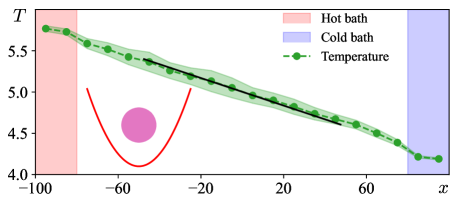
The system consists of $N=2810$ fluid particles and a single Brownian particle. All particles are put into a two-dimensional square box with length $L=200$. The dimensionless density of the fluid is $p_{e}=0.07$, which corresponds to a gas phase. The NVE ensemble is used to carry out the MD simulation. A temperature gradient is established using the Langevin thermostat method [60], by introducing a hot region with temperature $T_{h}=5.8$ near the left boundary, and a cold region with temperature $T_{c}=4.2$ near the right boundary. We choose the reflection boundary condition at $x=\pm 100$, so that there is no macroscopic transport of fluid particles in the steady state. We choose the periodic boundary condition at $y=\pm 100$. See Fig. 1 for an illustration.

We choose the time step of MD integration as $dt=0.001$, and start the simulation from a random state. After running $6\times 10^{5}$ steps, a steady temperature gradient is set up.

To calibrate the simulation, we first simulate an equilibrium fluid by choosing $T_{h}=T_{c}=5$, without inserting the Brownian particle. The radial distribution function (RDF) of fluid particles as a function of $r$ is shown in Fig. 2 (a). The normalized velocity auto-correlation function (VACF) as a function of $t$ is shown in Fig. 2 (b) in log-linear scale. It can be fit well by an exponential:

$$\frac{\langle v(t)v(0)\rangle}{\langle v(0)^{2}\rangle}=e^{-\gamma_{0}t/m_{0}}.$$

(48)

These results indicate the equilibrium nature of the fluid.

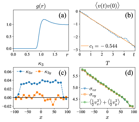
We then introduce the temperature gradient. We cut the system into many slices along the $x$ axis, with thickness $\Delta x=5,{\rm or}\,10$, both of which are longer than the mean free path of fluid particles. Within each slice, the velocity distribution of fluid particles is approximately Gaussian. Deviations from Gaussian may be characterized by the normalized third-order cumulants:

	$\displaystyle\kappa_{3x}$	$\displaystyle=$	$\displaystyle\frac{\langle(v_{x}-\langle v_{x}\rangle)^{3}\rangle}{\langle(v_{x}-\langle v_{x}\rangle)^{2}\rangle^{3/2}},$		(49)
	$\displaystyle\quad\kappa_{3y}$	$\displaystyle=$	$\displaystyle\frac{\langle(v_{y}-\langle v_{y}\rangle)^{3}\rangle}{\langle(v_{y}-\langle v_{y}\rangle)^{2}\rangle^{3/2}}.$		(50)

These cumulants are computed in each slice and shown in Fig. 2 (c). As one can see there, $\kappa_{3y}$ fluctuates around zero, whereas $\kappa_{3x}$ exhibits systematic deviation from zero by a few percent. The latter is evidently related to the heat transport along $x$ direction in the steady state. Hence the pdf of $v_{y}$ is Gaussian, whereas the pdf of $v_{x}$ exhibits a small yet systematic deviation from Gaussian.

We compute the temperature of each slice using three different methods: (1) average kinetic energy $T=\langle\frac{1}{2}v_{x}^{2}\rangle+\langle\frac{1}{2}v_{y}^{2}\rangle$, (2) variance of $v_{x}$, and (3) variance of $v_{y}$. As shown in Fig.2 (d), all three methods are consistent with a constant temperature temperature. The best fit of the temperature profile is

$\displaystyle T(x)=-0.0083\,x+5.005.$

(51)

A Brownian particle is inserted, which also couples to an anisotropic harmonic potential:

$\displaystyle V({\bm{x}})=\frac{1}{2}k_{x}(x-x_{0})^{2}+\frac{1}{2}k_{y}y^{2}.$

(52)

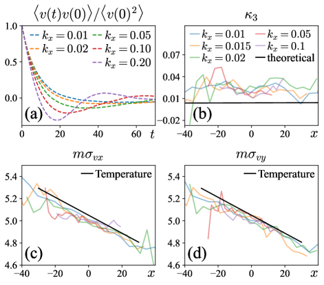
First we set $k_{y}=x_{0}=0$, and compute the VACF of Brownian particle in $x$ direction, for different values of $k_{x}$. As shown in Fig. 3 (a), for $k_{x}>0.05$, the VACF decays in an oscillatory fashion, which means that the system is in the under-damped regime. By contrast for $k_{x}<0.05$, the VACF decays without oscillation, which means that the system is in the over-damped regime. Hence we expect that for $k_{x}<0.05$, the Brownian dynamics is adequately described by the over-damped Langevin equation (2), whereas for $k_{x}>0.05$, the dynamics should be described by under-damped Langevin equation.

Next we compute the velocity pdf of the Brownian particle in each $x$-slice. Similar to the fluid particles, the normalized third order cumulant $\kappa_{3x}$ of the Brownian particle also deviate slightly but systematically from zero, as shown in Fig. 3(b). Furthermore, $\kappa_{3x}$ seems independent of confining potential and of the slice, and is also systematically different from the prediction of Ref. [51].

We also plot the variances of velocity components $v_{x},v_{y}$ of the Brownian particle as a function of $x$. As shown in Fig. 3(c) and (d), the results are consistent with the temperature profile Eq. (51), which is computed using the velocity distributions of the fluid particles. This verifies that the Brownian particle establishes local thermal equilibrium with the fluid within each slice.

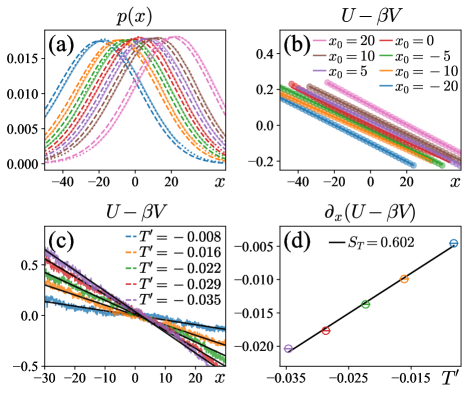
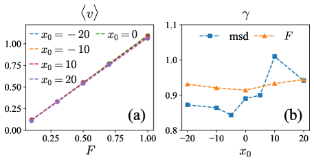
We compute the steady state position pdf of Brownian particle, and use it to obtain the generalized potential via Eq. (1). The results are shown as dotted lines in Fig. 4(a) for different values of $x_{0}$. Also shown there are $e^{-\beta(x)V(x)}$ (dashed lines, normalized properly), which appear always to the left of the steady state pdf. This indicates that the thermophoresis drives Brownian particle to the right (with lower temperature).

We fit the steady state position distribution by $e^{-U_{\rm fit}({\bm{x}};\lambda)}$, where $U_{\rm fit}({\bm{x}};\lambda)$ is given by

$\displaystyle U_{\rm fit}({\bm{x}};\lambda)=\beta({\bm{x}})V({\bm{x}};\lambda)+S_{T}\,{\bm{x}}\cdot\nabla T+b(\lambda),$

(53)

with $T^{\prime}=-0.0083$ as given by Eq. (51), $S_{T}$ is the fitting parameter, whilst $b$ is a normalization constant. As shown by solid lines in Fig. 4(a), the fitting quality is remarkably good.

In Fig. 4(b) we plot $U_{\rm fit}-\beta V$ as a function of $x$, for fixed $k_{x}$ but different values of $x_{0}$. The slope of these straight-lines, which can be understood as the effective thermophoresis force, renormalized by the local temperature $T(x)$, are approximately independent of $x_{0}$. This again verifies the validity of Eq. (53).

Let us now establish the connection between our theory and the thermodynamic theory of thermophoresis [29]. In the latter theory, there is no external potential, the probability current of the Brownian particle is [29]

$${\bm{j}}({\bm{x}})=-D\left(\nabla p({\bm{x}})+S_{T}\,p({\bm{x}})\,\nabla T\right),$$

(54)

where $S_{T}$ is the Soret coefficient, whilst $D$ is the diffusion constant. In general, both $S_{T}$ and $D$ depend on position. However, in the thermodynamic theory of thermophoresis, it is always assumed that the overall variation temperature is small, so that $S_{T}$ and $D$ may be treated as constants.

In our theory, the probability current is given by Eq. (6), where $U$ is given by Eq. (53). In the absence of external potential, Eq. (6) reduces to

$\displaystyle{\bm{j}}({\bm{x}})=-\frac{T({\bm{x}})}{\gamma({\bm{x}})}\left(\nabla p({\bm{x}})+S_{T}\,p({\bm{x}})\,\nabla T\right).$

(55)

This is precisely Eq. (54) with a position-dependent diffusion constant $D({\bm{x}})=T({\bm{x}})/\gamma({\bm{x}})$. Hence the parameter $S_{T}$ in Eq. (53) is precisely the Soret coefficient.

In Fig. 4 (c) we fix $x_{0}=0$, and use simulation data to plot $U-\beta V$ against $x$ for different values of temperature gradient. In Fig. 4 (d) we plot the slope of linear fitting in Fig. 4 (c) against temperature gradient. This clearly demonstrates that the Soret coefficient $S_{T}$ is approximately constant within the region of simulation. Indeed, in the region of simulation, the overall variation of temperature is less than 8%, hence $S_{T}$ can be treated approximately as a constant.

We use two different methods to compute the friction coefficient as a function of $x$. In the first method, we apply a constant force along $y$ direction, and compute the friction coefficient via:

$${\gamma(x_{0})}\langle v_{y}(t)\rangle={F},$$

(56)

where $x_{0}$ is the minimum of the potential Eq. (52). In Fig. 5 (a) the relation between $\langle v_{y}(t)\rangle$ and $F$ is shown for different $x_{0}$, from which we deduce that the dependence of ${\gamma(x_{0})}$ on $x_{0}$ is very weak. The computed friction coefficient is shown as orange symbols in Fig. 5 (b).

In the second method, we set $k_{y}=0$, so that the Brownian particle diffuses freely along $y$ direction, whilst it is confined along $x$ direction. Provided that the Langevin equation (2) is applicable, the mean square displacement (MSD) is given by

$$\langle\Delta y(t)^{2}\rangle=\frac{2T(x_{0})}{\gamma(x_{0})}t,$$

(57)

where $T(x)$ is given by the linear fit Eq. (51). Using Eq. (57) to fit simulation data, we obtain the friction coefficient shown as blue symbols in Fig. 5 (b).

It can be seen from Fig. 5 (b) that whilst two methods are yield generally consistent results, the result of the second method exhibit much larger fluctuations. According to the first method, the friction coefficient is approximately independent of the position along $x$ direction. This is rather expected, since variation of temperature in the simulation region is only a few percent.

We simulate three types of forward processes as well as the corresponding backward processes. In all simulations we fix $k_{y}=0.1$, so that the Brownian particle is localized in $y$ direction. In the first protocol, we fix $k_{x}$ and vary the equilibrium position $x_{0}$ during the process. In the second protocol, we fix $x_{0}$ and vary $k_{x}$. In the third protocol we vary $k_{x},x_{0}$ simultaneously. $x_{0}$, or $k_{x}$, or both, therefore, are the control parameter $\lambda$ we discussed in Sec. II. The details of these protocols are explained in the captions of Fig. 6.

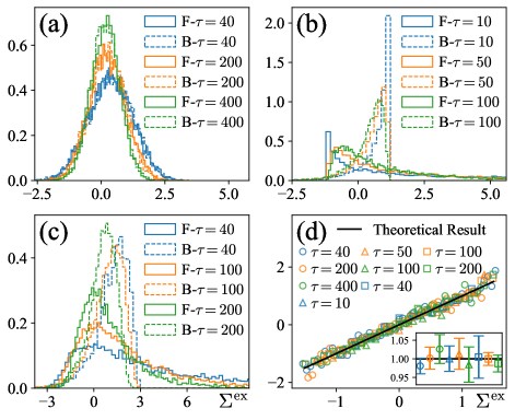
For each process, we sample a large number of trajectories. For each trajectory, we calculate the excess EP using Eq. (40). More specifically, we discretize each trajectory and approximate the excess EP by:

$$\Sigma^{\rm{ex}}[\bm{\gamma}]=\sum_{i}U_{\rm{fit}}(\lambda_{i+1},x_{i})-U_{\rm{fit}}(\lambda_{i},x_{i}),$$

(58)

where $U_{\rm{fit}}$ is given by Eq. (53). The pdfs of $\Sigma^{\rm ex}$ in the forward process are then obtained using histograms. The pdfs of $\Sigma^{\rm ex}$ in the backward process are obtained using similar methods. The results are shown in Fig. 6(a), (b), (c), respectively, for three processes. In Fig. 6(d), the log ratio $\log p_{F}(\Sigma^{\rm ex})/p_{B}(-\Sigma^{\rm ex})$ is plotted against $\Sigma^{\rm ex}$ for all three processes. As shown there, all data collapse to the straight-line with unit slope, as predicted by the excess FT Eq. (43).

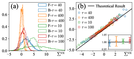
As explained in the captions of Fig. 6 and Fig. 7, in the second and third protocols, the spring constant $k_{x}$ is tuned from $0.01$ to $0.11$. According to the results demonstrated in Fig. 3 (c), for $k_{x}\geq 0.05$, the Brownian dynamics is under-damped, and hence the over-damped Langevin equation (2) is not applicable. Nonetheless, the excess FT seems hold to high precision in these two processes, as can be seen from Fig. 6(d). It then seems that the excess FT Eq. (43) is valid even in the under-damped regime. To test this hypothesis, we also simulate two other protocols where the system is deep in the under-damped regime in the entire process. As shown in Fig. 7, indeed the excess FT (43) remains valid as well.

The validity of the excess FT in the under-damped regime may be understood using the stochastic thermodynamic theory developed in Ref. [21], together with two reasonable assumptions. The Brownian dynamics can be described by certain under-damped Langevin equation. Even though we do not know the concrete form of this equation, we do expect that it obeys local detailed balance. The stochastic thermodynamic theory developed in Ref. [21] is then applicable. (Unlike the over-damped theory as studied in the present work, in the under-damped theory, the house-keeping EP is generically non-vanishing. This point is however irrelevant, since we are only interested in the excess EP. ) The excess EP in the underdamped theory is defined as

$\displaystyle\Sigma^{\rm ex}_{\rm ud}[\bm{\gamma}]=\int_{\bm{\gamma}}d_{\lambda}U_{\rm ud}({\bm{x}},{\bm{p}};\lambda),$

(59)

where ${\bm{p}}$ is the momentum of the Brownian particle and $U_{\rm ud}({\bm{x}},{\bm{p}};\lambda)$ is the generalized potential of the under-damped theory. Here the subscript ud denotes “under-damped”. In fact $\Sigma^{\rm ex}_{\rm ud}[\bm{\gamma}]$ is precisely the functional defined in Eq. (4.62) of Ref. [21]), which is also shown there to obey the fluctuation theorem (c.f. Eq. (4.63) of Ref. [21]):

$\displaystyle\log\frac{p_{F}(\Sigma^{\rm ex}_{\rm ud})}{p_{B}(-\Sigma^{\rm ex}_{\rm ud})}={\Sigma^{\rm ex}_{\rm ud}}.$

(60)

We can decompose the generalized potential $U_{\rm ud}({\bm{x}},{\bm{p}};\lambda)$ into the following form:

$\displaystyle U_{\rm ud}({\bm{x}},{\bm{p}};\lambda)=U_{\bm{X}}({\bm{x}};\lambda)+U_{\bm{P}}({\bm{p}};{\bm{x}},\lambda),$

(61)

such that the conditional steady-state distribution of ${\bm{p}}$ given ${\bm{x}}$ and $\lambda$ is given by

$\displaystyle p^{\rm SS}({\bm{p}}|{\bm{x}},\lambda)=\frac{e^{-U({\bm{x}},{\bm{p}};\lambda)}}{\int e^{-U({\bm{x}},{\bm{p}};\lambda)}d{\bm{p}}}=e^{-U_{\bm{P}}({\bm{p}};{\bm{x}},\lambda)}.$

(62)

It then follows that the marginal steady-state pdf of ${\bm{x}}$ is related to $U_{\bm{X}}$ via

$\displaystyle p^{\rm SS}_{\bm{X}}({\bm{x}})=e^{-U_{\bm{X}}({\bm{x}};\lambda)}.$

(63)

Hence $U_{\bm{X}}({\bm{x}};\lambda)$ is precisely the generalized potential appearing in our over-damped theory.

Now, all results shown in Fig. 3 indicate that the velocity pdfs of the Brownian particle, conditioned on position variable, is independent of the control parameters $\lambda$, i.e. $d_{\lambda}U_{\bm{P}}({\bm{p}};{\bm{x}},\lambda)=0$. From Eq. (61) we then deduce

$\displaystyle d_{\lambda}U_{\rm ud}({\bm{x}},{\bm{p}};\lambda)=d_{\lambda}U_{\bm{X}}({\bm{x}};\lambda),$

(64)

Substituting this back into Eq. (59) we find:

$\displaystyle\Sigma^{\rm ex}_{\rm ud}[\bm{\gamma}]=\int_{\bm{\gamma}}d_{\lambda}U_{\rm ud}=\int_{\bm{\gamma}}d_{\lambda}U_{{\bm{X}}}=\Sigma^{\rm ex}_{\rm od}[\bm{\gamma}].$

(65)

In other words, the excess EP in the under-damped theory is identical to that in the over-damped theory, provided that (i) the under-damped Langevin theory obeys local detailed balance, and (ii) the velocity distribution of the Brownian particle is independent of the control parameter $\lambda$. This explains why the excess FT (43) also holds in the under-damped regime.

References

- [1] Gallavotti, Giovanni, and Ezechiel Godert David Cohen. “Dynamical ensembles in nonequilibrium statistical mechanics.” Physical review letters 74.14 (1995): 2694.
- [2] Jarzynski, C. Equalities and inequalities: Irreversibility and the second law of thermodynamics at the nanoscale. Annu. Rev. Condens. Matter Phys., 2(1), 329-351. (2011)
- [3] Crooks, G. E. Entropy production fluctuation theorem and the nonequilibrium work relation for free energy differences. Physical Review E, 60(3), 2721. (1999)
- [4] Searles, D. J. and Evans, D. J. Fluctuation theorem for stochastic systems. Physical Review E, 60(1), 159 (1999)
- [5] Seifert, U. Stochastic thermodynamics, fluctuation theorems and molecular machines. Reports on progress in physics, 75(12), 126001 (2012).
- [6] Ciliberto, Sergio. Experiments in stochastic thermodynamics: Short history and perspectives. Physical Review X 7.2 (2017): 021051.
- [7] Lebowitz, Joel L., and Herbert Spohn. A Gallavotti-Cohen-type symmetry in the large deviation functional for stochastic dynamics. Journal of Statistical Physics 95 (1999): 333-365.
- [8] Van Zon, R., and Cohen, E. G. D. Stationary and transient work-fluctuation theorems for a dragged Brownian particle. Physical Review E, 67(4), 046102. (2003)
- [9] Peliti, Luca, and Simone Pigolotti. Stochastic Thermodynamics: An Introduction. Princeton University Press, 2021.
- [10] Van den Broeck, Christian. “Stochastic thermodynamics: A brief introduction.” Phys. Complex Colloids 184 (2013): 155-193.
- [11] Hatano, T. and Sasa, S. I. Steady-state thermodynamics of Langevin systems. Physical review letters, 86(16), 3463. (2001)
- [12] Speck, Thomas, and Udo Seifert.“Integral fluctuation theorem for the housekeeping heat.” Journal of Physics A: Mathematical and General 38.34 (2005): L581.
- [13] Chernyak, Vladimir Y., Michael Chertkov, and Christopher Jarzynski. “Path-integral analysis of fluctuation theorems for general Langevin processes.” Journal of Statistical Mechanics: Theory and Experiment 2006.08 P08001 (2006).
- [14] Esposito, M. and Van den Broeck, C. Three detailed fluctuation theorems. Physical review letters, 104(9), 090601. (2010)
- [15] Esposito, M. and Van den Broeck, C. Three faces of the second law. I. Master equation formulation. Physical Review E, 82(1), 011143. (2010)
- [16] Van den Broeck, C. and Esposito, M. Three faces of the second law. II. Fokker-Planck formulation. Physical Review E, 82(1), 011144. (2010)
- [17] Ge, Hao, and Hong Qian. “Physical origins of entropy production, free energy dissipation, and their mathematical representations.” Physical Review E 81.5 (2010): 051133.
- [18] Qian, Hong. “Mesoscopic nonequilibrium thermodynamics of single macromolecules and dynamic entropy-energy compensation.” Physical Review E 65.1 (2001): 016102.
- [19] Qian, Hong. “Entropy production and excess entropy in a nonequilibrium steady-state of single macromolecules.” Physical Review E 65.2 (2002): 021111.
- [20] Glansdorff, Paul, and Ilya Prigogine. Thermodynamic theory of structure, stability and fluctuations. J. Willey & Sons, 1971.
- [21] Mingnan Ding, Fei Liu and Xiangjun Xing. “A Unified Theory for Thermodynamics and Stochastic Thermodynamics of Nonlinear Langevin Systems Driven by Non-conservative Forces” Physical Review Research 4.4 (2022): 043125.
- [22] Sasa, Shin-ichi, and Hal Tasaki. “Steady state thermodynamics.” Journal of statistical physics 125.1 (2006): 125-224.
- [23] Trepagnier, E. H., Jarzynski, C., Ritort, F., Crooks, G. E., Bustamante, C. J. and Liphardt, J. Experimental test of Hatano and Sasa’s nonequilibrium steady-state equality. Proceedings of the National Academy of Sciences, 101(42), 15038-15041.(2004)
- [24] Thalheim, Tobias, et al. “Jarzynski Equality for Soret Equilibria–Virtues of Virtual Potentials.” arXiv preprint arXiv:2009.00950 (2020).
- [25] Ludwig C 1859 Sitz. Ber. Akad. Wiss. Wien 20 539.
- [26] Soret C 1879 Arch. Sci. Phys. Nat. 2 48.
- [27] de Groot S R 1945 L’Effet Soret, Diffusion Thermique Dans Les Phasescondensées (Amsterdam: North-Holland).
- [28] De Groot, Sybren Ruurds, and Peter Mazur. Non-equilibrium thermodynamics. Courier Corporation, 2013.
- [29] Piazza, Roberto, and Alberto Parola. “Thermophoresis in colloidal suspensions.” Journal of Physics: Condensed Matter 20.15 (2008): 153102.
- [30] Piazza, Roberto. “Thermophoresis: moving particles with thermal gradients.” Soft Matter 4.9 (2008): 1740-1744.
- [31] Falasco, Gianmaria, et al. Exact symmetries in the velocity fluctuations of a hot Brownian swimmer. Physical Review E 94.3, 030602. (2016)
- [32] Jerabek-Willemsen, Moran, et al. “MicroScale Thermophoresis: Interaction analysis and beyond.” Journal of Molecular Structure 1077 (2014): 101-113.
- [33] Jerabek-Willemsen, Moran, et al. “Molecular interaction studies using microscale thermophoresis.” Assay and drug development technologies 9.4 (2011): 342-353.
- [34] Thamdrup, Lasse H., Niels B. Larsen, and Anders Kristensen. “Light-induced local heating for thermophoretic manipulation of DNA in polymer micro-and nanochannels.” Nano letters 10.3 (2010): 826-832.
- [35] Baaske, Philipp, et al. “Optical thermophoresis for quantifying the buffer dependence of aptamer binding.” Angewandte Chemie International Edition 49.12 (2010): 2238-2241.
- [36] Wen, Y., Liu, Q. and Liu, Y. “Temperature gradient-driven motion and assembly of two-dimensional (2D) materials on the liquid surface: a theoretical framework and molecular dynamics simulation. ” Physical Chemistry Chemical Physics, 22(41), 24097-24108.(2020)
- [37] Becton, M. and Wang, X. Thermal gradients on graphene to drive nanoflake motion. Journal of chemical theory and computation, 10(2), 722-730. (2014)
- [38] Dehbi, A. A stochastic Langevin model of turbulent particle dispersion in the presence of thermophoresis. International Journal of Multiphase Flow, 35(3), 219-226.(2009)
- [39] Pakravan, H. A. and Yaghoubi, M. Combined thermophoresis, Brownian motion and Dufour effects on natural convection of nanofluids. International Journal of Thermal Sciences, 50(3), 394-402.(2011)
- [40] Helden, L., Eichhorn, R. and Bechinger, C. Direct measurement of thermophoretic forces. Soft matter, 11(12), 2379-2386. (2015)
- [41] Braibanti, M., Vigolo, D. and Piazza, R. Does thermophoretic mobility depend on particle size? Physical review letters, 100(10), 108303.(2008)
- [42] Rurali, R. and Hernandez, E. R. Thermally induced directed motion of fullerene clusters encapsulated in carbon nanotubes. Chemical Physics Letters, 497(1-3), 62-65. (2010)
- [43] Schoen, P. A., Walther, J. H., Poulikakos, D. and Koumoutsakos, P. Phonon assisted thermophoretic motion of gold nanoparticles inside carbon nanotubes. Applied Physics Letters, 90(25), 253116. (2007)
- [44] Duhr, S. and Braun, D. Thermophoretic depletion follows Boltzmann distribution. Physical review letters, 96(16), 168301. (2006)
- [45] Duhr, S. and Braun, D. Why molecules move along a temperature gradient. Proceedings of the National Academy of Sciences, 103(52), 19678-19682. (2006)
- [46] Kroy, Klaus, Dipanjan Chakraborty, and Frank Cichos. “Hot microswimmers.” The European Physical Journal Special Topics 225 (2016): 2207-2225.
- [47] Würger, A. . Hydrodynamic boundary effects on thermophoresis of confined colloids. Physical review letters, 116(13), 138302. (2016)
- [48] Würger, Alois. Thermal non-equilibrium transport in colloids. Reports on Progress in Physics 73(12), 126601. (2010)
- [49] Burelbach, Jérôme, et al. A unified description of colloidal thermophoresis. The European Physical Journal E 41, 1-12. (2018).
- [50] Falasco, Gianmaria, and Klaus Kroy. Nonisothermal fluctuating hydrodynamics and Brownian motion. Physical Review E 93.3, 032150. (2016)
- [51] Celani, A., Bo, S., Eichhorn, R. and Aurell, E. Anomalous thermodynamics at the microscale. Physical review letters, 109(26), 260603. (2012)
- [52] Marino, Raffaele, Ralf Eichhorn, and Erik Aurell. “Entropy production of a Brownian ellipsoid in the over-damped limit.” Physical Review E 93.1 (2016): 012132.
- [53] Sancho, J. M. Brownian colloids in underdamped and overdamped regimes with nonhomogeneous temperature. Physical Review E, 92(6), 062110. (2015)
- [54] Polettini, M. Diffusion in nonuniform temperature and its geometric analog. Physical Review E, 87(3), 032126. (2013)
- [55] Ding, M., Tu, Z. and Xing, X. Covariant formulation of nonlinear Langevin theory with multiplicative Gaussian white noises. Physical Review Research, 2(3), 033381. (2020).
- [56] Gardiner, Crispin W. Handbook of Stochastic Methods, 3rd ed., Berlin: Springer, 2004.
- [57] Ding, M. and Xing, X. (2022). Covariant nonequilibrium thermodynamics from Ito-Langevin dynamics. Physical Review Research, 4(3), 033247.
- [58] Ding, M., Tu, Z. and Xing, X. Strong coupling thermodynamics and stochastic thermodynamics from the unifying perspective of time-scale separation. Physical Review Research, 4(1), 013015. (2022).
- [59] Plimpton, S. Fast parallel algorithms for short-range molecular dynamics. Journal of computational physics, 117(1), 1-19. (1995).
- [60] Schneider, T. and Stoll, E. Molecular-dynamics study of a three-dimensional one-component model for distortive phase transitions. Physical Review B, 17(3), 1302. (1978)
- [61] Fodor, É., Nardini, C., Cates, M. E., Tailleur, J., Visco, P., & Van Wijland, F., How far from equilibrium is active matter? Physical review letters 117. 3 , 038103. (2016)
- [62] Mandal, Dibyendu, Katherine Klymko, and Michael R. DeWeese. Entropy production and fluctuation theorems for active matter. Physical review letters 119.25, 258001. (2017)
- [63] U. Seifert. Entropy production along a stochastic trajectory and an integral fluctuation theorem. Phys. Rev. Lett., 95(4):040602, 2005.