Stochastic noise can be helpful for variational quantum algorithms

Junyu Liu Pritzker School of Molecular Engineering, The University of Chicago, Chicago, IL 60637, USA Chicago Quantum Exchange, Chicago, IL 60637, USA Kadanoff Center for Theoretical Physics, The University of Chicago, Chicago, IL 60637, USA qBraid Co., Chicago, IL 60615, USA Frederik Wilde Dahlem Center for Complex Quantum Systems, Freie Universität Berlin, Berlin, 14195, Germany Antonio Anna Mele Dahlem Center for Complex Quantum Systems, Freie Universität Berlin, Berlin, 14195, Germany Liang Jiang Pritzker School of Molecular Engineering, The University of Chicago, Chicago, IL 60637, USA Chicago Quantum Exchange, Chicago, IL 60637, USA Jens Eisert Dahlem Center for Complex Quantum Systems, Freie Universität Berlin, Berlin, 14195, Germany Helmholtz-Zentrum Berlin für Materialien und Energie, 14109 Berlin, Germany Fraunhofer Heinrich Hertz Institute, 10587 Berlin, Germany

Saddle points constitute a crucial challenge for first-order gradient descent algorithms. In notions of classical machine learning, they are avoided for example by means of stochastic gradient descent methods. In this work, we provide evidence that the saddle points problem can be naturally avoided in variational quantum algorithms by exploiting the presence of stochasticity. We prove convergence guarantees and present practical examples in numerical simulations and on quantum hardware. We argue that the natural stochasticity of variational algorithms can be beneficial for avoiding strict saddle points, i.e., those saddle points with at least one negative Hessian eigenvalue. This insight that some levels of shot noise could help is expected to add a new perspective to notions of near-term variational quantum algorithms.

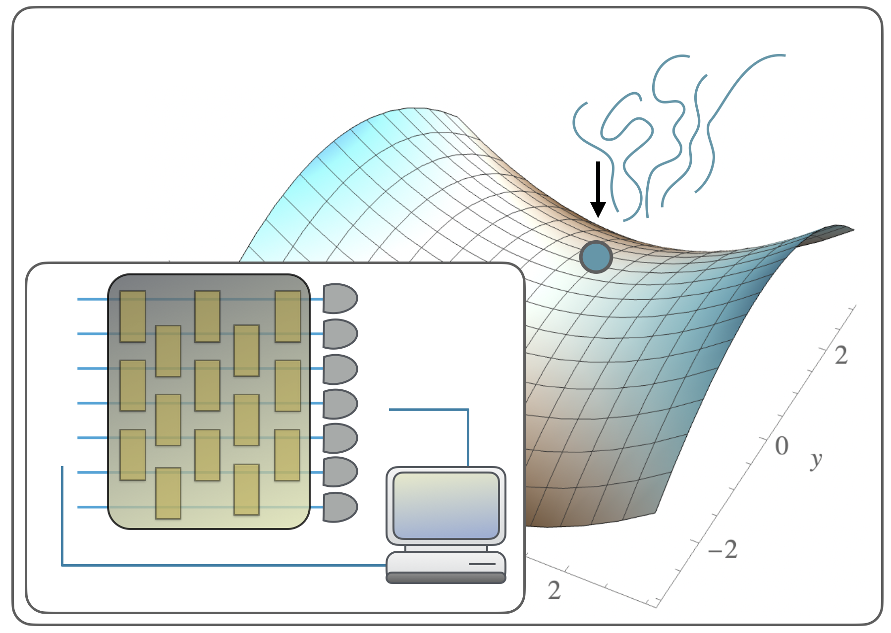
Quantum computing has for many years been a hugely inspiring theoretical idea. Already in the 1980ies it was suggested that quantum devices could possibly have superior computational capabilities over computers operating based on classical laws Feynman-1986 ; QuantumTuring . It is a relatively recent development that devices have been devised that may indeed have computational capabilities beyond classical means GoogleSupremacy ; Boixo ; SupremacyReview ; jurcevic_demonstration_2021 . These devices are going substantially beyond what was possible not long ago. And still, they are unavoidably noisy and imperfect for many years to come. The quantum devices that are available today and presumably will be in the near future are often conceived as hybrid quantum devices running variational quantum algorithms Cerezo_2021 , where a quantum circuit is addressed by a substantially larger surrounding classical circuit. This classical circuit takes measurements from the quantum device and appropriately varies variational parameters of the quantum device in an update. Large classes of variational quantum eigensolvers (VQE), the quantum approximate optimization algorithm (QAOA) and models for quantum-assisted machine learning are thought to operate along those lines, based on suitable loss functions to be minimized Peruzzo ; Kandala ; McClean_2016 ; QAOA ; Lukin ; bharti_2021_noisy ; VariationalReview . In fact, many near-term quantum algorithms in the era of noisy intermediate-scale quantum (NISQ) computing preskill_quantum_2018 belong to the class of variational quantum algorithms. While this is an exciting development, it puts a lot of burden to understanding how reasonable and practical classical control can be conceived.

Generally, when the optimization space is high-dimensional updates of the variational parameters are done via gradient evaluations PhysRevA.99.032331 ; bergholm2018pennylane ; pennylane ; Gradients , while zeroth-order and second-order methods are, in principle, also applicable, but typically only up to a limited number of parameters. This makes a lot of sense, as one may think that going downhill in a variational quantum algorithms is a good idea. That said, the concomitant classical optimization problems are generally not convex optimization problems and the variational landscapes are marred by globally suboptimal local optima and saddle points. In fact, it is known that the problems of optimizing variational parameters of quantum circuits are computationally hard in worst case complexity Bittel . While this is not of too much concern in practical considerations (since it is often sufficient to find a “good” local minimum instead of the global minimum) and resembles an analogous situation in classical machine learning, it does point to the fact that one should expect a rugged optimization landscape, featuring different local minima as well as saddle points. Such saddle points can indeed be a burden to feasible and practical classical optimization of variational quantum algorithms.

Refer to caption — Figure 1: Stochasticity in variational quantum algorithms can help in avoiding (strict) saddle points.

In this work, we establish the notion that in such situations, small noise levels can actually be of substantial help. More precisely, we show that some levels of statistical noise (specifically the kind of noise that naturally arises from a finite number of measurements to estimate quantum expectation values) can even be beneficial. We get inspiration from and build on a powerful mathematical theory in classical machine learning: there, theorems have been established that say that “noise” can help gradient-descent optimization not to get stuck at saddle points JordanSaddlePoints ; jain2017non . Building on such ideas we show that they can be adapted and developed to be applicable to the variational quantum algorithms setting. Then we argue that the “natural” statistical noise of a quantum experiment can play the role of the artificial noise that is inserted by hand in classical machine learning algorithms to avoid saddle points. We maintain the precise and rigorous mindset of Ref. JordanSaddlePoints , but show that the findings have practical importance and can be made concrete use of when running variational quantum algorithms on near-term quantum devices. In previous studies it has been observed anecdotally that small levels of noise can indeed be helpful for improving the optimization procedure duffield_bayesian_2022 ; Gradients ; Jansen ; Rosenkranz ; Lorenz ; Yelin2 ; gu_adaptive_2021 . What is more, variational algorithms have been seen as being noise-robust in a sense PhysRevA.102.052414 . That said, while in the past rigorous convergence guarantees have been formulated for convex loss functions of VQAs Gradients ; gu_adaptive_2021 , in this work we focus on the non-convex scenario, where saddle points and local minima are present. Such a systematic and rigorous analysis of the type we have conducted that explains the origin of the phenomenon of noise facilitating optimization has been lacking.

It is important to stress that for noise we refer to in our theorems is the type of noise that adds stochasticity to the gradient estimations, such as the use of a finite number of measurements or the zero-average fluctuations that are involved in real experiments. Also, instances of global depolarizing noise are covered as discussed in Appendix .2. Thus, in this case, noise does not mean the generic quantum noise that results from the interaction with the environment characterized by completely positive and trace-preserving (CPTP) maps, which can be substantially detrimental to the performance of the algorithm DePalmaVQAs ; Stilck_Fran_a_2021 . In addition, it has been shown that noisy CPTP maps in the circuit may significantly worsen the problem of barren plateaus NoisyBP_Wang_2021 ; McClean_2018 which is one of the main obstacles to the scalability of variational quantum algorithms (VQAs).

We perform numerical experiments, and we show examples where optimizations with gradient descent without noise get stuck at saddle points, whereas if we add some noise, we can escape this problem and get to the minimum—convincingly demonstrating the functioning of the approach. We verify the latter not only in a numerical simulation, but also making use of data of a real IBM quantum machine.

Preliminaries

In our work, we will show how a class of saddle points, the so-called strict saddle points, can be avoided in noisy gradient descent. In developing our machinery, we build strongly on the rigorous results laid out in Ref. JordanSaddlePoints and uplift them to the quantum setting at hand. For this, we do method development in its own right. First, we introduce some useful definitions and theorems (see Ref. JordanSaddlePoints for a more in-depth discussion).

Throughout this work, we consider the problem of minimizing a function $\mathcal{L}:\mathbb{R}^{p}\to\mathbb{R}$ . We indicate its gradient at $\theta$ as $\partial\mathcal{L}(\theta)$ and its Hessian matrix at point $\theta$ as $\partial^{2}\mathcal{L}(\theta)$ . We denote as $\left\|\cdot\right\|_{2}$ the $l_{2}$ norm of a vector. $\left\|\cdot\right\|_{HS}$ and $\left\|\cdot\right\|_{\infty}$ denote respectively the Hilbert-Schmidt norm and the largest eigenvalue norm of a matrix. We denote as $\lambda_{\min}(\cdot)$ the minimum eigenvalue of a matrix.

Definition 1 ( $L$ -Lipschitz function).

A function $g:\mathbb{R}^{p}\to\mathbb{R}^{d}$ is $L$ -Lipschitz if and only if

\displaystyle\left\|g(\theta)-g(\phi)\right\|_{2}\leq L\left\|\theta-\phi\right\|_{2}

(1)

for every $\theta$ and $\phi$ .

Definition 2 ( $\beta$ -strong smoothness).

A differentiable function $\mathcal{L}:\mathbb{R}^{p}\to\mathbb{R}$ is called $\beta$ -strongly smooth if and only if its gradient is a $\beta$ -Lipschitz function, i.e.,

\displaystyle\left\|\partial\mathcal{L}(\theta)-\partial\mathcal{L}(\phi)\right\|_{2}\leq\beta\left\|\theta-\phi\right\|_{2}\leavevmode\nobreak\ ,

(2)

for every $\theta$ and $\phi$ .

Definition 3 (Stationary point).

If $\mathcal{L}$ is differentiable, ${\theta^{*}}$ is defined a stationary point if

\left\|\partial\mathcal{L}({\theta^{*}})\right\|_{2}=0.

(3)

Definition 4 ( $\epsilon$ -approximate stationary point).

If $\mathcal{L}$ is differentiable, ${\theta^{*}}$ is defined an $\epsilon$ -approximate stationary point if

\left\|\partial\mathcal{L}({\theta^{*}})\right\|_{2}\leq\epsilon.

(4)

Definition 5 (Local minimum, local maximum, and saddle point).

If $\mathcal{L}$ is differentiable, a stationary point ${\theta^{*}}$ is a

•

local minimum, if there exists $\delta>0$ such that $\mathcal{L}({\theta^{*}})\leq\mathcal{L}(\theta)$ for any $\theta$ with $\left\|\theta-{\theta^{*}}\right\|_{2}\leq\delta$ .
•

Local maximum, if there exists $\delta>0$ such that $\mathcal{L}({\theta^{*}})\geq\mathcal{L}(\theta)$ for any $\theta$ with $\left\|\theta-{\theta^{*}}\right\|_{2}\leq\delta$ .
•

Saddle point, otherwise.

Definition 6 ( $\rho$ -Lipschitz Hessian).

A twice differentiable function $\mathcal{L}$ has $\rho$ -Lipschitz Hessian matrix $\partial^{2}\mathcal{L}$ if and only if

\displaystyle\left\|\partial^{2}\mathcal{L}(\theta)-\partial^{2}\mathcal{L}(\phi)\right\|_{\operatorname{HS}}\leq\rho\left\|\theta-\phi\right\|_{2}

(5)

for every $\theta$ and $\phi$ (where $\left\|\cdot\right\|_{\operatorname{HS}}$ is the Hilbert-Schmidt norm).

Definition 7 (Gradient descent).

Given a differentiable function $\mathcal{L}$ , the gradient descent algorithm is defined by the update rule

\displaystyle\theta_{i}^{t+1}=\theta_{i}^{t}-\eta{{\partial}_{i}}\mathcal{L}(\theta^{t}){{\color[rgb]{0,0,0}\definecolor[named]{pgfstrokecolor}{rgb}{0,0,0}\pgfsys@color@gray@stroke{0}\pgfsys@color@gray@fill{0},}}

(6)

where $\eta>0$ is called learning rate.

The convergence time of the gradient descent algorithm is given by the following theorem JordanSaddlePoints .

Theorem 8 (Gradient descent complexity).

Given a $\beta$ -strongly smooth function $\mathcal{L}(\cdot)$ , for any $\epsilon>0$ , if we set the learning rate as $\eta=1/\beta$ , then the number of iterations required by the gradient descent algorithm such that it will visit an $\epsilon$ -approximate stationary point is

\mathcal{O}\left({\frac{\beta\left(\mathcal{L}\left(\mathbf{\theta}_{0}\right)-\mathcal{L}^{\star}\right)}{\epsilon^{2}}}\right),

where $\mathbf{\theta}_{0}$ is the initial point and $\mathcal{L}^{\star}$ is the value of $\mathcal{L}$ computed in the global minimum.

It is important to note that this result does not depend on the number of free parameters. Also, the stationary point at which the algorithm will converge is not necessarily a local minimum, but can also be a saddle point. Note that a generic saddle point satisfies $\lambda_{\min}(\partial^{2}\mathcal{L}(\theta_{s}))\leq 0$ where $\lambda_{\min}(\cdot)$ is the minimum eigenvalue. Now we define a subclass of saddle points.

Definition 9 (Strict saddle point).

$\theta_{s}$ is a strict saddle point for a twice differentiable function $\mathcal{L}$ if and only if $\theta_{s}$ is a stationary point and if the minimum eigenvalue of the Hessian is $\lambda_{\min}(\partial^{2}\mathcal{L}(\theta_{s}))<0$ .

Adding the strict condition, we remove the case in which a saddle point satisfies $\lambda_{\min}(\partial^{2}\mathcal{L}(\theta_{s}))=0$ . Moreover, note that a local maximum respects our definition of strict saddle point. Analogously to Ref. JordanSaddlePoints , in this work, we focus on avoiding strict saddle points. Hence, it is useful to introduce the following definition.

Definition 10 (Second-order stationary point).

Given a twice differentiable function $\mathcal{L}(\cdot),\mathbf{\theta^{*}}$ is a second-order stationary point if and only if

\partial\mathcal{L}(\mathbf{\theta^{*}})=\mathbf{0},\quad\text{ and }\quad\lambda_{\min}(\partial^{2}\mathcal{L}(\mathbf{\theta^{*}}))\geq 0.

(7)

Definition 11 ( $\epsilon$ -second-order stationary point).

For a $\rho$ -Hessian Lipschitz function $\mathcal{L}(\cdot),\mathbf{\theta^{*}}$ is an $\epsilon$ -second-order stationary point if

|\partial\mathcal{L}(\mathbf{\theta^{*}})|_{2}\leq\epsilon\quad\text{ and }\quad\lambda_{\min}(\partial^{2}\mathcal{L}(\mathbf{\theta^{*}}))\geq-\sqrt{\rho\epsilon}.

(8)

Gradient descent makes a non-zero step only when the gradient is non-zero, and thus in the non-convex setting it will be stuck at saddle points. A simple variant of GD is the perturbed gradient descent (PGD) method JordanSaddlePoints which adds randomness to the iterates at each step.

Definition 12 (Perturbed gradient descent).

Given a differentiable function $\mathcal{L}:\mathbb{R}^{p}\to\mathbb{R}$ , the perturbed gradient descent algorithm is defined by the update rule

\displaystyle\theta_{i}^{t+1}=\theta_{i}^{t}-\eta\left({{\partial}_{i}}\mathcal{L}\left({{\theta}^{t}}\right)+{{\zeta}^{t}}\right)\leavevmode\nobreak\ {{\color[rgb]{0,0,0}\definecolor[named]{pgfstrokecolor}{rgb}{0,0,0}\pgfsys@color@gray@stroke{0}\pgfsys@color@gray@fill{0},}}

(9)

where $\eta>0$ is the learning rate and ${{\zeta}^{t}}$ is a normally distributed random variable with mean $\mu=0$ and variance $\sigma^{2}={r^{2}}/{p}$ with $r\in\mathbb{R}$ .

In Ref. JordanSaddlePoints , the authors show that if we pick $r=\tilde{\Theta}(\epsilon)$ , PGD will find an $\epsilon$ -second-order stationary point in a number of iterations that has only a poly-logarithmic dependence on the number of free parameters, i.e., it has the same complexity of (standard) gradient descent up to poly-logarithmic dependence.

Theorem 13 (JordanSaddlePoints ).

Let the function $\mathcal{L}:\mathbb{R}^{d}\to\mathbb{R}$ be $\beta$ strongly smooth and such that it has a $\rho$ Lipschitz-Hessian. Then, for any $\epsilon,\delta>0$ , the $PGD$ algorithm starting at the point $\theta_{0}$ , with parameters $\eta=\tilde{\Theta}(1/\beta)$ and $r=\tilde{\Theta}(\epsilon)$ , will visit an $\epsilon-$ second-order stationary point at least once in the following number of iterations, with probability at least $1-\delta$

\tilde{\mathcal{O}}\left(\frac{\beta\left(\mathcal{L}\left(\theta_{0}\right)-\mathcal{L}^{\star}\right)}{\epsilon^{2}}\right)

where $\tilde{\mathcal{O}}$ and $\tilde{\Theta}$ hide poly-logarithmic factors in $p,\beta,\rho,1/\epsilon,1/\delta$ and $\Delta_{\mathcal{L}}:=\mathcal{L}\left(\theta_{0}\right)-\mathcal{L}^{\star}$ . $\mathbf{\theta}_{0}$ is the initial point and $\mathcal{L}^{\star}$ is the value of $\mathcal{L}$ computed in the global minimum.

This theorem has been proven in Ref. JordanSaddlePoints for Gaussian distributions, but the authors have pointed out that this is not strictly necessary and that it can be generalized to other types of probability distributions in which appropriate concentration inequalities can be applied (for a more in-depth discussion, see Ref. JordanSaddlePoints ).

In Ref. ExpTimeSaddle , it has been shown that although the standard GD (without perturbations) almost always escapes the saddle points asymptotically Lee2017 , there are (non-pathological) cases in which the optimization requires exponential time to escape. This highlights the importance of using gradient descent with perturbations.

Statistical noise in variational quantum algorithms

Our analysis focuses on variational quantum algorithms in which the loss function to be minimized has the following form

\displaystyle\mathcal{L}\left(\theta\right):=\bra{0}U^{\dagger}(\theta)OU(\theta)\ket{0}

(10)

where $O$ is a Hermitian operator and $U(\theta)$ is a parameterized unitary of the form

\displaystyle U({\theta}):=\prod_{\ell=1}^{p}W_{\ell}\exp\left(i\theta_{\ell}X_{\ell}\right).

(11)

where $W_{\ell}$ and $X_{\ell}$ are respectively fixed unitaries and Hermitian operators. Theorem 13 above assumes that the loss function to minimize is $\beta$ -strongly smooth and has a $\rho$ -Lipschitz Hessian. To guarantee that these conditions are met for loss functions of parametrized quantum circuits, we provide the following theorem.

Theorem 14.

The loss function given in equation (10) with $\theta$ being a $p$ -dimensional vector is $\beta$ -strongly smooth and has a $\rho$ -Lipschitz Hessian. In particular, we have

		$\displaystyle\beta\leq 2^{2}p\\|O\\|_{\infty}\max_{j=1,\dots,p}\\|X_{j}\\|_{\infty}^{2},$		(12)
		$\displaystyle\rho\leq 2^{3}p^{\frac{3}{2}}\\|O\\|_{\infty}\max_{j=1,\dots,p}\\|X_{j}\\|_{\infty}^{3}.$		(13)

We provide a detailed proof in Appendix .1. It is important to observe that for typical VQAs, the observable $O$ associated to the loss function and the components $X_{i}$ have an operator norm that grows at most polynomially with the number of qubits, so also $\beta$ and $\rho$ will grow at most polynomially. This is because the circuit depth $p$ must be chosen to be at most $\mathcal{O}\left({\rm poly}(n)\right)$ , $X_{l}$ as well as $O$ are usually chosen to be Pauli strings in which case their operator norms is $1$ or to be linear combinations of $\mathcal{O}\left({\rm poly}(n)\right)$ many Pauli strings with $\mathcal{O}\left({\rm poly}(n)\right)$ coefficients (as in QAOA), therefore by the triangle inequality their operator norm is bounded by $\mathcal{O}\left({\rm poly}(n)\right)$ . Sometimes $O$ is also chosen to be a quantum state Cerezo_2021 , therefore with operator norm bounded by $1$ . Hence, the number of iterations in Theorem 13 does not grow exponentially in the number of qubits.

The previous results can be easily generalized for the case of differentiable and bounded loss functions which are functions of expectation values, i.e.,

\displaystyle\mathcal{L}(\theta)=f\left(\left\langle 0\left|{{U}^{\dagger}}(\theta)OU(\theta)\right|0\right\rangle\right).

(14)

In fact, we observe that if $\mathcal{L}$ and $g$ are Lipschitz functions, then

	$\displaystyle\|\mathcal{L}(g({\theta}))-\mathcal{L}(g({\theta^{\prime}}))\|$	$\displaystyle\leq L_{\mathcal{L}}\\|g(\theta)-g(\theta^{\prime})\\|_{2}$
		$\displaystyle\leq L_{\mathcal{L}}L_{g}\\|\theta-\theta^{\prime}\\|_{2}.$

In addition, if $\mathcal{L}$ is a differentiable function with bounded derivatives on a convex set, then (because of the mean value theorem) $\mathcal{L}$ is Lipschitz on this set. From this follows that if $\mathcal{L}$ is a differentiable function with bounded derivatives of a quantum expectation value (whose image defines a bounded $\mathbb{R}$ interval), then it is Lipschitz. Moreover the sum of Lipschitz functions is a Lipschitz function. Therefore, functions of expectation values commonly used in machine learning tasks, such as the mean squared error, satisfy the Lipschitz condition.

Moreover, Theorem 13 assumes that at each step of the gradient descent a normally distributed random variable is added to the gradient, namely $\theta_{i}^{t+1}=\theta_{i}^{t}-\eta\left({{\partial}_{i}}\mathcal{L}\left({{\theta}^{t}}\right)+{{\zeta}^{t}}\right)$ . In VQAs the partial derivatives are commonly estimated using a finite number of measurements, such as by the so-called parameter shift rule GradientsQcomp . Here, the update rule for the gradient descent is

\theta_{i}^{t+1}=\theta_{i}^{t}-\eta\hat{g}_{i}\left({{\theta}^{t}}\right),

(16)

where $\hat{g}_{i}\left({{\theta}^{t}}\right)$ is an estimator of the partial derivative ${{\partial}_{i}}\mathcal{L}\left({{\theta}^{t}}\right)$ obtained by a finite number of measurements $N_{\rm shots}$ from the quantum device. Moreover, we define

\hat{\zeta}^{t}_{N_{\rm shots}}:={{\partial}_{i}}\mathcal{L}\left({{\theta}^{t}}\right)-\hat{g}_{i}\left({{\theta}^{t}}\right).

(17)

Note that $\hat{\zeta}^{t}_{N_{\rm shots}}$ is a random variable with zero expectation value. Therefore, we have

\theta_{i}^{t+1}=\theta_{i}^{t}-\eta\left({{\partial}_{i}}\mathcal{L}\left({{\theta}^{t}}\right)+\hat{\zeta}^{t}_{N_{\rm shots}}\right){{\color[rgb]{0,0,0}\definecolor[named]{pgfstrokecolor}{rgb}{0,0,0}\pgfsys@color@gray@stroke{0}\pgfsys@color@gray@fill{0}.}}

(18)

The “noise” $\hat{\zeta}^{t}_{N_{\rm shots}}$ will play the role of the noise that is added by hand in the perturbed-gradient descent algorithm 12. However, we cannot control exactly the distribution of such random variable, nor the variance. However, it is to be expected that in the limit of many measurement shots, by the central limit theorem, the noise encountered in practice will be close to the noise considered here, a Gaussian distribution.

Numerical and quantum experiments

In this section, we discuss the results of numerical and quantum experiments we have performed to show that stochasticity can help escape saddle points. Our results suggest that statistical noise leads to a non-vanishing probability of not getting stuck in a saddle point and thereby reaching a lower value of the loss function. These numerical experiments also complement the rigorous results that are proven to be valid under very precisely defined conditions, while the intuition developed here is expected to be more broadly applicable, so that the rigorous results can be seen as proxies for a more general mindset. Modify (16) We have also observed this phenomena in a real IBM quantum device. We have done so to convincingly stress the significance of our results in practice.

Let us first consider the Hamiltonian ${{\color[rgb]{0,0,0}\definecolor[named]{pgfstrokecolor}{rgb}{0,0,0}\pgfsys@color@gray@stroke{0}\pgfsys@color@gray@fill{0}O}}=\sum_{i=1}^{N=4}Z_{i}$ . The loss function we consider is defined as the expectation value of such a Hamiltonian over the parametrized quantum circuit qml.StronglyEntanglingLayers implemented in Pennylane bergholm2018pennylane , where two layers of the circuit are used. In all our experiments we first initialize the parameters in multiple randomly chosen values. Next, we select the initial points for which the optimization process gets stuck at a suboptimal loss-function value, thereby focusing on cases in which saddle points constitute a significant problem for the (noiseless) optimizer. This selection can be justified by the fact that the loss function defined by $O$ is trivial to begin with. The relevant aspect of this experiment is to study situations in which optimizer encounters saddle points. As such we exclusively investigate these specifically selected initial points by subsequently initializing the noisy optimizer with them.

As a proof of principle, we first show the results of an exact simulation (i.e., the expectation values are not estimated using a finite number of shots, but are calculated exactly) in which noise is added manually at each step of the gradient descent. The probability distribution associated to the noise is chosen to be a Gaussian distribution with mean $\mu=0$ and variance $\sigma^{2}=r^{2}$ . Figure 2 shows the difference between the noiseless, and noisy calculations with the same initial conditions of the gradient descent, when the noise is from random Gaussian perturbations added manually. Figure 3 shows the performance of the experiment, defined as ${1}/({\mathcal{L}-\mathcal{L}_{\text{opt}}})$ as a function of the noise parameter. Here, we can find a critical value of noise, leading to saddle-point avoidance. Figure 4 specifically addresses quantum noise levels, with simulated results about purely statistical noise levels (shot noise) and device noise (simulated by making use of the noise model of actual quantum hardware IBM Qiskit).

It should be noted that including device noise generally also means dealing with completely positive trace preserving maps that can lead to a different loss function, with new local minima, new saddle points and a flatter landscape NoisyBP_Wang_2021 . However, even in this case we observe an improvement in performance using the same initial parameters leading to the saddle point in the noiseless case. This is perfectly in line with the intuition developed here, as long as the effective noise emerging can be seen as a small perturbation of the reference circuit featuring a given loss landscape that is then in effect perturbed by stochastic noise.

Aside from the quantum machine learning example, we also provide another instance in variational quantum eigensolvers (VQEs). Here, we use the Hamiltonian associated to the Hydrogen molecule $\text{H}_{2}$ , which is a 4-qubit Hamiltonian obtained by the fermionic one performing a Jordan-Wigner transformation. We specifically use the same circuit from h2.xyz, the Hydrogen VQE example in Pennylane pennylane . Also here, given initial parameters that led to saddle points in the noiseless case, we find that starting by the same parameters and adding noise can lead to saddle-point avoidance. Results are shown in Fig. 5 where we compare the noiseless and noisy simulation.

To further provide evidence of the functioning of our approach suggested and the rigorous insights established, we put the findings into contact of the results of a real experiment example in the IBM Qiskit environment. We use the Hamiltonian ${{\color[rgb]{0,0,0}\definecolor[named]{pgfstrokecolor}{rgb}{0,0,0}\pgfsys@color@gray@stroke{0}\pgfsys@color@gray@fill{0}O}}=\sum_{i=1}^{N=4}Z_{i}$ that we used in our first numerical simulation with four qubits and two layers. We run the experiment using as initial condition the one that lead to a saddle point in the noiseless case. We use the IBMQ_Jakarta device with 10000 shots. The result in Figure 6 shows that it is possible to obtain a lower value of the cost function than that of the simulation without noise that has been stuck in a saddle point.

Conclusion and outlook

In this work, we have proposed small stochastic noise levels as an instrument to facilitate variational quantum algorithms. This noise can be substantial, but should not be too large: The way a noise level can strike the balance in overcoming getting stuck in saddle points and being detrimental is in some ways reminiscent of the phenomenon of stochastic resonance in statistical physics StochasticResonance . This is a phenomenon in which suitable small increases in levels of noise can increase in a metric of the quality of signal transmission, resonance or detection performance, rather than a decrease. Here, also fine tuned noise levels can facilitate resonance behavior and avoid getting trapped.

On a higher level, our work invites to think more deeply about the use of classical stochasic noise in variational quantum algorithms as well as ways to prove performance guarantees about such approaches. For example, Metropolis sampling inspired classical algorithms in which a stochastic process satisfying detailed balance is set up over variational quantum circuits may assist in avoiding getting stuck in rugged energy landscapes.

It is also interesting to note that the technical results obtained here provide further insights into an alternative interpretation of the setting discussed here. Instead of regarding the noise as stochastic noise that facilitates the optimization in the proven fashion established here, one may argue that the noise channels associated with the noise alter the variational landscapes in the first place PhysRevA.104.022403 ; PRXQuantum.2.040309 . For example, such quantum channels are known to be able to break parameter symmetries in over-parameterized variational algorithms. It is plausible to assume that these altered variational landscapes may be easier to optimize over. It is an interesting observation in its own right that the technical results obtained here also have implications to this alternative viewpoint, as the convergence guarantees are independent on the interpretation.

It is the hope that the present work puts the role of stochasticity in variational quantum computing into a new perspective, and contributes to a line of thought exploring the use of suitable noise and sampling for enhancing quantum computing schemes.

Author contributions

J. E. and J. L. have suggested to exploit classical stochastic noise in variational quantum algorithms, and to prove convergence guarantees for the performance of the resulting algorithms. J. L., A. A. M., F. W., and J. E. have proven the theorems of convergence. J. L. and F. W. have devised and conducted the numerical simulations. J. L. has performed quantum device experiments under the guidance of L. J. All authors have discussed the results and have written the manuscript.

Acknowledgments

J. L. is supported in part by International Business Machines (IBM) Quantum through the Chicago Quantum Exchange, and the Pritzker School of Molecular Engineering at the University of Chicago through AFOSR MURI (FA9550-21-1-0209). F. W., A. A. M. and J. E. thank the BMBF (Hybrid, MuniQC-Atoms, DAQC), the BMWK (EniQmA, PlanQK), the MATH+ Cluster of Excellence, the Einstein Foundation (Einstein Unit on Quantum Devices), the QuantERA (HQCC), the Munich Quantum Valley (K8), and the DFG (CRC 183) for support. LJ acknowledges support from the ARO (W911NF-18-1-0020, W911NF-18-1-0212), ARO MURI (W911NF-16-1-0349), AFOSR MURI (FA9550-19-1-0399, FA9550-21-1-0209), DoE Q-NEXT, NSF (EFMA-1640959, OMA-1936118, EEC-1941583), NTT Research, and the Packard Foundation (2013-39273). This research used resources of the Oak Ridge Leadership Computing Facility, which is a DOE Office of Science User Facility supported under Contract DE-AC05-00OR22725.

References

(1) Feynman, R. P. Quantum mechanical computers. Found. Phys. 16, 507–531 (1986).
(2) Deutsch, D. Quantum theory, the Church-Turing principle and the universal quantum computer. Proc. Roy. Soc. A 400, 97–117 (1985).
(3) Arute, F. et al. Quantum supremacy using a programmable superconducting processor. Nature 574, 505–510 (2019).
(4) Boixo, S. et al. Characterizing quantum supremacy in near-term devices. Nature Phys. 14, 595–600 (2018).
(5) Hangleiter, D. & Eisert, J. Computational advantage of quantum random sampling. arXiv:2206.04079 (2022).
(6) Jurcevic, P. et al. Demonstration of quantum volume 64 on a superconducting quantum computing system. Quantum Sci. Technol. 6, 025020 (2021).
(7) Cerezo, M. et al. Variational quantum algorithms. Nature Rev. Phys. 3, 625–644 (2021).
(8) Peruzzo, A. et al. A variational eigenvalue solver on a photonic quantum processor. Nature Comm. 5, 4213 (2014).
(9) Kandala, A. et al. Hardware-efficient variational quantum eigensolver for small molecules and quantum magnets. Nature 549, 242 (2017).
(10) McClean, J. R., Romero, J., Babbush, R. & Aspuru-Guzik, A. The theory of variational hybrid quantum-classical algorithms. New J. Phys. 18, 023023 (2016).
(11) Farhi, E., Goldstone, J. & Gutmann, S. A quantum approximate optimization algorithm. arxiv:1411.4028 (2014).
(12) Zhou, L., Wang, S.-T., Choi, S., Pichler, H. & Lukin, M. Quantum approximate optimization algorithm: Performance, mechanism, and implementation on near-term devices. Phys. Rev. X 10, 021067 (2020).
(13) Bharti, K. et al. Noisy intermediate-scale quantum (NISQ) algorithms. Rev. Mod. Phys. 94, 015004 (2022).
(14) Tilly, J. et al. The variational quantum eigensolver: a review of methods and best practices. arXiv:2111.05176 (2021).
(15) Preskill, J. Quantum computing in the NISQ era and beyond. arXiv:1801.00862 (2018).
(16) Schuld, M., Bergholm, V., Gogolin, C., Izaac, J. & Killoran, N. Evaluating analytic gradients on quantum hardware. Phys. Rev. A 99, 032331 (2019).
(17) Bergholm, V., Izaac, J., Schuld, M., Gogolin, C. & Killoran, N. Pennylane: Automatic differentiation of hybrid quantum-classical computations. arXiv:1811.04968 (2018).
(18) https://pennylane.ai/qml/demos/tutorial_vqe_qng.html#stokes2019.
(19) Sweke, R. et al. Stochastic gradient descent for hybrid quantum-classical optimization. Quantum 4, 314 (2020).
(20) Bittel, L. & Kliesch, M. Training variational quantum algorithms is NP-hard. Phys. Rev. Lett. 127, 120502 (2021).
(21) Jin, C., Netrapalli, P., Ge, R., Kakade, S. M. & Jordan, M. I. On nonconvex optimization for machine learning: Gradients, stochasticity, and saddle points. arXiv:1902.04811 (2019).
(22) Jain, P. & Kar, P. Non-convex optimization for machine learning. arXiv:1712.07897 (2017).
(23) Duffield, S., Benedetti, M. & Rosenkranz, M. Bayesian learning of parameterised quantum circuits (2022). ArXiv:2206.07559 [quant-ph, stat].
(24) Borras, K. et al. Impact of quantum noise on the training of quantum generative adversarial networks. arXiv:2203.01007 (2022).
(25) Duffield, S., Benedetti, M. & Rosenkranz, M. Bayesian learning of parameterised quantum circuits. arXiv:2206.07559 (2022).
(26) Oliv, M., Matic, A., Messerer, T. & Lorenz, J. M. Evaluating the impact of noise on the performance of the variational quantum eigensolver. arXiv:2209.12803 .
(27) Patti, T. L., Najafi, K., Gao, X. & Yelin, S. F. Entanglement devised barren plateau mitigation. arXiv:2012.12658 (2020).
(28) Gu, A., Lowe, A., Dub, P. A., Coles, P. J. & Arrasmith, A. Adaptive shot allocation for fast convergence in variational quantum algorithms. arXiv.2108.10434 (2021).
(29) Gentini, L., Cuccoli, A., Pirandola, S., Verrucchi, P. & Banchi, L. Noise-resilient variational hybrid quantum-classical optimization. Phys. Rev. A 102, 052414 (2020).
(30) De Palma, G., Marvian, M., Rouzé, C. & França, D. S. Limitations of variational quantum algorithms: a quantum optimal transport approach. arXiv:2204.03455 (2022).
(31) França, D. S. & García-Patrón, R. Limitations of optimization algorithms on noisy quantum devices. Nature Phys. 17, 1221–1227 (2021).
(32) Wang, S. et al. Noise-induced barren plateaus in variational quantum algorithms. Nature Comm. 12, 6961 (2021).
(33) McClean, J. R., Boixo, S., Smelyanskiy, V. N., Babbush, R. & Neven, H. Barren plateaus in quantum neural network training landscapes. Nature Comm. 9 (2018).
(34) Du, S. S. et al. Gradient descent can take exponential time to escape saddle points. arXiv:1705.10412 (2017).
(35) Lee, J. D. et al. First-order methods almost always avoid saddle points. arXiv:1710.07406 (2017).
(36) Schuld, M., Bergholm, V., Gogolin, C., Izaac, J. & Killoran, N. Evaluating analytic gradients on quantum hardware. Phys. Rev. A 99, 032331 (2019).
(37) Benzi, R., Sutera, A. & Vulpiani, A. The mechanism of stochastic resonance. J. Phys. A 14, L453–L457 (1981).
(38) Fontana, E., Fitzpatrick, N., Ramo, D. M. n., Duncan, R. & Rungger, I. Evaluating the noise resilience of variational quantum algorithms. Phys. Rev. A 104, 022403 (2021).
(39) Haug, T., Bharti, K. & Kim, M. Capacity and quantum geometry of parametrized quantum circuits. PRX Quantum 2, 040309 (2021).
(40) Patel, D., Coles, P. J. & Wilde, M. M. Variational quantum algorithms for semidefinite programming. arXiv:2112.08859 (2021).
(41) Pólya, G. Über eine Aufgabe der Wahrscheinlichkeitsrechnung betreffend die Irrfahrt im Straßennetz. Math. Ann. 84, 149–160 (1921).
(42) Montroll, E. W. Random walks in multidimensional spaces, especially on periodic lattices. J. Soc. Ind. Appl. Math. 4, 241–260 (1956).
(43) Liu, J., Tacchino, F., Glick, J. R., Jiang, L. & Mezzacapo, A. Representation learning via quantum neural tangent kernels. arXiv:2111.04225 (2021).
(44) Liu, J. et al. An analytic theory for the dynamics of wide quantum neural networks. arXiv:2203.16711 (2022).
(45) Liu, J., Lin, Z. & Jiang, L. Laziness, barren plateau, and noise in machine learning. arXiv:2206.09313 (2022).

Supplementary material

.1 Strong smoothness and Lipschitz-Hessian property

In this section we provide a proof of Theorem 14. As stated in the main text we focus our analysis on ansatz circuits of the form

U({\theta}):=\prod_{\ell=1}^{p}W_{\ell}\exp\left(i\theta_{\ell}X_{\ell}\right)

(19)

where $W_{\ell}$ and $X_{\ell}$ are respectively fixed unitaries and Hermitian operators. As a reminder, we want to show that the loss function

\mathcal{L}({\theta})=\left\langle 0\left|{{U}^{\dagger}}({\theta})OU({\theta})\right|0\right\rangle

(20)

is $\beta$ -strongly smooth and has a $\rho$ -Lipschitz Hessian, with

	$\displaystyle\beta$	$\displaystyle\leq 2^{2}p\left\\|O\right\\|_{\infty}\max_{j=1,\dots,p}\left\\|X_{j}\right\\|_{\infty}^{2},$		(21)
	$\displaystyle\rho$	$\displaystyle\leq 2^{3}p^{\frac{3}{2}}\left\\|O\right\\|_{\infty}\max_{j=1,\dots,p}\left\\|X_{j}\right\\|_{\infty}^{3}.$		(22)

To begin, we state three important facts about Lipschitz constants of multi-variate functions.

Lemma 15.

If $\mathcal{L}:\mathbb{R}^{p}\to\mathbb{R}$ is differentiable with bounded partial derivatives, then

L=\sqrt{p}\max_{j}\left(\sup_{{\theta}}\left|\frac{\partial\mathcal{L}({\theta})}{\partial\theta_{j}}\right|\right)

(23)

is the Lipschitz constant for $\mathcal{L}$ .

The proof is given in Ref. WildeSDP (Lemma 7).

Lemma 16.

If $\mathcal{L}:\mathbb{R}^{p}\to\mathbb{R}^{M}$ is a function with all its $M$ components Lipschitz functions with Lipschitz constant $L_{i}$ , then $\mathcal{L}$ has Lipschitz constant $L=\sqrt{\sum_{i=1}^{M}L_{i}^{2}}$ .

The proof is given in Ref. WildeSDP (Lemma 8). Equipped with these facts we can proceed to derive an upper bound for the Lipschitz constant of functions from $\mathbb{R}^{p}$ to $\mathbb{R}^{M}$ .

Lemma 17.

If $g:\mathbb{R}^{p}\to\mathbb{R}^{M}$ is a differentiable function with bounded gradient, then its Lipschitz constant $L$ satisfies

L\leq\sqrt{pM}\max_{i,j}\left(\sup_{{\theta}}\left|\frac{\partial g_{i}({\theta})}{\partial\theta_{j}}\right|\right),

(24)

where $g_{i}({\theta})$ the $i$ -th component of $\theta\mapsto g({\theta})$ .

Proof.

Using Lemma 15 and 16, we have

	$\displaystyle L=\sqrt{\sum_{i=1}^{M}L_{i}^{2}}$	$\displaystyle\leq\sqrt{M}\max_{i}(L_{i})$
		$\displaystyle=\sqrt{pM}\max_{i,j}\left(\sup_{{\theta}}\left\|\frac{\partial g_{i}({\theta})}{\partial\theta_{j}}\right\|\right),$		(25)

where $L_{i}$ is the Lipschitz constant of the $i$ -th component of $\mathcal{L}$ as defined in Lemma 16. ∎

Next, we focus on loss functions of the type in equation (10).

Lemma 18.

The loss function as defined in Eq. (20) (with ${\theta}\in\mathbb{R}^{p}$ ) satisfies

\displaystyle\max_{i_{1},i_{2}\dots i_{k}}\left(\sup_{{\theta}}\left|\frac{\partial^{k}\mathcal{L}({\theta})}{\partial\theta_{i_{k}}\cdots\partial\theta_{i_{2}}\partial\theta_{i_{1}}}\right|\right)\leq 2^{k}\left\|O\right\|_{\infty}\max_{j=1,\dots,p}\left\|X_{j}\right\|_{\infty}^{k}

(26)

where $U(\theta)$ is given by Eq. (19).

Proof.

We introduce the standard multi-index notation. For this, we have

\displaystyle\partial^{\alpha}\mathcal{L}({\theta}):=\frac{\partial^{k}\mathcal{L}({\theta})}{\partial\theta_{i_{k}}\cdots\partial\theta_{i_{2}}\partial\theta_{i_{1}}}.

(27)

With this, the multi derivative of the loss reads

	$\displaystyle\partial^{\alpha}\mathcal{L}({\theta})$	$\displaystyle=\bra{0}\partial^{\alpha}\left({U}^{\dagger}({\theta})OU({\theta})\right)\ket{0}$
		$\displaystyle=\sum_{\beta:\beta\leq\alpha}\left(\begin{array}[]{l}\alpha\\ \beta\end{array}\right)\bra{0}\left(\partial^{\beta}{U}^{\dagger}({\theta})\right)O\left(\partial^{\alpha-\beta}U({\theta})\right)\ket{0},$		(30)

where we have expolited the generalized Leibniz formula

\displaystyle\partial^{\alpha}(fg)=\sum_{\beta:\beta\leq\alpha}\left(\begin{array}[]{l}\alpha\\ \beta\end{array}\right)\left(\partial^{\beta}f\right)\partial^{\alpha-\beta}g.

(33)

We have

$\displaystyle\|\partial^{\alpha}\mathcal{L}\|$	$\displaystyle\leq\sum_{\beta:\beta\leq\alpha}\left(\begin{array}[]{l}\alpha\\ \beta\end{array}\right)\left\|\bra{0}\left(\partial^{\beta}{U}^{\dagger}({\theta})\right)O\left(\partial^{\alpha-\beta}U({\theta})\right)\ket{0}\right\|$	(35)
	$\displaystyle=2^{\|\alpha\|}\max_{\gamma:\gamma\leq\alpha}\left\|\bra{0}\left(\partial^{\gamma}{U}^{\dagger}({\theta})\right)O\,\partial^{\alpha-\gamma}U({\theta})\ket{0}\right\|$
	$\displaystyle\leq 2^{\|\alpha\|}\max_{\gamma:\gamma\leq\alpha}\left\\|\left(\partial^{\gamma}{U}^{\dagger}({\theta})\right)O\,\partial^{\alpha-\gamma}U({\theta})\right\\|_{\infty}$
	$\displaystyle\leq 2^{\|\alpha\|}\max_{\gamma:\gamma\leq\alpha}\left\\|\partial^{\gamma}{U}^{\dagger}({\theta})\right\\|_{\infty}\\|O\\|_{\infty}\left\\|\partial^{\alpha-\gamma}U({\theta})\right\\|_{\infty},$	(36)

where we have used the triangle inequality and the multi-binomial theorem formula to write

\sum_{\beta:\beta\leq\alpha}\left(\begin{array}[]{l}\alpha\\ \beta\end{array}\right)=2^{|\alpha|},

(37)

the fact that

\left|\bra{0}A\ket{0}\right|\leq\left\|A\ket{0}\right\|_{2}\leq\left\|A\right\|_{\infty},

(38)

which follows immediately by Cauchy-Schwarz and the sub-additivity of the $\|\cdot\|_{\infty}$ norm. Using the form of the parameterized unitary in Eq. (19), we can also observe that

$\displaystyle\\|\partial^{\gamma}{U}^{\dagger}({\theta})\\|_{\infty}$	$\displaystyle=\left\\|\frac{\partial^{\gamma_{p}}}{\partial\theta^{\gamma_{p}}_{p}}\cdots\frac{\partial^{\gamma_{1}}}{\partial\theta^{\gamma_{1}}_{1}}{U}^{\dagger}({\theta})\right\\|_{\infty}$
	$\displaystyle\leq\\|X_{1}\\|^{\gamma_{1}}_{\infty}\cdots\\|X_{p}\\|^{\gamma_{p}}_{\infty}$
	$\displaystyle\leq\left(\max_{j=1,\dots,p}\\|X_{j}\\|_{\infty}\right)^{\gamma_{1}+\cdots+\gamma_{p}}$
	$\displaystyle\leq\max_{j=1,\dots,p}\\|X_{j}\\|^{\left\|\gamma\right\|}$	(39)

where we have used that the subadditivity of the infinity norm and the fact that the spectral norm of a unitary matrix is given by the unity. Similarly, we have

\|\partial^{\alpha-\gamma}{U}({\theta})\|_{\infty}\leq\max_{j=1,\dots,p}\|X_{j}\|^{|\alpha|-|\gamma|}.

(40)

Therefore, combining the previous two inequalities with Eq. (36), we have

	$\displaystyle\|\partial^{\alpha}\mathcal{L}\|$	$\displaystyle\leq 2^{\|\alpha\|}\\|O\\|_{\infty}\max_{j=1,\dots,p}\\|X_{j}\\|^{\|\alpha\|}$
		$\displaystyle=2^{k}\\|O\\|_{\infty}\max_{j=1,\dots,p}\\|X_{j}\\|^{k},$		(41)

where we have used $\left|\alpha\right|=k$ . ∎

We are now ready to provide the proof of Theorem 14. Since the loss function is a combination of sin and cosin functions, its derivatives exist and are bounded, and from this it follows that the loss function is strongly smooth and its Hessian is Lipschitz. However, it is worth explicitly calculating $\beta$ and $\rho$ and bounding them to verify, for example, the scaling with the number of qubits.

Proof.

We have the $\beta$ -smooth constant defined by the smallest $\beta$ with

\displaystyle\left\|\partial\mathcal{L}({\theta})-\partial\mathcal{L}({\theta^{\prime}})\right\|\leq\beta\left\|{\theta}-{\theta^{\prime}}\right\|,

(42)

which means we need to consider the Lipschitz constant for the $p$ -dimensional function $\partial\mathcal{L}({\theta})$ . Using Lemma 17 where $g({\theta})=\partial\mathcal{L}$ and $M=p$ , we have

\beta\leq p\max_{i,j}\left(\sup_{{\theta}}\left|\frac{\partial^{2}\mathcal{L}({\theta})}{\partial\theta_{i}\partial\theta_{j}}\right|\right).

(43)

Applying Lemma 18, we find

\beta\leq 2^{2}p\|O\|_{\infty}\max_{i}(\|X_{i}\|_{\infty})^{2},

(44)

where we have used the matrix spectral (operator) norm.

The $\rho$ -Hessian constant is defined as

\displaystyle\|\partial^{2}\mathcal{L}({\theta})-\partial^{2}\mathcal{L}({\theta^{\prime}})\|_{\operatorname{H.S.}}\leq\rho\|\theta-\theta^{\prime}\|_{2}

(45)

where $\partial^{2}\mathcal{L}$ is the Hessian matrix and we have used the Hilbert-Schmidt matrix norm. Note that the Hilbert Schmidt norm of a matrix is the 2-norm of the matrix vectorization $\operatorname{vec}(\cdot)$ . We can now apply Lemma 17, where $M=p^{2}$ since the Hessian is a map from $\mathbb{R}^{p}$ to $\mathbb{R}^{p\times p}$ . Defining $g({\theta})=\operatorname{vec}\left(\partial^{2}\mathcal{L}({\theta})\right)$ we find

\rho\leq p^{\frac{3}{2}}\max_{i,j,k}\left(\sup_{{\theta}}\left|\frac{\partial^{3}\mathcal{L}({\theta})}{\partial\theta_{k}\partial\theta_{i}\partial\theta_{j}}\right|\right).

(46)

Thus, applying Lemma 18, we arrive at

\rho\leq 2^{3}p^{\frac{3}{2}}\|O\|_{\infty}\max_{i}(\|X_{i}\|_{\infty})^{3}.

(47)

∎

.2 Discussion on more general noise

In this section, we discuss the impact of more general noise. We assume that we have device noise that is constant in time, i.e., for each state preparation, effectively, we always encounter the same CPTP maps acting on the initial state. This will change the state $\rho(\theta)$ at the end of the circuit to a noisy instance $\rho_{\text{noisy}}(\theta)$ which can be modeled as the applications of parametrized unitary layers interspersed with suitable CPTP maps to the initial state $\rho_{0}$ :

\displaystyle{{\color[rgb]{0,0,0}\definecolor[named]{pgfstrokecolor}{rgb}{0,0,0}\pgfsys@color@gray@stroke{0}\pgfsys@color@gray@fill{0}\rho_{\text{noisy}}(\theta)=\mathcal{N}_{p}\circ\mathcal{U}_{p}\circ\cdots\circ\mathcal{N}_{1}\circ\mathcal{U}_{1}\left(\rho_{0}\right)}}

(48)

where $\mathcal{N}_{i}$ and $\mathcal{U}_{i}$ are respectively noisy CPTP maps and the parametrized unitary channels. As a result, the loss function changes to:

\displaystyle\mathcal{L}_{\text{noisy}}(\theta)=\Tr(H\rho_{\text{noisy}}(\theta)),

(49)

i.e., we now have to optimize an inherently different loss function. Still, to estimate the noisy loss function $\mathcal{L}_{\text{noisy}}$ , also here we will have to deal with statistical noise derived by the finite number of measurements. In particular for the case of global depolarizing noise with depolarizing noise parameter $q\in\left[0,1\right]$

\displaystyle\mathcal{N}_{i}\left(\cdot\right)=\left(1-q\right)\left(\cdot\right)+q\Tr\left(\cdot\right)\frac{\mathbb{1}}{2^{n}}

(50)

the cost function will be

\displaystyle\mathcal{L}_{\text{noisy}}(\theta)=\left(1-q\right)^{p}\mathcal{L}\left(\theta\right)+\left(1-\left(1-q\right)^{p}\right)\frac{\Tr\left(H\right)}{2^{n}}

(51)

Therefore, in such case, the landscape of the cost function will be rescaled and shifted, but will preserve features of the noiseless-landscape like the position of saddle points.

Proof.

By Eq. (48), we have

	$\displaystyle\rho_{\text{noisy}}(\theta)=$	$\displaystyle\left(1-q\right)\mathcal{N}_{p}\circ\mathcal{U}_{p}\circ\cdots\circ\mathcal{N}_{2}\circ\mathcal{U}_{2}\left(\mathcal{U}_{1}\left(\rho_{0}\right)\right)$
		$\displaystyle+q\,\frac{\mathbb{1}}{2^{n}}$
	$\displaystyle=$	$\displaystyle\left(1-q\right)^{2}\mathcal{N}_{p}\circ\mathcal{U}_{p}\circ\cdots\circ\mathcal{N}_{3}\circ\mathcal{U}_{3}\left(\mathcal{U}_{2}\circ\mathcal{U}_{1}\left(\rho_{0}\right)\right)$
		$\displaystyle+q\left(\left(1-q\right)+1\right)\left(\frac{\mathbb{1}}{2^{n}}\right)$
	$\displaystyle=$	$\displaystyle\left(1-q\right)^{p}\rho\left(\theta\right)+q\left(\sum^{p-1}_{k=0}(1-q)^{k}\right)\frac{\mathbb{1}}{2^{n}}$
	$\displaystyle=$	$\displaystyle\left(1-q\right)^{p}\rho\left(\theta\right)+q\frac{1-\left(1-q\right)^{p}}{q}\frac{\mathbb{1}}{2^{n}}.$

Plugging such a state into the definition of the noisy cost function (49), we have the result. ∎

.3 Additional numerical results

In this section, we show additional numerical results to the one reported in the main text. In Fig. 8, we show the estimated probability of avoiding the saddle point as a function of the number of shots, for the loss function given by the expectation value of the local Pauli Hamiltonian ${H}=\sum_{i=1}^{N=4}Z_{i}$ over the circuit qml.StronglyEntanglingLayers (see Fig. 7) in Pennylane bergholm2018pennylane where two layers have been used.

One could directly extend our results towards the description of situations involving more qubits. Here, we consider eight qubits and two layers of quantum gates. Now the loss landscape is richer and we can converge at more integers. For instance, we find convergence at $-3$ , $-4$ , $-5$ , $-6$ for different initial conditions. Figure 10 illustrates saddle-point avoidance with different noise levels when noise is selected from Gaussian distributions. Figure 9 illustrates the performances among different sizes of noise levels and one can again find a critical value of the noise which leads to the saddle-point avoidance.

In Fig. 11, we depict the performances as a function of the noise level obtained for the $\text{H}_{2}$ molecule experiment.

Furthermore, we try to find the relation between the convergence time $T$ and the noise size $r\sim\epsilon$ . With the same setup, we plot the dependence between the convergence time (the time where we approximately get the true minimum) and the size of the noise in the Gaussian distribution case, in Fig. 12. We find that the convergence time indeed decays when we add more noise, and we fit the scaling and find where $T\sim\#/\epsilon^{0.6}$ , which is consistent with the bound $T\sim\#/\epsilon^{2}$ in theory. In Section .4, we provide a heuristic derivation on the scaling $T\sim 1/\epsilon^{2}$ by dimensional analysis and other analytic heuristics.

Finally, we examine the generality of initial points that could be trapped by saddle points. In Fig. 13, we have studied 1000 initial variational angles randomly sampled between $[0,2\pi]$ in the same setup of Fig. 3 with four qubits. Under identical gradient descent conditions, we have observed that 305 initial points lead to saddle points rather than local minima in the absence of noise. Consequently, the estimated probability of getting stuck near saddle points in our study is approximately $30.5\%$ . Classical machine learning theory demonstrates that saddle points are not anomalies but rather common features in loss function landscapes, making stochastic gradient descents crucial for most traditional machine learning applications. We anticipate that in quantum machine learning, getting trapped by saddle points will also be a common occurrence, with the likelihood of entrapment increasing in higher-dimensional settings. Here’s a straightforward explanation: Saddle points are determined by the signs of Hessian eigenvalues. In models with $p$ parameters, there are p Hessian eigenvalues. Assuming equal chances of positive and negative eigenvalues, the probability of obtaining a positive semi-definite Hessian becomes exponentially small ( $2^{-p}$ ). Therefore, as the model size increases, saddle points become increasingly prevalent.

.4 Analytic heuristics

In this section, we provide a set of analytic heuristics about predicting the noisy convergence and the critical noise with significant improvements in performance. Our derivation is physical and heuristic, but we expect that they will be helpful to understand the nature of the noisy dynamics during gradient descent in the quantum devices. The results developed corroborate the idea that a balance between too little and too much noise will have to be struck.

.4.1 Brownian motion and the Polya’s constant

One of the simplest heuristics about noisy gradient descent is the theory of Brownian motion. Define $p(d)$ , also known as Polya’s constant, as the likelihood that a random walk on a $d$ -dimensional lattice has the capability to return to its starting point. It has been proven that polya1921aufgabe ,

\displaystyle p(1)=p(2)=1\leavevmode\nobreak\ ,

(52)

but

\displaystyle p(d\geq 3)<1\leavevmode\nobreak\ .

(53)

In fact, $d\mapsto p(d)$ has the closed formula montroll1956random

\displaystyle p(d)=1-{{\left(\int_{0}^{\infty}{{{\left[{{I}_{0}}\left(\frac{t}{d}\right)\right]}^{d}}}{{e}^{-t}}dt\right)}^{-1}}\leavevmode\nobreak\ ,

(54)

where $d>3$ is the number of training parameter in our case, and $I$ is the modified Bessel function of the first kind. One could compute numerical values of the probability $p(d)$ for increasing $d$ . From $d=4$ to $d=8$ , it changes monotonically from 0.19 to 0.07. It is hard to compute the integral accurately because of damping, but it is clear that it is decaying and will vanish for large $d$ . In our problem, we could regard the process of noisy gradient descent as random walks in the space of variational angles. One could regard the returning probability roughly as the probability of coming back to the saddle point from the minimum. Thus, the statement about lattice random walk gives us intuition that it is less likely to return back when we have a large number of variational angles.

.4.2 Guessing $1/\epsilon^{2}$ by dimensional analysis

One of the primary progress of the technical result presented in Ref. ExpTimeSaddle is the $1/\epsilon^{2}$ dependence on the convergence time $T$ with the size of the noise $\epsilon>0$ . Here, we show that one could guess such a result in the small $\eta$ limit (where $\eta$ is the learning rate) simply by dimensional analysis. Starting from the definition of the gradient descent algorithm,

\displaystyle\delta{\theta_{i}}={\theta_{i}}(t+1)-{\theta_{i}}(t)=-\eta\frac{{\partial\mathcal{L}}}{{\partial{\theta_{i}}}}\leavevmode\nobreak\ ,

(55)

we can instead study the variation of the loss function

	$\displaystyle\delta\mathcal{L}=\mathcal{L}(t+1)-\mathcal{L}(t)\approx\sum\limits_{i}{\frac{{\partial\mathcal{L}}}{{\partial{\theta_{i}}}}\delta{\theta_{i}}}=-\eta\sum\limits_{i}{\frac{{\partial\mathcal{L}}}{{\partial{\theta_{i}}}}\frac{{\partial\mathcal{L}}}{{\partial{\theta_{i}}}}}$
	$\displaystyle=-4\eta\sum\limits_{i}{\frac{{\partial\sqrt{\mathcal{L}}}}{{\partial{\theta_{i}}}}\frac{{\partial\sqrt{\mathcal{L}}}}{{\partial{\theta_{i}}}}}\mathcal{L}\leavevmode\nobreak\ .$		(56)

Here, we use the assumption where $\eta$ is small, such that we could expand the loss function change $\delta\mathcal{L}$ by the first order Taylor expansion. Now we define

\displaystyle{K_{\mathcal{L}}}:=4\sum\limits_{i}{\frac{{\partial\sqrt{\mathcal{L}}}}{{\partial{\theta_{i}}}}\frac{{\partial\sqrt{\mathcal{L}}}}{{\partial{\theta_{i}}}}}\leavevmode\nobreak\ ,

(57)

and we have

\displaystyle\delta\mathcal{L}=-\eta{K_{\mathcal{L}}}\mathcal{L}\leavevmode\nobreak\ .

(58)

If $K_{\mathcal{L}}$ is a constant (and we could assume it is true since we are doing dimensional analysis), we get

\displaystyle\mathcal{L}(t)={(1-\eta{K_{\mathcal{L}}})^{t}}\approx{e^{-\eta{K_{\mathcal{L}}}t}}\leavevmode\nobreak\ .

(59)

In general, we can assume a time-dependent solution as

\displaystyle\mathcal{L}(t)={(1-\eta{K_{\mathcal{L}}(t)})^{t}}\approx{e^{-\eta{K_{\mathcal{L}}(t)}t}}\leavevmode\nobreak\ .

(60)

Now let us think about how the scaling of convergence time will be with noise. First, in the $\eta\to 0$ limit, for small $\eta$ the convergence time would get smaller, not larger (since it is immediately dominated by noise). So it is not possible that $T\sim 1/\eta$ to some powers in $\eta$ . So the only possibility is

\displaystyle T=\mathcal{O}(1)+\mathcal{O}(\eta)+\mathcal{O}({\eta^{2}})\ldots\leavevmode\nobreak\

(61)

in the scaling of $\eta$ . We will thus focus on the first $\mathcal{O}(1)$ term in the small $\eta$ limit. Furthermore, from the form $e^{-\eta{K_{\mathcal{L}}}t}$ we know that $T\sim 1/K_{\mathcal{L}}$ .

Now let us count the dimension, assuming $\theta_{i}$ has the $\theta$ -dimension 1 and $L$ has the $\theta$ -dimension 0. From the gradient descent formula, $\eta$ has the $\theta$ -dimension 2, $K_{\mathcal{L}}$ has the $\theta$ -dimension -2, and $\epsilon$ has the $\theta$ -dimension 1. The time $T$ is dimensionless since $\eta{K_{\mathcal{L}}}T$ is dimensionless and appears in the exponent. Thus, since we know that $T\sim 1/K_{\mathcal{L}}$ , there must be an extra factor balancing the $\theta$ -dimension of $K_{\mathcal{L}}$ . The only choice is $\epsilon^{2}$ , and we cannot use $\eta$ because we are studying the term with the $\eta$ -scaling $\mathcal{O}(1)$ . Thus, we immediately get, $T\sim{1}/{(K_{\mathcal{L}}\epsilon^{2})}$ . That is how we get the dependence $T\sim 1/\epsilon^{2}$ by dimensional analysis. Note that the estimation only works in the small $\eta$ limit. More generally, we have

\displaystyle T=\sum\limits_{m,n>2m}{\mathcal{O}\left(\frac{{{\eta}^{n-2m}}}{K_{\mathcal{L}}^{m}{{\epsilon}^{n}}}\right)}\leavevmode\nobreak\

(62)

if we assume that the expression of $T$ is analytic.

.4.3 Large-width limit

The dependence $T\sim 1/\epsilon^{2}$ can also be made plausible using the quantum neural tangent kernel (QNTK) theory. The QNTK theory has been established Liu:2021wqr ; Liu:2022eqa ; Liu:2022rhw in the limit where we have a large number of trainable angles $d$ and a small learning rate $\eta$ , with the quadratic loss function. According to Ref. Liu:2022rhw , we use the loss function

\displaystyle\mathcal{L}(\theta)=\frac{1}{2}\left(\left\langle\Psi_{0}\left|U^{\dagger}(\theta)OU(\theta)\right|\Psi_{0}\right\rangle-O_{0}\right)^{2}=:\frac{1}{2}\varepsilon^{2}\leavevmode\nobreak\ .

(63)

Here, we make predictions on the eigenvalue of the operator $O$ towards $O_{0}$ . And we use $U(\theta)$ as the variational ansatz. The gradient descent algorithm is

\displaystyle{{\theta}_{i}}(t+1)-{{\theta}_{i}}(t)=:\delta{{\theta}_{i}}=-\eta\frac{\partial{\mathcal{L}}}{\partial{{\theta}_{i}}}\leavevmode\nobreak\

(64)

when there is no noise. Furthermore, we hereby model the noise by adding Gaussian random variables in each step of the update. Those random fluctuations are independently distributed through $\Delta\theta_{i}\sim\mathcal{N}(0,\epsilon^{2})$ . Now, in the limit where $d$ is large, we have an analytic solution of the convergence time, given by

\displaystyle T\approx\frac{\log\left(\frac{\epsilon}{\sqrt{2{{\varepsilon}^{2}}(0)\eta-{{\varepsilon}^{2}}(0){{\eta}^{2}}K+{{\epsilon}^{2}}}}\right)}{\log(1-\eta K)}\leavevmode\nobreak\ ,

(65)

where $K:=K_{\mathcal{L}}/2$ . In the small $\eta$ limit, we have

\displaystyle T\approx\frac{{{\varepsilon}^{2}}(0)}{\epsilon^{2}K}\leavevmode\nobreak\ .

(66)

This gives substance to the claim in the dimensional analysis.

.4.4 Critical noise from random walks

Moreover, using the result from Ref. Liu:2022rhw , we can also estimate the critical noise $\epsilon_{\text{cri}}$ , namely, the critical value of phase transition of the noise size that leads to better performance and avoiding the saddle points.

In particular, here we will be interested in the case where the saddle-point avoidance is triggered purely by random walks without any extra potential. The assumption, although may not be real in the practical loss function landscape, might still provide some useful guidance.

According to Ref. Liu:2022rhw , we have

\displaystyle\overline{{{\varepsilon}^{2}}}(t)={{(1-\eta K)}^{2t}}\left({{\varepsilon}^{2}}(0)-\frac{\epsilon^{2}}{\eta(2-\eta K)}\right)+\frac{\epsilon^{2}}{\eta(2-\eta K)}\leavevmode\nobreak\ .

(67)

Here $\overline{\varepsilon^{2}}$ is the variance of the residual training error $\varepsilon$ after averaging over the realizations of the noise. Imagine that now the gradient descent process is running from the saddle point to the exact local minimum, we have

\displaystyle\frac{1}{2}\left({{\left|{{\varepsilon}_{\text{saddle}}}\right|}^{2}}-{{\left|{{\varepsilon}_{\text{min}}}\right|}^{2}}\right)=\Delta_{\mathcal{L}}\sim\frac{\epsilon^{2}}{2\eta(2-\eta K)}\leavevmode\nobreak\ ,

(68)

where $\Delta_{\mathcal{L}}$ is the distance of the loss function from the saddle point to the local minimum (defined also in the main text), $\Delta_{\mathcal{L}}=\mathcal{L}_{\text{saddle}}-\mathcal{L}_{\text{mininum}}=\frac{1}{2}\left({{\left|{{\varepsilon}_{\text{saddle}}}\right|}^{2}}-{{\left|{{\varepsilon}_{\text{min}}}\right|}^{2}}\right)$ . So we get an estimate of the critical noise,

\displaystyle\epsilon_{\text{cri}}^{2}\sim\Delta_{\mathcal{L}}\left(2\eta(2-\eta K)\right)\sim 4\eta\Delta_{\mathcal{L}}\leavevmode\nobreak\ .

(69)

Here, in the most right hand side of the formula, we use the approximation where $\eta$ is small enough. This formula might be more generic beyond QNTK, since one could regard it as an analog of Einstein’s formula of Brownian motion,

\displaystyle\overline{x^{2}}(t)=2Dt\leavevmode\nobreak\ ,

(70)

with the averaging moving distance square $\overline{x^{2}}$ , mass diffusivity $D$ , and time $t$ in the Brownian motion.

One could also show such a scaling in the linear model. Say that we have a linear loss function

\displaystyle\mathcal{L}=\sum\limits_{\mu}{{c_{\mu}}{\theta_{\mu}}}+b\leavevmode\nobreak\ ,

(71)

with constants $c_{\mu}$ and $b$ . For simplicity, we assume that the initialization $\theta(0)$ makes $\mathcal{L}(\theta(0))=\mathcal{L}(0)>0$ . The gradient descent relation is

\displaystyle\delta{\theta_{\mu}}={\theta_{\mu}}(t+1)-{\theta_{\mu}}(t)=-\eta\frac{{\partial\mathcal{L}}}{{\partial{\theta_{\mu}}}}=-\eta{c_{\mu}}\leavevmode\nobreak\ .

(72)

One could find the closed-form solution

\displaystyle{\theta_{\mu}}(t)={\theta_{\mu}}(0)-\eta t{c_{\mu}}\leavevmode\nobreak\ .

(73)

One could also find the change of the loss function

\displaystyle\mathcal{L}(t)=\sum\limits_{\mu}{{c_{\mu}}{\theta_{\mu}}(0)}+b-\eta t\sum\limits_{\mu}{c_{\mu}^{2}}=\mathcal{L}(0)-\eta t\sum\limits_{\mu}{c_{\mu}^{2}}\leavevmode\nobreak\ .

(74)

The convergence time could be estimated as

\displaystyle T=\frac{{\mathcal{L}(0)}}{{\eta\sum\limits_{\mu}{c_{\mu}^{2}}}}\leavevmode\nobreak\ .

(75)

Now, instead, we add a random $\xi_{\mu}(t)$ in the gradient descent dynamics, which is following the normal distribution ${\xi_{\mu}}(t)\sim\mathcal{N}(0,\sigma_{\mu}^{2})$ . Now, the stochastic gradient descent equation is

\displaystyle\delta{\theta_{\mu}}={\theta_{\mu}}(t+1)-{\theta_{\mu}}(t)=-\eta\frac{{\partial\mathcal{L}}}{{\partial{\theta_{\mu}}}}+{\xi_{\mu}}=-\eta{c_{\mu}}+{\xi_{\mu}}\leavevmode\nobreak\ ,

(76)

which gives the solution

\displaystyle{\theta_{\mu}}(t)={\theta_{\mu}}(0)-\eta t{c_{\mu}}+\sum\limits_{i=0}^{t-1}{{\xi_{\mu}}(i)}\leavevmode\nobreak\ .

(77)

Thus, we get the loss function

	$\displaystyle\mathcal{L}(t)=\sum\limits_{\mu}{{c_{\mu}}{\theta_{\mu}}(0)}+b-\eta t\sum\limits_{\mu}{c_{\mu}^{2}}+\sum\limits_{\mu,i=0}^{t-1}{{c_{\mu}}{\xi_{\mu}}(i)}$
	$\displaystyle=\mathcal{L}(0)-\eta t\sum\limits_{\mu}{c_{\mu}^{2}}+\sum\limits_{\mu,i=0}^{t-1}{{c_{\mu}}{\xi_{\mu}}(i)}\leavevmode\nobreak\ .$		(78)

The critical point ${\sigma_{\mu}}={\varepsilon_{{\rm{cri}}}}$ can be identified as

\displaystyle\eta t\sum\limits_{\mu}{c_{\mu}^{2}}\sim{\epsilon_{{\rm{cri}}}}\sqrt{t}\left({\sum\limits_{\mu}{c_{\mu}^{2}}}\right)^{1/2}\leavevmode\nobreak\ ,

(79)

where the standard deviation of the noise term will compensate the decay. Thus, we get

\displaystyle{\epsilon_{{\rm{cri}}}}\sim\eta\sqrt{t}\left({\sum\limits_{\mu}{c_{\mu}^{2}}}\right)^{1/2}\leavevmode\nobreak\ .

(80)

In the limit where the noise levels are small, we can study the behavior in the late time limit

\displaystyle t=T=\frac{{\mathcal{L}(0)}}{{\eta\sum\limits_{\mu}{c_{\mu}^{2}}}}\leavevmode\nobreak\ .

(81)

So we get

\displaystyle{\epsilon_{{\rm{cri}}}}\sim\sqrt{\eta\mathcal{L}(0)}\sim\sqrt{\eta{\Delta_{\cal L}}}\leavevmode\nobreak\ ,

(82)

which is

\displaystyle\epsilon_{{\rm{cri}}}^{2}\sim\eta{\Delta_{\cal L}}\leavevmode\nobreak\ .

(83)

Thus, the linear model result is consistent with the derivation using QNTK with the quadratic loss.

.4.5 Phenomenological critical noise

In practice, random walks may not be the only source triggering the saddle-point avoidance, leading to the $\sqrt{t}$ scaling in loss functions. Since saddle points have negative Hessian eigenvalues, those directions will provide driven forces with linear contributions $\propto t$ in the loss function. In the linear model, we can estimate the critical noise as

\displaystyle\eta t{\Delta_{\mathcal{L}}}\sim{\epsilon_{{\rm{cri}}}}t\leavevmode\nobreak\ ,

(84)

which leads to the linear relation

\displaystyle{\epsilon_{{\rm{cri}}}}\sim\eta{\Delta_{\mathcal{L}}}\leavevmode\nobreak\ .

(85)

In Fig. 14, we show the dependence of the critical noise ${\epsilon_{{\rm{cri}}}}$ on $\eta{\Delta_{\mathcal{L}}}$ in our numerical example with four qubits from Fig. 3 and its linear fitting. We find that our theory is justified for a decent range of learning rate. In our numerical data, in smaller learning rates the increase of the critical noise might be smoother, while for larger critical noise, the growth is more close to linear scaling. If we fit for the exponent of ${\epsilon_{{\rm{cri}}}}\sim{(\eta{\Delta_{L}})^{{\Delta_{{\rm{cri}}}}}}$ we get ${\Delta_{{\rm{cri}}}}\approx{\rm{0.8722}}$ .

One could also transform critical learning rates towards the number of shots if the noises are dominated from quantum measurements. One can assume the scaling

\displaystyle{\epsilon_{{\rm{cri}}}}\sim\frac{\eta}{{\sqrt{{N_{{\rm{cri}}}}}}}\leavevmode\nobreak\ ,

(86)

and we could obtain the optimal number of shots

\displaystyle{N_{{\rm{cri}}}}={N_{{\rm{cri}}}}={c_{N}}{\eta^{2-2{\Delta_{{\rm{cri}}}}}}\Delta_{\mathcal{L}}^{-2{\Delta_{{\rm{cri}}}}}\leavevmode\nobreak\ .

(87)

One can then take $\Delta_{\text{cri}}=1$ as a good approximation, assuming that the saddle-point avoidance is dominated by negative saddle-point eigenvalues. ${c_{{\rm{cri}}}}$ is a constant depending on the circuit architecture and the loss function landscapes. This formalism could be useful to estimate the optimal number of shots used in variational quantum algorithms. For instance, we take $\Delta_{\text{cri}}=1$ and we get

\displaystyle{N_{{\rm{cri}}}}={c_{N}}\Delta_{\mathcal{L}}^{-2}\leavevmode\nobreak\ .

(88)

In the situation of Fig. 3, we obtain

\displaystyle\epsilon={c_{\eta}}\frac{\eta}{{\sqrt{N}}}

(89)

with $c_{\eta}$ estimated as ${c_{\eta}}\approx{\rm{1.19733}}$ from Qiskit. So we get

\displaystyle{N_{{\rm{cri}}}}=\frac{{c_{\eta}^{2}}}{{c_{\epsilon}^{2}}}\frac{1}{{\Delta_{\cal L}^{2}}}=131.8\leavevmode\nobreak\ ,

(90)

which is the optimal numbers of shots in this experiment with pure measurement noises. Here, $c_{N}={{c_{\eta}^{2}}}/{{c_{\epsilon}^{2}}}$ .

$\displaystyle\|\partial^{\alpha}\mathcal{L}\|$	$\displaystyle\leq\sum_{\beta:\beta\leq\alpha}\left(\begin{array}[]{l}\alpha\\ \beta\end{array}\right)\left\|\bra{0}\left(\partial^{\beta}{U}^{\dagger}({\theta})\right)O\left(\partial^{\alpha-\beta}U({\theta})\right)\ket{0}\right\|$	(35)
	$\displaystyle=2^{\|\alpha\|}\max_{\gamma:\gamma\leq\alpha}\left\|\bra{0}\left(\partial^{\gamma}{U}^{\dagger}({\theta})\right)O\,\partial^{\alpha-\gamma}U({\theta})\ket{0}\right\|$
	$\displaystyle\leq 2^{\|\alpha\|}\max_{\gamma:\gamma\leq\alpha}\left\\|\left(\partial^{\gamma}{U}^{\dagger}({\theta})\right)O\,\partial^{\alpha-\gamma}U({\theta})\right\\|_{\infty}$
	$\displaystyle\leq 2^{\|\alpha\|}\max_{\gamma:\gamma\leq\alpha}\left\\|\partial^{\gamma}{U}^{\dagger}({\theta})\right\\|_{\infty}\\|O\\|_{\infty}\left\\|\partial^{\alpha-\gamma}U({\theta})\right\\|_{\infty},$	(36)

$\displaystyle\\|\partial^{\gamma}{U}^{\dagger}({\theta})\\|_{\infty}$	$\displaystyle=\left\\|\frac{\partial^{\gamma_{p}}}{\partial\theta^{\gamma_{p}}_{p}}\cdots\frac{\partial^{\gamma_{1}}}{\partial\theta^{\gamma_{1}}_{1}}{U}^{\dagger}({\theta})\right\\|_{\infty}$
	$\displaystyle\leq\\|X_{1}\\|^{\gamma_{1}}_{\infty}\cdots\\|X_{p}\\|^{\gamma_{p}}_{\infty}$
	$\displaystyle\leq\left(\max_{j=1,\dots,p}\\|X_{j}\\|_{\infty}\right)^{\gamma_{1}+\cdots+\gamma_{p}}$
	$\displaystyle\leq\max_{j=1,\dots,p}\\|X_{j}\\|^{\left\|\gamma\right\|}$	(39)

	$\displaystyle\|\partial^{\alpha}\mathcal{L}\|$	$\displaystyle\leq 2^{\|\alpha\|}\\|O\\|_{\infty}\max_{j=1,\dots,p}\\|X_{j}\\|^{\|\alpha\|}$
		$\displaystyle=2^{k}\\|O\\|_{\infty}\max_{j=1,\dots,p}\\|X_{j}\\|^{k},$		(41)

Stochastic noise can be helpful for variational quantum algorithms

Preliminaries

Definition 1 (LL-Lipschitz function).

Definition 2 (β\beta-strong smoothness).

Definition 3 (Stationary point).

Definition 4 (ϵ\epsilon-approximate stationary point).

Definition 5 (Local minimum, local maximum, and saddle point).

Definition 6 (ρ\rho-Lipschitz Hessian).

Definition 7 (Gradient descent).

Theorem 8 (Gradient descent complexity).

Definition 9 (Strict saddle point).

Definition 10 (Second-order stationary point).

Definition 11 (ϵ\epsilon-second-order stationary point).

Definition 12 (Perturbed gradient descent).

Theorem 13 (JordanSaddlePoints ).

Statistical noise in variational quantum algorithms

Theorem 14.

Numerical and quantum experiments

Conclusion and outlook

Author contributions

Acknowledgments

References

Supplementary material

.1 Strong smoothness and Lipschitz-Hessian property

Lemma 15.

Lemma 16.

Lemma 17.

Proof.

Lemma 18.

Proof.

Proof.

.2 Discussion on more general noise

Proof.

.3 Additional numerical results

.4 Analytic heuristics

.4.1 Brownian motion and the Polya’s constant

.4.2 Guessing 1/ϵ21/\epsilon^{2} by dimensional analysis

.4.3 Large-width limit

.4.4 Critical noise from random walks

.4.5 Phenomenological critical noise

Definition 1 ( $L$ -Lipschitz function).

Definition 2 ( $\beta$ -strong smoothness).

Definition 4 ( $\epsilon$ -approximate stationary point).

Definition 6 ( $\rho$ -Lipschitz Hessian).

Definition 11 ( $\epsilon$ -second-order stationary point).

.4.2 Guessing $1/\epsilon^{2}$ by dimensional analysis