∎
e1e-mail: [email protected] \thankstexte2e-mail: [email protected] \thankstexte3e-mail: [email protected] \thankstexte4e-mail: [email protected]
Stochastic gravitational wave background from the collisions of dark matter halos
Abstract
We investigate the effect of the dark matter (DM) halos collisions, namely collisions of galaxies and galaxy clusters, through gravitational bremsstrahlung, on the stochastic gravitational wave background. We first calculate the gravitational wave signal of a single collision event, assuming point masses and linear perturbation theory. Then we proceed to the calculation of the energy spectrum of the collective effect of all dark matter collisions in the Universe. Concerning the DM halo collision rate, we show that it is given by the product of the number density of DM halos, which is calculated by the extended Press-Schechter (EPS) theory, with the collision rate of a single DM halo, which is given by simulation results, with a function of the linear growth rate of matter density through cosmological evolution. Hence, integrating over all mass and distance ranges, we finally extract the spectrum of the stochastic gravitational wave background created by DM halos collisions. As we show, the resulting contribution to the stochastic gravitational wave background is of the order of in the band of . However, in very low frequency band, it is larger. With current observational sensitivity it cannot be detected.
Keywords:
Stochastic gravitational wave gravitational wave source pulsar time array1 Introduction
Recently, the gravitational wave (GW) detecting technology has been developing rapidly. In 2015, the detection of binary black holes merger GW150914 by the LIGO experimental cooperation signaled the first detection of gravitational waves LIGOScientific:2016aoc , while in 2017, the joint detection of GW170817 LIGOScientific:2017vwq and GRB170817A Goldstein:2017mmi opened the new era of multi-messenger astronomy Addazi:2021xuf . In general, with the increasing amount of detected gravitational wave events LIGOScientific:2020ibl one has improved statistics that allows to track the history of the universe Ezquiaga:2017ekz ; Zhao:2017cbb and impose bounds on various cosmological parameters LIGOScientific:2017zic ; LIGOScientific:2017adf , as well as constrain various theories of gravity Baker:2017hug ; Farrugia:2018gyz ; Cai:2018rzd ; Hohmann:2018wxu ; CANTATA:2021ktz . Moreover, for different frequencies and types of gravitational wave sources, various detection means have been designed and implemented. Besides ground-based laser interferometers such as LIGO, Virgo and KAGRA, which probe high frequency bands ( Hz), space-based laser interferometers such as LISA Amaro-Seoane:2012vvq ; LISA:2017pwj ; Papanikolaou:2022chm ; Domenech:2020ssp for intermediate frequency gravitational waves ( Hz), and the pulsar timing array (PTA) Lentati:2015qwp ; NANOGrav:2020bcs ; Chen:2022ooe ; Chen:2018yje ; EPTA:2023sfo ; Antoniadis:2023xlr for lower frequency bands ( Hz), are also raised. These observational avenues allow us to acquire rich information from GWs of different types and sources, among which stochastic gravitational wave background is attracting increasing interest.
Stochastic gravitational wave background (GWB) is a type of random background signal that exists in an analogous way to the cosmic microwave background. The contribution of GWB can be roughly divided into cosmological sources and astrophysical sources Christensen:2018iqi . Astrophysical originated GWB contains all types of unresolved GW emitting events, including binary black hole mergers LIGOScientific:2016fpe ; Owen:1998xg ; Jaffe:2002rt ; Stergioulas:2011gd ; Clark:2015zxa ; DeLillo:2022blw ; Agarwal:2022lvk . These signals can provide information about astrophysical source populations and processes over the history of the universe Wang:2016tbj ; Flauger:2020qyi ; Bellomo:2021mer ; Zhao:2022cnn . On the other hand, cosmological originated GWB mainly involves primordial gravitational perturbations during the inflation epoch Maggiore:1999vm ; Ananda:2006af ; Caprini:2018mtu , or perturbations arising from primordial black holes fluctuations Musco:2012au ; Papanikolaou:2021uhe ; Papanikolaou:2022hkg ; Banerjee:2022xft ; Papanikolaou:2020qtd . GW signals typically remain unaffected during their propagation, and thus they can provide valuable information about the very early stages of the universe. For instance, different inflationary models can lead to different predictions for the GWB spectrum Dufaux:2007pt ; Cai:2007xr ; Kuroyanagi:2008ye ; Mavromatos:2020kzj ; Zhou:2020kkf ; Achucarro:2022qrl ; Zhu:2021whu ; Cai:2022erk ; Franciolini:2022tfm ; Addazi:2022ukh ; Mavromatos:2022yql ; Kazempour:2022xzy ; Papanikolaou:2022did , and thus GWB can be used as a probe of this primordial universe epoch. Since GWB can provide us with important astrophysical and cosmological probes, it is crucial to understand its composition and properties Allen:1997ad ; Capozziello:2008fn ; Sesana:2008mz ; Romano:2016dpx ; Huang:2016cjm ; Cai:2017aea ; Cai:2019jah ; Regimbau:2022mdu ; NANOGRAV:2018hou ; Speri:2022kaq ; Georgousi:2022uyt ; NANOGrav:2023hfp .
On the other hand, according to observations, dark matter (DM) constitutes a significant fraction of the energy density of the universe Planck:2018nkj ; Planck:2018vyg ; Planck:2013pxb . Its microphysical nature and possible interactions remain unknown Bertone:2004pz ; Jungman:1995df ; Preskill:1982cy ; Arkani-Hamed:2008hhe , nevertheless we do know unambiguously that DM takes part in gravitational interaction Rubin:1980zd ; Clowe:2006eq . Current theory predicts that the main part of DM is concentrated in dark halos, which coincide in position with galaxy or galaxy clusters Navarro:1995iw . These galaxies and galaxy clusters, and thus dark halos too, are typically accelerating and merging through their mutual attraction Davis:1985rj ; White:1977jf ; Bullock:1999he . Such processes can in principle release GW signal through gravitational bremsstrahlung Peters:1970mx ; Crowley:1977us ; Smarr:1977fy ; Kovacs:1978eu ; Farris:2011vx ; Mougiakakos:2021ckm ; Herrmann:2021lqe ; Mougiakakos:2022sic ; Jakobsen:2021lvp ; Gondan:2021fpr ; Riva:2022fru ; Inagaki:2010nu ; Inagaki:2012th . This process can be approximately described as an elastic collision between two particles. The approximate calculation results of the gravitational waves released during the collision process have been obtained previously in some literature 2010gfe..book…..M . However, it is important to note that simply considering the gravitational waves released during the elastic collision process is the ideal hypothesis because the release of gravitational waves takes away the system’s energy, making the collision no longer elastic. Therefore, the gravitational wave spectrum calculated in this way can only be applicable below a certain cutoff frequency.
In this work, we are interested in investigating for the first time the possible GW signals that could be emitted through bremsstrahlung during dark halo merger and collisions, and their contribution to the stochastic GWB. In particular, we will first consider a single event of two DM halos collision, and we will calculate the emitted GW signal. Then, we will calculate the energy spectrum contribution to the stochastic GWB, taking the DM halo collision rate into consideration. The structure of the article is as follows. In Section 2 we analyze the GW emitted during the collision of two galaxies or two galaxy clusters. In Section 3 we integrate over redshift and DM halos parameters to extract the contribution to stochastic GWB. Finally, in Section 4 we conclude and discuss our results.
2 Gravitational waves emitted during a single collision
In this section, we aim at estimating the gravitational waves emitted during a single collision event. In particular, we calculate the GW radiated by the collision of two DM halos, which corresponds to the collision of two galaxies or two galaxy clusters.
2010gfe..book…..M considered the gravitational waves released during the elastic collision between two particles. In section 4.4.1 of 2010gfe..book…..M , the energy-momentum tensor was approximated directly using the 4-momentum of the particles before and after the collision without considering collision process.
In the case where the collision velocity is much lower than the speed of light , let A and B be the two particles participating in the collision, , and be the mass, 4-momenta and velocities of particle Q before and after the collision. Then, before the collision occurs, the energy-momentum tensor of the two particles is given by . Treating the collision process as instantaneous, the collision occurs at . Afterwards, the energy-momentum tensor of the two particles is given by . Let be the unit step function. In this way, the energy-momentum tensor of the particles throughout the entire process can be written as
| (1) |
Based on this energy-momentum tensor, the gravitational wave energy spectrum can be further calculated. In the next section, we will see the energy spectrum given in this article is consistent with that in 2010gfe..book…..M at relatively high frequencies. However, since we give the precise calculation of the particle motion during the entire collision process, in our calculation we also give the contribution of the lower-frequency gravitational waves compared to the results given in 2010gfe..book…..M .
Besides, at very high frequencies, the physical processes corresponding to the emission of high-frequency gravitational waves are not reflected in either analytical method and cannot be dealt with. As a result, the gravitational wave spectra obtained from both methods can only be applicable below a certain cut-off frequency. In fact, without using numerical relativity for high precision calculations, any gravitational wave spectra obtained through analytical methods require an artificially estimated cut-off frequency. In the next section, we will see that the spectra obtained from both methods diverge when integrated to arbitrarily high frequencies, thus necessitating the establishment of a cut-off frequency.
The following is a more detailed and accurate calculation process we carried out. According to observations, such a collision typically has a huge duration, which in turn implies that the energy radiated through GWs per unit time is not very large, and thus we can safely use linear perturbation theory in the involved calculations. Specifically, we use Maggiore:2007ulw
| (2) | |||
| (3) |
where is the gravitational constant, is the speed of light, and is the distance from us to the center of mass of the two galaxies or galaxy clusters. Moreover, is the quadruple moment
| (4) |
where is energy-momentum tensor, is energy density, and is the spatial coordinate. Since the goal of our calculation is to acquire an estimation of the order of the magnitude of the resulting signal, we can consider these two DM halos as mass points, with mass and position at time . Hence, the density can be written as
| (5) |
while the quadruple moment becomes
| (6) |
Finally, since the relative speed of two galaxies or galaxy clusters is much smaller than the speed of light, we can use Newtonian mechanics to handle their dynamics.
For simplicity, we write the equations in the center-of-mass frame of these two mass points. By definition, we have
| (7) |
where , are the masses of the mass points A and B, with , their position vectors. From Newtonian mechanics we have
| (8) |
which using (7) gives
| (9) |
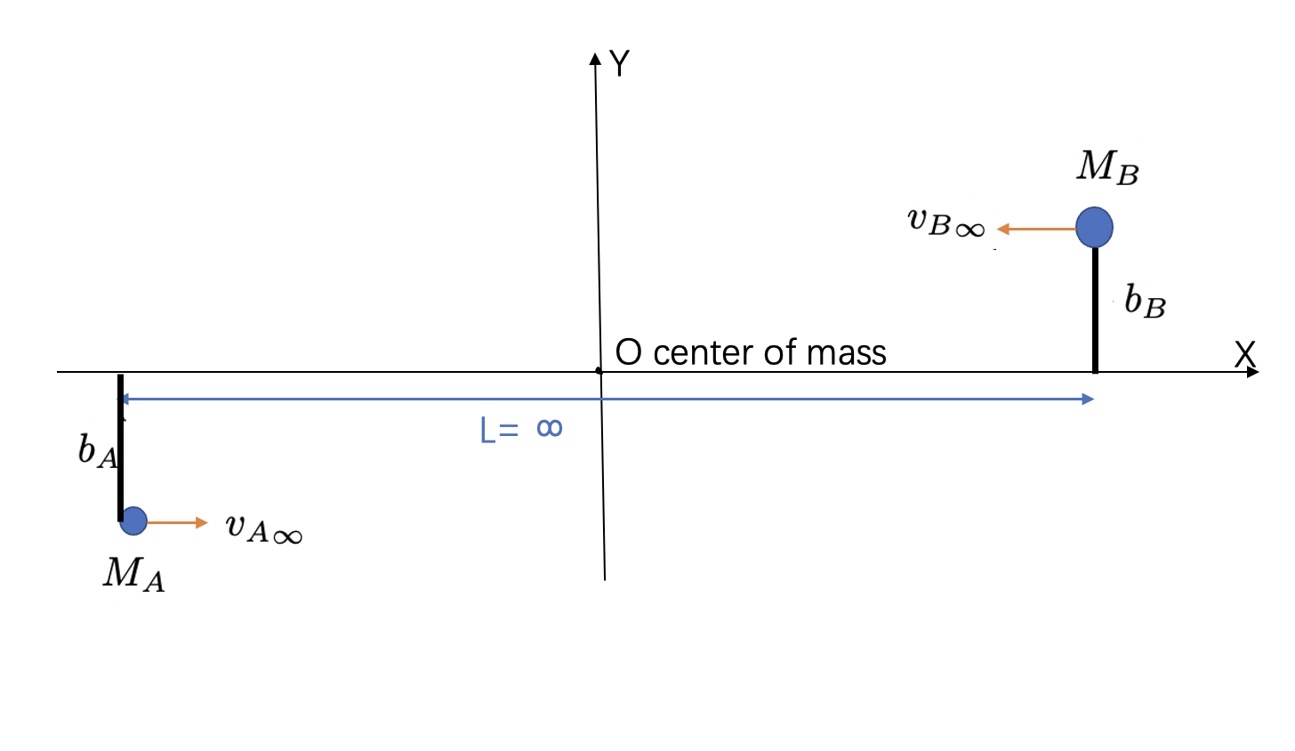
where we have defined . Additionally, we assume that the two points are initially at infinite distance, their relative speed is , and the impact parameter is . From Newtonian mechanics we know that the trajectory of each point is a hyperbola and the two points are moving in a plane (we set this plane as plane, and thus ), while the total energy of the system is positive. Additionally, the mass center of these two DM halos will not follow a hyperbolic trajectory at all times, in order to acquire a collision. In Fig. 1 we depict an illustrative representation of the initial conditions of the collision.
Let us start with the beginning of the collision, when the two DM halos start moving towards each other. For point A we have
| (10) |
where
| (11) | |||
| (12) | |||
| (13) |
We proceed by defining through
| (14) |
hence
| (15) | ||||
| (16) |
Note that corresponds to the time when the two mass points have the shortest distance.
In order to obtain the GW amplitude , we proceed to the calculation of the quadrupole moment and its second time derivative. We have
| (17) | |||||
| (18) | |||||
| (19) | ||||
| (20) | ||||
| (21) | ||||
| (22) |
and thus inserting into (18) we extract all the second time derivatives of the quadrupole moment , namely
For simplicity, we define , and the mass ratio . Noting that we have and , so that .
As a result, we get . Substitute the above equations into the formula of ,we have
| (26) | |||
| (27) | |||
| (28) |
We note that is independent from mass ratio , so . Besides, is also independent from mass ratio , so the is just equal to .In short, the mass ratio only affects by factors like .Therefore, we can get the results in any mass ratio from the equal mass result by the following equation,
| (29) |
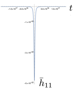
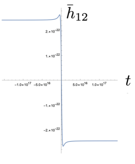
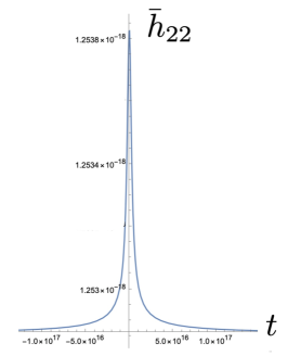
We can now use (3) in order to obtain the GW signal in the time domain. As typical values we set , namely the order of mass of a (dwarf) galaxy, where is the mass of the Sun, and we use , , which are the typical values for galaxy collisions. Moreover, we assume that the collision happens at a distance of from the Earth, which is roughly the distance of the source of GW150914. Hence, we can estimate the magnitude of the GW signal. In Fig. 2 we present the obtained dimensionless GW signal , as a function of time . Since corresponds to the time of shortest distance, the change rate of is fastest at this time, as expected. As we observe, the variation of is of the order of during the collision. However, this variation corresponds to a large time scale (about ), which implies that a single signal of this kind of GW is extremely hard to be detected. Additionally, we can see that the evolution of is faster than that of , , which implies that will be dominant in relatively higher frequency than that of , .
The GW amplitude in TT gauge is the traceless version of .We can project the GW amplitude in TT gauge by
| (30) | |||
| (31) | |||
| (32) | |||
| (33) |
while all other are equal to zero.
We proceed by taking the Fourier transformation of , in order to investigate its spectrum. In particular, we use
| (34) |
| (35) |
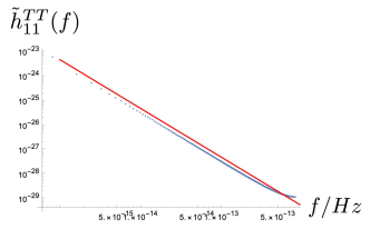
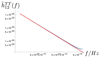
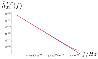
where , with the frequency. obey the power law in a very good approximation for a very wide frequency range. Besides, as , while , we can infer that will be dominant in the low frequency band while will be dominant in relatively high frequencies. In Fig. 3 we present the dependence of on .
3 Effect on the stochastic gravitational wave background
In this section, we calculate the contribution of the DM halos collisions to the stochastic gravitational wave background. Specifically, we integrate the gravitational wave spectrum of a single collision event over the number density of GW sources.
In principle, in order to compare a theoretical model with observations, one uses both the fractional energy density spectrum , as well as the characteristic strain amplitude Romano:2016dpx . They are related to the energy spectrum of GWB through the expression
| (36) |
where is the frequency of GW detected on Earth, and is the critical energy density. The energy spectrum of the stochastic GWB, , can be written as
| (37) |
with the redshift at the GW emission. Additionally, is the energy spectrum of a single GW event, which is calculated through the analysis of subsection 2, and is the GW frequency in the rest frame of GW sources, and thus .
We mention that we denote the parameters related to the number density of GW sources collectively by , and therefore is the number density of sources in the redshift interval and with source parameters in the interval . Hence, in the simple single event of two DM halos collision of the previous section we have , where , , and .
Let us now calculate the full distribution function . As we have checked numerically, the variance of has a minor effect on the final result, not affecting the order of magnitude. Hence, it is a good approximation to omit the change of , and consider that . Hence, we have
| (38) |
where the varying range of and is taken from Genel:2010pb .
In the following subsections we will separately calculate the energy spectrum of a single GW event , and the number density of GW sources .
3.1 Energy spectrum of a single GW event
The energy density of a single GW event can be calculated from the (traceless) second time derivative of the quadrupole moment, namely Maggiore:2018sht
| (39) |
where is the traceless quadrupole moment and is the Fourier transformation of the second time derivative of , which is related to via
| (40) | |||
| (41) | |||
| (42) | |||
| (43) |
while all other are equal to zero. Now, from Newtonian mechanics can be written as
| (44) |
where is the mass ratio of the two masses, and is defined as . Therefore, from the calculation of Section 2, we can extract the values of as
| (45) | |||
| (46) | |||
| (47) |
Hence, inserting the above into (39) gives us the energy density of a single GW event.
The energy density can be written as follows
| (48) |
where are constants. When , the contribution of to the energy spectrum can be ignored. In this case, the energy spectrum is consistent with the result in 2010gfe..book…..M which is given by:
| (49) |
It should be noted that integrating the energy spectrum of gravitational waves over the entire frequency range to determine the total energy released throughout the process will result in divergence.
The physical process of releasing high-frequency gravitational waves corresponds to two particles being very close together, causing rapid changes in the motion of particles. At this point, the release of gravitational waves will in turn have a significant impact on the motion of the two particles, rendering the approximation of elastic collision ineffective. Further more, it would even be unreasonable to consider the collision of dark matter halos as point particles under such circumstances.
Therefore, the frequency of the energy spectrum should be truncated at in order to avoid non-physical results. For and , the cutoff frequency .
3.2 Number density of GW sources
Let us now calculate the number density of GW sources (per redshift, total mass and mass ratio interval) . This number density is equal to the DM matter halos mergers rate, which can be calculated by combining the extended Press-Schechter (EPS) theory 2010gfe..book…..M and numerical simulations Genel:2010pb :
| (50) |
where is the number density of dark matter halos (per redshift per mass interval in the co-moving space), is a redshift-dependent function given below, and is the merger rate (at some ) for a pair of DM halos with fixed total mass and mass ratio . In the following we handle these terms separately.
We start with the definition of 2010gfe..book…..M
| (51) |
where is the linear growth rate of matter density. can be written as
| (52) |
where a good approximation of is
| (53) |
with , the density parameters of dark energy and matter sectors given by
| (54) |
where the normalized Hubble function reads as
| (55) |
with the value of the Hubble function at present time given as Planck:2018nkj
| (56) |
and with the values at present time taken as Planck:2018nkj
| (57) | |||
| (58) |
Note that in the above we consider that the underlying cosmology is CDM concordance scenario, i.e., the dark energy sector is the cosmological constant.
We continue by using the EPS theory in order to write the formula of the number density of DM halos . We consider that the halos merge when the redshift is between and , and that the emitted GW signals are detected at Earth at present. In co-moving space those halos are in the volume . Now, the EPS theory provides the number density of DM halos at some redshift and mass . Therefore, we have
| (59) |
where the radius in the co-moving space is 2010gfe..book…..M
| (60) |
while the formula of is 2010gfe..book…..M
| (61) |
In the above expression is the mean density of the matter component, , while is the variance of the matter density perturbation which can be estimated as 2010gfe..book…..M
| (62) |
with , , , , and , leading to
| (63) |
Finally, the last term of (50), namely (dimensionless since both are dimensionless), can be found in Genel:2010pb and it is given by
| (64) |
where the best-fit parameters from simulations are , , , , Genel:2010pb .
3.3 The energy spectrum of the stochastic gravitational wave background
We have now all the ingredients needed in order to calculate the energy spectrum of the stochastic gravitational wave background. This is given by (38), in which the energy spectrum of a single GW event was calculated in subsection 3.1, while the number density of GW sources was calculated in subsection 3.2. Assembling everything, we finally obtain the stochastic gravitational wave background resulting from DM halos collisions in the universe, which is calculated numerically and it is shown in Fig. 4. Besdies, instantaneous collision approximation introduce a cutoff frequency, the frequency beyond which the signal is truncated is the inverse of the timescale of the collision. The cutoff frequency for instantaneous collisions is . For the case of the dark matter halos collisions, This frequency is about .
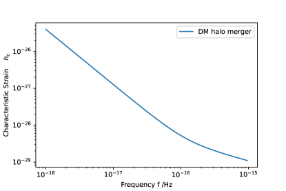
As we can see, the contribution of GW radiated from the collisions of DM halos, namely galaxies and galaxy clusters, is quite small comparing to other sources. In the pulsar timing array (PTA) band, where , and where the current observational limit is Burke-Spolaor:2018bvk . we obtain an effect of the order of in the band of . Nevertheless, in very low frequency band will be larger. In general, with current observational sensitivity the effect of the DM halos collisions on the stochastic gravitational wave background cannot be detectedTinto:2001ii ; Caprini:2019pxz ; Karnesis:2022vdp ; Chapman-Bird:2022tvu . Note that one could try to extend the analysis, by considering, instead of point masses, a group of mass points with Navarro, Frenk & White (NFW) density profile 2010gfe..book…..M to simulate DM halo collisions, nevertheless the results are expected to be at the same order of magnitude.
Dark matter halos are in reality extended objects and not point-particles. Strictly speaking, this two point toy model only suits for the beginning of the merger of 2 DM halos, at this stage the mechanical energy of the 2 mass centers of DM halo is approximately a constant. One may use N-body simulation to calculate the GW radiated from the merger more precisely. However, as an estimation of order of magnitude of the contribution to the GWB, the simple model in this paper is good enough.
4 Conclusions
In this work we investigated the effect of the dark matter halos collisions, namely collisions of galaxies and galaxy clusters, through gravitational bremsstrahlung, on the stochastic gravitational wave background.
In order to achieve this goal, we first calculated the gravitational wave signal of a single DM halo collision event. As an estimation of the order of magnitude, we handled the two DM halos as mass points. Furthermore, since the strength of such GW signals is weak, we adopted linear perturbation theory of General Relativity, namely we extracted the GW signal using the second time derivative of the quadruple moment. Additionally, since the velocity of DM halos is small, we applied non-relativistic Newtonian Mechanics. Hence, we extracted the GW signal through bremsstrahlung from a single DM halo collision. As we showed, is of the order of , and it becomes maximum at the time of shortest distance as expected. However, since such an event typically corresponds to duration of the order of , we deduce that a single signal of this kind of GW is extremely hard to be detected.
As a next step we proceeded to the calculation of the energy spectrum of the collective effect of all DM halos collisions in the Universe. This can arise by the energy spectrum of a GW signal radiated by a single collision, multiplied by the DM halo collision rate, and integrating over the whole Universe. Firstly, knowing the signal of a single collision we calculated its energy spectrum. Secondly, concerning the DM halo collision rate we showed that it is given by the product of the number density of DM halos, which is calculated by the EPS theory, with the collision rate of a single DM halo, which is given by simulation results, with a function of the linear growth rate of matter density through cosmological evolution. Hence, integrating over all mass and distance ranges, we finally extracted the spectrum of the stochastic gravitational wave background created by DM halos collisions.
As we show, the resulting contribution to the stochastic gravitational wave background is of the order of in the band of . However, in very low frequency band, is larger. With current observational sensitivity it cannot be detected.
In summary, with the current and future significant advance in gravitational-wave astronomy, and in particular with the tremendous improvement on the sensitivity bounds that Collaborations like Laser Interferometer Space Antenna (LISA), Einstein Telescope (ET), Cosmic Explorer (CE), etc will bring, it is both interesting and necessary to investigate all possible contributions to the stochastic gravitational wave background. And the gravitational bremsstrahlung during galaxies and galaxy clusters collisions is one of them.
Acknowledgments
We are grateful to Yifu Cai, Jiewen Chen, Zihan Zhou, Jiarui Li and Yumin Hu, Bo Wang and Rui Niu for helpful discussions. This work is supported in part by the National Key R&D Program of China (2021YFC2203100), by CAS young interdisciplinary innovation team (JCTD-2022-20), by the NSFC (12261131497), by 111 Project for “Observational and Theoretical Research on Dark Matter and Dark Energy” (B23042), by the Fundamental Research Funds for Central Universities, by the CSC Innovation Talent Funds, by the USTC Fellowship for International Cooperation, and by the USTC Research Funds of the Double First-Class Initiative. ENS acknowledges participation in the COST Association Action CA18108 “Quantum Gravity Phenomenology in the Multimessenger Approach (QG-MM)”. All numerics were operated on the computer clusters LINDA & JUDY in the particle cosmology group at USTC.
References
- (1) B.P. Abbott, et al., Phys. Rev. Lett. 116(6), 061102 (2016). DOI 10.1103/PhysRevLett.116.061102
- (2) B.P. Abbott, et al., Phys. Rev. Lett. 119(16), 161101 (2017). DOI 10.1103/PhysRevLett.119.161101
- (3) A. Goldstein, et al., Astrophys. J. Lett. 848(2), L14 (2017). DOI 10.3847/2041-8213/aa8f41
- (4) A. Addazi, et al., Prog. Part. Nucl. Phys. 125, 103948 (2022). DOI 10.1016/j.ppnp.2022.103948
- (5) R. Abbott, et al., Phys. Rev. X 11, 021053 (2021). DOI 10.1103/PhysRevX.11.021053
- (6) J.M. Ezquiaga, M. Zumalacárregui, Phys. Rev. Lett. 119(25), 251304 (2017). DOI 10.1103/PhysRevLett.119.251304
- (7) W. Zhao, L. Wen, Phys. Rev. D 97(6), 064031 (2018). DOI 10.1103/PhysRevD.97.064031
- (8) B.P. Abbott, et al., Astrophys. J. Lett. 848(2), L13 (2017). DOI 10.3847/2041-8213/aa920c
- (9) B.P. Abbott, et al., Nature 551(7678), 85 (2017). DOI 10.1038/nature24471
- (10) T. Baker, E. Bellini, P.G. Ferreira, M. Lagos, J. Noller, I. Sawicki, Phys. Rev. Lett. 119(25), 251301 (2017). DOI 10.1103/PhysRevLett.119.251301
- (11) G. Farrugia, J. Levi Said, V. Gakis, E.N. Saridakis, Phys. Rev. D 97(12), 124064 (2018). DOI 10.1103/PhysRevD.97.124064
- (12) Y.F. Cai, C. Li, E.N. Saridakis, L. Xue, Phys. Rev. D 97(10), 103513 (2018). DOI 10.1103/PhysRevD.97.103513
- (13) M. Hohmann, C. Pfeifer, J. Levi Said, U. Ualikhanova, Phys. Rev. D 99(2), 024009 (2019). DOI 10.1103/PhysRevD.99.024009
- (14) E.N. Saridakis, et al., (2021)
- (15) P. Amaro-Seoane, et al., Class. Quant. Grav. 29, 124016 (2012). DOI 10.1088/0264-9381/29/12/124016
- (16) P. Amaro-Seoane, et al., (2017)
- (17) T. Papanikolaou, JCAP 10, 089 (2022). DOI 10.1088/1475-7516/2022/10/089
- (18) G. Domènech, C. Lin, M. Sasaki, JCAP 04, 062 (2021). DOI 10.1088/1475-7516/2021/11/E01. [Erratum: JCAP 11, E01 (2021)]
- (19) L. Lentati, et al., Mon. Not. Roy. Astron. Soc. 453(3), 2576 (2015). DOI 10.1093/mnras/stv1538
- (20) Z. Arzoumanian, et al., Astrophys. J. Lett. 905(2), L34 (2020). DOI 10.3847/2041-8213/abd401
- (21) J.W. Chen, Y. Wang, Astrophys. J. 929(2), 168 (2022). DOI 10.3847/1538-4357/ac5bd4
- (22) J.W. Chen, Y. Zhang, Mon. Not. Roy. Astron. Soc. 481(2), 2249 (2018). DOI 10.1093/mnras/sty2268
- (23) J. Antoniadis, et al., Astron. Astrophys. 678, A48 (2023). DOI 10.1051/0004-6361/202346841
- (24) J. Antoniadis, et al., (2023)
- (25) N. Christensen, Rept. Prog. Phys. 82(1), 016903 (2019). DOI 10.1088/1361-6633/aae6b5
- (26) B.P. Abbott, et al., Phys. Rev. Lett. 116(13), 131102 (2016). DOI 10.1103/PhysRevLett.116.131102
- (27) B.J. Owen, L. Lindblom, C. Cutler, B.F. Schutz, A. Vecchio, N. Andersson, Phys. Rev. D 58, 084020 (1998). DOI 10.1103/PhysRevD.58.084020
- (28) A.H. Jaffe, D.C. Backer, Astrophys. J. 583, 616 (2003). DOI 10.1086/345443
- (29) N. Stergioulas, A. Bauswein, K. Zagkouris, H.T. Janka, Mon. Not. Roy. Astron. Soc. 418, 427 (2011). DOI 10.1111/j.1365-2966.2011.19493.x
- (30) J.A. Clark, A. Bauswein, N. Stergioulas, D. Shoemaker, Class. Quant. Grav. 33(8), 085003 (2016). DOI 10.1088/0264-9381/33/8/085003
- (31) F. De Lillo, J. Suresh, A.L. Miller, Mon. Not. Roy. Astron. Soc. 513(1), 1105 (2022). DOI 10.1093/mnras/stac984
- (32) D. Agarwal, J. Suresh, V. Mandic, A. Matas, T. Regimbau, Phys. Rev. D 106(4), 043019 (2022). DOI 10.1103/PhysRevD.106.043019
- (33) Y.T. Wang, Y. Cai, Z.G. Liu, Y.S. Piao, JCAP 01, 010 (2017). DOI 10.1088/1475-7516/2017/01/010
- (34) R. Flauger, N. Karnesis, G. Nardini, M. Pieroni, A. Ricciardone, J. Torrado, JCAP 01, 059 (2021). DOI 10.1088/1475-7516/2021/01/059
- (35) N. Bellomo, D. Bertacca, A.C. Jenkins, S. Matarrese, A. Raccanelli, T. Regimbau, A. Ricciardone, M. Sakellariadou, JCAP 06(06), 030 (2022). DOI 10.1088/1475-7516/2022/06/030
- (36) Z. Zhao, Y. Di, L. Bian, R.G. Cai, (2022)
- (37) M. Maggiore, Phys. Rept. 331, 283 (2000). DOI 10.1016/S0370-1573(99)00102-7
- (38) K.N. Ananda, C. Clarkson, D. Wands, Phys. Rev. D 75, 123518 (2007). DOI 10.1103/PhysRevD.75.123518
- (39) C. Caprini, D.G. Figueroa, Class. Quant. Grav. 35(16), 163001 (2018). DOI 10.1088/1361-6382/aac608
- (40) I. Musco, J.C. Miller, Class. Quant. Grav. 30, 145009 (2013). DOI 10.1088/0264-9381/30/14/145009
- (41) T. Papanikolaou, C. Tzerefos, S. Basilakos, E.N. Saridakis, JCAP 10, 013 (2022). DOI 10.1088/1475-7516/2022/10/013
- (42) T. Papanikolaou, C. Tzerefos, S. Basilakos, E.N. Saridakis, Eur. Phys. J. C 83(1), 31 (2023). DOI 10.1140/epjc/s10052-022-11157-4
- (43) S. Banerjee, T. Papanikolaou, E.N. Saridakis, Phys. Rev. D 106(12), 124012 (2022). DOI 10.1103/PhysRevD.106.124012
- (44) T. Papanikolaou, V. Vennin, D. Langlois, JCAP 03, 053 (2021). DOI 10.1088/1475-7516/2021/03/053
- (45) J.F. Dufaux, A. Bergman, G.N. Felder, L. Kofman, J.P. Uzan, Phys. Rev. D 76, 123517 (2007). DOI 10.1103/PhysRevD.76.123517
- (46) Y.f. Cai, Y.S. Piao, Phys. Lett. B 657, 1 (2007). DOI 10.1016/j.physletb.2007.09.068
- (47) S. Kuroyanagi, T. Chiba, N. Sugiyama, Phys. Rev. D 79, 103501 (2009). DOI 10.1103/PhysRevD.79.103501
- (48) N.E. Mavromatos, J. Solà Peracaula, Eur. Phys. J. ST 230(9), 2077 (2021). DOI 10.1140/epjs/s11734-021-00197-8
- (49) Z. Zhou, J. Jiang, Y.F. Cai, M. Sasaki, S. Pi, Phys. Rev. D 102(10), 103527 (2020). DOI 10.1103/PhysRevD.102.103527
- (50) A. Achúcarro, et al., (2022)
- (51) M. Zhu, A. Ilyas, Y. Zheng, Y.F. Cai, E.N. Saridakis, JCAP 11(11), 045 (2021). DOI 10.1088/1475-7516/2021/11/045
- (52) Y.F. Cai, X.H. Ma, M. Sasaki, D.G. Wang, Z. Zhou, JCAP 12, 034 (2022). DOI 10.1088/1475-7516/2022/12/034
- (53) G. Franciolini, I. Musco, P. Pani, A. Urbano, Phys. Rev. D 106(12), 123526 (2022). DOI 10.1103/PhysRevD.106.123526
- (54) A. Addazi, S. Capozziello, Q. Gan, JCAP 08(08), 051 (2022). DOI 10.1088/1475-7516/2022/08/051
- (55) N.E. Mavromatos, V.C. Spanos, I.D. Stamou, Phys. Rev. D 106(6), 063532 (2022). DOI 10.1103/PhysRevD.106.063532
- (56) S. Kazempour, A.R. Akbarieh, E.N. Saridakis, Phys. Rev. D 106(10), 103502 (2022). DOI 10.1103/PhysRevD.106.103502
- (57) T. Papanikolaou, A. Lymperis, S. Lola, E.N. Saridakis, JCAP 03, 003 (2023). DOI 10.1088/1475-7516/2023/03/003
- (58) B. Allen, J.D. Romano, Phys. Rev. D 59, 102001 (1999). DOI 10.1103/PhysRevD.59.102001
- (59) S. Capozziello, M. De Laurentis, S. Nojiri, S.D. Odintsov, Gen. Rel. Grav. 41, 2313 (2009). DOI 10.1007/s10714-009-0758-1
- (60) A. Sesana, A. Vecchio, C.N. Colacino, Mon. Not. Roy. Astron. Soc. 390, 192 (2008). DOI 10.1111/j.1365-2966.2008.13682.x
- (61) J.D. Romano, N.J. Cornish, Living Rev. Rel. 20(1), 2 (2017). DOI 10.1007/s41114-017-0004-1
- (62) P. Huang, A.J. Long, L.T. Wang, Phys. Rev. D 94(7), 075008 (2016). DOI 10.1103/PhysRevD.94.075008
- (63) R.G. Cai, T.B. Liu, X.W. Liu, S.J. Wang, T. Yang, Phys. Rev. D 97(10), 103005 (2018). DOI 10.1103/PhysRevD.97.103005
- (64) Y.F. Cai, C. Chen, X. Tong, D.G. Wang, S.F. Yan, Phys. Rev. D 100(4), 043518 (2019). DOI 10.1103/PhysRevD.100.043518
- (65) T. Regimbau, Symmetry 14(2), 270 (2022). DOI 10.3390/sym14020270
- (66) Z. Arzoumanian, et al., Astrophys. J. 859(1), 47 (2018). DOI 10.3847/1538-4357/aabd3b
- (67) L. Speri, N. Karnesis, A.I. Renzini, J.R. Gair, Nature Astron. 6(12), 1356 (2022). DOI 10.1038/s41550-022-01849-y
- (68) M. Georgousi, N. Karnesis, V. Korol, M. Pieroni, N. Stergioulas, Mon. Not. Roy. Astron. Soc. 519(2), 2552 (2022). DOI 10.1093/mnras/stac3686
- (69) G. Agazie, et al., Astrophys. J. Lett. 952(2), L37 (2023). DOI 10.3847/2041-8213/ace18b
- (70) N. Aghanim, et al., Astron. Astrophys. 641, A1 (2020). DOI 10.1051/0004-6361/201833880
- (71) N. Aghanim, et al., Astron. Astrophys. 641, A6 (2020). DOI 10.1051/0004-6361/201833910. [Erratum: Astron.Astrophys. 652, C4 (2021)]
- (72) P.A.R. Ade, et al., Astron. Astrophys. 571, A16 (2014). DOI 10.1051/0004-6361/201321591
- (73) G. Bertone, D. Hooper, J. Silk, Phys. Rept. 405, 279 (2005). DOI 10.1016/j.physrep.2004.08.031
- (74) G. Jungman, M. Kamionkowski, K. Griest, Phys. Rept. 267, 195 (1996). DOI 10.1016/0370-1573(95)00058-5
- (75) J. Preskill, M.B. Wise, F. Wilczek, Phys. Lett. B 120, 127 (1983). DOI 10.1016/0370-2693(83)90637-8
- (76) N. Arkani-Hamed, D.P. Finkbeiner, T.R. Slatyer, N. Weiner, Phys. Rev. D 79, 015014 (2009). DOI 10.1103/PhysRevD.79.015014
- (77) V.C. Rubin, N. Thonnard, W.K. Ford, Jr., Astrophys. J. 238, 471 (1980). DOI 10.1086/158003
- (78) D. Clowe, M. Bradac, A.H. Gonzalez, M. Markevitch, S.W. Randall, C. Jones, D. Zaritsky, Astrophys. J. Lett. 648, L109 (2006). DOI 10.1086/508162
- (79) J.F. Navarro, C.S. Frenk, S.D.M. White, Astrophys. J. 462, 563 (1996). DOI 10.1086/177173
- (80) M. Davis, G. Efstathiou, C.S. Frenk, S.D.M. White, Astrophys. J. 292, 371 (1985). DOI 10.1086/163168
- (81) S.D.M. White, M.J. Rees, Mon. Not. Roy. Astron. Soc. 183, 341 (1978). DOI 10.1093/mnras/183.3.341
- (82) J.S. Bullock, T.S. Kolatt, Y. Sigad, R.S. Somerville, A.V. Kravtsov, A.A. Klypin, J.R. Primack, A. Dekel, Mon. Not. Roy. Astron. Soc. 321, 559 (2001). DOI 10.1046/j.1365-8711.2001.04068.x
- (83) P.C. Peters, Phys. Rev. D 1, 1559 (1970). DOI 10.1103/PhysRevD.1.1559
- (84) R.J. Crowley, K.S. Thorne, Astrophys. J. 215, 624 (1977). DOI 10.1086/155397
- (85) L. Smarr, Phys. Rev. D 15, 2069 (1977). DOI 10.1103/PhysRevD.15.2069
- (86) S.J. Kovacs, K.S. Thorne, Astrophys. J. 224, 62 (1978). DOI 10.1086/156350
- (87) B.D. Farris, Y.T. Liu, S.L. Shapiro, Phys. Rev. D 84, 024024 (2011). DOI 10.1103/PhysRevD.84.024024
- (88) S. Mougiakakos, M.M. Riva, F. Vernizzi, Phys. Rev. D 104(2), 024041 (2021). DOI 10.1103/PhysRevD.104.024041
- (89) E. Herrmann, J. Parra-Martinez, M.S. Ruf, M. Zeng, Phys. Rev. Lett. 126(20), 201602 (2021). DOI 10.1103/PhysRevLett.126.201602
- (90) S. Mougiakakos, M.M. Riva, F. Vernizzi, Phys. Rev. Lett. 129(12), 121101 (2022). DOI 10.1103/PhysRevLett.129.121101
- (91) G.U. Jakobsen, G. Mogull, J. Plefka, J. Steinhoff, Phys. Rev. Lett. 128(1), 011101 (2022). DOI 10.1103/PhysRevLett.128.011101
- (92) L. Gondán, B. Kocsis, Mon. Not. Roy. Astron. Soc. 515(3), 3299 (2022). DOI 10.1093/mnras/stac1985
- (93) M.M. Riva, F. Vernizzi, L.K. Wong, Phys. Rev. D 106(4), 044013 (2022). DOI 10.1103/PhysRevD.106.044013
- (94) T. Inagaki, K. Takahashi, S. Masaki, N. Sugiyama, Phys. Rev. D 82, 124007 (2010). DOI 10.1103/PhysRevD.82.124007
- (95) T. Inagaki, K. Takahashi, N. Sugiyama, Phys. Rev. D 85, 104051 (2012). DOI 10.1103/PhysRevD.85.104051
- (96) H. Mo, F.C. van den Bosch, S. White, Galaxy Formation and Evolution (2010)
- (97) M. Maggiore, Gravitational Waves. Vol. 1: Theory and Experiments. Oxford Master Series in Physics (Oxford University Press, 2007)
- (98) S. Genel, N. Bouche, T. Naab, A. Sternberg, R. Genzel, Astrophys. J. 719, 229 (2010). DOI 10.1088/0004-637X/719/1/229
- (99) M. Maggiore, Gravitational Waves. Vol. 2: Astrophysics and Cosmology (Oxford University Press, 2018)
- (100) S. Burke-Spolaor, et al., Astron. Astrophys. Rev. 27(1), 5 (2019). DOI 10.1007/s00159-019-0115-7
- (101) M. Tinto, J.W. Armstrong, F.B. Estabrook, Phys. Rev. D 63, 021101 (2001). DOI 10.1103/PhysRevD.63.021101
- (102) C. Caprini, D.G. Figueroa, R. Flauger, G. Nardini, M. Peloso, M. Pieroni, A. Ricciardone, G. Tasinato, JCAP 11, 017 (2019). DOI 10.1088/1475-7516/2019/11/017
- (103) N. Karnesis, et al., (2022)
- (104) C.E.A. Chapman-Bird, C.P.L. Berry, G. Woan, Mon. Not. Roy. Astron. Soc. 522(4), 6043 (2023). DOI 10.1093/mnras/stad1397