This paper was converted on www.awesomepapers.org from LaTeX by an anonymous user.
Want to know more? Visit the Converter page.

Stochastic Approximation Approaches to
Group Distributionally Robust Optimization and Beyond

\nameLijun Zhang \email[email protected] \AND\nameHaomin Bai \email[email protected] \AND\namePeng Zhao \email[email protected]
\addrNational Key Laboratory for Novel Software Technology, Nanjing University, China
School of Artificial Intelligence, Nanjing University, China \AND\nameTianbao Yang \email[email protected]
\addrDepartment of Computer Science and Engineering, Texas A&\&M University, College Station, USA \AND\nameZhi-Hua Zhou \email[email protected]
\addrNational Key Laboratory for Novel Software Technology, Nanjing University, China
School of Artificial Intelligence, Nanjing University, China
Abstract

This paper investigates group distributionally robust optimization (GDRO) with the goal of learning a model that performs well over mm different distributions. First, we formulate GDRO as a stochastic convex-concave saddle-point problem, which is then solved by stochastic mirror descent (SMD) with mm samples in each iteration, and attain a nearly optimal sample complexity. To reduce the number of samples required in each round from mm to 1, we cast GDRO as a two-player game, where one player conducts SMD and the other executes an online algorithm for non-oblivious multi-armed bandits, maintaining the same sample complexity. Next, we extend GDRO to address scenarios involving imbalanced data and heterogeneous distributions. In the first scenario, we introduce a weighted variant of GDRO, enabling distribution-dependent convergence rates that rely on the number of samples from each distribution. We design two strategies to meet the sample budget: one integrates non-uniform sampling into SMD, and the other employs the stochastic mirror-prox algorithm with mini-batches, both of which deliver faster rates for distributions with more samples. In the second scenario, we propose to optimize the average top-kk risk instead of the maximum risk, thereby mitigating the impact of outlier distributions. Similar to the case of vanilla GDRO, we develop two stochastic approaches: one uses mm samples per iteration via SMD, and the other consumes kk samples per iteration through an online algorithm for non-oblivious combinatorial semi-bandits.

Keywords: Group distributionally robust optimization (GDRO), Stochastic convex-concave saddle-point problem, Non-oblivious online learning, Bandits, Average top-kk risk

1 Introduction

In the classical statistical machine learning, our goal is to minimize the risk with respect to a fixed distribution 𝒫0\mathcal{P}_{0} (Vapnik, 2000), i.e.,

min𝐰𝒲{R0(𝐰)=E𝐳𝒫0[(𝐰;𝐳)]},\min_{\mathbf{w}\in\mathcal{W}}\ \left\{R_{0}(\mathbf{w})=\mathrm{E}_{\mathbf{z}\sim\mathcal{P}_{0}}\big{[}\ell(\mathbf{w};\mathbf{z})\big{]}\right\}, (1)

where 𝐳𝒵\mathbf{z}\in\mathcal{Z} is a sample drawn from 𝒫0\mathcal{P}_{0}, 𝒲\mathcal{W} denotes a hypothesis class, and (𝐰;𝐳)\ell(\mathbf{w};\mathbf{z}) is a loss measuring the prediction error of model 𝐰\mathbf{w} on 𝐳\mathbf{z}. During the past decades, various algorithms have been developed to optimize (1), and can be grouped in two categories: sample average approximation (SAA) and stochastic approximation (SA) (Kushner and Yin, 2003). In SAA, we minimize an empirical risk defined as the average loss over a set of samples drawn from 𝒫0\mathcal{P}_{0}, and in SA, we directly solve the original problem by using stochastic observations of the objective R0()R_{0}(\cdot).

However, a model trained on a single distribution may lack robustness in the sense that (i) it could suffer high error on minority subpopulations, though the average loss is small; (ii) its performance could degenerate dramatically when tested on a different distribution. Distributionally robust optimization (DRO) provides a principled way to address those limitations by minimizing the worst-case risk in a neighborhood of 𝒫0\mathcal{P}_{0} (Ben-Tal et al., 2013). Recently, it has attracted great interest in optimization (Shapiro, 2017), statistics (Duchi and Namkoong, 2021), operations research (Duchi et al., 2021), and machine learning (Hu et al., 2018; Curi et al., 2020; Jin et al., 2021; Agarwal and Zhang, 2022). In this paper, we consider an emerging class of DRO problems, named as Group DRO (GDRO) which optimizes the maximum risk

max(𝐰)=maxi[m]{Ri(𝐰)=E𝐳𝒫i[(𝐰;𝐳)]}\mathcal{L}_{\max}(\mathbf{w})=\max_{i\in[m]}\left\{R_{i}(\mathbf{w})=\mathrm{E}_{\mathbf{z}\sim\mathcal{P}_{i}}\big{[}\ell(\mathbf{w};\mathbf{z})\big{]}\right\} (2)

over a finite number of distributions (Oren et al., 2019; Sagawa et al., 2020). Mathematically, GDRO can be formulated as a minimax stochastic problem:

min𝐰𝒲maxi[m]{Ri(𝐰)}\min_{\mathbf{w}\in\mathcal{W}}\max_{i\in[m]}\ \left\{R_{i}(\mathbf{w})\right\} (3)

where 𝒫1,,𝒫m\mathcal{P}_{1},\ldots,\mathcal{P}_{m} denote mm distributions. A motivating example is federated learning, where a centralized model is deployed at multiple clients, each of which faces a (possibly) different data distribution (Mohri et al., 2019).

Supposing that samples can be drawn from all distributions freely, we develop efficient SA approaches for (3), in favor of their light computations over SAA methods. As elaborated by Nemirovski et al. (2009, § 3.2), we can cast (3) as a stochastic convex-concave saddle-point problem:

min𝐰𝒲max𝐪Δm{ϕ(𝐰,𝐪)=i=1mqiRi(𝐰)}\min_{\mathbf{w}\in\mathcal{W}}\max_{\mathbf{q}\in\Delta_{m}}\ \left\{\phi(\mathbf{w},\mathbf{q})=\sum_{i=1}^{m}q_{i}R_{i}(\mathbf{w})\right\} (4)

where Δm={𝐪m|𝐪𝟎,i=1mqi=1}\Delta_{m}=\{\mathbf{q}\in\mathbb{R}^{m}|\mathbf{q}\geq\mathbf{0},\sum_{i=1}^{m}q_{i}=1\} is the (m1m{-}1)-dimensional simplex, and then solve (4) by their mirror descent stochastic approximation method, namely stochastic mirror descent (SMD). In fact, several recent studies have adopted this (or similar) strategy to optimize (4). But, unfortunately, we found that existing results are unsatisfactory because they either deliver a loose sample complexity (Sagawa et al., 2020), suffer subtle dependency issues in their analysis (Haghtalab et al., 2022; Soma et al., 2022), or hold only in expectation (Carmon and Hausler, 2022).

As a starting point, we first provide a routine application of SMD to (4), and discuss the theoretical guarantee. In each iteration, we draw 11 sample from every distribution to construct unbiased estimators of Ri()R_{i}(\cdot) and its gradient, and then update both 𝐰\mathbf{w} and 𝐪\mathbf{q} by SMD. The proposed method achieves an O((logm)/T)O(\sqrt{(\log m)/T}) convergence rate in expectation and with high probability, where TT is the total number of iterations. As a result, we obtain an O(m(logm)/ϵ2)O(m(\log m)/\epsilon^{2}) sample complexity for finding an ϵ\epsilon-optimal solution of (4), which matches the Ω(m/ϵ2)\Omega(m/\epsilon^{2}) lower bound (Soma et al., 2022, Theorem 5) up to a logarithmic factor, and tighter than the O(m2(logm)/ϵ2)O(m^{2}(\log m)/\epsilon^{2}) bound of Sagawa et al. (2020) by an mm factor. While being straightforward, this result seems new for GDRO. Additionally, we note that the aforementioned method requires setting the number of iterations TT in advance, which could be inconvenient in practice. To avoid this limitation, we further propose an anytime algorithm by using time-varying step sizes, and obtain an O~((logm)/t)\widetilde{O}(\sqrt{(\log m)/t}) 111We use the O~\widetilde{O} notation to hide constant factors as well as polylogarithmic factors in tt. convergence rate at each iteration tt.

Then, we proceed to reduce the number of samples used in each iteration from mm to 11. We remark that a naive uniform sampling over mm distributions does not work well, and yields a higher sample complexity (Sagawa et al., 2020). As an alternative, we borrow techniques from online learning with stochastic observations, and explicitly tackle the non-oblivious nature of the online process, which distinguishes our method from that of Soma et al. (2022). Specifically, we use SMD to update 𝐰\mathbf{w}, and Exp3-IX, a powerful algorithm for non-oblivious multi-armed bandits (MAB) (Neu, 2015), with stochastic rewards to update 𝐪\mathbf{q}. In this way, our algorithm only needs 11 sample in each round and attains an O(m(logm)/T)O(\sqrt{m(\log m)/T}) convergence rate, implying the same O(m(logm)/ϵ2)O(m(\log m)/\epsilon^{2}) sample complexity. Similarly, we also put forward an anytime variant, achieving an O~(m(logm)/t)\widetilde{O}(\sqrt{m(\log m)/t}) convergence rate.

Subsequently, we extend GDRO to address two specific scenarios, as illustrated below.

1.1 Extension to Imbalanced Data

In the first extention, we investigate a more practical and challenging scenario in which there are different budgets of samples that can be drawn from each distribution, a natural phenomenon encountered in learning with imbalanced data (Amodei et al., 2016). Let nin_{i} be the sample budget of the ii-th distribution, and without loss of generality, we assume that n1n2nmn_{1}\geq n_{2}\geq\cdots\geq n_{m}. Now, the goal is not to attain the optimal sample complexity, but to reduce the risk on all distributions as much as possible, under the budget constraint. To achieve this goal, we propose a novel formulation of weighted GDRO, which weights each risk Ri()R_{i}(\cdot) in (4) by a scale factor pip_{i}. For GDRO with different budgets, we develop two SA approaches based on non-uniform sampling and mini-batches, respectively.

In each iteration of the first approach, we draw 11 sample from every 𝒫i\mathcal{P}_{i} with probability ni/n1n_{i}/n_{1}, and then construct stochastic gradients to perform mirror descent. Consequently, the budget will be satisfied in expectation after n1n_{1} rounds, and our algorithm can be regarded as SMD for an instance of weighted GDRO. With the help of scale factors, we demonstrate the proposed algorithm enjoys distribution-dependent convergence in the sense that it converges faster for distributions with more samples. In particular, the excess risk on distribution 𝒫i\mathcal{P}_{i} reduces at an O(n1logm/ni)O(\sqrt{n_{1}\log m}/n_{i}) rate, and for 𝒫1\mathcal{P}_{1}, it becomes O((logm)/n1)O(\sqrt{(\log m)/n_{1}}), which almost matches the optimal O(1/n1)O(\sqrt{1/n_{1}}) rate of learning from a single distribution with n1n_{1} samples.

On the other hand, for distribution 𝒫i\mathcal{P}_{i} with budget ni<n1n_{i}<n_{1}, the above O(n1logm/ni)O(\sqrt{n_{1}\log m}/n_{i}) rate is worse than the O(1/ni)O(\sqrt{1/n_{i}}) rate obtained by learning from 𝒫i\mathcal{P}_{i} alone. In shape contrast with this limitation, our second approach yields nearly optimal convergence rates for multiple distributions across a large range of budgets. To meet the budget constraint, it runs for n¯nm\bar{n}\leq n_{m} rounds, and in each iteration, draws a mini-batch of ni/n¯n_{i}/\bar{n} samples from every distribution 𝒫i\mathcal{P}_{i}. As a result, (i) the budget constraint is satisfied exactly; (ii) for distributions with a larger budget, the associated risk function can be estimated more accurately, making the variance of the stochastic gradient smaller. To benefit from the small variance, we leverage stochastic mirror-prox algorithm (Juditsky et al., 2011), instead of SMD, to update solutions, and again make use of the weighted GDRO formulation to obtain distribution-wise convergence rates. Theoretical analysis shows that the excess risk converges at an O((1nm+1ni)logm)O((\frac{1}{n_{m}}+\frac{1}{\sqrt{n_{i}}})\log m) rate for each 𝒫i\mathcal{P}_{i}. Thus, we obtain a nearly optimal O((logm)/ni)O((\log m)/\sqrt{n_{i}}) rate for distributions 𝒫i\mathcal{P}_{i} with ninm2n_{i}\leq n_{m}^{2}, and an O((logm)/nm)O((\log m)/n_{m}) rate otherwise. Note that the latter rate is as expected since the algorithm only updates O(nm)O(n_{m}) times.

1.2 Extension to Heterogeneous Distributions

In the second extension, we delve into another scenario where distributions exhibit heterogeneity, indicating significant variations in their risks (Li et al., 2019). The widely acknowledged sensitivity of the max operation to outliers implies that GDRO could be dominated by a single outlier distribution, while neglecting others (Shalev-Shwartz and Wexler, 2016). Inspired by the average top-kk loss for supervised learning (Fan et al., 2017), we modify our objective from the maximum risk max(𝐰)\mathcal{L}_{\max}(\mathbf{w}) in GDRO to the average top-kk risk:

k(𝐰)=maxm,k{1kiRi(𝐰)}\mathcal{L}_{k}(\mathbf{w})=\max_{\mathcal{I}\in\mathcal{B}_{m,k}}\left\{\frac{1}{k}\sum_{i\in\mathcal{I}}R_{i}(\mathbf{w})\right\} (5)

where m,k\mathcal{B}_{m,k} is the set of subsets of [m][m] with size kk, i.e., m,k={[m]|||=k}\mathcal{B}_{m,k}=\{\mathcal{I}\subseteq[m]||\mathcal{I}|=k\}. This modification aims to reduce the impact of outliers in heterogeneous distributions while still including GDRO as a special case.

We refer to the minimization of k(𝐰)\mathcal{L}_{k}(\mathbf{w}) as average top-kk risk optimization (ATkRO), and develop two stochastic algorithms. Similar to GDRO, ATkRO can be formulated as a stochastic convex-concave saddle-point problem, akin to (4), with the only difference being that the domain of 𝐪\mathbf{q} is the capped simplex instead of the standard simplex. Therefore, we can employ SMD to update 𝐰\mathbf{w} and 𝐪\mathbf{q}, which uses mm samples in each round. Theoretical analysis demonstrates that this approach achieves an O((log(m/k))/T)O(\sqrt{(\log(m/k))/T}) convergence rate, implying an O((mlog(m/k))/ϵ2)O((m\log(m/k))/\epsilon^{2}) sample complexity. Furthermore, to circumvent the limitation of predefining the total number of iterations TT, we introduce an anytime version that attains an O~((log(m/k))/t)\widetilde{O}(\sqrt{(\log(m/k))/t}) convergence rate.

Following the second approach for GDRO, we reduce the number of samples required in each round from mm to kk by casting ATkRO as a two-player game. In each round, we use the Dependent Rounding (DepRound) algorithm (Gandhi et al., 2006) to select kk distributions based on the current value of 𝐪\mathbf{q}, and then draw 11 sample from each selected distribution. Then, we construct unbiased stochastic gradients for 𝐰\mathbf{w}, and apply SMD for updates. Since the domain of 𝐪\mathbf{q} is the capped simplex, we model the online problem for 𝐪\mathbf{q} as an instance of non-oblivious combinatorial semi-bandits, and extend Exp3-IX to develop its update rule. We prove that our algorithm achieves an O(m(logm)/(kT))O(\sqrt{m(\log m)/(kT)}) convergence rate, yielding an O(m(logm)/ϵ2)O(m(\log m)/\epsilon^{2}) sample complexity. Similarly, we have also designed an anytime approach, which uses 11 sample per round and achieves an O~(m(logm)/t)\widetilde{O}(\sqrt{m(\log m)/t}) rate.

This paper extends our previous conference version (Zhang et al., 2023) by developing anytime algorithms, investigating a new scenario, and conducting more experiments, as detailed below.

  • First, we adapt the two SA algorithms for GDRO to operate in an anytime manner. In the conference paper, our algorithms for GDRO required predefining the total number of iterations TT to set step sizes. By adopting time-varying step sizes, we design anytime algorithms and provide the corresponding theoretical analysis.

  • Second, we explore the scenario of heterogeneous distributions, which involves outlier distributions with significantly high risks. To mitigate the impact of these outliers, we propose to solve the ATkRO problem and develop two algorithms: one employs SMD with mm samples per round, achieving a sample complexity of O((mlog(m/k))/ϵ2)O((m\log(m/k))/\epsilon^{2}); the other combines SMD with an algorithm for non-oblivious combinatorial semi-bandits, achieving a sample complexity of O(m(logm)/ϵ2)O(m(\log m)/\epsilon^{2}) and using kk samples in each iteration. Furthermore, we have also extended these two algorithms into anytime versions.

  • Last, we construct a heterogeneous data set and perform experiments to verify the advantages of ATkRO. Additionally, we compare the performance of the anytime algorithms with their non-anytime counterparts, demonstrating the benefits of the anytime capability.

2 Related Work

Distributionally robust optimization (DRO) stems from the pioneering work of Scarf (1958), and has gained a lot of interest with the advancement of robust optimization (Ben-Tal et al., 2009, 2015). It has been successfully applied to a variety of machine learning tasks, including adversarial training (Sinha et al., 2018), algorithmic fairness (Hashimoto et al., 2018), class imbalance (Xu et al., 2020), long-tail learning (Samuel and Chechik, 2021), label shift (Zhang et al., 2021), etc.

In general, DRO is formulated to reflect our uncertainty about the target distribution. To ensure good performance under distribution perturbations, it minimizes the risk w.r.t. the worst distribution in an uncertainty set, i.e.,

min𝐰𝒲sup𝒫SS(𝒫0){E𝐳𝒫[(𝐰;𝐳)]}\min_{\mathbf{w}\in\mathcal{W}}\ \sup_{\mathcal{P}\in\SS(\mathcal{P}_{0})}\left\{\mathrm{E}_{\mathbf{z}\sim\mathcal{P}}\big{[}\ell(\mathbf{w};\mathbf{z})\big{]}\right\} (6)

where SS(𝒫0)\SS(\mathcal{P}_{0}) denotes a set of probability distributions around 𝒫0\mathcal{P}_{0}. In the literature, there mainly exist three ways to construct SS(𝒫0)\SS(\mathcal{P}_{0}): (i) enforcing moment constraints (Delage and Ye, 2010), (ii) defining a neighborhood around 𝒫0\mathcal{P}_{0} by a distance function such as the ff-divergence (Ben-Tal et al., 2013), the Wasserstein distance (Kuhn et al., 2019), and the Sinkhorn distance (Wang et al., 2021), and (iii) hypothesis testing of goodness-of-fit (Bertsimas et al., 2018).

By drawing a set of samples from 𝒫0\mathcal{P}_{0}, we can also define an empirical DRO problem, which can be regarded as an SAA approach for solving (6). When the uncertainty set is defined in terms of the Cressie–Read family of ff-divergences, Duchi and Namkoong (2021) have studied finite sample and asymptotic properties of the empirical solution. Besides, it has been proved that empirical DRO can also benefit the risk minimization problem in (1). Namkoong and Duchi (2017) show that empirical DRO with the χ2\chi^{2}-divergence has the effect of variance regularization, leading to better generalization w.r.t. distribution 𝒫0\mathcal{P}_{0}. Later, Duchi et al. (2021) demonstrate similar behaviors for the ff-divergence constrained neighborhood, and provide one- and two-sided confidence intervals for the minimum risk in (1). Based on the Wasserstein distance, Esfahani and Kuhn (2018) establish an upper confidence bound on the risk of the empirical solution.

Since (6) is more complex than (1), considerable research efforts were devoted to develop efficient algorithms for DRO and its empirical version. For 𝒫0\mathcal{P}_{0} with finite support, Ben-Tal et al. (2013, Corollary 3) have demonstrated that (6) with ff-divergences is equivalent to a convex optimization problem, provided that the loss (𝐰;𝐳)\ell(\mathbf{w};\mathbf{z}) is convex in 𝐰\mathbf{w}. Actually, this conclusion is true even when 𝒫0\mathcal{P}_{0} is continuous (Shapiro, 2017, § 3.2). Under mild assumptions, Esfahani and Kuhn (2018) show that DRO problems over Wasserstein balls can be reformulated as finite convex programs—in some cases even as linear programs. Besides the constrained formulation in (6), there also exists a penalized (or regularized) form of DRO (Sinha et al., 2018), which makes the optimization problem more tractable. In the past years, a series of SA methods have been proposed for empirical DRO with convex losses (Namkoong and Duchi, 2016), and DRO with convex loss (Levy et al., 2020) and non-convex losses (Jin et al., 2021; Qi et al., 2021; Rafique et al., 2022).

The main focus of this paper is the GDRO problem in (3)/(4), instead of the traditional DRO in (6). Sagawa et al. (2020) have applied SMD (Nemirovski et al., 2009) to (4), but only obtain a sub-optimal sample complexity of O(m2(logm)/ϵ2)O(m^{2}(\log m)/\epsilon^{2}), because of the large variance in their gradients. In the sequel, Haghtalab et al. (2022) and Soma et al. (2022) have tried to improve the sample complexity by reusing samples and applying techniques from MAB respectively, but their analysis suffers dependency issues. Carmon and Hausler (2022, Proposition 2) successfully established an O(m(logm)/ϵ2)O(m(\log m)/\epsilon^{2}) sample complexity by combining SMD and gradient clipping, but their result holds only in expectation. To deal with heterogeneous noise in different distributions, Agarwal and Zhang (2022) propose a variant of GDRO named as minimax regret optimization (MRO), which replaces the risk Ri(𝐰)R_{i}(\mathbf{w}) with “excess risk” Ri(𝐰)min𝐰𝒲Ri(𝐰)R_{i}(\mathbf{w})-\min_{\mathbf{w}\in\mathcal{W}}R_{i}(\mathbf{w}). More generally, calibration terms can be introduced to prevent any single distribution from dominating the maximum (Słowik and Bottou, 2022). Efficient optimization of MRO has been investigated by Zhang et al. (2024).

In the context of federated learning, Mohri et al. (2019) have analyzed the generalization error of empricial GDRO when the number of samples from different distributions could be different. However, their convergence rate is unsatisfactory as it depends on the smallest number of samples and is distribution-independent. Finally, we note that GDRO has a similar spirit with collaborative PAC learning (Blum et al., 2017; Nguyen and Zakynthinou, 2018; Rothblum and Yona, 2021) in the sense that both aim to find a single model that performs well on multiple distributions.

3 SA Approaches to GDRO

In this section, we present two efficient SA approaches for GDRO, which achieve the same sample complexity but use a different number of samples in each round (mm versus 11).

3.1 Preliminaries

First, we state the general setup of mirror descent (Nemirovski et al., 2009). We equip the domain 𝒲\mathcal{W} with a distance-generating function νw()\nu_{w}(\cdot), which is 11-strongly convex with respect to certain norm w\|\cdot\|_{w}. We define the Bregman distance associated with νw()\nu_{w}(\cdot) as

Bw(𝐮,𝐯)=νw(𝐮)[νw(𝐯)+νw(𝐯),𝐮𝐯].B_{w}(\mathbf{u},\mathbf{v})=\nu_{w}(\mathbf{u})-\big{[}\nu_{w}(\mathbf{v})+\langle\nabla\nu_{w}(\mathbf{v}),\mathbf{u}-\mathbf{v}\rangle\big{]}.

For the simplex Δm\Delta_{m}, we choose the negative entropy (neg-entropy) function νq(𝐪)=i=1m\nu_{q}(\mathbf{q})=\sum_{i=1}^{m} qilnqiq_{i}\ln q_{i}, which is 11-strongly convex with respect to the vector 1\ell_{1}-norm 1\|\cdot\|_{1}, as the distance-generating function. Similarly, Bq(,)B_{q}(\cdot,\cdot) is the Bregman distance associated with νq()\nu_{q}(\cdot).

Then, we introduce the standard assumptions about the domain, and the loss function.

Assumption 1

The domain 𝒲\mathcal{W} is convex and its diameter measured by νw()\nu_{w}(\cdot) is bounded by DD, i.e.,

max𝐰𝒲νw(𝐰)min𝐰𝒲νw(𝐰)D2.\max_{\mathbf{w}\in\mathcal{W}}\nu_{w}(\mathbf{w})-\min_{\mathbf{w}\in\mathcal{W}}\nu_{w}(\mathbf{w})\leq D^{2}. (7)

For Δm\Delta_{m}, it is easy to verify that its diameter measured by the neg-entropy function is bounded by lnm\sqrt{\ln m}.

Assumption 2

For all i[m]i\in[m], the risk function Ri(𝐰)=E𝐳𝒫i[(𝐰;𝐳)]R_{i}(\mathbf{w})=\mathrm{E}_{\mathbf{z}\sim\mathcal{P}_{i}}[\ell(\mathbf{w};\mathbf{z})] is convex.

To simplify presentations, we assume the loss belongs to [0,1][0,1], and its gradient is also bounded.

Assumption 3

For all i[m]i\in[m], we have

0(𝐰;𝐳)1,𝐰𝒲,𝐳𝒫i.0\leq\ell(\mathbf{w};\mathbf{z})\leq 1,\ \forall\mathbf{w}\in\mathcal{W},\ \mathbf{z}\sim\mathcal{P}_{i}. (8)
Assumption 4

For all i[m]i\in[m], we have

(𝐰;𝐳)w,G,𝐰𝒲,𝐳𝒫i\|\nabla\ell(\mathbf{w};\mathbf{z})\|_{w,*}\leq G,\ \forall\mathbf{w}\in\mathcal{W},\ \mathbf{z}\sim\mathcal{P}_{i} (9)

where w,\|\cdot\|_{w,*} is the dual norm of w\|\cdot\|_{w}.

Note that it is possible to relax the bounded assumptions in (8) and (9) to light tail conditions such as the sub-Gaussian Property (Vershynin, 2018).

Last, we discuss the performance measure. To analyze the convergence property, we measure the quality of an approximate solution (𝐰¯,𝐪¯)(\bar{\mathbf{w}},\bar{\mathbf{q}}) to (4) by the error

ϵϕ(𝐰¯,𝐪¯)=max𝐪Δmϕ(𝐰¯,𝐪)min𝐰𝒲ϕ(𝐰,𝐪¯)\epsilon_{\phi}(\bar{\mathbf{w}},\bar{\mathbf{q}})=\max_{\mathbf{q}\in\Delta_{m}}\phi(\bar{\mathbf{w}},\mathbf{q})-\min_{\mathbf{w}\in\mathcal{W}}\phi(\mathbf{w},\bar{\mathbf{q}}) (10)

which directly controls the optimality of 𝐰¯\bar{\mathbf{w}} to the original problem (3), since

maxi[m]Ri(𝐰¯)min𝐰𝒲maxi[m]Ri(𝐰)=max𝐪Δmi=1mqiRi(𝐰¯)min𝐰𝒲max𝐪Δmi=1mqiRi(𝐰)max𝐪Δmi=1mqiRi(𝐰¯)min𝐰𝒲i=1mq¯iRi(𝐰)=ϵϕ(𝐰¯,𝐪¯).\begin{split}&\max_{i\in[m]}R_{i}(\bar{\mathbf{w}})-\min_{\mathbf{w}\in\mathcal{W}}\max_{i\in[m]}R_{i}(\mathbf{w})=\max_{\mathbf{q}\in\Delta_{m}}\sum_{i=1}^{m}q_{i}R_{i}(\bar{\mathbf{w}})-\min_{\mathbf{w}\in\mathcal{W}}\max_{\mathbf{q}\in\Delta_{m}}\sum_{i=1}^{m}q_{i}R_{i}(\mathbf{w})\\ \leq&\max_{\mathbf{q}\in\Delta_{m}}\sum_{i=1}^{m}q_{i}R_{i}(\bar{\mathbf{w}})-\min_{\mathbf{w}\in\mathcal{W}}\sum_{i=1}^{m}\bar{q}_{i}R_{i}(\mathbf{w})=\epsilon_{\phi}(\bar{\mathbf{w}},\bar{\mathbf{q}}).\end{split} (11)

3.2 Stochastic Mirror Descent for GDRO

To apply SMD, the key is to construct stochastic gradients of the function ϕ(𝐰,𝐪)\phi(\mathbf{w},\mathbf{q}) in (4). We first present its true gradients with respect to 𝐰\mathbf{w} and 𝐪\mathbf{q}:

𝐰ϕ(𝐰,𝐪)=i=1mqiRi(𝐰), and 𝐪ϕ(𝐰,𝐪)=[R1(𝐰),,Rm(𝐰)].\nabla_{\mathbf{w}}\phi(\mathbf{w},\mathbf{q})=\sum_{i=1}^{m}q_{i}\nabla R_{i}(\mathbf{w}),\textrm{ and }\nabla_{\mathbf{q}}\phi(\mathbf{w},\mathbf{q})=[R_{1}(\mathbf{w}),\ldots,R_{m}(\mathbf{w})]^{\top}.

In each round tt, denote by 𝐰t\mathbf{w}_{t} and 𝐪t\mathbf{q}_{t} the current solutions. We draw one sample 𝐳t(i)\mathbf{z}_{t}^{(i)} from every distribution 𝒫i\mathcal{P}_{i}, and define stochastic gradients as

𝐠w(𝐰t,𝐪t)=i=1mqt,i(𝐰t;𝐳t(i)), and 𝐠q(𝐰t,𝐪t)=[(𝐰t;𝐳t(1)),,(𝐰t;𝐳t(m))].\mathbf{g}_{w}(\mathbf{w}_{t},\mathbf{q}_{t})=\sum_{i=1}^{m}q_{t,i}\nabla\ell(\mathbf{w}_{t};\mathbf{z}_{t}^{(i)}),\textrm{ and }\mathbf{g}_{q}(\mathbf{w}_{t},\mathbf{q}_{t})=[\ell(\mathbf{w}_{t};\mathbf{z}_{t}^{(1)}),\ldots,\ell(\mathbf{w}_{t};\mathbf{z}_{t}^{(m)})]^{\top}. (12)

Obviously, they are unbiased estimators of the true gradients:

Et1[𝐠w(𝐰t,𝐪t)]=𝐰ϕ(𝐰t,𝐪t), and Et1[𝐠q(𝐰t,𝐪t)]=𝐪ϕ(𝐰t,𝐪t)\mathrm{E}_{t-1}[\mathbf{g}_{w}(\mathbf{w}_{t},\mathbf{q}_{t})]=\nabla_{\mathbf{w}}\phi(\mathbf{w}_{t},\mathbf{q}_{t}),\textrm{ and }\mathrm{E}_{t-1}[\mathbf{g}_{q}(\mathbf{w}_{t},\mathbf{q}_{t})]=\nabla_{\mathbf{q}}\phi(\mathbf{w}_{t},\mathbf{q}_{t})

where Et1[]\mathrm{E}_{t-1}[\cdot] represents the expectation conditioned on the randomness until round t1t-1. It is worth mentioning that the construction of 𝐠w(𝐰t,𝐪t)\mathbf{g}_{w}(\mathbf{w}_{t},\mathbf{q}_{t}) can be further simplified to

𝐠~w(𝐰t,𝐪t)=(𝐰t;𝐳t(it))\tilde{\mathbf{g}}_{w}(\mathbf{w}_{t},\mathbf{q}_{t})=\nabla\ell(\mathbf{w}_{t};\mathbf{z}_{t}^{(i_{t})}) (13)

where it[m]i_{t}\in[m] is drawn randomly according to the probability 𝐪t\mathbf{q}_{t}.

Then, we use SMD to update 𝐰t\mathbf{w}_{t} and 𝐪t\mathbf{q}_{t}:

𝐰t+1=\displaystyle\mathbf{w}_{t+1}= argmin𝐰𝒲{ηw𝐠w(𝐰t,𝐪t),𝐰𝐰t+Bw(𝐰,𝐰t)},\displaystyle\operatorname*{argmin}_{\mathbf{w}\in\mathcal{W}}\big{\{}\eta_{w}\langle\mathbf{g}_{w}(\mathbf{w}_{t},\mathbf{q}_{t}),\mathbf{w}-\mathbf{w}_{t}\rangle+B_{w}(\mathbf{w},\mathbf{w}_{t})\big{\}}, (14)
𝐪t+1=\displaystyle\mathbf{q}_{t+1}= argmin𝐪Δm{ηq𝐠q(𝐰t,𝐪t),𝐪𝐪t+Bq(𝐪,𝐪t)}\displaystyle\operatorname*{argmin}_{\mathbf{q}\in\Delta_{m}}\big{\{}\eta_{q}\langle-\mathbf{g}_{q}(\mathbf{w}_{t},\mathbf{q}_{t}),\mathbf{q}-\mathbf{q}_{t}\rangle+B_{q}(\mathbf{q},\mathbf{q}_{t})\big{\}} (15)

where ηw>0\eta_{w}>0 and ηq>0\eta_{q}>0 are two step sizes that will be determined later. The updating rule of 𝐰t\mathbf{w}_{t} depends on the choice of the distance-generating function νw()\nu_{w}(\cdot). For example, if νw(𝐰)=12𝐰22\nu_{w}(\mathbf{w})=\frac{1}{2}\|\mathbf{w}\|_{2}^{2}, (14) becomes stochastic gradient descent (SGD), i.e.,

𝐰t+1=Π𝒲[𝐰tηw𝐠w(𝐰t,𝐪t)]\mathbf{w}_{t+1}=\Pi_{\mathcal{W}}\big{[}\mathbf{w}_{t}-\eta_{w}\mathbf{g}_{w}(\mathbf{w}_{t},\mathbf{q}_{t})\big{]}

where Π𝒲[]\Pi_{\mathcal{W}}[\cdot] denotes the Euclidean projection onto the nearest point in 𝒲\mathcal{W}. Since Bq(𝐪,𝐪t)B_{q}(\mathbf{q},\mathbf{q}_{t}) is defined in terms of the neg-entropy, (15) is equivalent to

qt+1,i=qt,iexp(ηq(𝐰t;𝐳t(i)))j=1mqt,jexp(ηq(𝐰t;𝐳t(j))),i[m]q_{t+1,i}=\frac{q_{t,i}\exp\big{(}\eta_{q}\ell(\mathbf{w}_{t};\mathbf{z}_{t}^{(i)})\big{)}}{\sum_{j=1}^{m}q_{t,j}\exp\big{(}\eta_{q}\ell(\mathbf{w}_{t};\mathbf{z}_{t}^{(j)})\big{)}},\ \forall i\in[m] (16)

which is the Hedge algorithm (Freund and Schapire, 1997) applied to a maximization problem. In the beginning, we set 𝐰1=argmin𝐰𝒲νw(𝐰)\mathbf{w}_{1}=\operatorname*{argmin}_{\mathbf{w}\in\mathcal{W}}\nu_{w}(\mathbf{w}), and 𝐪1=1m𝟏m\mathbf{q}_{1}=\frac{1}{m}\mathbf{1}_{m}, where 𝟏m\mathbf{1}_{m} is the mm-dimensional vector consisting of 11’s. In the last step, we return the averaged iterates 𝐰¯=1Tt=1T𝐰t\bar{\mathbf{w}}=\frac{1}{T}\sum_{t=1}^{T}\mathbf{w}_{t} and 𝐪¯=1Tt=1T𝐪t\bar{\mathbf{q}}=\frac{1}{T}\sum_{t=1}^{T}\mathbf{q}_{t} as final solutions. The complete procedure is summarized in Algorithm 1.

Algorithm 1 Stochastic Mirror Descent for GDRO

Input: step size ηw\eta_{w} and ηq\eta_{q}

1:  Initialize 𝐰1=argmin𝐰𝒲νw(𝐰)\mathbf{w}_{1}=\operatorname*{argmin}_{\mathbf{w}\in\mathcal{W}}\nu_{w}(\mathbf{w}), and 𝐪1=[1/m,,1/m]m\mathbf{q}_{1}=[1/m,\ldots,1/m]^{\top}\in\mathbb{R}^{m}
2:  for t=1t=1 to TT do
3:     For each i[m]i\in[m], draw a sample 𝐳t(i)\mathbf{z}_{t}^{(i)} from distribution 𝒫i\mathcal{P}_{i}
4:     Construct the stochastic gradients defined in (12)
5:     Update 𝐰t\mathbf{w}_{t} and 𝐪t\mathbf{q}_{t} according to (14) and (15), respectively
6:  end for
7:  return  𝐰¯=1Tt=1T𝐰t\bar{\mathbf{w}}=\frac{1}{T}\sum_{t=1}^{T}\mathbf{w}_{t} and 𝐪¯=1Tt=1T𝐪t\bar{\mathbf{q}}=\frac{1}{T}\sum_{t=1}^{T}\mathbf{q}_{t}

Based on the theoretical guarantee of SMD for stochastic convex-concave optimization (Nemirovski et al., 2009, § 3.1), we have the following theorem for Algorithm 1.

Theorem 1

Under Assumptions 1, 2, 3 and 4, and setting ηw=D285T(D2G2+lnm)\eta_{w}=D^{2}\sqrt{\frac{8}{5T(D^{2}G^{2}+\ln m)}} and ηq=(lnm)85T(D2G2+lnm)\eta_{q}=(\ln m)\sqrt{\frac{8}{5T(D^{2}G^{2}+\ln m)}} in Algorithm 1, we have

E[ϵϕ(𝐰¯,𝐪¯)]210(D2G2+lnm)T\mathrm{E}\big{[}\epsilon_{\phi}(\bar{\mathbf{w}},\bar{\mathbf{q}})\big{]}\leq 2\sqrt{\frac{10(D^{2}G^{2}+\ln m)}{T}}

and with probability at least 1δ1-\delta,

ϵϕ(𝐰¯,𝐪¯)(8+2ln2δ)10(D2G2+lnm)T.\epsilon_{\phi}(\bar{\mathbf{w}},\bar{\mathbf{q}})\leq\left(8+2\ln\frac{2}{\delta}\right)\sqrt{\frac{10(D^{2}G^{2}+\ln m)}{T}}.
Remark 1

Theorem 1 shows that Algorithm 1 achieves an O((logm)/T)O(\sqrt{(\log m)/T}) convergence rate. Since it consumes mm samples per iteration, the sample complexity is O(m(logm)/ϵ2)O(m(\log m)/\epsilon^{2}), which nearly matches the Ω(m/ϵ2)\Omega(m/\epsilon^{2}) lower bound (Soma et al., 2022, Theorem 5).

Comparisons with Sagawa et al. (2020)

Given the fact that the number of samples used in each round of Algorithm 1 is mm, it is natural to ask whether it can be reduced to a small constant. Indeed, the stochastic algorithm of Sagawa et al. (2020) only requires 11 sample per iteration, but suffers a large sample complexity. In each round tt, they first generate a random index it[m]i_{t}\in[m] uniformly, and draw 11 sample 𝐳t(it)\mathbf{z}_{t}^{(i_{t})} from 𝒫it\mathcal{P}_{i_{t}}. The stochastic gradients are constructed as follows:

𝐠^w(𝐰t,𝐪t)=qt,itm(𝐰t;𝐳t(it)), and 𝐠^q(𝐰t,𝐪t)=[0,,m(𝐰t;𝐳t(it)),,0]\hat{\mathbf{g}}_{w}(\mathbf{w}_{t},\mathbf{q}_{t})=q_{t,i_{t}}m\nabla\ell(\mathbf{w}_{t};\mathbf{z}_{t}^{(i_{t})}),\textrm{ and }\hat{\mathbf{g}}_{q}(\mathbf{w}_{t},\mathbf{q}_{t})=[0,\ldots,m\ell(\mathbf{w}_{t};\mathbf{z}_{t}^{(i_{t})}),\ldots,0]^{\top} (17)

where 𝐠^q(𝐰t,𝐪t)\hat{\mathbf{g}}_{q}(\mathbf{w}_{t},\mathbf{q}_{t}) is a vector with m(𝐰t;𝐳t(it))m\ell(\mathbf{w}_{t};\mathbf{z}_{t}^{(i_{t})}) in position iti_{t} and 0 elsewhere. Then, the two stochastic gradients are used to update 𝐰t\mathbf{w}_{t} and 𝐪t\mathbf{q}_{t}, in the same way as (14) and (15). However, it only attains a slow convergence rate: O(m(logm)/T)O(m\sqrt{(\log m)/T}), leading to an O(m2(logm)/ϵ2)O(m^{2}(\log m)/\epsilon^{2}) sample complexity, which is higher than that of Algorithm 1 by a factor of mm. The slow convergence is due to the fact that the optimization error depends on the dual norm of the stochastic gradients in (17), which blows up by a factor of mm, compared with the gradients in (12).

Comparisons with Haghtalab et al. (2022)

To reduce the number of samples required in each round, Haghtalab et al. (2022) propose to reuse samples for multiple iterations. To approximate 𝐰ϕ(𝐰t,𝐪t)\nabla_{\mathbf{w}}\phi(\mathbf{w}_{t},\mathbf{q}_{t}), they construct the stochastic gradient 𝐠~w(𝐰t,𝐪t)\tilde{\mathbf{g}}_{w}(\mathbf{w}_{t},\mathbf{q}_{t}) in the same way as (13), which needs 11 sample. To approximate 𝐪ϕ(𝐰t,𝐪t)\nabla_{\mathbf{q}}\phi(\mathbf{w}_{t},\mathbf{q}_{t}), they draw mm samples 𝐳τ(1),,𝐳τ(m)\mathbf{z}_{\tau}^{(1)},\ldots,\mathbf{z}_{\tau}^{(m)}, one from each distribution, at round τ=mk+1\tau=mk+1, kk\in\mathbb{Z}, and reuse them for mm iterations to construct the following gradient:

𝐠q(𝐰t,𝐪t)=[(𝐰t;𝐳τ(1)),,(𝐰t;𝐳τ(m))],t=τ,,τ+m1.\mathbf{g}^{\prime}_{q}(\mathbf{w}_{t},\mathbf{q}_{t})=[\ell(\mathbf{w}_{t};\mathbf{z}_{\tau}^{(1)}),\ldots,\ell(\mathbf{w}_{t};\mathbf{z}_{\tau}^{(m)})]^{\top},\ t=\tau,\ldots,\tau+m-1. (18)

Then, they treat 𝐠~w(𝐰t,𝐪t)\tilde{\mathbf{g}}_{w}(\mathbf{w}_{t},\mathbf{q}_{t}) and 𝐠q(𝐰t,𝐪t)\mathbf{g}^{\prime}_{q}(\mathbf{w}_{t},\mathbf{q}_{t}) as stochastic gradients, and update 𝐰t\mathbf{w}_{t} and 𝐪t\mathbf{q}_{t} by SMD. In this way, their algorithm uses 22 samples on average in each iteration. However, the gradient in (18) is no longer an unbiased estimator of the true gradient 𝐪ϕ(𝐰t,𝐪t)\nabla_{\mathbf{q}}\phi(\mathbf{w}_{t},\mathbf{q}_{t}) at rounds t=τ+2,,τ+m1t=\tau+2,\ldots,\tau+m-1, making their analysis ungrounded. To see this, from the updating rule of SMD, we know that 𝐰τ+2\mathbf{w}_{\tau+2} depends on 𝐪τ+1\mathbf{q}_{\tau+1}, which in turn depends on the mm samples drawn at round τ\tau, and thus

E[(𝐰τ+2;𝐳τ(i))]Ri(𝐰τ+2),i=1,,m.\mathrm{E}\left[\ell(\mathbf{w}_{\tau+2};\mathbf{z}_{\tau}^{(i)})\right]\neq R_{i}(\mathbf{w}_{\tau+2}),\ i=1,\ldots,m.

3.2.1 Anytime Extensions

The step sizes ηw\eta_{w} and ηq\eta_{q} in Theorem 1 depend on the total number of iterations TT, which complicates practical implementation as it requires setting TT beforehand. Additionally, the theorem only offers theoretical guarantees for the final solution. To avoid these limitations, we propose an anytime extension of Algorithm 1 by employing time-varying step sizes. We note that there is a long-standing history of designing anytime algorithms in optimization and related areas (Zilberstein, 1996; Horsch and Poole, 1998; Cutkosky, 2019).

Specifically, we replace the fixed step sizes ηw\eta_{w} and ηq\eta_{q} in (14) and (15) with time-varying step sizes (Nemirovski et al., 2009)

ηtw=D22t(D2G2+lnm), and ηtq=(lnm)2t(D2G2+lnm),\eta^{w}_{t}=D^{2}\sqrt{\frac{2}{t(D^{2}G^{2}+\ln m)}},\textrm{ and }\eta^{q}_{t}=(\ln m)\sqrt{\frac{2}{t(D^{2}G^{2}+\ln m)}}, (19)

respectively. To enable anytime capability, we maintain the weighted averages of the iterates:

𝐰¯t=j=1tηjw𝐰jk=1tηkw=(j=1t1ηjw)𝐰¯t1+ηtw𝐰tk=1tηkw,𝐪¯t=j=1tηjq𝐪jk=1tηkq=(j=1t1ηjq)𝐪¯t1+ηtq𝐪tk=1tηkq\begin{split}\bar{\mathbf{w}}_{t}=&\sum_{j=1}^{t}\frac{\eta^{w}_{j}\mathbf{w}_{j}}{\sum_{k=1}^{t}\eta^{w}_{k}}=\frac{(\sum_{j=1}^{t-1}\eta^{w}_{j})\bar{\mathbf{w}}_{t-1}+\eta^{w}_{t}\mathbf{w}_{t}}{\sum_{k=1}^{t}\eta^{w}_{k}},\\ \bar{\mathbf{q}}_{t}=&\sum_{j=1}^{t}\frac{\eta^{q}_{j}\mathbf{q}_{j}}{\sum_{k=1}^{t}\eta^{q}_{k}}=\frac{(\sum_{j=1}^{t-1}\eta^{q}_{j})\bar{\mathbf{q}}_{t-1}+\eta^{q}_{t}\mathbf{q}_{t}}{\sum_{k=1}^{t}\eta^{q}_{k}}\end{split} (20)

which can be returned as solutions whenever required, and provide the following theoretical guarantee for the solution (𝐰¯t,𝐪¯t)(\bar{\mathbf{w}}_{t},\bar{\mathbf{q}}_{t}) at each round tt.

Theorem 2

Under Assumptions 1, 2, 3 and 4, and setting step sizes as (19) in Algorithm 1, we have

E[ϵϕ(𝐰¯t,𝐪¯t)]D2G2+lnm2(t+11)(5+3lnt)=O(logmlogtt),t+.\mathrm{E}\big{[}\epsilon_{\phi}(\bar{\mathbf{w}}_{t},\bar{\mathbf{q}}_{t})\big{]}\leq\frac{\sqrt{D^{2}G^{2}+\ln m}}{\sqrt{2}\left(\sqrt{t+1}-1\right)}\left(5+3\ln t\right)=O\left(\frac{\sqrt{\log m}\log t}{\sqrt{t}}\right),\ \forall t\in\mathbb{Z}_{+}. (21)

Furthermore, with probability at least 1δ1-\delta, we have

ϵϕ(𝐰¯t,𝐪¯t)D2G2+lnm2(t+11)(9+11ln2δ+7lnt+3ln2δlnt)=O(logmlogtt)\epsilon_{\phi}(\bar{\mathbf{w}}_{t},\bar{\mathbf{q}}_{t})\leq\frac{\sqrt{D^{2}G^{2}+\ln m}}{\sqrt{2}\left(\sqrt{t+1}-1\right)}\left(9+11\ln\frac{2}{\delta}+7\ln t+3\ln\frac{2}{\delta}\ln t\right)=O\left(\frac{\sqrt{\log m}\log t}{\sqrt{t}}\right)

for each t+t\in\mathbb{Z}_{+}.

Remark 2

The convergence rate of the anytime extension is slower by a factor of O(logt)O(\log t) compared to Algorithm 1 with fixed step sizes. However, the modified algorithm possesses the anytime characteristic, indicating it is capable of returning a solution at any round.

3.3 Non-oblivious Online Learning for GDRO

In this section, we explore methods to reduce the number of samples used in each iteration from mm to 11. As shown in (13), we can use 11 sample to construct a stochastic gradient for 𝐰t\mathbf{w}_{t} with small norm, since 𝐠~w(𝐰t,𝐪t)w,G\|\tilde{\mathbf{g}}_{w}(\mathbf{w}_{t},\mathbf{q}_{t})\|_{w,*}\leq G under Assumption 4. Thus, it is relatively easy to control the error related to 𝐰t\mathbf{w}_{t}. However, we do not have such guarantees for the stochastic gradient of 𝐪t\mathbf{q}_{t}. Recall that the infinity norm of 𝐠^q(𝐰t,𝐪t)\hat{\mathbf{g}}_{q}(\mathbf{w}_{t},\mathbf{q}_{t}) in (17) is upper bounded by mm. The reason is that we insist on the unbiasedness of the stochastic gradient, which leads to a large variance. To control the variance, Carmon and Hausler (2022) have applied gradient clipping to 𝐠^q(𝐰t,𝐪t)\hat{\mathbf{g}}_{q}(\mathbf{w}_{t},\mathbf{q}_{t}), and established an O(m(logm)/ϵ2)O(m(\log m)/\epsilon^{2}) sample complexity that holds in expectation. Different from their approach, we borrow techniques from online learning to balance the bias and the variance.

In the studies of convex-concave saddle-point problems, it is now well-known that they can be solved by playing two online learning algorithms against each other (Freund and Schapire, 1999; Rakhlin and Sridharan, 2013; Syrgkanis et al., 2015; Roux et al., 2021). This transformation allows us to exploit no-regret algorithms developed in online learning to bound the optimization error. To solve problem (4), we ask the 1st player to minimize a sequence of convex functions

ϕ(𝐰,𝐪1)=i=1mq1,iRi(𝐰),ϕ(𝐰,𝐪2)=i=1mq2,iRi(𝐰),,ϕ(𝐰,𝐪T)=i=1mqT,iRi(𝐰)\phi(\mathbf{w},\mathbf{q}_{1})=\sum_{i=1}^{m}q_{1,i}R_{i}(\mathbf{w}),\ \ \phi(\mathbf{w},\mathbf{q}_{2})=\sum_{i=1}^{m}q_{2,i}R_{i}(\mathbf{w}),\ \cdots,\ \phi(\mathbf{w},\mathbf{q}_{T})=\sum_{i=1}^{m}q_{T,i}R_{i}(\mathbf{w}) (22)

under the constraint 𝐰𝒲\mathbf{w}\in\mathcal{W}, and the 2nd player to maximize a sequence of linear functions

ϕ(𝐰1,𝐪)=i=1mqiRi(𝐰1),ϕ(𝐰2,𝐪)=i=1mqiRi(𝐰2),,ϕ(𝐰T,𝐪)=i=1mqiRi(𝐰T)\phi(\mathbf{w}_{1},\mathbf{q})=\sum_{i=1}^{m}q_{i}R_{i}(\mathbf{w}_{1}),\ \ \phi(\mathbf{w}_{2},\mathbf{q})=\sum_{i=1}^{m}q_{i}R_{i}(\mathbf{w}_{2}),\ \cdots,\ \phi(\mathbf{w}_{T},\mathbf{q})=\sum_{i=1}^{m}q_{i}R_{i}(\mathbf{w}_{T}) (23)

subject to the constraint 𝐪Δm\mathbf{q}\in\Delta_{m}. We highlight that there exists an important difference between our stochastic convex-concave problem and its deterministic counterpart. Here, the two players cannot directly observe the loss function, and can only approximate Ri(𝐰)=E𝐳𝒫i[(𝐰;𝐳)]R_{i}(\mathbf{w})=\mathrm{E}_{\mathbf{z}\sim\mathcal{P}_{i}}\big{[}\ell(\mathbf{w};\mathbf{z})\big{]} by drawing samples from 𝒫i\mathcal{P}_{i}. The stochastic setting makes the problem more challenging, and in particular, we need to take care of the non-oblivious nature of the learning process. Here, “non-oblivious” refers to the fact that the online functions depend on the past decisions of the players.

Next, we discuss the online algorithms that will be used by the two players. As shown in Section 3.2, the 1st player can easily obtain a stochastic gradient with small norm by using 11 sample. So, we model the problem faced by the 1st player as “non-oblivious online convex optimization (OCO) with stochastic gradients”, and still use SMD to update its solution. In each round tt, with 11 sample drawn from 𝒫i\mathcal{P}_{i}, the 2nd player can estimate the value of Ri(𝐰t)R_{i}(\mathbf{w}_{t}) which is the coefficient of qiq_{i}. Since the 2nd player is maximizing a linear function over the simplex, the problem can be modeled as “non-oblivious multi-armed bandits (MAB) with stochastic rewards”. And fortunately, we have powerful online algorithms for non-oblivious MAB (Auer et al., 2002; Lattimore and Szepesvári, 2020), whose regret has a sublinear dependence on mm. In this paper, we choose the Exp3-IX algorithm (Neu, 2015), and generalize its theoretical guarantee to stochastic rewards. In contrast, if we apply SMD with 𝐠^q(𝐰t,𝐪t)\hat{\mathbf{g}}_{q}(\mathbf{w}_{t},\mathbf{q}_{t}) in (17), the regret scales at least linearly with mm.

Algorithm 2 Non-oblivious Online Learning for GDRO

Input: step size ηw\eta_{w} and ηq\eta_{q}, and IX coefficient γ\gamma

1:  Initialize 𝐰1=argmin𝐰𝒲νw(𝐰)\mathbf{w}_{1}=\operatorname*{argmin}_{\mathbf{w}\in\mathcal{W}}\nu_{w}(\mathbf{w}), and 𝐪1=[1/m,,1/m]m\mathbf{q}_{1}=[1/m,\ldots,1/m]^{\top}\in\mathbb{R}^{m}
2:  for t=1t=1 to TT do
2:     Generate it[m]i_{t}\in[m] according to 𝐪t\mathbf{q}_{t}, and draw a sample 𝐳t(it)\mathbf{z}_{t}^{(i_{t})} from distribution 𝒫it\mathcal{P}_{i_{t}}
3:     Construct the stochastic gradient in (13) and the IX loss estimator in (25)
4:     Update 𝐰t\mathbf{w}_{t} and 𝐪t\mathbf{q}_{t} according to (24) and (26), respectively
5:  end for
6:  return  𝐰¯=1Tt=1T𝐰t\bar{\mathbf{w}}=\frac{1}{T}\sum_{t=1}^{T}\mathbf{w}_{t} and 𝐪¯=1Tt=1T𝐪t\bar{\mathbf{q}}=\frac{1}{T}\sum_{t=1}^{T}\mathbf{q}_{t}

The complete procedure is presented in Algorithm 2, and we explain key steps below. In each round tt, we generate an index it[m]i_{t}\in[m] from the probability distribution 𝐪t\mathbf{q}_{t}, and then draw a sample 𝐳t(it)\mathbf{z}_{t}^{(i_{t})} from the distribution 𝒫it\mathcal{P}_{i_{t}}. With the stochastic gradient in (13), we use SMD to update 𝐰t\mathbf{w}_{t}:

𝐰t+1=argmin𝐰𝒲{ηw𝐠~w(𝐰t,𝐪t),𝐰𝐰t+Bw(𝐰,𝐰t)}.\mathbf{w}_{t+1}=\operatorname*{argmin}_{\mathbf{w}\in\mathcal{W}}\big{\{}\eta_{w}\langle\tilde{\mathbf{g}}_{w}(\mathbf{w}_{t},\mathbf{q}_{t}),\mathbf{w}-\mathbf{w}_{t}\rangle+B_{w}(\mathbf{w},\mathbf{w}_{t})\big{\}}. (24)

Then, we reuse the sample 𝐳t(it)\mathbf{z}_{t}^{(i_{t})} to update 𝐪t\mathbf{q}_{t} according to Exp3-IX, which first constructs the Implicit-eXploration (IX) loss estimator (Kocák et al., 2014):

s~t,i=1(𝐰t,𝐳t(it))qt,i+γ𝕀[it=i],i[m]\tilde{s}_{t,i}=\frac{1-\ell(\mathbf{w}_{t},\mathbf{z}_{t}^{(i_{t})})}{q_{t,i}+\gamma}\cdot\mathbb{I}[i_{t}=i],\ \forall i\in[m] (25)

where γ>0\gamma>0 is the IX coefficient and 𝕀[A]\mathbb{I}[A] equals to 11 when the event AA is true and 0 otherwise, and then performs a mirror descent update:

𝐪t+1=argmin𝐪Δm{ηq𝐬~t,𝐪𝐪t+Bq(𝐪,𝐪t)}.\mathbf{q}_{t+1}=\operatorname*{argmin}_{\mathbf{q}\in\Delta_{m}}\big{\{}\eta_{q}\langle\tilde{\mathbf{s}}_{t},\mathbf{q}-\mathbf{q}_{t}\rangle+B_{q}(\mathbf{q},\mathbf{q}_{t})\big{\}}. (26)

Compared with (15), the only difference is that the stochastic gradient 𝐠q(𝐰t,𝐪t)-\mathbf{g}_{q}(\mathbf{w}_{t},\mathbf{q}_{t}) is now replaced with the IX loss estimator 𝐬~t\tilde{\mathbf{s}}_{t}. However, it is not an instance of SMD, because 𝐬~t\tilde{\mathbf{s}}_{t} is no longer an unbiased stochastic gradient. The main advantage of 𝐬~t\tilde{\mathbf{s}}_{t} is that it reduces the variance of the gradient estimator by sacrificing a little bit of unbiasedness, which turns out to be crucial for a high probability guarantee, and thus can deal with non-oblivious adversaries. Since we still use the entropy regularizer in (26), it also enjoys an explicit form that is similar to (16).

We present the theoretical guarantee of Algorithm 2. To this end, we first bound the regret of the 1st player. In the analysis, we address the non-obliviousness by the “ghost iterate” technique of Nemirovski et al. (2009).

Theorem 3

Under Assumptions 1, 2 and 4, and setting ηw=2DG5T\eta_{w}=\frac{2D}{G\sqrt{5T}}, we have

E[t=1Tϕ(𝐰t,𝐪t)min𝐰𝒲t=1Tϕ(𝐰,𝐪t)]2DG5T\mathrm{E}\left[\sum_{t=1}^{T}\phi(\mathbf{w}_{t},\mathbf{q}_{t})-\min_{\mathbf{w}\in\mathcal{W}}\sum_{t=1}^{T}\phi(\mathbf{w},\mathbf{q}_{t})\right]\leq 2DG\sqrt{5T}

and with probability at least 1δ1-\delta,

t=1Tϕ(𝐰t,𝐪t)min𝐰𝒲t=1Tϕ(𝐰,𝐪t)DGT(25+8ln1δ).\sum_{t=1}^{T}\phi(\mathbf{w}_{t},\mathbf{q}_{t})-\min_{\mathbf{w}\in\mathcal{W}}\sum_{t=1}^{T}\phi(\mathbf{w},\mathbf{q}_{t})\leq DG\sqrt{T}\left(2\sqrt{5}+8\sqrt{\ln\frac{1}{\delta}}\right).

By extending Exp3-IX to stochastic rewards, we have the following bound for the 2nd player.

Theorem 4

Under Assumption 3, and setting ηq=lnmmT\eta_{q}=\sqrt{\frac{\ln m}{mT}} and the IX coefficient γ=ηq2\gamma=\frac{\eta_{q}}{2}, we have

E[max𝐪Δmt=1Tϕ(𝐰t,𝐪)t=1Tϕ(𝐰t,𝐪t)]3mTlnm+T2+3(mTlnm+T2+1)\mathrm{E}\left[\max_{\mathbf{q}\in\Delta_{m}}\sum_{t=1}^{T}\phi(\mathbf{w}_{t},\mathbf{q})-\sum_{t=1}^{T}\phi(\mathbf{w}_{t},\mathbf{q}_{t})\right]\leq 3\sqrt{mT\ln m}+\sqrt{\frac{T}{2}}+3\left(\sqrt{\frac{mT}{\ln m}}+\sqrt{\frac{T}{2}}+1\right)

and with probability at least 1δ1-\delta,

max𝐪Δmt=1Tϕ(𝐰t,𝐪)t=1Tϕ(𝐰t,𝐪t)3mTlnm+T2+(mTlnm+T2+1)ln3δ.\max_{\mathbf{q}\in\Delta_{m}}\sum_{t=1}^{T}\phi(\mathbf{w}_{t},\mathbf{q})-\sum_{t=1}^{T}\phi(\mathbf{w}_{t},\mathbf{q}_{t})\leq 3\sqrt{mT\ln m}+\sqrt{\frac{T}{2}}+\left(\sqrt{\frac{mT}{\ln m}}+\sqrt{\frac{T}{2}}+1\right)\ln\frac{3}{\delta}.

Combining the above two theorems directly leads to the following optimization error bound.

Theorem 5

Under Assumptions 1, 2, 3 and 4, and setting ηw=2DG5T\eta_{w}=\frac{2D}{G\sqrt{5T}}, ηq=lnmmT\eta_{q}=\sqrt{\frac{\ln m}{mT}} and γ=ηq2\gamma=\frac{\eta_{q}}{2} in Algorithm 2, we have

E[ϵϕ(𝐰¯,𝐪¯)]2DG5T+3mlnmT+12T+3(mTlnm+12T+1T)\mathrm{E}\big{[}\epsilon_{\phi}(\bar{\mathbf{w}},\bar{\mathbf{q}})\big{]}\leq 2DG\sqrt{\frac{5}{T}}+3\sqrt{\frac{m\ln m}{T}}+\sqrt{\frac{1}{2T}}+3\left(\sqrt{\frac{m}{T\ln m}}+\sqrt{\frac{1}{2T}}+\frac{1}{T}\right) (27)

and with probability at least 1δ1-\delta,

ϵϕ(𝐰¯,𝐪¯)DG1T(25+8ln2δ)+3mlnmT+12T+(mTlnm+12T+1T)ln6δ.\begin{split}&\epsilon_{\phi}(\bar{\mathbf{w}},\bar{\mathbf{q}})\\ \leq&DG\sqrt{\frac{1}{T}}\left(2\sqrt{5}+8\sqrt{\ln\frac{2}{\delta}}\right)+3\sqrt{\frac{m\ln m}{T}}+\sqrt{\frac{1}{2T}}+\left(\sqrt{\frac{m}{T\ln m}}+\sqrt{\frac{1}{2T}}+\frac{1}{T}\right)\ln\frac{6}{\delta}.\end{split} (28)
Remark 3

The above theorem shows that with 11 sample per iteration, Algorithm 2 is able to achieve an O(m(logm)/T)O(\sqrt{m(\log m)/T}) convergence rate, thus maintaining the O(m(logm)/ϵ2)O(m(\log m)/\epsilon^{2}) sample complexity. It is worth mentioning that one may attempt to reduce the logm\log m factor by employing mirror descent with the Tsallis entropy (νq(𝐪)=1i=1mqi\nu_{q}(\mathbf{q})=1-\sum_{i=1}^{m}\sqrt{q_{i}}) for the 2nd player (Audibert and Bubeck, 2010, Theorem 13). However, even in the standard MAB problem, such an improvement only happens in the oblivious setting, and is conjectured to be impossible in the non-oblivious case (Audibert and Bubeck, 2010, Remark 14).

Comparisons with Soma et al. (2022)

In a recent work, Soma et al. (2022) have deployed online algorithms to optimize 𝐰\mathbf{w} and 𝐪\mathbf{q}, but did not consider the non-oblivious property. As a result, their theoretical guarantees, which build upon the analysis for oblivious online learning (Orabona, 2019), cannot justify the optimality of their algorithm for (4). Specifically, their results imply that for any fixed 𝐰\mathbf{w} and 𝐪\mathbf{q} that are independent from 𝐰¯\bar{\mathbf{w}} and 𝐪¯\bar{\mathbf{q}} (Soma et al., 2022, Theorem 3),

E[ϕ(𝐰¯,𝐪)ϕ(𝐰,𝐪¯)]=O(mT).\mathrm{E}\left[\phi(\bar{\mathbf{w}},\mathbf{q})-\phi(\mathbf{w},\bar{\mathbf{q}})\right]=O\left(\sqrt{\frac{m}{T}}\right). (29)

However, (29) cannot be used to bound ϵϕ(𝐰¯,𝐪¯)\epsilon_{\phi}(\bar{\mathbf{w}},\bar{\mathbf{q}}) in (10), because of the dependency issue. To be more clear, we have

ϵϕ(𝐰¯,𝐪¯)=max𝐪Δmϕ(𝐰¯,𝐪)min𝐰𝒲ϕ(𝐰,𝐪¯)=ϕ(𝐰¯,𝐪^)ϕ(𝐰^,𝐪¯),\epsilon_{\phi}(\bar{\mathbf{w}},\bar{\mathbf{q}})=\max_{\mathbf{q}\in\Delta_{m}}\phi(\bar{\mathbf{w}},\mathbf{q})-\min_{\mathbf{w}\in\mathcal{W}}\phi(\mathbf{w},\bar{\mathbf{q}})=\phi(\bar{\mathbf{w}},\widehat{\mathbf{q}})-\phi(\widehat{\mathbf{w}},\bar{\mathbf{q}}),

where 𝐰^=argmin𝐰𝒲ϕ(𝐰,𝐪¯)\widehat{\mathbf{w}}=\operatorname*{argmin}_{\mathbf{w}\in\mathcal{W}}\phi(\mathbf{w},\bar{\mathbf{q}}) and 𝐪^=argmax𝐪Δmϕ(𝐰¯,𝐪)\widehat{\mathbf{q}}=\operatorname*{argmax}_{\mathbf{q}\in\Delta_{m}}\phi(\bar{\mathbf{w}},\mathbf{q}) depend on 𝐪¯\bar{\mathbf{q}} and 𝐰¯\bar{\mathbf{w}}, respectively.

Remark 4

After we pointed out the dependence issue of reusing samples, Haghtalab et al. (2023) modified their method by incorporating bandit algorithms to optimize 𝐪\mathbf{q}. From our understanding, the idea of applying bandits to GDRO was firstly proposed by Soma et al. (2022), and subsequently refined by us.

3.3.1 Anytime Extensions

Similar to Algorithm 1, Algorithm 2 also requires the prior specification of the total number of iterations TT, as the values of ηw\eta_{w} in SMD, as well as ηq\eta_{q} and γ\gamma in Exp3-IX, are dependent on TT. Following the extension in Section 3.2.1, we can also adapt Algorithm 2 to be anytime by employing time-varying parameters in SMD and Exp3-IX. Specifically, in the tt-th round, we replace ηw\eta_{w} in (24), ηq\eta_{q} in (26), and γ\gamma in (25) with

ηtw=DGt,ηtq=lnmmt, and γt=ηtq2\eta^{w}_{t}=\frac{D}{G\sqrt{t}},\ \eta^{q}_{t}=\sqrt{\frac{\ln m}{mt}},\textrm{ and }\gamma_{t}=\frac{\eta^{q}_{t}}{2} (30)

respectively, and output 𝐰¯t\bar{\mathbf{w}}_{t} and 𝐪¯t\bar{\mathbf{q}}_{t} in (20) as the current solution.

Compared to the original Algorithm 2, our modifications are relatively minor. However, the theoretical analysis differs significantly. The reason is because the optimization error of (𝐰¯t,𝐪¯t)(\bar{\mathbf{w}}_{t},\bar{\mathbf{q}}_{t}) is governed by the weighted average regret of the two players, rather than the standard regret. That is,

ϵϕ(𝐰¯t,𝐪¯t)=max𝐪Δmϕ(𝐰¯t,𝐪)min𝐰𝒲ϕ(𝐰,𝐪¯t)(j=1tηjw)1(max𝐰𝒲j=1tηjw[ϕ(𝐰j,𝐪j)ϕ(𝐰,𝐪j)]):=O1+(j=1tηjq)1(max𝐪Δmj=1tηjq[ϕ(𝐰j,𝐪)ϕ(𝐰j,𝐪j)]):=O2.\begin{split}&\epsilon_{\phi}(\bar{\mathbf{w}}_{t},\bar{\mathbf{q}}_{t})=\max_{\mathbf{q}\in\Delta_{m}}\phi(\bar{\mathbf{w}}_{t},\mathbf{q})-\min_{\mathbf{w}\in\mathcal{W}}\phi(\mathbf{w},\bar{\mathbf{q}}_{t})\\ \leq&\underbrace{\left(\sum_{j=1}^{t}\eta^{w}_{j}\right)^{-1}\left(\max_{\mathbf{w}\in\mathcal{W}}\sum_{j=1}^{t}\eta^{w}_{j}\left[\phi(\mathbf{w}_{j},\mathbf{q}_{j})-\phi(\mathbf{w},\mathbf{q}_{j})\right]\right)}_{:=O_{1}}\\ &+\underbrace{\left(\sum_{j=1}^{t}\eta^{q}_{j}\right)^{-1}\left(\max_{\mathbf{q}\in\Delta_{m}}\sum_{j=1}^{t}\eta^{q}_{j}\left[\phi(\mathbf{w}_{j},\mathbf{q})-\phi(\mathbf{w}_{j},\mathbf{q}_{j})\right]\right)}_{:=O_{2}}.\end{split} (31)

For the 1st player, we extend the analysis of SMD in Theorem 3, and obtain the results below for bounding O1O_{1}.

Theorem 6

Under Assumptions 1, 2 and 4, and using ηtw\eta^{w}_{t} in (30) for the 1st player, we have

E[O1]DG(t+11)(94+54lnt),t+.\mathrm{E}\big{[}O_{1}\big{]}\leq\frac{DG}{\left(\sqrt{t+1}-1\right)}\left(\frac{9}{4}+\frac{5}{4}\ln t\right),\ \forall t\in\mathbb{Z}_{+}.

Furthermore, with probability at least 1δ1-\delta, we have

O1DGt+11(174+134lnt+2ln1δ)O_{1}\leq\frac{DG}{\sqrt{t+1}-1}\left(\frac{17}{4}+\frac{13}{4}\ln t+2\ln\frac{1}{\delta}\right)

for each t+t\in\mathbb{Z}_{+}.

While Neu (2015) have analyzed the regret of Exp3-IX with time-varying step sizes, our focus is on the weighted average regret O2O_{2}. To achieve this, we conduct a different analysis to bound O2O_{2}, and establish the following theoretical guarantee.

Theorem 7

Under Assumption 3, and using ηtq\eta^{q}_{t} and γt\gamma_{t} in (30) for the 2nd player, we have

E[O2]12(t+11)((3+lnt)mlnm+6mlnm+41+lnt2),t+.\mathrm{E}\big{[}O_{2}\big{]}\leq\frac{1}{2\left(\sqrt{t+1}-1\right)}\left(\left(3+\ln t\right)\sqrt{m\ln m}+6\sqrt{\frac{m}{\ln m}}+4\sqrt{\frac{1+\ln t}{2}}\right),\ \forall t\in\mathbb{Z}_{+}.

Furthermore, with probability at least 1δ1-\delta, we have

O212(t+11)((3+lnt)mlnm+(2mlnm+1+lnt2)ln3δ+1+lnt2)O_{2}\leq\frac{1}{2\left(\sqrt{t+1}-1\right)}\left(\left(3+\ln t\right)\sqrt{m\ln m}+\left(2\sqrt{\frac{m}{\ln m}}+\sqrt{\frac{1+\ln t}{2}}\right)\ln\frac{3}{\delta}+\sqrt{\frac{1+\ln t}{2}}\right)

for each t+t\in\mathbb{Z}_{+}.

By directly integrating the above two theorems, we derive the following theorem for the optimization error at each round.

Theorem 8

Under Assumptions 1, 2, 3 and 4, and setting parameters as (30) in Algorithm 2, we have

E[ϵϕ(𝐰¯t,𝐪¯t)](3+lnt)mlnm+6m/lnm+4(1+lnt)/2+DG(5+3lnt)2(t+11)=O(mlogmlogtt),t+.\begin{split}\mathrm{E}\big{[}\epsilon_{\phi}(\bar{\mathbf{w}}_{t},\bar{\mathbf{q}}_{t})\big{]}\leq&\frac{\left(3+\ln t\right)\sqrt{m\ln m}+6\sqrt{m/\ln m}+4\sqrt{(1+\ln t)/2}+DG\left(5+3\ln t\right)}{2\left(\sqrt{t+1}-1\right)}\\ =&O\left(\frac{\sqrt{m\log m}\log t}{\sqrt{t}}\right),\quad\quad\quad\quad\forall t\in\mathbb{Z}_{+}.\end{split} (32)

Furthermore, with probability at least 1δ1-\delta, we have

ϵϕ(𝐰¯t,𝐪¯t)(3+lnt)mlnm+(2mlnm+1+lnt2)ln6δ+1+lnt2+DG(9+7lnt+4ln2δ)2(t+11)=O(mlogmlogtt)\begin{split}&\epsilon_{\phi}(\bar{\mathbf{w}}_{t},\bar{\mathbf{q}}_{t})\\ \leq&\frac{\left(3+\ln t\right)\sqrt{m\ln m}+\left(2\sqrt{\frac{m}{\ln m}}+\sqrt{\frac{1+\ln t}{2}}\right)\ln\frac{6}{\delta}+\sqrt{\frac{1+\ln t}{2}}+DG\left(9+7\ln t+4\ln\frac{2}{\delta}\right)}{2\left(\sqrt{t+1}-1\right)}\\ =&O\left(\frac{\sqrt{m\log m}\log t}{\sqrt{t}}\right)\end{split} (33)

for each t+t\in\mathbb{Z}_{+}.

Remark 5

Similar to the conclusion in Section 3.2.1, the convergence rate in the above theorem is O(logt)O(\log t) times slower than that in Theorem 5.

4 Weighted GDRO for Imbalanced Data

When designing SA approaches for GDRO, it is common to assume that the algorithms are free to draw samples from every distribution (Sagawa et al., 2020), as we do in Section 3. However, this assumption may not hold in practice. For example, data collection costs can vary widely among distributions (Radivojac et al., 2004), and data collected from various channels can have different throughputs (Zhou, 2024). In this section, we investigate the scenario where the number of samples can be drawn from each distribution could be different. Denote by nin_{i} the number of samples that can be drawn from 𝒫i\mathcal{P}_{i}. Without loss of generality, we assume that n1n2nmn_{1}\geq n_{2}\geq\cdots\geq n_{m}. Note that we have a straightforward Baseline which just runs Algorithm 1 for nmn_{m} iterations, and the optimization error ϵϕ(𝐰¯,𝐪¯)=O((logm)/nm)\epsilon_{\phi}(\bar{\mathbf{w}},\bar{\mathbf{q}})=O(\sqrt{(\log m)/n_{m}}).

4.1 Stochastic Mirror Descent with Non-uniform Sampling

To meet the budget, we propose to incorporate non-uniform sampling into SMD. Before getting into technical details, we first explain the main idea of using non-uniform sampling. One way is to draw 11 sample from every distribution 𝒫i\mathcal{P}_{i} with probability pi=ni/n1p_{i}=n_{i}/n_{1} in each iteration. Then, after n1n_{1} iterations, the expected number of samples drawn from 𝒫i\mathcal{P}_{i} will be n1pi=nin_{1}p_{i}=n_{i}, and thus the budget is satisfied in expectation.

Specifically, in each round tt, we first generate a set of Bernoulli random variables {bt(1),,bt(m)}\{b_{t}^{(1)},\ldots,b_{t}^{(m)}\} with Pr[bt(i)=1]=pi\Pr[b_{t}^{(i)}=1]=p_{i} to determine whether to sample from each distribution. If bt(i)=1b_{t}^{(i)}=1, we draw a sample 𝐳t(i)\mathbf{z}_{t}^{(i)} from 𝒫i\mathcal{P}_{i}. The question then becomes how to construct stochastic gradients from these samples. Let 𝒞t={i|bt(i)=1}\mathcal{C}_{t}=\{i|b_{t}^{(i)}=1\} be the indices of selected distributions. If we stick to the original problem in (4), then the stochastic gradients should be constructed in the following way

𝐠w(𝐰t,𝐪t)=iCtqt,ipi(𝐰t;𝐳t(i)), and [𝐠q(𝐰t,𝐪t)]i={(𝐰t;𝐳t(i))/pi,i𝒞t0,otherwise\mathbf{g}_{w}(\mathbf{w}_{t},\mathbf{q}_{t})=\sum_{i\in C_{t}}\frac{q_{t,i}}{p_{i}}\nabla\ell(\mathbf{w}_{t};\mathbf{z}_{t}^{(i)}),\textrm{ and }[\mathbf{g}_{q}(\mathbf{w}_{t},\mathbf{q}_{t})]_{i}=\left\{\begin{array}[]{ll}\ell(\mathbf{w}_{t};\mathbf{z}_{t}^{(i)})/p_{i},&i\in\mathcal{C}_{t}\\ 0,&\textrm{otherwise}\end{array}\right. (34)

to ensure unbiasedness. Then, they can be used by SMD to update 𝐰t\mathbf{w}_{t} and 𝐪t\mathbf{q}_{t}. To analyze the optimization error, we need to bound the norm of stochastic gradients in (34). To this end, we have 𝐠w(𝐰t,𝐪t)w,Gn1/nm\|\mathbf{g}_{w}(\mathbf{w}_{t},\mathbf{q}_{t})\|_{w,*}\leq Gn_{1}/n_{m} and 𝐠q(𝐰t,𝐪t)in1/nm\|\mathbf{g}_{q}(\mathbf{w}_{t},\mathbf{q}_{t})_{i}\|_{\infty}\leq n_{1}/n_{m}. Following the arguments of Theorem 1, we can prove that the error ϵϕ(𝐰¯,𝐪¯)=O((logm)/n1n1/nm)=O(n1logm/nm)\epsilon_{\phi}(\bar{\mathbf{w}},\bar{\mathbf{q}})=O(\sqrt{(\log m)/n_{1}}\cdot n_{1}/n_{m})=O(\sqrt{n_{1}\log m}/n_{m}), which is even larger than the O((logm)/nm)O(\sqrt{(\log m)/n_{m}}) error of the Baseline.

In the following, we demonstrate that a simple twist of the above procedure can still yield meaningful results that are complementary to the Baseline. We observe that the large norm of the stochastic gradients in (34) is caused by the inverse probability 1/pi1/p_{i}. A natural idea is to ignore 1/pi1/p_{i}, and define the following stochastic gradients:

𝐠w(𝐰t,𝐪t)=iCtqt,i(𝐰t;𝐳t(i)), and [𝐠q(𝐰t,𝐪t)]i={(𝐰t;𝐳t(i)),i𝒞t0,otherwise.\mathbf{g}_{w}(\mathbf{w}_{t},\mathbf{q}_{t})=\sum_{i\in C_{t}}q_{t,i}\nabla\ell(\mathbf{w}_{t};\mathbf{z}_{t}^{(i)}),\textrm{ and }[\mathbf{g}_{q}(\mathbf{w}_{t},\mathbf{q}_{t})]_{i}=\left\{\begin{array}[]{ll}\ell(\mathbf{w}_{t};\mathbf{z}_{t}^{(i)}),&i\in\mathcal{C}_{t}\\ 0,&\textrm{otherwise.}\end{array}\right. (35)

In this way, they are no longer stochastic gradients of (4), but can be treated as stochastic gradients of a weighted GDRO problem:

min𝐰𝒲max𝐪Δm{φ(𝐰,𝐪)=i=1mqipiRi(𝐰)}\min_{\mathbf{w}\in\mathcal{W}}\max_{\mathbf{q}\in\Delta_{m}}\ \left\{\varphi(\mathbf{w},\mathbf{q})=\sum_{i=1}^{m}q_{i}p_{i}R_{i}(\mathbf{w})\right\} (36)

where each risk Ri()R_{i}(\cdot) is scaled by a factor pip_{i}. Based on the gradients in (35), we still use (14) and (15) to update 𝐰t\mathbf{w}_{t} and 𝐪t\mathbf{q}_{t}. We summarize the complete procedure in Algorithm 3.

Algorithm 3 Stochastic Mirror Descent for Weighted GDRO

Input: step size ηw\eta_{w} and ηq\eta_{q}

1:  Initialize 𝐰1=argmin𝐰𝒲νw(𝐰)\mathbf{w}_{1}=\operatorname*{argmin}_{\mathbf{w}\in\mathcal{W}}\nu_{w}(\mathbf{w}), and 𝐪1=[1/m,,1/m]m\mathbf{q}_{1}=[1/m,\ldots,1/m]^{\top}\in\mathbb{R}^{m}
2:  for t=1t=1 to n1n_{1} do
3:     For each i[m]i\in[m], generate a Bernoulli random variable bt(i)b_{t}^{(i)} with Pr[bt(i)=1]=pi\Pr[b_{t}^{(i)}=1]=p_{i}, and if bt(i)=1b_{t}^{(i)}=1, draw a sample 𝐳t(i)\mathbf{z}_{t}^{(i)} from distribution 𝒫i\mathcal{P}_{i}
4:     Construct the stochastic gradients defined in (35)
5:     Update 𝐰t\mathbf{w}_{t} and 𝐪t\mathbf{q}_{t} according to (14) and (15), respectively
6:  end for
7:  return  𝐰¯=1n1t=1n1𝐰t\bar{\mathbf{w}}=\frac{1}{n_{1}}\sum_{t=1}^{n_{1}}\mathbf{w}_{t} and 𝐪¯=1n1t=1n1𝐪t\bar{\mathbf{q}}=\frac{1}{n_{1}}\sum_{t=1}^{n_{1}}\mathbf{q}_{t}

We omit the optimization error of Algorithm 3 for (36), since it has exactly the same form as Theorem 1. What we are really interested in is the theoretical guarantee of its solution on multiple distributions. To this end, we have the following theorem.

Theorem 9

Under Assumptions 1, 2, 3 and 4, and setting ηw=D285n1(D2G2+lnm)\eta_{w}=D^{2}\sqrt{\frac{8}{5n_{1}(D^{2}G^{2}+\ln m)}} and ηq=(lnm)85n1(D2G2+lnm)\eta_{q}=(\ln m)\sqrt{\frac{8}{5n_{1}(D^{2}G^{2}+\ln m)}} in Algorithm 3, with probability at least 1δ1-\delta, we have

Ri(𝐰¯)n1nipφ1piμ(δ)10(D2G2+lnm)n1=μ(δ)10(D2G2+lnm)n1ni,i[m]R_{i}(\bar{\mathbf{w}})-\frac{n_{1}}{n_{i}}p_{\varphi}^{*}\leq\frac{1}{p_{i}}\mu(\delta)\sqrt{\frac{10(D^{2}G^{2}+\ln m)}{n_{1}}}=\mu(\delta)\frac{\sqrt{10(D^{2}G^{2}+\ln m)n_{1}}}{n_{i}},\ \forall i\in[m]

where pφp_{\varphi}^{*} is the optimal value of (36) and μ(δ)=8+2ln2δ\mu(\delta)=8+2\ln\frac{2}{\delta}.

Remark 6

While the value of pφp_{\varphi}^{*} is generally unknown, it can be regard as a small constant when there exists one model that attains small risks on all distributions. We see that Algorithm 3 exhibits a distribution-dependent convergence behavior: the larger the number of samples nin_{i}, the smaller the target risk n1pφ/nin_{1}p_{\varphi}^{*}/n_{i}, and the faster the convergence rate O(n1logm/ni)O(\sqrt{n_{1}\log m}/n_{i}). Note that its rate is always better than the O(n1logm/nm)O(\sqrt{n_{1}\log m}/n_{m}) rate of SMD with (34) as gradients. Furthermore, it converges faster than the Baseline when nin1nmn_{i}\geq\sqrt{n_{1}n_{m}}. In particular, for distribution 𝒫1\mathcal{P}_{1}, Algorithm 3 attains an O((logm)/n1)O(\sqrt{(\log m)/n_{1}}) rate, which almost matches the optimal O(1/n1)O(\sqrt{1/n_{1}}) rate of learning from a single distribution. Finally, we would like to emphasize that a similar idea of introducing “scale factors” has been used by Juditsky et al. (2011, § 4.3.1) for stochastic semidefinite feasibility problems and Agarwal and Zhang (2022) for empirical MRO.

4.2 Stochastic Mirror-Prox Algorithm with Mini-batches

In Algorithm 3, distributions with more samples take their advantage by appearing more frequently in the stochastic gradients. In this section, we propose a different way, which lets them reduce the variance in the elements of stochastic gradients by mini-batches (Roux et al., 2008).

The basic idea is as follows. We run our algorithm for a small number of iterations n¯\bar{n} that is no larger than nmn_{m}. Then, in each iteration, we draw a mini-batch of ni/n¯n_{i}/\bar{n} samples from every distribution 𝒫i\mathcal{P}_{i}. For 𝒫i\mathcal{P}_{i} with more samples, we can estimate the associated risk Ri()R_{i}(\cdot) and its gradient more accurately, i.e., with a smaller variance. However, to make this idea work, we need to tackle two obstacles: (i) the performance of the SA algorithm should depend on the variance of gradients instead of the norm, and for this reason SMD is unsuitable; (ii) even some elements of the stochastic gradient have small variances, the entire gradient may still have a large variance. To address the first challenge, we resort to a more advanced SA approach—stochastic mirror-prox algorithm (SMPA), whose convergence rate depends on the variance (Juditsky et al., 2011). To overcome the second challenge, we again introduce scale factors into the optimization problem and the stochastic gradients. And in this way, we can ensure faster convergence rates for distributions with more samples.

In SMPA, we need to maintain two sets of solutions: (𝐰t,𝐪t)(\mathbf{w}_{t},\mathbf{q}_{t}) and (𝐰t,𝐪t)(\mathbf{w}_{t}^{\prime},\mathbf{q}_{t}^{\prime}). In each round tt, we first draw ni/nmn_{i}/n_{m} samples from every distribution 𝒫i\mathcal{P}_{i}, denoted by 𝐳t(i,j)\mathbf{z}_{t}^{(i,j)}, j=1,,ni/nmj=1,\ldots,n_{i}/n_{m}. Then, we use them to construct stochastic gradients at (𝐰t,𝐪t)(\mathbf{w}_{t}^{\prime},\mathbf{q}_{t}^{\prime}) of a weighted GDRO problem (36), where the value of pip_{i} will be determined later. Specifically, we define

𝐠w(𝐰t,𝐪t)=i=1mqt,ipi(nmnij=1ni/nm(𝐰t;𝐳t(i,j))),𝐠q(𝐰t,𝐪t)=[p1nmn1j=1n1/nm(𝐰t;𝐳t(1,j)),p2nmn2j=1n2/nm(𝐰t;𝐳t(2,j)),,pm(𝐰t;𝐳t(m))].\begin{split}\mathbf{g}_{w}(\mathbf{w}_{t}^{\prime},\mathbf{q}_{t}^{\prime})=&\sum_{i=1}^{m}q_{t,i}^{\prime}p_{i}\left(\frac{n_{m}}{n_{i}}\sum_{j=1}^{n_{i}/n_{m}}\nabla\ell(\mathbf{w}_{t}^{\prime};\mathbf{z}_{t}^{(i,j)})\right),\\ \mathbf{g}_{q}(\mathbf{w}_{t}^{\prime},\mathbf{q}_{t}^{\prime})=&\left[p_{1}\frac{n_{m}}{n_{1}}\sum_{j=1}^{n_{1}/n_{m}}\ell(\mathbf{w}_{t}^{\prime};\mathbf{z}_{t}^{(1,j)}),p_{2}\frac{n_{m}}{n_{2}}\sum_{j=1}^{n_{2}/n_{m}}\ell(\mathbf{w}_{t}^{\prime};\mathbf{z}_{t}^{(2,j)}),\ldots,p_{m}\ell(\mathbf{w}_{t}^{\prime};\mathbf{z}_{t}^{(m)})\right]^{\top}.\!\end{split} (37)

Let’s take the stochastic gradient 𝐠q(𝐰t,𝐪t)\mathbf{g}_{q}(\mathbf{w}_{t}^{\prime},\mathbf{q}_{t}^{\prime}), whose variance will be measured in terms of \|\cdot\|_{\infty}, as an example to explain the intuition of inserting pip_{i}. Define ui=nmnij=1ni/nm(𝐰t;𝐳t(i,j))u_{i}=\frac{n_{m}}{n_{i}}\sum_{j=1}^{n_{i}/n_{m}}\ell(\mathbf{w}_{t}^{\prime};\mathbf{z}_{t}^{(i,j)}). With a larger mini-batch size ni/nmn_{i}/n_{m}, uiu_{i} will approximate Ri(𝐰t)R_{i}(\mathbf{w}_{t}^{\prime}) more accurately, and thus have a smaller variance. Then, it allows us to insert a larger value of pip_{i}, without affecting the variance of 𝐠q(𝐰t,𝐪t)\|\mathbf{g}_{q}(\mathbf{w}_{t}^{\prime},\mathbf{q}_{t}^{\prime})\|_{\infty}, since \|\cdot\|_{\infty} is insensitive to perturbations of small elements. Similar to the case in Theorem 9, the convergence rate of Ri()R_{i}(\cdot) depends on 1/pi1/p_{i}, and becomes faster if pip_{i} is larger.

Based on (37), we use SMD to update (𝐰t,𝐪t)(\mathbf{w}_{t}^{\prime},\mathbf{q}_{t}^{\prime}), and denote the solution by (𝐰t+1,𝐪t+1)(\mathbf{w}_{t+1},\mathbf{q}_{t+1}):

𝐰t+1=\displaystyle\mathbf{w}_{t+1}= argmin𝐰𝒲{ηw𝐠w(𝐰t,𝐪t),𝐰𝐰t+Bw(𝐰,𝐰t)},\displaystyle\operatorname*{argmin}_{\mathbf{w}\in\mathcal{W}}\big{\{}\eta_{w}\langle\mathbf{g}_{w}(\mathbf{w}_{t}^{\prime},\mathbf{q}_{t}^{\prime}),\mathbf{w}-\mathbf{w}_{t}^{\prime}\rangle+B_{w}(\mathbf{w},\mathbf{w}_{t}^{\prime})\big{\}}, (38)
𝐪t+1=\displaystyle\mathbf{q}_{t+1}= argmin𝐪Δm{ηq𝐠q(𝐰t,𝐪t),𝐪𝐪t+Bq(𝐪,𝐪t)}.\displaystyle\operatorname*{argmin}_{\mathbf{q}\in\Delta_{m}}\big{\{}\eta_{q}\langle-\mathbf{g}_{q}(\mathbf{w}_{t}^{\prime},\mathbf{q}_{t}^{\prime}),\mathbf{q}-\mathbf{q}_{t}^{\prime}\rangle+B_{q}(\mathbf{q},\mathbf{q}_{t}^{\prime})\big{\}}. (39)

Next, we draw another ni/nmn_{i}/n_{m} samples from each distribution 𝒫i\mathcal{P}_{i}, denoted by 𝐳^t(i,j)\hat{\mathbf{z}}_{t}^{(i,j)}, j=1,,ni/nmj=1,\ldots,n_{i}/n_{m}, to construct stochastic gradients at (𝐰t+1,𝐪t+1)(\mathbf{w}_{t+1},\mathbf{q}_{t+1}):

𝐠w(𝐰t+1,𝐪t+1)=i=1mqt+1,ipi(nmnij=1ni/nm(𝐰t+1;𝐳^t(i,j))),𝐠q(𝐰t+1,𝐪t+1)=[p1nmn1j=1n1/nm(𝐰t+1;𝐳^t(1,j)),,pm(𝐰t+1;𝐳^t(m))].\begin{split}\mathbf{g}_{w}(\mathbf{w}_{t+1},\mathbf{q}_{t+1})=&\sum_{i=1}^{m}q_{t+1,i}p_{i}\left(\frac{n_{m}}{n_{i}}\sum_{j=1}^{n_{i}/n_{m}}\nabla\ell(\mathbf{w}_{t+1};\hat{\mathbf{z}}_{t}^{(i,j)})\right),\\ \mathbf{g}_{q}(\mathbf{w}_{t+1},\mathbf{q}_{t+1})=&\left[p_{1}\frac{n_{m}}{n_{1}}\sum_{j=1}^{n_{1}/n_{m}}\ell(\mathbf{w}_{t+1};\hat{\mathbf{z}}_{t}^{(1,j)}),\ldots,p_{m}\ell(\mathbf{w}_{t+1};\hat{\mathbf{z}}_{t}^{(m)})\right]^{\top}.\end{split} (40)

Then, we use them to update (𝐰t,𝐪t)(\mathbf{w}_{t}^{\prime},\mathbf{q}_{t}^{\prime}) again, and denote the result by (𝐰t+1,𝐪t+1)(\mathbf{w}_{t+1}^{\prime},\mathbf{q}_{t+1}^{\prime}):

𝐰t+1=\displaystyle\mathbf{w}_{t+1}^{\prime}= argmin𝐰𝒲{ηw𝐠w(𝐰t+1,𝐪t+1),𝐰𝐰t+Bw(𝐰,𝐰t)},\displaystyle\operatorname*{argmin}_{\mathbf{w}\in\mathcal{W}}\big{\{}\eta_{w}\langle\mathbf{g}_{w}(\mathbf{w}_{t+1},\mathbf{q}_{t+1}),\mathbf{w}-\mathbf{w}_{t}^{\prime}\rangle+B_{w}(\mathbf{w},\mathbf{w}_{t}^{\prime})\big{\}}, (41)
𝐪t+1=\displaystyle\mathbf{q}_{t+1}^{\prime}= argmin𝐪Δm{ηq𝐠q(𝐰t+1,𝐪t+1),𝐪𝐪t+Bq(𝐪,𝐪t)}.\displaystyle\operatorname*{argmin}_{\mathbf{q}\in\Delta_{m}}\big{\{}\eta_{q}\langle-\mathbf{g}_{q}(\mathbf{w}_{t+1},\mathbf{q}_{t+1}),\mathbf{q}-\mathbf{q}_{t}^{\prime}\rangle+B_{q}(\mathbf{q},\mathbf{q}_{t}^{\prime})\big{\}}. (42)

To meet the budget constraints, we repeat the above process for nm/2n_{m}/2 iterations. Finally, we return 𝐰¯=2nmt=21+nm/2𝐰t\bar{\mathbf{w}}=\frac{2}{n_{m}}\sum_{t=2}^{1+n_{m}/2}\mathbf{w}_{t} and 𝐪¯=2nmt=21+nm/2𝐪t\bar{\mathbf{q}}=\frac{2}{n_{m}}\sum_{t=2}^{1+n_{m}/2}\mathbf{q}_{t} as solutions. The complete procedure is summarized in Algorithm 4.

Algorithm 4 Stochastic Mirror-Prox Algorithm for Weighted GDRO

Input: step size ηw\eta_{w} and ηq\eta_{q}

1:  Initialize 𝐰1=argmin𝐰𝒲νw(𝐰)\mathbf{w}_{1}^{\prime}=\operatorname*{argmin}_{\mathbf{w}\in\mathcal{W}}\nu_{w}(\mathbf{w}), and 𝐪1=[1/m,,1/m]m\mathbf{q}_{1}^{\prime}=[1/m,\ldots,1/m]^{\top}\in\mathbb{R}^{m}
2:  for t=1t=1 to nm/2n_{m}/2 do
3:     For each i[m]i\in[m], draw ni/nmn_{i}/n_{m} samples {𝐳t(i,j)|j=1,,ni/nm}\{\mathbf{z}_{t}^{(i,j)}|j=1,\ldots,n_{i}/n_{m}\} from distribution 𝒫i\mathcal{P}_{i}
4:     Construct the stochastic gradients defined in (37)
5:     Calculate 𝐰t+1\mathbf{w}_{t+1} and 𝐪t+1\mathbf{q}_{t+1} according to (38) and (39), respectively
6:     For each i[m]i\in[m], draw ni/nmn_{i}/n_{m} samples {𝐳^t(i,j)|j=1,,ni/nm}\{\hat{\mathbf{z}}_{t}^{(i,j)}|j=1,\ldots,n_{i}/n_{m}\} from distribution 𝒫i\mathcal{P}_{i}
7:     Construct the stochastic gradients defined in (40)
8:     Calculate 𝐰t+1\mathbf{w}_{t+1}^{\prime} and 𝐪t+1\mathbf{q}_{t+1}^{\prime} according to (41) and (42), respectively
9:  end for
10:  return  𝐰¯=2nmt=21+nm/2𝐰t\bar{\mathbf{w}}=\frac{2}{n_{m}}\sum_{t=2}^{1+n_{m}/2}\mathbf{w}_{t} and 𝐪¯=2nmt=21+nm/2𝐪t\bar{\mathbf{q}}=\frac{2}{n_{m}}\sum_{t=2}^{1+n_{m}/2}\mathbf{q}_{t}

To analysis the performance of Algorithm 4, we further assume the risk function Ri()R_{i}(\cdot) is smooth, and the dual norm w,\|\cdot\|_{w,*} satisfies a regularity condition.

Assumption 5

All the risk functions are LL-smooth, i.e.,

Ri(𝐰)Ri(𝐰)w,L𝐰𝐰w,𝐰,𝐰𝒲,i[m].\|\nabla R_{i}(\mathbf{w})-\nabla R_{i}(\mathbf{w}^{\prime})\|_{w,*}\leq L\|\mathbf{w}-\mathbf{w}^{\prime}\|_{w},\ \forall\mathbf{w},\mathbf{w}^{\prime}\in\mathcal{W},i\in[m]. (43)

Note that even in the studies of stochastic convex optimization (SCO), smoothness is necessary to obtain a variance-based convergence rate (Lan, 2012).

Assumption 6

The dual norm w,\|\cdot\|_{w,*} is κ\kappa-regular for some small constant κ1\kappa\geq 1.

The regularity condition is used when analyzing the effect of mini-batches on stochastic gradients. For a formal definition, please refer to Juditsky and Nemirovski (2008). Assumption 6 is satisfied by most of papular norms considered in the literature, such as the vector p\ell_{p}-norm and the infinity norm.

Then, we have the following theorem for Algorithm 4.

Theorem 10

Define

pmax=maxi[m]pi,ωmax=maxi[m]pi2nmni,L~=22pmax(D2L+D2Glnm), and σ2=2cωmax(κD2G2+ln2m)\begin{split}&p_{\max}=\max_{i\in[m]}p_{i},\quad\omega_{\max}=\max_{i\in[m]}\frac{p_{i}^{2}n_{m}}{n_{i}},\\ &\widetilde{L}=2\sqrt{2}p_{\max}(D^{2}L+D^{2}G\sqrt{\ln m}),\textrm{ and }\sigma^{2}=2c\omega_{\max}(\kappa D^{2}G^{2}+\ln^{2}m)\end{split} (44)

where c>0c>0 is an absolute constant. Under Assumptions 1, 2, 3, 4, 5 and 6, and setting

ηw=2D2min(13L~,27σ2nm), and ηq=2min(13L~,27σ2nm)lnm\eta_{w}=2D^{2}\min\left(\frac{1}{\sqrt{3}\widetilde{L}},\frac{2}{\sqrt{7\sigma^{2}n_{m}}}\right),\textrm{ and }\eta_{q}=2\min\left(\frac{1}{\sqrt{3}\widetilde{L}},\frac{2}{\sqrt{7\sigma^{2}n_{m}}}\right)\ln m

in Algorithm 4, with probability at least 1δ1-\delta, we have

Ri(𝐰¯)1pipφ=1pi(7L~nm+σ2nm(1423+73log2δ+14nmlog2δ))R_{i}(\bar{\mathbf{w}})-\frac{1}{p_{i}}p_{\varphi}^{*}=\frac{1}{p_{i}}\left(\frac{7\widetilde{L}}{n_{m}}+\sqrt{\frac{\sigma^{2}}{n_{m}}}\left(14\sqrt{\frac{2}{3}}+7\sqrt{3\log\frac{2}{\delta}}+\frac{14}{n_{m}}\log\frac{2}{\delta}\right)\right)

where pφp_{\varphi}^{*} is the optimal value of (36).
Furthermore, by setting pip_{i} as

pi=1/nm+11/nm+nm/ni,p_{i}=\frac{1/\sqrt{n_{m}}+1}{1/\sqrt{n_{m}}+\sqrt{n_{m}/n_{i}}}, (45)

with high probability, we have

Ri(𝐰¯)1pipφ=O((1nm+1ni)κ+ln2m).R_{i}(\bar{\mathbf{w}})-\frac{1}{p_{i}}p_{\varphi}^{*}=O\left(\left(\frac{1}{n_{m}}+\frac{1}{\sqrt{n_{i}}}\right)\sqrt{\kappa+\ln^{2}m}\right).
Remark 7

Compared with Algorithm 3, Algorithm 4 has two advantages: (i) the budget constraint is satisfied exactly; (ii) we obtain a faster O((logm)/ni)O((\log m)/\sqrt{n_{i}}) rate for all distributions 𝒫i\mathcal{P}_{i} such that ninm2n_{i}\leq n_{m}^{2}, which is much better than the O(n1lnm/ni)O(\sqrt{n_{1}\ln m}/n_{i}) rate of Algorithm 3, and the O((logm)/nm)O(\sqrt{(\log m)/n_{m}}) rate of the Baseline. For distributions with a larger budget, i.e., ni>nm2n_{i}>n_{m}^{2}, it maintains a fast O((logm)/nm)O((\log m)/n_{m}) rate. Since it only updates nmn_{m} times, and the best we can expect is the O(1/nm)O(1/n_{m}) rate of deterministic settings (Nemirovski, 2004). So, there is a performance limit for mini-batch based methods, and after that increasing the batch-size cannot reduce the rate, which consists with the usage of mini-batches in SCO (Cotter et al., 2011; Zhang et al., 2013).

Remark 8

To further improve the convergence rate, we can design a hybrid algorithm that combines non-uniform sampling and mini-batches. Specifically, we run our algorithm for n¯[nm,n1]\bar{n}\in[n_{m},n_{1}] rounds, and for distributions with nin¯n_{i}\geq\bar{n}, we use mini-batches to reduce the variance, and for distributions with ni<n¯n_{i}<\bar{n}, we use random sampling to satisfy the budget constraint.

5 ATkRO for Heterogeneous Distributions

GDRO is effective in dealing with homogeneous distributions, where the risks of all distributions are roughly of the same order. However, its effectiveness diminishes when confronted with heterogeneous distributions. This stems from the sensitivity of the max operator to outlier distributions with significantly high risks, causing it to focus solely on outliers and overlook others (Shalev-Shwartz and Wexler, 2016). To address this issue, research in robust supervised learning has introduced the approach of minimizing the average of the kk largest individual losses (Fan et al., 2017; Curi et al., 2020). Inspired by these studies, we propose to optimize the average top-kk risk k(𝐰)\mathcal{L}_{k}(\mathbf{w}) in (5), which can mitigate the influence of outliers.

5.1 Preliminaries

By replacing max(𝐰)\mathcal{L}_{\text{max}}(\mathbf{w}) in (2) with k(𝐰)\mathcal{L}_{k}(\mathbf{w}), we obtain the average top-kk risk optimization (ATkRO) problem:

min𝐰𝒲maxm,k{1kiRi(𝐰)}\min_{\mathbf{w}\in\mathcal{W}}\max_{\mathcal{I}\in\mathcal{B}_{m,k}}\left\{\frac{1}{k}\sum_{i\in\mathcal{I}}R_{i}(\mathbf{w})\right\} (46)

which reduces to GDRO when k=1k=1. Before introducing specific optimization algorithms, we present an example to illustrate the difference between GDRO and ATkRO.

Example 1

We define the hypothesis space as 𝒲=[0,1]\mathcal{W}=[0,1] and the Bernoulli distribution as Ber(μ,1)\operatorname{Ber}(\mu,1), which outputs 1 with probability μ\mu and 0 with probability 1μ1-\mu. Then, we consider 16 distributions: Ber(μi,1)\operatorname{Ber}(\mu_{i},1) where μi\mu_{i} is sequentially set to 0.5,0.86,0.87,,0.99,10.5,0.86,0.87,\ldots,0.99,1. The loss function is defined as (𝐰;𝐳)=(𝐰𝐳)2\ell(\mathbf{w};\mathbf{z})=(\mathbf{w}-\mathbf{z})^{2} for a random sample 𝐳{0,1}\mathbf{z}\in\{0,1\} drawn from these distributions. We denote the solutions of GDRO and AT5RO by 𝐰G\mathbf{w}^{*}_{G} and 𝐰A\mathbf{w}^{*}_{A}, respectively. It is easy to show that 𝐰G=0.5\mathbf{w}^{*}_{G}=0.5 and 𝐰A=0.8\mathbf{w}^{*}_{A}=0.8, as detailed in Appendix B.

Refer to caption
(a) The individual risk Ri(𝐰)R_{i}(\mathbf{w}) for 9 out of 16 distributions
Refer to caption
(b) max(𝐰)\mathcal{L}_{\text{max}}(\mathbf{w}) and 5(𝐰)\mathcal{L}_{5}(\mathbf{w})
Figure 1: Graphical illustrations of Example 1.

To visualize the results, in Fig. 1 we plot a portion of the risk functions, the objectives of GDRO and AT5RO, as well as their respective solutions. From Fig. 1(a), it is evident that distribution 𝒫1\mathcal{P}_{1} is significantly different from the other 15 distributions, indicating it could be an outlier. Fig. 1(b) demonstrates that GDRO primarily focuses on 𝒫1\mathcal{P}_{1}, yielding the solution 𝐰G=argmin𝐰𝒲R1(𝐰)=0.5\mathbf{w}_{G}^{*}=\operatorname*{argmin}_{\mathbf{w}\in\mathcal{W}}R_{1}(\mathbf{w})=0.5. Although its solution performs well on 𝒫1\mathcal{P}_{1}, it underperforms on the other 15 distributions. Note that a slight increase in 𝐰G\mathbf{w}_{G}^{*} leads to a noticeable reduction in R2,,R16R_{2},\ldots,R_{16}, with the cost of a minor increase in R1R_{1}. AT5RO offers a relatively balanced solution 𝐰A=0.8\mathbf{w}_{A}^{*}=0.8 by considering the top-55 high-risk distributions. Specifically, the average risk of 𝐰A\mathbf{w}_{A}^{*} on distributions 𝒫2,,𝒫16\mathcal{P}_{2},\ldots,\mathcal{P}_{16} is 0.168 lower than that of 𝐰G\mathbf{w}_{G}^{*}, with a 0.09 increase in the risk on 𝒫1\mathcal{P}_{1}. Therefore, AT5RO effectively mitigates the influence of the outlier distribution 𝒫1\mathcal{P}_{1}, showing superior robustness compared to GDRO.

Similar to the case of GDRO, (46) can be cast as a stochastic convex-concave saddle-point problem:

min𝐰𝒲max𝐪SSm,k{ϕ(𝐰,𝐪)=i=1mqiRi(𝐰)}\min_{\mathbf{w}\in\mathcal{W}}\max_{\mathbf{q}\in\SS_{m,k}}\left\{\phi(\mathbf{w},\mathbf{q})=\sum_{i=1}^{m}q_{i}R_{i}(\mathbf{w})\right\} (47)

where

SSm,k={𝐪m0qi1k,i=1mqi=1}\SS_{m,k}=\left\{\mathbf{q}\in\mathbb{R}^{m}\mid 0\leq q_{i}\leq\frac{1}{k},\sum_{i=1}^{m}q_{i}=1\right\}

is the capped simplex which can be viewed as the slice of the hyper-cube [0,1/k]m[0,1/k]^{m} cut by a hyper-plane 𝐪𝟏=1\mathbf{q}^{\top}\mathbf{1}=1. The difference between (4) and (47) lies in the domain of 𝐪\mathbf{q}, which is Δm\Delta_{m} and SSm,k\SS_{m,k} respectively.

Note that a similar convex-concave optimization problem has been studied by Curi et al. (2020) and Roux et al. (2021). However, their works investigate the deterministic setting, whereas our paper considers a stochastic problem. Consequently, their algorithms are not applicable here, necessitating the design of efficient stochastic approaches for (47). By replacing Δm\Delta_{m} in (10) with SSm,k\SS_{m,k}, we obtain the performance measure of an approximate solution (𝐰¯,𝐪¯)(\bar{\mathbf{w}},\bar{\mathbf{q}}) to (47), i.e.,

ϵϕ(𝐰¯,𝐪¯)=max𝐪SSm,kϕ(𝐰¯,𝐪)min𝐰𝒲ϕ(𝐰,𝐪¯)\epsilon_{\phi}^{\prime}(\bar{\mathbf{w}},\bar{\mathbf{q}})=\max_{\mathbf{q}\in\SS_{m,k}}\phi(\bar{\mathbf{w}},\mathbf{q})-\min_{\mathbf{w}\in\mathcal{W}}\phi(\mathbf{w},\bar{\mathbf{q}}) (48)

which also controls the optimality of 𝐰¯\bar{\mathbf{w}} to (46) by replacing Δm\Delta_{m} with SSm,k\SS_{m,k} in (11).

5.2 Stochastic Mirror Descent for ATkRO

Following the procedure in Section 3.2, we also use SMD to optimize (47), with the only difference being the update rule for 𝐪\mathbf{q}.

Since the objectives of (47) and (4) are identical, the stochastic gradients 𝐠w(𝐰t,𝐪t)\mathbf{g}_{w}(\mathbf{w}_{t},\mathbf{q}_{t}) and 𝐠q(𝐰t,𝐪t)\mathbf{g}_{q}(\mathbf{w}_{t},\mathbf{q}_{t}) in (12) also serve as unbiased estimators of true gradients 𝐰ϕ(𝐰t,𝐪t)\nabla_{\mathbf{w}}\phi(\mathbf{w}_{t},\mathbf{q}_{t}) and 𝐪ϕ(𝐰t,𝐪t)\nabla_{\mathbf{q}}\phi(\mathbf{w}_{t},\mathbf{q}_{t}), respectively. In the tt-th round, we reuse (14) to update 𝐰t\mathbf{w}_{t}, and modify the update of 𝐪t\mathbf{q}_{t} as

𝐪t+1=argmin𝐪SSm,k{ηq𝐠q(𝐰t,𝐪t),𝐪𝐪t+Bq(𝐪,𝐪t)}.\mathbf{q}_{t+1}=\operatorname*{argmin}_{\mathbf{q}\in\SS_{m,k}}\big{\{}\eta_{q}\langle-\mathbf{g}_{q}(\mathbf{w}_{t},\mathbf{q}_{t}),\mathbf{q}-\mathbf{q}_{t}\rangle+B_{q}(\mathbf{q},\mathbf{q}_{t})\big{\}}. (49)

Because the domain is no longer the simplex Δm\Delta_{m}, the explicit form in (16) does not apply to (49). In the following lemma, we demonstrate that (49) can be reduced to a neg-entropy Bregman projection problem onto the capped simplex (Si Salem et al., 2023).

Lemma 11

Consider a mirror descent defined as

𝐪=argmin𝐪SSm,k{η𝐠,𝐪𝐪0+Bq(𝐪,𝐪0)}\mathbf{q}=\operatorname*{argmin}_{\mathbf{q}\in\SS_{m,k}}\big{\{}\eta\langle\mathbf{g},\mathbf{q}-\mathbf{q}_{0}\rangle+B_{q}(\mathbf{q},\mathbf{q}_{0})\big{\}} (50)

where 𝐠,𝐪0m\mathbf{g},\mathbf{q}_{0}\in\mathbb{R}^{m} and Bq(,)B_{q}(\cdot,\cdot) is the Bregman distance defined in terms of the neg-entropy. Then, (50) is equivalent to 𝐪=argmin𝐪SSm,kBq(𝐪,𝐪^)\mathbf{q}=\operatorname*{argmin}_{\mathbf{q}\in\SS_{m,k}}B_{q}(\mathbf{q},\hat{\mathbf{q}}) where q^i=q0,ieηgi\hat{q}_{i}=q_{0,i}e^{-\eta g_{i}}.

By Lemma 11, we can leverage existing algorithms for neg-entropy Bregman projections onto the capped simplex to compute

𝐪t+1=argmin𝐪SSm,kBq(𝐪,𝐪^t), where q^t,i=qt,ieηq(𝐰t;𝐳t(i)).\mathbf{q}_{t+1}=\operatorname*{argmin}_{\mathbf{q}\in\SS_{m,k}}B_{q}(\mathbf{q},\hat{\mathbf{q}}_{t}),\textrm{ where }\hat{q}_{t,i}=q_{t,i}e^{\eta_{q}\ell(\mathbf{w}_{t};\mathbf{z}_{t}^{(i)})}. (51)

In particular, we choose Algorithm 2 of Si Salem et al. (2023), summarized in Appendix C.1, whose time complexity is O(m+klnk)O(m+k\ln k).

Algorithm 5 Stochastic Mirror Descent for ATkRO

Input: step size ηw\eta_{w} and ηq\eta_{q}

1:  Initialize 𝐰1=argmin𝐰𝒲νw(𝐰)\mathbf{w}_{1}=\operatorname*{argmin}_{\mathbf{w}\in\mathcal{W}}\nu_{w}(\mathbf{w}), and 𝐪1=[1/m,,1/m]m\mathbf{q}_{1}=[1/m,\ldots,1/m]^{\top}\in\mathbb{R}^{m}
2:  for t=1t=1 to TT do
3:     For each i[m]i\in[m], draw a sample 𝐳t(i)\mathbf{z}_{t}^{(i)} from distribution 𝒫i\mathcal{P}_{i}
4:     Construct the stochastic gradients defined in (12)
5:     Update 𝐰t\mathbf{w}_{t} and 𝐪t\mathbf{q}_{t} according to (14) and (51), respectively
6:  end for
7:  return  𝐰¯=1Tt=1T𝐰t\bar{\mathbf{w}}=\frac{1}{T}\sum_{t=1}^{T}\mathbf{w}_{t} and 𝐪¯=1Tt=1T𝐪t\bar{\mathbf{q}}=\frac{1}{T}\sum_{t=1}^{T}\mathbf{q}_{t}

We present the entire procedure in Algorithm 5, and have the following theorem.

Theorem 12

Under Assumptions 1, 2, 3 and 4, and setting ηw=D285T(D2G2+lnmk)\eta_{w}=D^{2}\sqrt{\frac{8}{5T(D^{2}G^{2}+\ln\frac{m}{k})}} and ηq=(lnmk)85T(D2G2+lnmk)\eta_{q}=(\ln\frac{m}{k})\sqrt{\frac{8}{5T(D^{2}G^{2}+\ln\frac{m}{k})}} in Algorithm 5, we have

E[ϵϕ(𝐰¯,𝐪¯)]210(D2G2+lnmk)T\mathrm{E}\big{[}\epsilon_{\phi}^{\prime}(\bar{\mathbf{w}},\bar{\mathbf{q}})\big{]}\leq 2\sqrt{\frac{10(D^{2}G^{2}+\ln\frac{m}{k})}{T}}

and with probability at least 1δ1-\delta,

ϵϕ(𝐰¯,𝐪¯)(8+2ln2δ)10(D2G2+lnmk)T.\epsilon_{\phi}^{\prime}(\bar{\mathbf{w}},\bar{\mathbf{q}})\leq\left(8+2\ln\frac{2}{\delta}\right)\sqrt{\frac{10(D^{2}G^{2}+\ln\frac{m}{k})}{T}}.
Remark 9

The above theorem indicates that Algorithm 5 attains an O((log(m/k))/T)O(\sqrt{(\log(m/k))/T}) convergence rate. Since it requires mm samples in each iteration, the sample complexity is O((mlog(m/k))/ϵ2)O((m\log(m/k))/\epsilon^{2}).

5.2.1 Anytime Extensions

As discussed in Section 3.2.1, we can adapt Algorithm 5 for anytime use by employing time-varying step sizes. In the tt-th round, we use step sizes

ηtw=D22t(D2G2+lnmk), and ηtq=(lnmk)2t(D2G2+lnmk)\eta^{w}_{t}=D^{2}\sqrt{\frac{2}{t(D^{2}G^{2}+\ln\frac{m}{k})}},\textrm{ and }\eta^{q}_{t}=(\ln\frac{m}{k})\sqrt{\frac{2}{t(D^{2}G^{2}+\ln\frac{m}{k})}} (52)

in (14) and (49)/(51) to update 𝐰t\mathbf{w}_{t} and 𝐪t\mathbf{q}_{t}, respectively. When required, we return 𝐰¯t\bar{\mathbf{w}}_{t} and 𝐪¯t\bar{\mathbf{q}}_{t} in (20) as outputs.

Similar to Theorem 2, we have the following theoretical guarantee for (𝐰¯t,𝐪¯t)(\bar{\mathbf{w}}_{t},\bar{\mathbf{q}}_{t}).

Theorem 13

Under Assumptions 1, 2, 3 and 4, and setting step sizes as (52) in Algorithm 5, we have

E[ϵϕ(𝐰¯t,𝐪¯t)]D2G2+lnmk2(t+11)(5+3lnt)=O(logmklogtt),t+.\mathrm{E}\big{[}\epsilon_{\phi}^{\prime}(\bar{\mathbf{w}}_{t},\bar{\mathbf{q}}_{t})\big{]}\leq\frac{\sqrt{D^{2}G^{2}+\ln\frac{m}{k}}}{\sqrt{2}\left(\sqrt{t+1}-1\right)}\left(5+3\ln t\right)=O\left(\frac{\sqrt{\log\frac{m}{k}}\log t}{\sqrt{t}}\right),\ \forall t\in\mathbb{Z}_{+}.

Furthermore, with probability at least 1δ1-\delta, we have

ϵϕ(𝐰¯t,𝐪¯t)D2G2+lnmk2(t+11)(9+11ln2δ+7lnt+3ln2δlnt)=O(logmklogtt)\epsilon_{\phi}^{\prime}(\bar{\mathbf{w}}_{t},\bar{\mathbf{q}}_{t})\leq\frac{\sqrt{D^{2}G^{2}+\ln\frac{m}{k}}}{\sqrt{2}\left(\sqrt{t+1}-1\right)}\left(9+11\ln\frac{2}{\delta}+7\ln t+3\ln\frac{2}{\delta}\ln t\right)=O\left(\frac{\sqrt{\log\frac{m}{k}}\log t}{\sqrt{t}}\right)

for each t+t\in\mathbb{Z}_{+}.

Remark 10

Similar to previous cases, the convergence rate of the anytime extension is slower by a factor of O(logt)O(\log t).

5.3 Non-oblivious Online Learning for ATkRO

Building on the two-player game in Section 3.3, we can leverage online learning techniques to reduce the number of samples used in each round from mm to kk.

The 1st player faces the same problem, specifically minimizing the sequence of convex functions in (22) under the constraint 𝐰𝒲\mathbf{w}\in\mathcal{W}. Therefore, it can still be framed as “non-oblivious OCO with stochastic gradients” and solved using SMD. In contrast, the 2nd player tackles a different challenge: maximizing the sequence of linear functions in (23), constrained by 𝐪SSm,k\mathbf{q}\in\SS_{m,k} rather than 𝐪Δm\mathbf{q}\in\Delta_{m}. Because the domain is the capped simplex, it is natural to ask the 2nd player to select the kk highest-risk options from mm distributions, reflecting the combinatorial nature of the problem. After drawing one sample from each selected distribution, the 2nd player observes kk stochastic rewards, which fits into a semi-bandit structure. This leads to modeling the 2nd player’s problem as “non-oblivious combinatorial semi-bandits with stochastic rewards”. For the 2nd player, we can certainly apply existing algorithms designed for non-oblivious combinatorial semi-bandits (Audibert et al., 2014; Neu and Bartók, 2016; Vural et al., 2019). Here, to maintain consistency with Algorithm 2, we will extend the Exp3-IX algorithm to address this scenario.

In the following, we elaborate on the details and modifications compared to Algorithm 2. To select kk distributions from mm in each round, we require a sampling algorithm that, given the value of kk and a probability vector 𝐩SSm,k\mathbf{p}\in\SS_{m,k}, can generate a set \mathcal{I} such that

||=k, and Pr[i]=kpi,i[m].|\mathcal{I}|=k,\textrm{ and }\Pr[i\in\mathcal{I}]=kp_{i},\ \forall i\in[m]. (53)

For this purpose, we can use the DepRound algorithm (Gandhi et al., 2006), which satisfies the above requirement and has O(m)O(m) time and space complexities. A detailed description of its procedure is provided in Appendix C.2. We note that DepRound has been used by many combinatorial semi-bandit algorithms (Uchiya et al., 2010; Vural et al., 2019; Roux et al., 2021). In each round tt, we first invoke the DepRound algorithm with (k,𝐪t)(k,\mathbf{q}_{t}) as inputs to generate a set t\mathcal{I}_{t} containing the indices of kk selected distributions. For each iti\in\mathcal{I}_{t}, we then draw a sample 𝐳t(i)\mathbf{z}_{t}^{(i)} from the corresponding distribution 𝒫i\mathcal{P}_{i}.

Next, the 1st player constructs the stochastic gradient as shown below:

𝐠~w(𝐰t,𝐪t)=1kit(𝐰t;𝐳t(i))\tilde{\mathbf{g}}_{w}(\mathbf{w}_{t},\mathbf{q}_{t})=\frac{1}{k}\sum_{i\in\mathcal{I}_{t}}\nabla\ell(\mathbf{w}_{t};\mathbf{z}_{t}^{(i)}) (54)

which can be easily verified, based on (53), as an unbiased estimator of 𝐰ϕ(𝐰t,𝐪t)\nabla_{\mathbf{w}}\phi(\mathbf{w}_{t},\mathbf{q}_{t}). Then, we update 𝐰t\mathbf{w}_{t} by applying the mirror descent (24) with 𝐠~w(𝐰t,𝐪t)\tilde{\mathbf{g}}_{w}(\mathbf{w}_{t},\mathbf{q}_{t}) in (54). For the 2nd player, we modify the IX loss estimator for the combinatorial semi-bandit setting:

s~t,i=1(𝐰t,𝐳t(i))kqt,i+γ𝕀[it],i[m]\tilde{s}_{t,i}=\frac{1-\ell(\mathbf{w}_{t},\mathbf{z}_{t}^{(i)})}{kq_{t,i}+\gamma}\cdot\mathbb{I}[i\in\mathcal{I}_{t}],\ \forall i\in[m] (55)

and then update 𝐪t\mathbf{q}_{t} by mirror descent

𝐪t+1=argmin𝐪SSm,k{ηq𝐬~t,𝐪𝐪t+Bq(𝐪,𝐪t)}.\mathbf{q}_{t+1}=\operatorname*{argmin}_{\mathbf{q}\in\SS_{m,k}}\left\{\eta_{q}\langle\tilde{\mathbf{s}}_{t},\mathbf{q}-\mathbf{q}_{t}\rangle+B_{q}(\mathbf{q},\mathbf{q}_{t})\right\}. (56)

Compared with (25), (55) incorporates two key changes. First, we replace 𝕀[it=i]\mathbb{I}[i_{t}=i] with 𝕀[it]\mathbb{I}[i\in\mathcal{I}_{t}] to utilize all the kk observed losses {(𝐰t,𝐳t(i))|it}\{\ell(\mathbf{w}_{t},\mathbf{z}_{t}^{(i)})|i\in\mathcal{I}_{t}\}. Second, since Pr[it]=kqt,i\Pr[i\in\mathcal{I}_{t}]=kq_{t,i}, the denominator of s~t,i\tilde{s}_{t,i} is adjusted accordingly. By Lemma 11, we can similarly transform (56) into a neg-entropy Bregman projection problem:

𝐪t+1=argmin𝐪SSm,kBq(𝐪,𝐪^t), where q^t,i=qt,ieηqs~t,i\mathbf{q}_{t+1}=\operatorname*{argmin}_{\mathbf{q}\in\SS_{m,k}}B_{q}(\mathbf{q},\hat{\mathbf{q}}_{t}),\textrm{ where }\hat{q}_{t,i}=q_{t,i}e^{-\eta_{q}\tilde{s}_{t,i}} (57)

which can be solved by Algorithm 2 of Si Salem et al. (2023). The complete procedure is presented in Algorithm 6.

Algorithm 6 Non-oblivious Online Learning for ATkRO

Input: step sizes ηw\eta_{w} and ηq\eta_{q}, and IX coefficient γ\gamma

1:  Initialize 𝐰1=argmin𝐰𝒲νw(𝐰)\mathbf{w}_{1}=\operatorname*{argmin}_{\mathbf{w}\in\mathcal{W}}\nu_{w}(\mathbf{w}), and 𝐪1=[1/m,,1/m]m\mathbf{q}_{1}=[1/m,\ldots,1/m]^{\top}\in\mathbb{R}^{m}
2:  for t=1t=1 to TT do
3:     Generate t=DepRound(k,𝐪t)\mathcal{I}_{t}=\text{\rm DepRound}(k,\mathbf{q}_{t})
4:     For each iti\in\mathcal{I}_{t}, draw a sample 𝐳t(i)\mathbf{z}_{t}^{(i)} from distribution 𝒫i\mathcal{P}_{i}
5:     Construct the stochastic gradient in (54) and the modified IX loss estimator in (55)
6:     Update 𝐰t\mathbf{w}_{t} and 𝐪t\mathbf{q}_{t} according to (24) and (57), respectively
7:  end for
8:  return  𝐰¯=1Tt=1T𝐰t\bar{\mathbf{w}}=\frac{1}{T}\sum_{t=1}^{T}\mathbf{w}_{t} and 𝐪¯=1Tt=1T𝐪t\bar{\mathbf{q}}=\frac{1}{T}\sum_{t=1}^{T}\mathbf{q}_{t}

For the 1st player, Theorem 3 remains applicable because the only change in the proof of Theorem 3 is that 𝐠~w(𝐰t,𝐪t)w,2=1kit(𝐰t;𝐳t(i))w,2G2\|\tilde{\mathbf{g}}_{w}(\mathbf{w}_{t},\mathbf{q}_{t})\|_{w,*}^{2}=\|\frac{1}{k}\sum_{i\in\mathcal{I}_{t}}\nabla\ell(\mathbf{w}_{t};\mathbf{z}_{t}^{(i)})\|_{w,*}^{2}\leq G^{2}, which does not alter the conclusion. For the 2nd player, we prove the following theorem.

Theorem 14

Under Assumption 3, and setting ηq=klnmmT\eta_{q}=\sqrt{\frac{k\ln m}{mT}} and γ=ηq2\gamma=\frac{\eta_{q}}{2}, we have

E[max𝐪SSm,kt=1Tϕ(𝐰t,𝐪)t=1Tϕ(𝐰t,𝐪t)]3T2+2mk+2mTklnm+3mTlnmk+mlnmk\mathrm{E}\left[\max_{\mathbf{q}\in\SS_{m,k}}\sum_{t=1}^{T}\phi(\mathbf{w}_{t},\mathbf{q})-\sum_{t=1}^{T}\phi(\mathbf{w}_{t},\mathbf{q}_{t})\right]\leq 3\sqrt{\frac{T}{2}}+\frac{2m}{k}+2\sqrt{\frac{mT}{k\ln m}}+3\sqrt{\frac{mT\ln m}{k}}+\frac{m\ln m}{k}

and with probability at least 1δ1-\delta,

max𝐪SSm,kt=1Tϕ(𝐰t,𝐪)t=1Tϕ(𝐰t,𝐪t)T2+(T2+mk+mTklnm)ln2δ+3mTlnmk+mlnmk.\begin{split}&\max_{\mathbf{q}\in\SS_{m,k}}\sum_{t=1}^{T}\phi(\mathbf{w}_{t},\mathbf{q})-\sum_{t=1}^{T}\phi(\mathbf{w}_{t},\mathbf{q}_{t})\\ \leq&\sqrt{\frac{T}{2}}+\left(\sqrt{\frac{T}{2}}+\frac{m}{k}+\sqrt{\frac{mT}{k\ln m}}\right)\ln\frac{2}{\delta}+3\sqrt{\frac{mT\ln m}{k}}+\frac{m\ln m}{k}.\end{split}

Based on Theorems 3 and 14, we directly obtain the optimization error of Algorithm 6 as follows.

Theorem 15

Under Assumptions 1, 2, 3 and 4, and setting ηw=2DG5T\eta_{w}=\frac{2D}{G\sqrt{5T}}, ηq=klnmmT\eta_{q}=\sqrt{\frac{k\ln m}{mT}} and γ=ηq2\gamma=\frac{\eta_{q}}{2} in Algorithm 6, we have

E[ϵϕ(𝐰¯,𝐪¯)]2DG5T+312T+2mkTlnm+3mlnmkT+m(2+lnm)kT\mathrm{E}\left[\epsilon_{\phi}^{\prime}(\bar{\mathbf{w}},\bar{\mathbf{q}})\right]\leq 2DG\sqrt{\frac{5}{T}}+3\sqrt{\frac{1}{2T}}+2\sqrt{\frac{m}{kT\ln m}}+3\sqrt{\frac{m\ln m}{kT}}+\frac{m(2+\ln m)}{kT}

and with probability at least 1δ1-\delta,

ϵϕ(𝐰¯,𝐪¯)DG1T(25+8ln2δ)+12T+(12T+mkT+mkTlnm)ln4δ+3mlnmkT+mlnmkT.\begin{split}\epsilon_{\phi}^{\prime}(\bar{\mathbf{w}},\bar{\mathbf{q}})\leq&DG\sqrt{\frac{1}{T}}\left(2\sqrt{5}+8\sqrt{\ln\frac{2}{\delta}}\right)+\sqrt{\frac{1}{2T}}+\left(\sqrt{\frac{1}{2T}}+\frac{m}{kT}+\sqrt{\frac{m}{kT\ln m}}\right)\ln\frac{4}{\delta}\\ &+3\sqrt{\frac{m\ln m}{kT}}+\frac{m\ln m}{kT}.\end{split}
Remark 11

Theorem 15 demonstrates that Algorithm 6 obtains an O(m(logm)/(kT))O(\sqrt{m(\log m)/(kT)}) convergence rate. Since it consumes kk samples per iteration, the sample complexity is O(m(logm)/ϵ2)O(m(\log m)/\epsilon^{2}), slightly higher than that of Algorithm 5.

5.3.1 Anytime Extensions

Based on the discussion in Section 3.3.1, it is natural to adopt time-varying parameters to make Algorithm 6 anytime. However, during the theoretical analysis, we encountered a technical obstacle. In the original paper of Exp3-IX, there are two concentration results concerning the IX loss estimator (25): one for fixed parameters and the other for time-varying parameters, i.e., Corollary 1 and Lemma 1 of Neu (2015) respectively. In Section 5.3, we successfully extended their Corollary 1 to combinatorial semi-bandits, resulting in Theorem 14. However, we are unable to extend their Lemma 1 to combinatorial semi-bandits,222In combinatorial semi-bandits, there are kk non-zero {s~t,i|it}\{\tilde{s}_{t,i}|i\in\mathcal{I}_{t}\} in each round tt. Consequently, we need to handle kk non-zero {ξ¯t,i|it}\{\bar{\xi}_{t,i}|i\in\mathcal{I}_{t}\} in (140), which renders the original analysis invalid, and it remains unclear how to resolve this issue. and therefore cannot provide theoretical guarantees for Algorithm 6 when using time-varying parameters. Additionally, we have not found any algorithms in the literature that utilize time-varying parameters in non-oblivious combinatorial semi-bandits.

To circumvent the aforementioned challenge, we present an anytime algorithm for ATkRO from a different perspective. The key observation is that we are not dealing with a true bandit problem but are instead exploiting bandit techniques to solve (47). During the execution of our algorithm, the 2nd player is not necessarily required to select kk distinct arms. It is perfectly fine to select just 11 arm, as long as we can bound the regret in terms of the linear functions in (23), subject to the constraint 𝐪SSm,k\mathbf{q}\in\SS_{m,k}. To this end, we propose to modify the anytime extension of Algorithm 2 described in Section 3.3.1.

In the following, we describe the key steps. Recall the three time-varying parameters ηtw\eta^{w}_{t}, ηtq\eta^{q}_{t} and γt\gamma_{t} in (30). In each round, we use SMD in (24) with a time-varying step size to update 𝐰t\mathbf{w}_{t}:

𝐰t+1=argmin𝐰𝒲{ηtw𝐠~w(𝐰t,𝐪t),𝐰𝐰t+Bw(𝐰,𝐰t)}\mathbf{w}_{t+1}=\operatorname*{argmin}_{\mathbf{w}\in\mathcal{W}}\big{\{}\eta^{w}_{t}\langle\tilde{\mathbf{g}}_{w}(\mathbf{w}_{t},\mathbf{q}_{t}),\mathbf{w}-\mathbf{w}_{t}\rangle+B_{w}(\mathbf{w},\mathbf{w}_{t})\big{\}} (58)

where 𝐠~w(𝐰t,𝐪t)\tilde{\mathbf{g}}_{w}(\mathbf{w}_{t},\mathbf{q}_{t}) is defined in (13). Similarly, we use a time-varying parameter to define the IX loss estimator

s~t,i=1(𝐰t,𝐳t(it))qt,i+γt𝕀[it=i],i[m].\tilde{s}_{t,i}=\frac{1-\ell(\mathbf{w}_{t},\mathbf{z}_{t}^{(i_{t})})}{q_{t,i}+\gamma_{t}}\cdot\mathbb{I}[i_{t}=i],\ \forall i\in[m]. (59)

The only change required is to adjust the domain in the mirror descent (26) to SSm,k\SS_{m,k}:

𝐪t+1=argmin𝐪SSm,k{ηtq𝐬~t,𝐪𝐪t+Bq(𝐪,𝐪t)}\mathbf{q}_{t+1}=\operatorname*{argmin}_{\mathbf{q}\in\SS_{m,k}}\big{\{}\eta^{q}_{t}\langle\tilde{\mathbf{s}}_{t},\mathbf{q}-\mathbf{q}_{t}\rangle+B_{q}(\mathbf{q},\mathbf{q}_{t})\big{\}} (60)

which can also be reduced to a neg-entropy Bregman projection problem. If demanded, we will return (𝐰¯t,𝐪¯t)(\bar{\mathbf{w}}_{t},\bar{\mathbf{q}}_{t}) in (20) as the current solution. We summarize the complete procedure in Algorithm 7.

Algorithm 7 Non-oblivious Online Learning for ATkRO with Anytime Capability
1:  Initialize 𝐰1=argmin𝐰𝒲νw(𝐰)\mathbf{w}_{1}=\operatorname*{argmin}_{\mathbf{w}\in\mathcal{W}}\nu_{w}(\mathbf{w}), and 𝐪1=[1/m,,1/m]m\mathbf{q}_{1}=[1/m,\ldots,1/m]^{\top}\in\mathbb{R}^{m}
2:  for t=1t=1 to TT do
2:     Generate it[m]i_{t}\in[m] according to 𝐪t\mathbf{q}_{t}, and draw a sample 𝐳t(it)\mathbf{z}_{t}^{(i_{t})} from distribution 𝒫it\mathcal{P}_{i_{t}}
3:     Construct the stochastic gradient in (13) and the IX loss estimator in (59)
4:     Update 𝐰t\mathbf{w}_{t} and 𝐪t\mathbf{q}_{t} according to (58) and (60), respectively
5:  end for

Following the proof of Theorem 8, we establish the following theoretical guarantee regarding the optimization error.

Theorem 16

Under Assumptions 1, 2, 3 and 4, for Algorithm 7 we have

E[ϵϕ(𝐰¯t,𝐪¯t)](3+lnt)mlnm+6m/lnm+4(1+lnt)/2+DG(5+3lnt)2(t+11)=O(mlogmlogtt),t+.\begin{split}\mathrm{E}\big{[}\epsilon_{\phi}^{\prime}(\bar{\mathbf{w}}_{t},\bar{\mathbf{q}}_{t})\big{]}\leq&\frac{\left(3+\ln t\right)\sqrt{m\ln m}+6\sqrt{m/\ln m}+4\sqrt{(1+\ln t)/2}+DG\left(5+3\ln t\right)}{2\left(\sqrt{t+1}-1\right)}\\ =&O\left(\frac{\sqrt{m\log m}\log t}{\sqrt{t}}\right),\quad\quad\quad\quad\forall t\in\mathbb{Z}_{+}.\end{split}

Furthermore, with probability at least 1δ1-\delta, we have

ϵϕ(𝐰¯t,𝐪¯t)(3+lnt)mlnm+(2mlnm+1+lnt2)ln6δ+1+lnt2+DG(9+7lnt+4ln2δ)2(t+11)=O(mlogmlogtt)\begin{split}&\epsilon_{\phi}^{\prime}(\bar{\mathbf{w}}_{t},\bar{\mathbf{q}}_{t})\\ \leq&\frac{\left(3+\ln t\right)\sqrt{m\ln m}+\left(2\sqrt{\frac{m}{\ln m}}+\sqrt{\frac{1+\ln t}{2}}\right)\ln\frac{6}{\delta}+\sqrt{\frac{1+\ln t}{2}}+DG\left(9+7\ln t+4\ln\frac{2}{\delta}\right)}{2\left(\sqrt{t+1}-1\right)}\\ =&O\left(\frac{\sqrt{m\log m}\log t}{\sqrt{t}}\right)\end{split}

for each t+t\in\mathbb{Z}_{+}.

Remark 12

Note that the upper bounds in this theorem are exactly the same as in Theorem 8. Since Algorithm 7 uses only 11 sample per iteration, it is not surprising that its convergence rate is slower than Algorithm 6 by a factor of O~(k)\widetilde{O}(\sqrt{k}).

6 Analysis

In this section, we present proofs of main theorems, and defer the analysis of supporting lemmas to Appendix A.

6.1 Proof of Theorem 1

The proof is based on Lemma 3.1 and Proposition 3.2 of Nemirovski et al. (2009). To apply them, we show that their preconditions are satisfied under our assumptions.

Although two instances of SMD are invoked to update 𝐰\mathbf{w} and 𝐪\mathbf{q} separately, they can be merged as 11 instance by concatenating 𝐰\mathbf{w} and 𝐪\mathbf{q} as a single variable [𝐰;𝐪]𝒲×Δm[\mathbf{w};\mathbf{q}]\in\mathcal{W}\times\Delta_{m}, and redefine the norm and the distance-generating function (Nemirovski et al., 2009, § 3.1). Let \mathcal{E} be the space that 𝒲\mathcal{W} lies in. We equip the Cartesian product ×m\mathcal{E}\times\mathbb{R}^{m} with the following norm and dual norm:

[𝐰;𝐪]=12D2𝐰w2+12lnm𝐪12, and [𝐮;𝐯]=2D2𝐮w,2+2𝐯2lnm.\big{\|}[\mathbf{w};\mathbf{q}]\big{\|}=\sqrt{\frac{1}{2D^{2}}\|\mathbf{w}\|_{w}^{2}+\frac{1}{2\ln m}\|\mathbf{q}\|_{1}^{2}},\textrm{ and }\big{\|}[\mathbf{u};\mathbf{v}]\big{\|}_{*}=\sqrt{2D^{2}\|\mathbf{u}\|_{w,*}^{2}+2\|\mathbf{v}\|_{\infty}^{2}\ln m}. (61)

We use the notation 𝐱=[𝐰;𝐪]\mathbf{x}=[\mathbf{w};\mathbf{q}], and equip the set 𝒲×Δm\mathcal{W}\times\Delta_{m} with the distance-generating function

ν(𝐱)=ν([𝐰;𝐪])=12D2νw(𝐰)+12lnmνq(𝐪).\nu(\mathbf{x})=\nu([\mathbf{w};\mathbf{q}])=\frac{1}{2D^{2}}\nu_{w}(\mathbf{w})+\frac{1}{2\ln m}\nu_{q}(\mathbf{q}). (62)

It is easy to verify that ν(𝐱)\nu(\mathbf{x}) is 11-strongly convex w.r.t. the norm \|\cdot\|. Let B(,)B(\cdot,\cdot) be the Bregman distance associated with ν()\nu(\cdot):

B(𝐱,𝐱)=ν(𝐱)[ν(𝐱)+ν(𝐱),𝐱𝐱]=12D2(νw(𝐰)[νw(𝐰)+νw(𝐰),𝐰𝐰])+12lnm(νq(𝐪)[νq(𝐪)+νq(𝐪),𝐪𝐪])=12D2Bw(𝐰,𝐰)+12lnmBq(𝐪,𝐪)\begin{split}B(\mathbf{x},\mathbf{x}^{\prime})=&\nu(\mathbf{x})-\big{[}\nu(\mathbf{x}^{\prime})+\langle\nabla\nu(\mathbf{x}^{\prime}),\mathbf{x}-\mathbf{x}^{\prime}\rangle\big{]}\\ =&\frac{1}{2D^{2}}\left(\nu_{w}(\mathbf{w})-\big{[}\nu_{w}(\mathbf{w}^{\prime})+\langle\nabla\nu_{w}(\mathbf{w}^{\prime}),\mathbf{w}-\mathbf{w}^{\prime}\rangle\big{]}\right)\\ &+\frac{1}{2\ln m}\left(\nu_{q}(\mathbf{q})-\big{[}\nu_{q}(\mathbf{q}^{\prime})+\langle\nabla\nu_{q}(\mathbf{q}^{\prime}),\mathbf{q}-\mathbf{q}^{\prime}\rangle\big{]}\right)\\ =&\frac{1}{2D^{2}}B_{w}(\mathbf{w},\mathbf{w}^{\prime})+\frac{1}{2\ln m}B_{q}(\mathbf{q},\mathbf{q}^{\prime})\end{split} (63)

where 𝐱=[𝐰;𝐪]\mathbf{x}^{\prime}=[\mathbf{w}^{\prime};\mathbf{q}^{\prime}].

Then, we consider the following version of SMD for updating 𝐱t\mathbf{x}_{t}:

𝐱t+1=argmin𝐱𝒲×Δm{η[𝐠w(𝐰t,𝐪t);𝐠q(𝐰t,𝐪t)],𝐱𝐱t+B(𝐱,𝐱t)}\mathbf{x}_{t+1}=\operatorname*{argmin}_{\mathbf{x}\in\mathcal{W}\times\Delta_{m}}\Big{\{}\eta\big{\langle}[\mathbf{g}_{w}(\mathbf{w}_{t},\mathbf{q}_{t});-\mathbf{g}_{q}(\mathbf{w}_{t},\mathbf{q}_{t})],\mathbf{x}-\mathbf{x}_{t}\big{\rangle}+B(\mathbf{x},\mathbf{x}_{t})\Big{\}} (64)

where η>0\eta>0 is the step size. In the beginning, we set 𝐱1=argmin𝐱𝒲×Δmν(𝐱)=[𝐰1;𝐪1]\mathbf{x}_{1}=\operatorname*{argmin}_{\mathbf{x}\in\mathcal{W}\times\Delta_{m}}\nu(\mathbf{x})=[\mathbf{w}_{1};\mathbf{q}_{1}]. From the decomposition of the Bregman distance in (63), we observe that (64) is equivalent to (14) and (15) by setting

ηw=2ηD2, and ηq=2ηlnm.\eta_{w}=2\eta D^{2},\textrm{ and }\eta_{q}=2\eta\ln m.

Next, we show that the stochastic gradients are well-bounded. Under our assumptions, we have

𝐠w(𝐰t,𝐪t)w,=i=1mqt,i(𝐰t;𝐳t(i))w,i=1mqt,i(𝐰t;𝐳t(i))w,(9)i=1mqt,iG=G,𝐠q(𝐰t,𝐪t)=[(𝐰t;𝐳t(1)),,(𝐰t;𝐳t(m))](8)1.\begin{split}&\|\mathbf{g}_{w}(\mathbf{w}_{t},\mathbf{q}_{t})\|_{w,*}=\left\|\sum_{i=1}^{m}q_{t,i}\nabla\ell(\mathbf{w}_{t};\mathbf{z}_{t}^{(i)})\right\|_{w,*}\leq\sum_{i=1}^{m}q_{t,i}\left\|\nabla\ell(\mathbf{w}_{t};\mathbf{z}_{t}^{(i)})\right\|_{w,*}\overset{\text{(\ref{eqn:gradient})}}{\leq}\sum_{i=1}^{m}q_{t,i}G=G,\\ &\|\mathbf{g}_{q}(\mathbf{w}_{t},\mathbf{q}_{t})\|_{\infty}=\big{\|}[\ell(\mathbf{w}_{t};\mathbf{z}_{t}^{(1)}),\ldots,\ell(\mathbf{w}_{t};\mathbf{z}_{t}^{(m)})]^{\top}\big{\|}_{\infty}\overset{\text{(\ref{eqn:value})}}{\leq}1.\end{split}

As a result, the concatenated gradients used in (64) is also bounded in term of the dual norm \|\cdot\|_{*}:

[𝐠w(𝐰t,𝐪t);𝐠q(𝐰t,𝐪t)]=2D2𝐠w(𝐰t,𝐪t)w,2+2𝐠q(𝐰t,𝐪t)2lnm2D2G2+2lnm:=M.\begin{split}\big{\|}[\mathbf{g}_{w}(\mathbf{w}_{t},\mathbf{q}_{t});-\mathbf{g}_{q}(\mathbf{w}_{t},\mathbf{q}_{t})]\big{\|}_{*}=&\sqrt{2D^{2}\|\mathbf{g}_{w}(\mathbf{w}_{t},\mathbf{q}_{t})\|_{w,*}^{2}+2\|\mathbf{g}_{q}(\mathbf{w}_{t},\mathbf{q}_{t})\|_{\infty}^{2}\ln m}\\ \leq&\underbrace{\sqrt{2D^{2}G^{2}+2\ln m}}_{:=M}.\end{split} (65)

Now, we are ready to state our theoretical guarantees. By setting

η=2M5T=25T(D2G2+lnm),\eta=\frac{2}{M\sqrt{5T}}=\sqrt{\frac{2}{5T(D^{2}G^{2}+\ln m)}},

(3.13) of Nemirovski et al. (2009) implies that

E[ϵϕ(𝐰¯,𝐪¯)]2M5T=210(D2G2+lnm)T.\mathrm{E}\big{[}\epsilon_{\phi}(\bar{\mathbf{w}},\bar{\mathbf{q}})\big{]}\leq 2M\sqrt{\frac{5}{T}}=2\sqrt{\frac{10(D^{2}G^{2}+\ln m)}{T}}.

Furthermore, from Proposition 3.2 of Nemirovski et al. (2009), we have, for any Ω>1\Omega>1

Pr[ϵϕ(𝐰¯,𝐪¯)(8+2Ω)M5T=(8+2Ω)10(D2G2+lnm)T]2exp(Ω).\Pr\left[\epsilon_{\phi}(\bar{\mathbf{w}},\bar{\mathbf{q}})\geq(8+2\Omega)M\sqrt{\frac{5}{T}}=(8+2\Omega)\sqrt{\frac{10(D^{2}G^{2}+\ln m)}{T}}\right]\leq 2\exp(-\Omega).

We complete the proof by setting δ=2exp(Ω)\delta=2\exp(-\Omega).

6.2 Proof of Theorem 2

In a manner similar to the proof of Theorem 1 in Section 6.1, we combine the updates for 𝐰t\mathbf{w}_{t} and 𝐪t\mathbf{q}_{t} into a unified expression:

𝐱t+1=argmin𝐱𝒲×Δm{ηt[𝐠w(𝐰t,𝐪t);𝐠q(𝐰t,𝐪t)],𝐱𝐱t+B(𝐱,𝐱t)}\mathbf{x}_{t+1}=\operatorname*{argmin}_{\mathbf{x}\in\mathcal{W}\times\Delta_{m}}\Big{\{}\eta_{t}\big{\langle}[\mathbf{g}_{w}(\mathbf{w}_{t},\mathbf{q}_{t});-\mathbf{g}_{q}(\mathbf{w}_{t},\mathbf{q}_{t})],\mathbf{x}-\mathbf{x}_{t}\big{\rangle}+B(\mathbf{x},\mathbf{x}_{t})\Big{\}}

where the step size ηt\eta_{t} satisfying

ηtw=2ηtD2, and ηtq=2ηtlnm.\eta^{w}_{t}=2\eta_{t}D^{2},\textrm{ and }\eta^{q}_{t}=2\eta_{t}\ln m.

Then, from (3.11) of Nemirovski et al. (2009), we have

E[ϵϕ(𝐰¯t,𝐪¯t)](j=1tηt)1(2+52M2j=1tηt2)=(j=1t1j)1(2M+5M2j=1t1j)\begin{split}\mathrm{E}\big{[}\epsilon_{\phi}(\bar{\mathbf{w}}_{t},\bar{\mathbf{q}}_{t})\big{]}\leq&\left(\sum_{j=1}^{t}\eta_{t}\right)^{-1}\left(2+\frac{5}{2}M^{2}\sum_{j=1}^{t}\eta_{t}^{2}\right)\\ =&\left(\sum_{j=1}^{t}\frac{1}{\sqrt{j}}\right)^{-1}\left(2M+\frac{5M}{2}\sum_{j=1}^{t}\frac{1}{j}\right)\end{split} (66)

where we set ηt=1Mt\eta_{t}=\frac{1}{M\sqrt{t}}, and MM is defined in (65). Combining (66) with the following inequalities

j=1t1j1+1t1x𝑑x=1+lnx|1t=1+lntj=1t1j1t+11x𝑑x=2x|1t+1=2(t+11)\begin{split}&\sum_{j=1}^{t}\frac{1}{j}\leq 1+\int_{1}^{t}\frac{1}{x}dx=1+\left.\ln x\right|_{1}^{t}=1+\ln t\\ &\sum_{j=1}^{t}\frac{1}{\sqrt{j}}\geq\int_{1}^{t+1}\frac{1}{\sqrt{x}}dx=\left.2\sqrt{x}\right|_{1}^{t+1}=2(\sqrt{t+1}-1)\end{split} (67)

we obtain

E[ϵϕ(𝐰¯t,𝐪¯t)]M2(t+11)(5+3lnt).\mathrm{E}\big{[}\epsilon_{\phi}(\bar{\mathbf{w}}_{t},\bar{\mathbf{q}}_{t})\big{]}\leq\frac{M}{2\left(\sqrt{t+1}-1\right)}\left(5+3\ln t\right).

Next, we focus on the high-probability bound. Although Proposition 3.2 of Nemirovski et al. (2009) provides a high-probability bound only for a fixed step size, its proof actually supports time-varying step sizes. By setting Θ=2Ω\Theta=2\sqrt{\Omega} in their analysis, we have

Pr[j=1tηjϵϕ(𝐰¯t,𝐪¯t)>2+52(1+Ω)M2j=1tηj2+82ΩMj=1tηj2]2exp(Ω)\Pr\left[\sum_{j=1}^{t}\eta_{j}\epsilon_{\phi}(\bar{\mathbf{w}}_{t},\bar{\mathbf{q}}_{t})>2+\frac{5}{2}(1+\Omega)M^{2}\sum_{j=1}^{t}\eta_{j}^{2}+8\sqrt{2\Omega}M\sqrt{\sum_{j=1}^{t}\eta_{j}^{2}}\right]\leq 2\exp(-\Omega) (68)

for any Ω>0\Omega>0. Substituting ηt=1Mt\eta_{t}=\frac{1}{M\sqrt{t}} into (68), we have

2exp(Ω)Pr[ϵϕ(𝐰¯t,𝐪¯t)>M(j=1t1j)1(2+52(1+Ω)(j=1t1j)+82Ω(j=1t1j))](67)Pr[ϵϕ(𝐰¯t,𝐪¯t)>M2(t+11)(2+52(1+Ω)(1+lnt)+82Ω(1+lnt))]Pr[ϵϕ(𝐰¯t,𝐪¯t)>M2(t+11)(2+52(1+Ω)(1+lnt)+4(2Ω+1+lnt))]Pr[ϵϕ(𝐰¯t,𝐪¯t)>M2(t+11)(9+11Ω+7lnt+3Ωlnt)].\begin{split}&2\exp(-\Omega)\\ \geq&\Pr\left[\epsilon_{\phi}(\bar{\mathbf{w}}_{t},\bar{\mathbf{q}}_{t})>M\left(\sum_{j=1}^{t}\frac{1}{\sqrt{j}}\right)^{-1}\left(2+\frac{5}{2}(1+\Omega)\left(\sum_{j=1}^{t}\frac{1}{\sqrt{j}}\right)+8\sqrt{2\Omega\left(\sum_{j=1}^{t}\frac{1}{\sqrt{j}}\right)}\right)\right]\\ \overset{\text{(\ref{eqn:anytime_fact})}}{\geq}&\Pr\left[\epsilon_{\phi}(\bar{\mathbf{w}}_{t},\bar{\mathbf{q}}_{t})>\frac{M}{2\left(\sqrt{t+1}-1\right)}\left(2+\frac{5}{2}(1+\Omega)(1+\ln t)+8\sqrt{2\Omega(1+\ln t)}\right)\right]\\ \geq&\Pr\left[\epsilon_{\phi}(\bar{\mathbf{w}}_{t},\bar{\mathbf{q}}_{t})>\frac{M}{2\left(\sqrt{t+1}-1\right)}\left(2+\frac{5}{2}(1+\Omega)(1+\ln t)+4\left(2\Omega+1+\ln t\right)\right)\right]\\ \geq&\Pr\left[\epsilon_{\phi}(\bar{\mathbf{w}}_{t},\bar{\mathbf{q}}_{t})>\frac{M}{2\left(\sqrt{t+1}-1\right)}\left(9+11\Omega+7\ln t+3\Omega\ln t\right)\right].\end{split}

We complete the proof by setting δ=2exp(Ω)\delta=2\exp(-\Omega).

6.3 Proof of Theorem 3

Our goal is to analyze SMD for non-oblivious OCO with stochastic gradients. In the literature, we did not find a convenient reference for it. A very close one is the Lemma 3.2 of Flaxman et al. (2005), which bounds the expected regret of SGD for non-oblivious OCO. But it is insufficient for our purpose, so we provide our proof by following the analysis of SMD for stochastic convex-concave optimization (Nemirovski et al., 2009, § 3). Notice that we cannot use the theoretical guarantee of SMD for SCO (Nemirovski et al., 2009, § 2.3), because the objective function is fixed in SCO.

From the standard analysis of mirror descent, e.g., Lemma 2.1 of Nemirovski et al. (2009), we have

𝐠~w(𝐰t,𝐪t),𝐰t𝐰Bw(𝐰,𝐰t)Bw(𝐰,𝐰t+1)ηw+ηw2𝐠~w(𝐰t,𝐪t)w,2.\begin{split}\langle\tilde{\mathbf{g}}_{w}(\mathbf{w}_{t},\mathbf{q}_{t}),\mathbf{w}_{t}-\mathbf{w}\rangle\leq\frac{B_{w}(\mathbf{w},\mathbf{w}_{t})-B_{w}(\mathbf{w},\mathbf{w}_{t+1})}{\eta_{w}}+\frac{\eta_{w}}{2}\|\tilde{\mathbf{g}}_{w}(\mathbf{w}_{t},\mathbf{q}_{t})\|_{w,*}^{2}.\end{split} (69)

Summing the above inequality over t=1,,Tt=1,\ldots,T, we have

t=1T𝐠~w(𝐰t,𝐪t),𝐰t𝐰Bw(𝐰,𝐰1)ηw+ηw2t=1T𝐠~w(𝐰t,𝐪t)w,2(9),(13)Bw(𝐰,𝐰1)ηw+ηwTG22D2ηw+ηwTG22\begin{split}\sum_{t=1}^{T}\langle\tilde{\mathbf{g}}_{w}(\mathbf{w}_{t},\mathbf{q}_{t}),\mathbf{w}_{t}-\mathbf{w}&\rangle\leq\frac{B_{w}(\mathbf{w},\mathbf{w}_{1})}{\eta_{w}}+\frac{\eta_{w}}{2}\sum_{t=1}^{T}\|\tilde{\mathbf{g}}_{w}(\mathbf{w}_{t},\mathbf{q}_{t})\|_{w,*}^{2}\\ &\overset{\text{(\ref{eqn:gradient}),(\ref{eqn:stoch:grad:2})}}{\leq}\frac{B_{w}(\mathbf{w},\mathbf{w}_{1})}{\eta_{w}}+\frac{\eta_{w}TG^{2}}{2}\leq\frac{D^{2}}{\eta_{w}}+\frac{\eta_{w}TG^{2}}{2}\\ \end{split} (70)

where the last step is due to (Nemirovski et al., 2009, (2.42))

max𝐰𝒲Bw(𝐰,𝐰1)max𝐰𝒲νw(𝐰)min𝐰𝒲νw(𝐰)(7)D2.\max_{\mathbf{w}\in\mathcal{W}}B_{w}(\mathbf{w},\mathbf{w}_{1})\leq\max_{\mathbf{w}\in\mathcal{W}}\nu_{w}(\mathbf{w})-\min_{\mathbf{w}\in\mathcal{W}}\nu_{w}(\mathbf{w})\overset{\text{(\ref{eqn:domain:W})}}{\leq}D^{2}. (71)

By Jensen’s inequality, we have

t=1T[ϕ(𝐰t,𝐪t)ϕ(𝐰,𝐪t)]t=1T𝐰ϕ(𝐰t,𝐪t),𝐰t𝐰=t=1T𝐠~w(𝐰t,𝐪t),𝐰t𝐰+t=1T𝐰ϕ(𝐰t,𝐪t)𝐠~w(𝐰t,𝐪t),𝐰t𝐰(70)D2ηw+ηwTG22+t=1T𝐰ϕ(𝐰t,𝐪t)𝐠~w(𝐰t,𝐪t),𝐰t𝐰.\begin{split}&\sum_{t=1}^{T}\left[\phi(\mathbf{w}_{t},\mathbf{q}_{t})-\phi(\mathbf{w},\mathbf{q}_{t})\right]\leq\sum_{t=1}^{T}\langle\nabla_{\mathbf{w}}\phi(\mathbf{w}_{t},\mathbf{q}_{t}),\mathbf{w}_{t}-\mathbf{w}\rangle\\ =&\sum_{t=1}^{T}\langle\tilde{\mathbf{g}}_{w}(\mathbf{w}_{t},\mathbf{q}_{t}),\mathbf{w}_{t}-\mathbf{w}\rangle+\sum_{t=1}^{T}\langle\nabla_{\mathbf{w}}\phi(\mathbf{w}_{t},\mathbf{q}_{t})-\tilde{\mathbf{g}}_{w}(\mathbf{w}_{t},\mathbf{q}_{t}),\mathbf{w}_{t}-\mathbf{w}\rangle\\ \overset{\text{(\ref{eqn:smd:1})}}{\leq}&\frac{D^{2}}{\eta_{w}}+\frac{\eta_{w}TG^{2}}{2}+\sum_{t=1}^{T}\langle\nabla_{\mathbf{w}}\phi(\mathbf{w}_{t},\mathbf{q}_{t})-\tilde{\mathbf{g}}_{w}(\mathbf{w}_{t},\mathbf{q}_{t}),\mathbf{w}_{t}-\mathbf{w}\rangle.\end{split}

Maximizing each side over 𝐰𝒲\mathbf{w}\in\mathcal{W}, we arrive at

max𝐰𝒲t=1T[ϕ(𝐰t,𝐪t)ϕ(𝐰,𝐪t)]=t=1Tϕ(𝐰t,𝐪t)min𝐰𝒲t=1Tϕ(𝐰,𝐪t)D2ηw+ηwTG22+max𝐰𝒲{t=1T𝐰ϕ(𝐰t,𝐪t)𝐠~w(𝐰t,𝐪t),𝐰t𝐰:=F(𝐰)}.\begin{split}&\max_{\mathbf{w}\in\mathcal{W}}\sum_{t=1}^{T}\left[\phi(\mathbf{w}_{t},\mathbf{q}_{t})-\phi(\mathbf{w},\mathbf{q}_{t})\right]=\sum_{t=1}^{T}\phi(\mathbf{w}_{t},\mathbf{q}_{t})-\min_{\mathbf{w}\in\mathcal{W}}\sum_{t=1}^{T}\phi(\mathbf{w},\mathbf{q}_{t})\\ \leq&\frac{D^{2}}{\eta_{w}}+\frac{\eta_{w}TG^{2}}{2}+\max_{\mathbf{w}\in\mathcal{W}}\left\{\underbrace{\sum_{t=1}^{T}\langle\nabla_{\mathbf{w}}\phi(\mathbf{w}_{t},\mathbf{q}_{t})-\tilde{\mathbf{g}}_{w}(\mathbf{w}_{t},\mathbf{q}_{t}),\mathbf{w}_{t}-\mathbf{w}\rangle}_{:=F(\mathbf{w})}\right\}.\end{split} (72)

Next, we bound the last term in (72), i.e., max𝐰𝒲F(𝐰)\max_{\mathbf{w}\in\mathcal{W}}F(\mathbf{w}). Because Et1[𝐠~w(𝐰t,𝐪t)]=𝐰ϕ(𝐰t,𝐪t)\mathrm{E}_{t-1}[\tilde{\mathbf{g}}_{w}(\mathbf{w}_{t},\mathbf{q}_{t})]=\nabla_{\mathbf{w}}\phi(\mathbf{w}_{t},\mathbf{q}_{t}), F(𝐰)F(\mathbf{w}) is the sum of a martingale difference sequence for any fixed 𝐰\mathbf{w}. However, it is not true for 𝐰~=argmax𝐰𝒲F(𝐰)\widetilde{\mathbf{w}}=\operatorname*{argmax}_{\mathbf{w}\in\mathcal{W}}F(\mathbf{w}), because 𝐰~\widetilde{\mathbf{w}} depends on the randomness of the algorithm. Thus, we cannot directly apply techniques for martingales to bounding max𝐰𝒲F(𝐰)\max_{\mathbf{w}\in\mathcal{W}}F(\mathbf{w}). This is the place where the analysis differs from that of SCO.

To handle the above challenge, we introduce a virtual sequence of variables to decouple the dependency (Nemirovski et al., 2009, proof of Lemma 3.1). Imagine there is an online algorithm which performs SMD by using 𝐰ϕ(𝐰t,𝐪t)𝐠~w(𝐰t,𝐪t)\nabla_{\mathbf{w}}\phi(\mathbf{w}_{t},\mathbf{q}_{t})-\tilde{\mathbf{g}}_{w}(\mathbf{w}_{t},\mathbf{q}_{t}) as the gradient:

𝐯t+1=argmin𝐰𝒲{ηw𝐰ϕ(𝐰t,𝐪t)𝐠~w(𝐰t,𝐪t),𝐰𝐯t+Bw(𝐰,𝐯t)}\mathbf{v}_{t+1}=\operatorname*{argmin}_{\mathbf{w}\in\mathcal{W}}\big{\{}\eta_{w}\langle\nabla_{\mathbf{w}}\phi(\mathbf{w}_{t},\mathbf{q}_{t})-\tilde{\mathbf{g}}_{w}(\mathbf{w}_{t},\mathbf{q}_{t}),\mathbf{w}-\mathbf{v}_{t}\rangle+B_{w}(\mathbf{w},\mathbf{v}_{t})\big{\}} (73)

where 𝐯1=𝐰1\mathbf{v}_{1}=\mathbf{w}_{1}. By repeating the derivation of (70), we can show that

t=1T𝐰ϕ(𝐰t,𝐪t)𝐠~w(𝐰t,𝐪t),𝐯t𝐰Bw(𝐰,𝐰1)ηw+ηw2t=1T𝐰ϕ(𝐰t,𝐪t)𝐠~w(𝐰t,𝐪t)w,2D2ηw+2ηwTG2\begin{split}&\sum_{t=1}^{T}\langle\nabla_{\mathbf{w}}\phi(\mathbf{w}_{t},\mathbf{q}_{t})-\tilde{\mathbf{g}}_{w}(\mathbf{w}_{t},\mathbf{q}_{t}),\mathbf{v}_{t}-\mathbf{w}\rangle\\ \leq&\frac{B_{w}(\mathbf{w},\mathbf{w}_{1})}{\eta_{w}}+\frac{\eta_{w}}{2}\sum_{t=1}^{T}\|\nabla_{\mathbf{w}}\phi(\mathbf{w}_{t},\mathbf{q}_{t})-\tilde{\mathbf{g}}_{w}(\mathbf{w}_{t},\mathbf{q}_{t})\|_{w,*}^{2}\leq\frac{D^{2}}{\eta_{w}}+2\eta_{w}TG^{2}\end{split} (74)

where in the last inequality, we make use of (71) and

𝐰ϕ(𝐰t,𝐪t)𝐠~w(𝐰t,𝐪t)w,ϕ(𝐰t,𝐪t)w,+𝐠~w(𝐰t,𝐪t)w,Et1[𝐠~w(𝐰t,𝐪t)w,]+𝐠~w(𝐰t,𝐪t)w,(9),(13)2G.\begin{split}&\|\nabla_{\mathbf{w}}\phi(\mathbf{w}_{t},\mathbf{q}_{t})-\tilde{\mathbf{g}}_{w}(\mathbf{w}_{t},\mathbf{q}_{t})\|_{w,*}\leq\|\phi(\mathbf{w}_{t},\mathbf{q}_{t})\|_{w,*}+\|\tilde{\mathbf{g}}_{w}(\mathbf{w}_{t},\mathbf{q}_{t})\|_{w,*}\\ \leq&\mathrm{E}_{t-1}[\|\tilde{\mathbf{g}}_{w}(\mathbf{w}_{t},\mathbf{q}_{t})\|_{w,*}]+\|\tilde{\mathbf{g}}_{w}(\mathbf{w}_{t},\mathbf{q}_{t})\|_{w,*}\overset{\text{(\ref{eqn:gradient}),(\ref{eqn:stoch:grad:2})}}{\leq}2G.\end{split} (75)

Then, we have

max𝐰𝒲{t=1T𝐰ϕ(𝐰t,𝐪t)𝐠~w(𝐰t,𝐪t),𝐰t𝐰}=max𝐰𝒲{t=1T𝐰ϕ(𝐰t,𝐪t)𝐠~w(𝐰t,𝐪t),𝐯t𝐰}+t=1T𝐰ϕ(𝐰t,𝐪t)𝐠~w(𝐰t,𝐪t),𝐰t𝐯t(74)D2ηw+2ηwTG2+t=1T𝐰ϕ(𝐰t,𝐪t)𝐠~w(𝐰t,𝐪t),𝐰t𝐯t:=Vt.\begin{split}&\max_{\mathbf{w}\in\mathcal{W}}\left\{\sum_{t=1}^{T}\langle\nabla_{\mathbf{w}}\phi(\mathbf{w}_{t},\mathbf{q}_{t})-\tilde{\mathbf{g}}_{w}(\mathbf{w}_{t},\mathbf{q}_{t}),\mathbf{w}_{t}-\mathbf{w}\rangle\right\}\\ =&\max_{\mathbf{w}\in\mathcal{W}}\left\{\sum_{t=1}^{T}\langle\nabla_{\mathbf{w}}\phi(\mathbf{w}_{t},\mathbf{q}_{t})-\tilde{\mathbf{g}}_{w}(\mathbf{w}_{t},\mathbf{q}_{t}),\mathbf{v}_{t}-\mathbf{w}\rangle\right\}\\ &+\sum_{t=1}^{T}\langle\nabla_{\mathbf{w}}\phi(\mathbf{w}_{t},\mathbf{q}_{t})-\tilde{\mathbf{g}}_{w}(\mathbf{w}_{t},\mathbf{q}_{t}),\mathbf{w}_{t}-\mathbf{v}_{t}\rangle\\ \overset{\text{(\ref{eqn:smd:4})}}{\leq}&\frac{D^{2}}{\eta_{w}}+2\eta_{w}TG^{2}+\sum_{t=1}^{T}\underbrace{\langle\nabla_{\mathbf{w}}\phi(\mathbf{w}_{t},\mathbf{q}_{t})-\tilde{\mathbf{g}}_{w}(\mathbf{w}_{t},\mathbf{q}_{t}),\mathbf{w}_{t}-\mathbf{v}_{t}\rangle}_{:=V_{t}}.\end{split} (76)

From the updating rule of 𝐯t\mathbf{v}_{t} in (73), we know that 𝐯t\mathbf{v}_{t} is independent from 𝐰ϕ(𝐰t,𝐪t)𝐠~w(𝐰t,𝐪t)\nabla_{\mathbf{w}}\phi(\mathbf{w}_{t},\mathbf{q}_{t})-\tilde{\mathbf{g}}_{w}(\mathbf{w}_{t},\mathbf{q}_{t}), and thus V1,,VTV_{1},\ldots,V_{T} is a martingale difference sequence.

Substituting (76) into (72), we have

t=1Tϕ(𝐰t,𝐪t)min𝐰𝒲t=1Tϕ(𝐰,𝐪t)2D2ηw+5ηwTG22+t=1TVt.\sum_{t=1}^{T}\phi(\mathbf{w}_{t},\mathbf{q}_{t})-\min_{\mathbf{w}\in\mathcal{W}}\sum_{t=1}^{T}\phi(\mathbf{w},\mathbf{q}_{t})\leq\frac{2D^{2}}{\eta_{w}}+\frac{5\eta_{w}TG^{2}}{2}+\sum_{t=1}^{T}V_{t}. (77)

Taking expectation over both sides, we have

E[t=1Tϕ(𝐰t,𝐪t)min𝐰𝒲t=1Tϕ(𝐰,𝐪t)]2D2ηw+5ηwTG22=2DG5T\mathrm{E}\left[\sum_{t=1}^{T}\phi(\mathbf{w}_{t},\mathbf{q}_{t})-\min_{\mathbf{w}\in\mathcal{W}}\sum_{t=1}^{T}\phi(\mathbf{w},\mathbf{q}_{t})\right]\leq\frac{2D^{2}}{\eta_{w}}+\frac{5\eta_{w}TG^{2}}{2}=2DG\sqrt{5T}

where we set ηw=2DG5T\eta_{w}=\frac{2D}{G\sqrt{5T}}.

To establish high probability bounds, we make use of the Hoeffding-Azuma inequality for martingales stated below (Cesa-Bianchi and Lugosi, 2006).

Lemma 17

Let V1,V2,V_{1},V_{2},\ldots be a martingale difference sequence with respect to some sequence X1,X2,X_{1},X_{2},\ldots such that Vi[Ai,Ai+ci]V_{i}\in[A_{i},A_{i}+c_{i}] for some random variable AiA_{i}, measurable with respect to X1,,Xi1X_{1},\ldots,X_{i-1} and a positive constant cic_{i}. If Sn=i=1nViS_{n}=\sum_{i=1}^{n}V_{i}, then for any t>0t>0,

Pr[Sn>t]exp(2t2i=1nci2).\Pr[S_{n}>t]\leq\exp\left(-\frac{2t^{2}}{\sum_{i=1}^{n}c_{i}^{2}}\right).

To apply the above lemma, we need to show that VtV_{t} is bounded. Indeed, we have

|𝐰ϕ(𝐰t,𝐪t)𝐠~w(𝐰t,𝐪t),𝐰t𝐯t|𝐰ϕ(𝐰t,𝐪t)𝐠~w(𝐰t,𝐪t)w,𝐰t𝐯tw(75)2G𝐰t𝐯tw2G(𝐰t𝐰1w+𝐯t𝐰1w)2G(2Bw(𝐰t,𝐰1)+2Bw(𝐯t,𝐰1))(71)42DG.\begin{split}&\left|\langle\nabla_{\mathbf{w}}\phi(\mathbf{w}_{t},\mathbf{q}_{t})-\tilde{\mathbf{g}}_{w}(\mathbf{w}_{t},\mathbf{q}_{t}),\mathbf{w}_{t}-\mathbf{v}_{t}\rangle\right|\\ \leq&\|\nabla_{\mathbf{w}}\phi(\mathbf{w}_{t},\mathbf{q}_{t})-\tilde{\mathbf{g}}_{w}(\mathbf{w}_{t},\mathbf{q}_{t})\|_{w,*}\|\mathbf{w}_{t}-\mathbf{v}_{t}\|_{w}\\ \overset{\text{(\ref{eqn:smd:5})}}{\leq}&2G\|\mathbf{w}_{t}-\mathbf{v}_{t}\|_{w}\leq 2G\left(\|\mathbf{w}_{t}-\mathbf{w}_{1}\|_{w}+\|\mathbf{v}_{t}-\mathbf{w}_{1}\|_{w}\right)\\ \leq&2G\left(\sqrt{2B_{w}(\mathbf{w}_{t},\mathbf{w}_{1})}+\sqrt{2B_{w}(\mathbf{v}_{t},\mathbf{w}_{1})}\right)\overset{\text{(\ref{eqn:smd:2})}}{\leq}4\sqrt{2}DG.\end{split} (78)

From Lemma 17, with probability at least 1δ1-\delta, we have

t=1TVt8DGTln1δ.\sum_{t=1}^{T}V_{t}\leq 8DG\sqrt{T\ln\frac{1}{\delta}}. (79)

We complete the proof by substituting (79) into (77).

6.4 Proof of Theorem 4

Since we can only observe (𝐰t,𝐳t(it))\ell(\mathbf{w}_{t},\mathbf{z}_{t}^{(i_{t})}) instead of Rit(𝐰t)R_{i_{t}}(\mathbf{w}_{t}), the theoretical guarantee of Exp3-IX (Neu, 2015) cannot be directly applied to Algorithm 2. To address this challenge, we generalize the regret analysis of Exp3-IX to stochastic rewards.

By the definition of ϕ(𝐰,𝐪)\phi(\mathbf{w},\mathbf{q}) in (4) and the property of linear optimization over the simplex, we have

max𝐪Δmt=1Tϕ(𝐰t,𝐪)t=1Tϕ(𝐰t,𝐪t)=max𝐪Δmi=1mqi(t=1TRi(𝐰t))t=1Ti=1mqt,iRi(𝐰t)=t=1TRj(𝐰t)t=1Ti=1mqt,iRi(𝐰t)=t=1TE𝐳𝒫j[(𝐰t;𝐳)]t=1Ti=1mqt,iE𝐳𝒫i[(𝐰t;𝐳)]=t=1Ti=1mqt,ist,it=1Tst,j=t=1T𝐪t,𝐬tt=1Tst,j\begin{split}&\max_{\mathbf{q}\in\Delta_{m}}\sum_{t=1}^{T}\phi(\mathbf{w}_{t},\mathbf{q})-\sum_{t=1}^{T}\phi(\mathbf{w}_{t},\mathbf{q}_{t})=\max_{\mathbf{q}\in\Delta_{m}}\sum_{i=1}^{m}q_{i}\left(\sum_{t=1}^{T}R_{i}(\mathbf{w}_{t})\right)-\sum_{t=1}^{T}\sum_{i=1}^{m}q_{t,i}R_{i}(\mathbf{w}_{t})\\ =&\sum_{t=1}^{T}R_{j^{*}}(\mathbf{w}_{t})-\sum_{t=1}^{T}\sum_{i=1}^{m}q_{t,i}R_{i}(\mathbf{w}_{t})=\sum_{t=1}^{T}\mathrm{E}_{\mathbf{z}\sim\mathcal{P}_{j^{*}}}[\ell(\mathbf{w}_{t};\mathbf{z})]-\sum_{t=1}^{T}\sum_{i=1}^{m}q_{t,i}\mathrm{E}_{\mathbf{z}\sim\mathcal{P}_{i}}[\ell(\mathbf{w}_{t};\mathbf{z})]\\ =&\sum_{t=1}^{T}\sum_{i=1}^{m}q_{t,i}s_{t,i}-\sum_{t=1}^{T}s_{t,j^{*}}=\sum_{t=1}^{T}\langle\mathbf{q}_{t},\mathbf{s}_{t}\rangle-\sum_{t=1}^{T}s_{t,j^{*}}\end{split} (80)

where jargmaxj[m]t=1TRj(𝐰t)j^{*}\in\operatorname*{argmax}_{j\in[m]}\sum_{t=1}^{T}R_{j}(\mathbf{w}_{t}) and the vector 𝐬tm\mathbf{s}_{t}\in\mathbb{R}^{m} is defined as

st,i=1E𝐳𝒫i[(𝐰t;𝐳)](8)[0,1],i[m].s_{t,i}=1-\mathrm{E}_{\mathbf{z}\sim\mathcal{P}_{i}}[\ell(\mathbf{w}_{t};\mathbf{z})]\overset{\text{(\ref{eqn:value})}}{\in}[0,1],\ \forall i\in[m]. (81)

To facilitate the analysis, we introduce a vector 𝐬^tm\hat{\mathbf{s}}_{t}\in\mathbb{R}^{m} with

s^t,i=1(𝐰t;𝐳t(i))(8)[0,1],i[m]\hat{s}_{t,i}=1-\ell(\mathbf{w}_{t};\mathbf{z}_{t}^{(i)})\overset{\text{(\ref{eqn:value})}}{\in}[0,1],\ \forall i\in[m] (82)

where 𝐳t(i)\mathbf{z}_{t}^{(i)} denotes a random sample drawn from the ii-th distribution. Note that 𝐬^t\hat{\mathbf{s}}_{t} is only used for analysis, with the purpose of handling the stochastic rewards. In the algorithm, only s^t,it=1(𝐰t;𝐳t(it))\hat{s}_{t,i_{t}}=1-\ell(\mathbf{w}_{t};\mathbf{z}_{t}^{(i_{t})}) is observed in the tt-th iteration.

Following the proof of Theorem 1 of Neu (2015), we have

t=1T𝐪t,𝐬~tt=1Ts~t,jlnmηq+ηq2t=1Ti=1ms~t,i\sum_{t=1}^{T}\langle\mathbf{q}_{t},\tilde{\mathbf{s}}_{t}\rangle-\sum_{t=1}^{T}\tilde{s}_{t,j^{*}}\leq\frac{\ln m}{\eta_{q}}+\frac{\eta_{q}}{2}\sum_{t=1}^{T}\sum_{i=1}^{m}\tilde{s}_{t,i} (83)

which makes use of the property of online mirror descent with local norms (Bubeck and Cesa-Bianchi, 2012). From (5) of Neu (2015), we have

𝐪t,𝐬~t=i=1mqt,is~t,i=s^t,itγi=1ms~t,i.\langle\mathbf{q}_{t},\tilde{\mathbf{s}}_{t}\rangle=\sum_{i=1}^{m}q_{t,i}\tilde{s}_{t,i}=\hat{s}_{t,i_{t}}-\gamma\sum_{i=1}^{m}\tilde{s}_{t,i}. (84)

Combining (83) and (84), we have

t=1Ts^t,itt=1Ts~t,j+(ηq2+γ)t=1Ti=1ms~t,i+lnmηq.\sum_{t=1}^{T}\hat{s}_{t,i_{t}}\leq\sum_{t=1}^{T}\tilde{s}_{t,j^{*}}+\left(\frac{\eta_{q}}{2}+\gamma\right)\sum_{t=1}^{T}\sum_{i=1}^{m}\tilde{s}_{t,i}+\frac{\ln m}{\eta_{q}}. (85)

From (80), we have

max𝐪Δmt=1Tϕ(𝐰t,𝐪)t=1Tϕ(𝐰t,𝐪t)=t=1Ts^t,itt=1Tst,j+t=1T𝐪t,𝐬tt=1Ts^t,it(85)t=1T(s~t,jst,j):=A+(ηq2+γ)t=1Ti=1ms~t,i:=B+t=1T(𝐪t,𝐬ts^t,it):=C+lnmηq.\begin{split}&\max_{\mathbf{q}\in\Delta_{m}}\sum_{t=1}^{T}\phi(\mathbf{w}_{t},\mathbf{q})-\sum_{t=1}^{T}\phi(\mathbf{w}_{t},\mathbf{q}_{t})\\ =&\sum_{t=1}^{T}\hat{s}_{t,i_{t}}-\sum_{t=1}^{T}s_{t,j^{*}}+\sum_{t=1}^{T}\langle\mathbf{q}_{t},\mathbf{s}_{t}\rangle-\sum_{t=1}^{T}\hat{s}_{t,i_{t}}\\ \overset{\eqref{eq:random:bound:1}}{\leq}&\underbrace{\sum_{t=1}^{T}\big{(}\tilde{s}_{t,j^{*}}-s_{t,j^{*}}\big{)}}_{:=A}+\underbrace{\left(\frac{\eta_{q}}{2}+\gamma\right)\sum_{t=1}^{T}\sum_{i=1}^{m}\tilde{s}_{t,i}}_{:=B}+\underbrace{\sum_{t=1}^{T}\big{(}\langle\mathbf{q}_{t},\mathbf{s}_{t}\rangle-\hat{s}_{t,i_{t}}\big{)}}_{:=C}+\frac{\ln m}{\eta_{q}}.\end{split} (86)

We proceed to bound the above three terms AA, BB and CC respectively.

To bound term AA, we need the following concentration result concerning the IX loss estimates (Neu, 2015, Lemma 1), which we further generalize to the setting with stochastic rewards.

Lemma 18

Let ξt,i[0,1]\xi_{t,i}\in[0,1] for all t[T]t\in[T] and i[m]i\in[m], and ξ~t,i\tilde{\xi}_{t,i} be its IX-estimator defined as ξ~t,i=ξ^t,ipt,i+γt𝕀[it=i]\tilde{\xi}_{t,i}=\frac{\hat{\xi}_{t,i}}{p_{t,i}+\gamma_{t}}\mathbb{I}[i_{t}=i], where ξ^t,i[0,1]\hat{\xi}_{t,i}\in[0,1], E[ξ^t,i]=ξt,i\mathrm{E}[\hat{\xi}_{t,i}]=\xi_{t,i}, and the index iti_{t} is sampled from [m][m] according to the distribution 𝐩tΔm\mathbf{p}_{t}\in\Delta_{m}. Let {γt}t=1T\{\gamma_{t}\}_{t=1}^{T} be a fixed non-increasing sequence with γt0\gamma_{t}\geq 0 and let αt,i\alpha_{t,i} be non-negative t1\mathcal{F}_{t-1}-measurable random variables satisfying αt,i2γt\alpha_{t,i}\leq 2\gamma_{t} for all t[T]t\in[T] and i[m]i\in[m]. Then, with probability at least 1δ1-\delta,

t=1Ti=1mαt,i(ξ~t,iξt,i)ln1δ.\sum_{t=1}^{T}\sum_{i=1}^{m}\alpha_{t,i}(\tilde{\xi}_{t,i}-\xi_{t,i})\leq\ln\frac{1}{\delta}. (87)

Furthermore, when γt=γ0\gamma_{t}=\gamma\geq 0 for all t[T]t\in[T], the following holds with probability at least 1δ1-\delta,

t=1T(ξ~t,iξt,i)12γlnmδ\sum_{t=1}^{T}(\tilde{\xi}_{t,i}-\xi_{t,i})\leq\frac{1}{2\gamma}\ln\frac{m}{\delta} (88)

simultaneously for all i[m]i\in[m].

Notice that our construction of 𝐬~t\tilde{\mathbf{s}}_{t} in (25) satisfies that s~t,i=s^t,iqt,i+γ𝕀[it=i]\tilde{s}_{t,i}=\frac{\hat{s}_{t,i}}{q_{t,i}+\gamma}\mathbb{I}[i_{t}=i] and iti_{t} is drawn from [m][m] according to 𝐪tΔm\mathbf{q}_{t}\in\Delta_{m} as well as E[s^t,i]=st,i\mathrm{E}[\hat{s}_{t,i}]=s_{t,i}, which meets the conditions required by Lemma 18. As a result, according to (88), we have

t=1T(s~t,jst,j)12γlnmδ\sum_{t=1}^{T}(\tilde{s}_{t,j}-s_{t,j})\leq\frac{1}{2\gamma}\ln\frac{m}{\delta}

for all j[m]j\in[m] (including jj^{*}) with probability at least 1δ1-\delta.

To bound term BB, we can directly use Lemma 1 of Neu (2015), because our setting ηq2=γ\frac{\eta_{q}}{2}=\gamma satisfies its requirement. Thus, with probability at least 1δ1-\delta, we have

(ηq2+γ)t=1Ti=1ms~t,j(ηq2+γ)t=1Ti=1ms^t,j+ln1δ(82)(ηq2+γ)mT+ln1δ.\left(\frac{\eta_{q}}{2}+\gamma\right)\sum_{t=1}^{T}\sum_{i=1}^{m}\tilde{s}_{t,j}\leq\left(\frac{\eta_{q}}{2}+\gamma\right)\sum_{t=1}^{T}\sum_{i=1}^{m}\hat{s}_{t,j}+\ln\frac{1}{\delta}\overset{\text{(\ref{eq:shat:t})}}{\leq}\left(\frac{\eta_{q}}{2}+\gamma\right)mT+\ln\frac{1}{\delta}.

We now consider term CC in (86). Let Vt=𝐪t,𝐬ts^t,itV_{t}=\langle\mathbf{q}_{t},\mathbf{s}_{t}\rangle-\hat{s}_{t,i_{t}}. Then, it is easy to verify that Et1[Vt]=0\mathrm{E}_{t-1}[V_{t}]=0. So, the process {Vt}t=1T\{V_{t}\}_{t=1}^{T} forms a martingale difference sequence and it also satisfies |Vt|1|V_{t}|\leq 1 for all tt. Hence, we can apply Lemma 17 and have

t=1T(𝐪t,𝐬ts^t,it)2Tln1δT2(1+ln1δ),\sum_{t=1}^{T}\big{(}\langle\mathbf{q}_{t},\mathbf{s}_{t}\rangle-\hat{s}_{t,i_{t}}\big{)}\leq\sqrt{2T\ln\frac{1}{\delta}}\leq\sqrt{\frac{T}{2}}\left(1+\ln\frac{1}{\delta}\right),

with probability at least 1δ1-\delta.

Combining the three upper bounds for the terms AA, BB and CC, and further taking the union bound, we have, with probability at least 1δ1-\delta

maxqΔmt=1Tϕ(𝐰t,𝐪)t=1Tϕ(𝐰t,𝐪t)12γln3mδ+(ηq2+γ)mT+ln3δ+T2(1+ln3δ)+lnmηq=2mTlnm+mTlnmln3mδ+T2+(T2+1)ln3δ=3mTlnm+T2+(mTlnm+T2+1)ln3δ,\begin{split}&\max_{q\in\Delta_{m}}\sum_{t=1}^{T}\phi(\mathbf{w}_{t},\mathbf{q})-\sum_{t=1}^{T}\phi(\mathbf{w}_{t},\mathbf{q}_{t})\\ \leq&\frac{1}{2\gamma}\ln\frac{3m}{\delta}+\left(\frac{\eta_{q}}{2}+\gamma\right)mT+\ln\frac{3}{\delta}+\sqrt{\frac{T}{2}}\left(1+\ln\frac{3}{\delta}\right)+\frac{\ln m}{\eta_{q}}\\ =&2\sqrt{mT\ln m}+\sqrt{\frac{mT}{\ln m}}\cdot\ln\frac{3m}{\delta}+\sqrt{\frac{T}{2}}+\left(\sqrt{\frac{T}{2}}+1\right)\ln\frac{3}{\delta}\\ =&3\sqrt{mT\ln m}+\sqrt{\frac{T}{2}}+\left(\sqrt{\frac{mT}{\ln m}}+\sqrt{\frac{T}{2}}+1\right)\ln\frac{3}{\delta},\end{split}

where the third line holds because of our parameter settings γ=ηq2\gamma=\frac{\eta_{q}}{2} and ηq=lnmmT\eta_{q}=\sqrt{\frac{\ln m}{mT}}.

To obtain the expected regret upper bound based on high probability guarantee, we use the formula as follows (Bubeck and Cesa-Bianchi, 2012, § 3.2).

Lemma 19

For any real-valued random variable XX,

E[X]011δPr[X>ln1δ]dδ.\mathrm{E}[X]\leq\int_{0}^{1}\frac{1}{\delta}\Pr\left[X>\ln\frac{1}{\delta}\right]~{}\mathrm{d}\delta.

By setting

X=(mTlnm+T2+1)1(maxqΔmt=1Tϕ(𝐰t,𝐪)t=1Tϕ(𝐰t,𝐪t)3mTlnmT2),X=\left(\sqrt{\frac{mT}{\ln m}}+\sqrt{\frac{T}{2}}+1\right)^{-1}\cdot\left(\max_{q\in\Delta_{m}}\sum_{t=1}^{T}\phi(\mathbf{w}_{t},\mathbf{q})-\sum_{t=1}^{T}\phi(\mathbf{w}_{t},\mathbf{q}_{t})-3\sqrt{mT\ln m}-\sqrt{\frac{T}{2}}\right),

we derive E[X]3\mathrm{E}[X]\leq 3 by Lemma 19, which implies

E[maxqΔmt=1Tϕ(𝐰t,𝐪)t=1Tϕ(𝐰t,𝐪t)]3mTlnm+T2+3(mTlnm+T2+1).\mathrm{E}\left[\max_{q\in\Delta_{m}}\sum_{t=1}^{T}\phi(\mathbf{w}_{t},\mathbf{q})-\sum_{t=1}^{T}\phi(\mathbf{w}_{t},\mathbf{q}_{t})\right]\leq 3\sqrt{mT\ln m}+\sqrt{\frac{T}{2}}+3\left(\sqrt{\frac{mT}{\ln m}}+\sqrt{\frac{T}{2}}+1\right).

6.5 Proof of Theorem 5

By Jensen’s inequality and the outputs 𝐰¯=1Tt=1T𝐰t\bar{\mathbf{w}}=\frac{1}{T}\sum_{t=1}^{T}\mathbf{w}_{t} and 𝐪¯=1Tt=1T𝐪t\bar{\mathbf{q}}=\frac{1}{T}\sum_{t=1}^{T}\mathbf{q}_{t}, we have

ϵϕ(𝐰¯,𝐪¯)=max𝐪Δmϕ(𝐰¯,𝐪)min𝐰𝒲ϕ(𝐰,𝐪¯)1T(max𝐪Δmt=1Tϕ(𝐰t,𝐪)min𝐰𝒲t=1Tϕ(𝐰,𝐪t))=1T(max𝐪Δmt=1Tϕ(𝐰t,𝐪)t=1Tϕ(𝐰t,𝐪t))+1T(t=1Tϕ(𝐰t,𝐪t)min𝐰𝒲t=1Tϕ(𝐰,𝐪t))\begin{split}&\epsilon_{\phi}(\bar{\mathbf{w}},\bar{\mathbf{q}})=\max_{\mathbf{q}\in\Delta_{m}}\phi(\bar{\mathbf{w}},\mathbf{q})-\min_{\mathbf{w}\in\mathcal{W}}\phi(\mathbf{w},\bar{\mathbf{q}})\\ \leq&\frac{1}{T}\left(\max_{\mathbf{q}\in\Delta_{m}}\sum_{t=1}^{T}\phi(\mathbf{w}_{t},\mathbf{q})-\min_{\mathbf{w}\in\mathcal{W}}\sum_{t=1}^{T}\phi(\mathbf{w},\mathbf{q}_{t})\right)\\ =&\frac{1}{T}\left(\max_{\mathbf{q}\in\Delta_{m}}\sum_{t=1}^{T}\phi(\mathbf{w}_{t},\mathbf{q})-\sum_{t=1}^{T}\phi(\mathbf{w}_{t},\mathbf{q}_{t})\right)+\frac{1}{T}\left(\sum_{t=1}^{T}\phi(\mathbf{w}_{t},\mathbf{q}_{t})-\min_{\mathbf{w}\in\mathcal{W}}\sum_{t=1}^{T}\phi(\mathbf{w},\mathbf{q}_{t})\right)\end{split} (89)

and thus

E[ϵϕ(𝐰¯,𝐪¯)]1TE[(max𝐪Δmt=1Tϕ(𝐰t,𝐪)t=1Tϕ(𝐰t,𝐪t))]+1TE[(t=1Tϕ(𝐰t,𝐪t)min𝐰𝒲t=1Tϕ(𝐰,𝐪t))].\begin{split}\mathrm{E}\big{[}\epsilon_{\phi}(\bar{\mathbf{w}},\bar{\mathbf{q}})\big{]}\leq&\frac{1}{T}\mathrm{E}\left[\left(\max_{\mathbf{q}\in\Delta_{m}}\sum_{t=1}^{T}\phi(\mathbf{w}_{t},\mathbf{q})-\sum_{t=1}^{T}\phi(\mathbf{w}_{t},\mathbf{q}_{t})\right)\right]\\ &+\frac{1}{T}\mathrm{E}\left[\left(\sum_{t=1}^{T}\phi(\mathbf{w}_{t},\mathbf{q}_{t})-\min_{\mathbf{w}\in\mathcal{W}}\sum_{t=1}^{T}\phi(\mathbf{w},\mathbf{q}_{t})\right)\right].\end{split} (90)

We obtain (28) by substituting the high probability bounds in Theorems 3 and 4 into (89), and taking the union bound. Similarly, we obtain (27) by substituting the expectation bounds in Theorems 3 and 4 into (90).

6.6 Proof of Theorem 6

The proof of Theorem 6 closely follows that of Theorem 3, with the difference being the use of a time-varying step size ηtw\eta^{w}_{t}.

Similar to (69), by Lemma 2.1 of Nemirovski et al. (2009), we have

ηjw𝐠~w(𝐰j,𝐪j),𝐰j𝐰Bw(𝐰,𝐰j)Bw(𝐰,𝐰j+1)+(ηjw)22𝐠~w(𝐰j,𝐪j)w,2.\eta^{w}_{j}\langle\tilde{\mathbf{g}}_{w}(\mathbf{w}_{j},\mathbf{q}_{j}),\mathbf{w}_{j}-\mathbf{w}\rangle\leq B_{w}(\mathbf{w},\mathbf{w}_{j})-B_{w}(\mathbf{w},\mathbf{w}_{j+1})+\frac{(\eta^{w}_{j})^{2}}{2}\|\tilde{\mathbf{g}}_{w}(\mathbf{w}_{j},\mathbf{q}_{j})\|_{w,*}^{2}. (91)

Summing (91) over j=1,,tj=1,\cdots,t, we have

j=1tηjw𝐠~w(𝐰j,𝐪j),𝐰j𝐰Bw(𝐰,𝐰1)+j=1t(ηjw)22𝐠~w(𝐰j,𝐪j)w,2(9),(13),(71)D2+G22j=1t(ηjw)2.\begin{split}\sum_{j=1}^{t}\eta^{w}_{j}\langle\tilde{\mathbf{g}}_{w}(\mathbf{w}_{j},\mathbf{q}_{j}),\mathbf{w}_{j}-\mathbf{w}\rangle\leq B_{w}&(\mathbf{w},\mathbf{w}_{1})+\sum_{j=1}^{t}\frac{(\eta^{w}_{j})^{2}}{2}\|\tilde{\mathbf{g}}_{w}(\mathbf{w}_{j},\mathbf{q}_{j})\|_{w,*}^{2}\\ \overset{\text{(\ref{eqn:gradient}),(\ref{eqn:stoch:grad:2}),(\ref{eqn:smd:2})}}{\leq}&D^{2}+\frac{G^{2}}{2}\sum_{j=1}^{t}(\eta^{w}_{j})^{2}.\end{split} (92)

By Jensen’s inequality, we get

j=1tηjw[ϕ(𝐰j,𝐪j)ϕ(𝐰,𝐪j)]j=1tηjw𝐰ϕ(𝐰j,𝐪j),𝐰j𝐰=j=1tηjw𝐠~w(𝐰j,𝐪j),𝐰j𝐰+j=1tηjw𝐰ϕ(𝐰j,𝐪j)𝐠~w(𝐰j,𝐪j),𝐰j𝐰(92)D2+G22j=1t(ηjw)2+j=1tηjw𝐰ϕ(𝐰j,𝐪j)𝐠~w(𝐰j,𝐪j),𝐰j𝐰.\begin{split}&\sum_{j=1}^{t}\eta^{w}_{j}\left[\phi(\mathbf{w}_{j},\mathbf{q}_{j})-\phi(\mathbf{w},\mathbf{q}_{j})\right]\leq\sum_{j=1}^{t}\eta^{w}_{j}\langle\nabla_{\mathbf{w}}\phi(\mathbf{w}_{j},\mathbf{q}_{j}),\mathbf{w}_{j}-\mathbf{w}\rangle\\ =&\sum_{j=1}^{t}\eta^{w}_{j}\langle\tilde{\mathbf{g}}_{w}(\mathbf{w}_{j},\mathbf{q}_{j}),\mathbf{w}_{j}-\mathbf{w}\rangle+\sum_{j=1}^{t}\eta^{w}_{j}\langle\nabla_{\mathbf{w}}\phi(\mathbf{w}_{j},\mathbf{q}_{j})-\tilde{\mathbf{g}}_{w}(\mathbf{w}_{j},\mathbf{q}_{j}),\mathbf{w}_{j}-\mathbf{w}\rangle\\ \overset{\text{(\ref{eqn:alg2_anytime:2})}}{\leq}&D^{2}+\frac{G^{2}}{2}\sum_{j=1}^{t}(\eta^{w}_{j})^{2}+\sum_{j=1}^{t}\eta^{w}_{j}\langle\nabla_{\mathbf{w}}\phi(\mathbf{w}_{j},\mathbf{q}_{j})-\tilde{\mathbf{g}}_{w}(\mathbf{w}_{j},\mathbf{q}_{j}),\mathbf{w}_{j}-\mathbf{w}\rangle.\end{split}

Maximizing both sides over 𝐰𝒲\mathbf{w}\in\mathcal{W}, we obtain

max𝐰𝒲j=1tηjw[ϕ(𝐰j,𝐪j)ϕ(𝐰,𝐪j)]D2+G22j=1t(ηjw)2+max𝐰𝒲{j=1tηjw𝐰ϕ(𝐰j,𝐪j)𝐠~w(𝐰j,𝐪j),𝐰j𝐰:=Ft(𝐰)}.\begin{split}&\max_{\mathbf{w}\in\mathcal{W}}\sum_{j=1}^{t}\eta^{w}_{j}\left[\phi\left(\mathbf{w}_{j},\mathbf{q}_{j}\right)-\phi\left(\mathbf{w},\mathbf{q}_{j}\right)\right]\\ \leq&D^{2}+\frac{G^{2}}{2}\sum_{j=1}^{t}(\eta^{w}_{j})^{2}+\max_{\mathbf{w}\in\mathcal{W}}\left\{\underbrace{\sum_{j=1}^{t}\eta^{w}_{j}\langle\nabla_{\mathbf{w}}\phi(\mathbf{w}_{j},\mathbf{q}_{j})-\tilde{\mathbf{g}}_{w}(\mathbf{w}_{j},\mathbf{q}_{j}),\mathbf{w}_{j}-\mathbf{w}\rangle}_{:=F_{t}(\mathbf{w})}\right\}.\end{split} (93)

To handle the last term in (93), we also construct a virtual sequence of variable:

𝐯j+1=argmin𝐰𝒲{ηjw𝐰ϕ(𝐰j,𝐪j)𝐠~w(𝐰j,𝐪j),𝐰𝐯j+Bw(𝐰,𝐯j)},\mathbf{v}_{j+1}=\operatorname*{argmin}_{\mathbf{w}\in\mathcal{W}}\big{\{}\eta^{w}_{j}\langle\nabla_{\mathbf{w}}\phi(\mathbf{w}_{j},\mathbf{q}_{j})-\tilde{\mathbf{g}}_{w}(\mathbf{w}_{j},\mathbf{q}_{j}),\mathbf{w}-\mathbf{v}_{j}\rangle+B_{w}(\mathbf{w},\mathbf{v}_{j})\big{\}}, (94)

where 𝐯1=𝐰1\mathbf{v}_{1}=\mathbf{w}_{1}. The difference between (94) and (73) lies in the use of the time-varying step size ηjw\eta^{w}_{j} in (94). By repeating the derivation of (92), we have

j=1tηjw𝐰ϕ(𝐰j,𝐪j)𝐠~w(𝐰j,𝐪j),𝐯j𝐰Bw(𝐰,𝐰1)+j=1t(ηjw)22𝐰ϕ(𝐰j,𝐪j)𝐠~w(𝐰j,𝐪j)w,2(71),(75)D2+2G2j=1t(ηjw)2\begin{split}&\sum_{j=1}^{t}\eta^{w}_{j}\langle\nabla_{\mathbf{w}}\phi(\mathbf{w}_{j},\mathbf{q}_{j})-\tilde{\mathbf{g}}_{w}(\mathbf{w}_{j},\mathbf{q}_{j}),\mathbf{v}_{j}-\mathbf{w}\rangle\\ \leq&B_{w}(\mathbf{w},\mathbf{w}_{1})+\sum_{j=1}^{t}\frac{(\eta^{w}_{j})^{2}}{2}\|\nabla_{\mathbf{w}}\phi(\mathbf{w}_{j},\mathbf{q}_{j})-\tilde{\mathbf{g}}_{w}(\mathbf{w}_{j},\mathbf{q}_{j})\|_{w,*}^{2}\overset{\eqref{eqn:smd:2},\eqref{eqn:smd:5}}{\leq}D^{2}+2G^{2}\sum_{j=1}^{t}(\eta^{w}_{j})^{2}\end{split} (95)

Then, we have

max𝐰𝒲Ft(𝐰)=max𝐰𝒲{j=1tηjw𝐰ϕ(𝐰j,𝐪j)𝐠~w(𝐰j,𝐪j),𝐯j𝐰}+j=1tηjw𝐰ϕ(𝐰j,𝐪j)𝐠~w(𝐰j,𝐪j),𝐰j𝐯j(95)D2+2G2j=1t(ηjw)2+j=1tηjw𝐰ϕ(𝐰j,𝐪j)𝐠~w(𝐰j,𝐪j),𝐰j𝐯j:=Wj.\begin{split}\max_{\mathbf{w}\in\mathcal{W}}F_{t}(\mathbf{w})=&\max_{\mathbf{w}\in\mathcal{W}}\left\{\sum_{j=1}^{t}\eta^{w}_{j}\langle\nabla_{\mathbf{w}}\phi(\mathbf{w}_{j},\mathbf{q}_{j})-\tilde{\mathbf{g}}_{w}(\mathbf{w}_{j},\mathbf{q}_{j}),\mathbf{v}_{j}-\mathbf{w}\rangle\right\}\\ &+\sum_{j=1}^{t}\eta^{w}_{j}\langle\nabla_{\mathbf{w}}\phi(\mathbf{w}_{j},\mathbf{q}_{j})-\tilde{\mathbf{g}}_{w}(\mathbf{w}_{j},\mathbf{q}_{j}),\mathbf{w}_{j}-\mathbf{v}_{j}\rangle\\ \overset{\eqref{eqn:alg2_anytime:3}}{\leq}&D^{2}+2G^{2}\sum_{j=1}^{t}(\eta^{w}_{j})^{2}+\sum_{j=1}^{t}\underbrace{\eta^{w}_{j}\langle\nabla_{\mathbf{w}}\phi(\mathbf{w}_{j},\mathbf{q}_{j})-\tilde{\mathbf{g}}_{w}(\mathbf{w}_{j},\mathbf{q}_{j}),\mathbf{w}_{j}-\mathbf{v}_{j}\rangle}_{:=W_{j}}.\end{split} (96)

Combining (93) and (96), we have

max𝐰𝒲j=1tηjw[ϕ(𝐰j,𝐪j)ϕ(𝐰,𝐪j)]2D2+5G22j=1t(ηjw)2+j=1tWj.\max_{\mathbf{w}\in\mathcal{W}}\sum_{j=1}^{t}\eta^{w}_{j}\left[\phi\left(\mathbf{w}_{j},\mathbf{q}_{j}\right)-\phi\left(\mathbf{w},\mathbf{q}_{j}\right)\right]\leq 2D^{2}+\frac{5G^{2}}{2}\sum_{j=1}^{t}(\eta^{w}_{j})^{2}+\sum_{j=1}^{t}W_{j}. (97)

Following the same arguments in the proof of Theorem 3, we know that {Wj}j=1t\{W_{j}\}_{j=1}^{t} is a martingale difference sequence. Taking expectation over both sides of (97), we have

E[max𝐰𝒲j=1tηjw[ϕ(𝐰j,𝐪j)ϕ(𝐰,𝐪j)]]2D2+5G22j=1t(ηjw)2\mathrm{E}\left[\max_{\mathbf{w}\in\mathcal{W}}\sum_{j=1}^{t}\eta^{w}_{j}\left[\phi\left(\mathbf{w}_{j},\mathbf{q}_{j}\right)-\phi\left(\mathbf{w},\mathbf{q}_{j}\right)\right]\right]\leq 2D^{2}+\frac{5G^{2}}{2}\sum_{j=1}^{t}(\eta^{w}_{j})^{2}

which implies

E[O1](j=1tηjw)1[2D2+5G22j=1t(ηjw)2]=(30)(j=1t1j)1[2DG+5DG2j=1t1j](67)DG(t+11)(94+54lnt).\begin{split}\mathrm{E}\big{[}O_{1}\big{]}\leq&\left(\sum_{j=1}^{t}\eta^{w}_{j}\right)^{-1}\left[2D^{2}+\frac{5G^{2}}{2}\sum_{j=1}^{t}(\eta^{w}_{j})^{2}\right]\\ \overset{\eqref{eqn:alg2_anytime_stepsize}}{=}&\left(\sum_{j=1}^{t}\frac{1}{\sqrt{j}}\right)^{-1}\left[2DG+\frac{5DG}{2}\sum_{j=1}^{t}\frac{1}{j}\right]\overset{\eqref{eqn:anytime_fact}}{\leq}\frac{DG}{\left(\sqrt{t+1}-1\right)}\left(\frac{9}{4}+\frac{5}{4}\ln t\right).\end{split}

Then, we proceed to establish the high probability bound. From (78), we have |Wj|42ηjwDG|W_{j}|\leq 4\sqrt{2}\eta^{w}_{j}DG for all j+j\in\mathbb{Z}_{+}. By Lemma 17, with probability at least 1δ1-\delta, we have

j=1tWt8DGj=1t(ηjw)2ln1δ.\sum_{j=1}^{t}W_{t}\leq 8DG\sqrt{\sum_{j=1}^{t}(\eta^{w}_{j})^{2}\ln\frac{1}{\delta}}. (98)

Substituting (98) into (97), with probability at least 1δ1-\delta, we have

max𝐰𝒲j=1tηjw[ϕ(𝐰j,𝐪j)ϕ(𝐰,𝐪j)]2D2+5G22j=1t(ηjw)2+8DGj=1t(ηjw)2ln1δ.\max_{\mathbf{w}\in\mathcal{W}}\sum_{j=1}^{t}\eta^{w}_{j}\left[\phi\left(\mathbf{w}_{j},\mathbf{q}_{j}\right)-\phi\left(\mathbf{w},\mathbf{q}_{j}\right)\right]\leq 2D^{2}+\frac{5G^{2}}{2}\sum_{j=1}^{t}(\eta^{w}_{j})^{2}+8DG\sqrt{\sum_{j=1}^{t}(\eta^{w}_{j})^{2}\ln\frac{1}{\delta}}. (99)

Thus,

O1(99),(30)(j=1t1j)1[2DG+5DG2j=1t1j+8DG(j=1t1j)ln1δ](67)DG2(t+11)(2+52(1+lnt)+8(1+lnt)ln1δ]DGt+11(174+134lnt+2ln1δ)\begin{split}O_{1}\overset{\eqref{eqn:alg2_anytime_w_5},\eqref{eqn:alg2_anytime_stepsize}}{\leq}&\left(\sum_{j=1}^{t}\frac{1}{\sqrt{j}}\right)^{-1}\left[2DG+\frac{5DG}{2}\sum_{j=1}^{t}\frac{1}{j}+8DG\sqrt{\left(\sum_{j=1}^{t}\frac{1}{j}\right)\ln\frac{1}{\delta}}\right]\\ \overset{\eqref{eqn:anytime_fact}}{\leq}&\frac{DG}{2\left(\sqrt{t+1}-1\right)}\left(2+\frac{5}{2}(1+\ln t)+8\sqrt{(1+\ln t)\ln\frac{1}{\delta}}\right]\\ \leq&\frac{DG}{\sqrt{t+1}-1}\left(\frac{17}{4}+\frac{13}{4}\ln t+2\ln\frac{1}{\delta}\right)\end{split}

where in the last step we use the fact that 2(1+lnt)ln(1/δ)1+lnt+ln(1/δ)2\sqrt{(1+\ln t)\ln(1/\delta)}\leq 1+\ln t+\ln(1/\delta).

6.7 Proof of Theorem 7

We will modify the proof of Theorem 4 to bound the weighted average regret O2O_{2}.

Similar to (80), we have

max𝐪Δmj=1tηjqϕ(𝐰j,𝐪)j=1tηjqϕ(𝐰j,𝐪j)=max𝐪Δmi=1mqi(j=1tηjqRi(𝐰j))j=1tηjqi=1mqj,iRi(𝐰j)=j=1tηjqRkt(𝐰j)j=1tηjqi=1mqj,iRi(𝐰j)=j=1tηjqi=1mqj,isj,ij=1tηjqsj,kt=j=1tηjq𝐪j,𝐬jj=1tηjqsj,kt\begin{split}&\max_{\mathbf{q}\in\Delta_{m}}\sum_{j=1}^{t}\eta^{q}_{j}\phi\left(\mathbf{w}_{j},\mathbf{q}\right)-\sum_{j=1}^{t}\eta^{q}_{j}\phi\left(\mathbf{w}_{j},\mathbf{q}_{j}\right)\\ =&\max_{\mathbf{q}\in\Delta_{m}}\sum_{i=1}^{m}q_{i}\left(\sum_{j=1}^{t}\eta^{q}_{j}R_{i}(\mathbf{w}_{j})\right)-\sum_{j=1}^{t}\eta^{q}_{j}\sum_{i=1}^{m}q_{j,i}R_{i}(\mathbf{w}_{j})\\ =&\sum_{j=1}^{t}\eta^{q}_{j}R_{k_{t}^{*}}(\mathbf{w}_{j})-\sum_{j=1}^{t}\eta^{q}_{j}\sum_{i=1}^{m}q_{j,i}R_{i}(\mathbf{w}_{j})\\ =&\sum_{j=1}^{t}\eta^{q}_{j}\sum_{i=1}^{m}q_{j,i}s_{j,i}-\sum_{j=1}^{t}\eta^{q}_{j}s_{j,k_{t}^{*}}=\sum_{j=1}^{t}\eta^{q}_{j}\langle\mathbf{q}_{j},\mathbf{s}_{j}\rangle-\sum_{j=1}^{t}\eta^{q}_{j}s_{j,k_{t}^{*}}\end{split} (100)

where ktargmaxi[m]j=1tηjqRi(𝐰j)k_{t}^{*}\in\operatorname*{argmax}_{i\in[m]}\sum_{j=1}^{t}\eta^{q}_{j}R_{i}(\mathbf{w}_{j}) and 𝐬tm\mathbf{s}_{t}\in\mathbb{R}^{m} is defined in (81).

By using the property of online mirror descent with local norms (Bubeck and Cesa-Bianchi, 2012, Theorem 5.5; Orabona, 2019, § 6.5 and § 6.6), we have

j=1tηjq𝐪j,𝐬~jj=1tηjqs~j,ktlnm+12j=1t(ηjq)2i=1mqj,is~j,i2lnm+12j=1t(ηjq)2i=1ms~j,i\begin{split}\sum_{j=1}^{t}\eta^{q}_{j}\langle\mathbf{q}_{j},\tilde{\mathbf{s}}_{j}\rangle-\sum_{j=1}^{t}\eta^{q}_{j}\tilde{s}_{j,k_{t}^{*}}\leq&\ln m+\frac{1}{2}\sum_{j=1}^{t}(\eta^{q}_{j})^{2}\sum_{i=1}^{m}q_{j,i}\tilde{s}_{j,i}^{2}\\ \leq&\ln m+\frac{1}{2}\sum_{j=1}^{t}(\eta^{q}_{j})^{2}\sum_{i=1}^{m}\tilde{s}_{j,i}\end{split} (101)

where the last step follows from the fact that qj,is~j,i1q_{j,i}\tilde{s}_{j,i}\leq 1. We rewrite (84) as

𝐪j,𝐬~j=i=1mqj,is~j,i=s^j,itγji=1ms~j,i\langle\mathbf{q}_{j},\tilde{\mathbf{s}}_{j}\rangle=\sum_{i=1}^{m}q_{j,i}\tilde{s}_{j,i}=\hat{s}_{j,i_{t}}-\gamma_{j}\sum_{i=1}^{m}\tilde{s}_{j,i} (102)

where 𝐬^jm\hat{\mathbf{s}}_{j}\in\mathbb{R}^{m} is defined in (82). Then, we have

j=1tηjqs^j,it=(102)j=1tηjq𝐪j,𝐬~j+j=1tγjηjqi=1ms~j,i(101)j=1tηjqs~j,kt+j=1t((ηjq)22+γjηjq)i=1ms~j,i+lnm.\begin{split}\sum_{j=1}^{t}\eta^{q}_{j}\hat{s}_{j,i_{t}}\overset{\eqref{eqn:alg2_anytime_q_3}}{=}&\sum_{j=1}^{t}\eta^{q}_{j}\langle\mathbf{q}_{j},\tilde{\mathbf{s}}_{j}\rangle+\sum_{j=1}^{t}\gamma_{j}\eta^{q}_{j}\sum_{i=1}^{m}\tilde{s}_{j,i}\\ \overset{\eqref{eqn:alg2_anytime_q_2}}{\leq}&\sum_{j=1}^{t}\eta^{q}_{j}\tilde{s}_{j,k_{t}^{*}}+\sum_{j=1}^{t}\left(\frac{(\eta^{q}_{j})^{2}}{2}+\gamma_{j}\eta^{q}_{j}\right)\sum_{i=1}^{m}\tilde{s}_{j,i}+\ln m.\end{split} (103)

Based on (100), we have

max𝐪Δmj=1tηjqϕ(𝐰j,𝐪)j=1tηjqϕ(𝐰j,𝐪j)=j=1tηjq𝐪j,𝐬jj=1tηjqs^j,ij+j=1tηjqs^j,ijj=1tηjqsj,kt\begin{split}&\max_{\mathbf{q}\in\Delta_{m}}\sum_{j=1}^{t}\eta^{q}_{j}\phi\left(\mathbf{w}_{j},\mathbf{q}\right)-\sum_{j=1}^{t}\eta^{q}_{j}\phi\left(\mathbf{w}_{j},\mathbf{q}_{j}\right)\\ =&\sum_{j=1}^{t}\eta^{q}_{j}\langle\mathbf{q}_{j},\mathbf{s}_{j}\rangle-\sum_{j=1}^{t}\eta^{q}_{j}\hat{s}_{j,i_{j}}+\sum_{j=1}^{t}\eta^{q}_{j}\hat{s}_{j,i_{j}}-\sum_{j=1}^{t}\eta^{q}_{j}s_{j,k_{t}^{*}}\\ \end{split}
(103)j=1tηjq(s~j,ktsj,kt):=At+j=1t((ηjq)22+γjηjq)i=1ms~j,i:=Bt+j=1tηjq(𝐪j,𝐬js^j,ij):=Ct+lnm.\begin{split}\overset{\eqref{eqn:alg2_anytime_q_4}}{\leq}&\underbrace{\sum_{j=1}^{t}\eta^{q}_{j}\big{(}\tilde{s}_{j,k_{t}^{*}}-s_{j,k_{t}^{*}}\big{)}}_{:=A_{t}}+\underbrace{\sum_{j=1}^{t}\left(\frac{(\eta^{q}_{j})^{2}}{2}+\gamma_{j}\eta^{q}_{j}\right)\sum_{i=1}^{m}\tilde{s}_{j,i}}_{:=B_{t}}+\underbrace{\sum_{j=1}^{t}\eta^{q}_{j}\big{(}\langle\mathbf{q}_{j},\mathbf{s}_{j}\rangle-\hat{s}_{j,i_{j}}\big{)}}_{:=C_{t}}+\ln m.\end{split} (104)

Next, we bound three terms AtA_{t}, BtB_{t} and CtC_{t}, respectively.

For term AtA_{t}, recall that we set ηtq=2γt\eta^{q}_{t}=2\gamma_{t} in (30). In Section 6.4, we have verified that our constructions of 𝐬~t\tilde{\mathbf{s}}_{t} and 𝐬^t\hat{\mathbf{s}}_{t} satisfy the requirement of Lemma 18. Then, by setting αt,i=ηtq𝕀[i=k]2γt\alpha_{t,i}=\eta^{q}_{t}\mathbb{I}[i=k]\leq 2\gamma_{t} in (87), with probability at least 1δ1-\delta, we have

j=1tηjq(s~j,ksj,k)ln1δ\sum_{j=1}^{t}\eta^{q}_{j}\big{(}\tilde{s}_{j,k}-s_{j,k}\big{)}\leq\ln\frac{1}{\delta}

for each k[m]k\in[m]. Taking the union bound, we conclude that with probability at least 1δ1-\delta

j=1tηjq(s~j,ktsj,kt)lnmδ.\sum_{j=1}^{t}\eta^{q}_{j}\big{(}\tilde{s}_{j,k_{t}^{*}}-s_{j,k_{t}^{*}}\big{)}\leq\ln\frac{m}{\delta}. (105)

For term BtB_{t}, we apply Lemma 1 of Neu (2015) with αt,i=(ηtq)22+γtηtq=(ηtq)2\alpha_{t,i}=\frac{(\eta^{q}_{t})^{2}}{2}+\gamma_{t}\eta^{q}_{t}=(\eta^{q}_{t})^{2}. It is easy to very that ηtq[0,1]\eta^{q}_{t}\in[0,1], and thus αt,iηtq=2γt\alpha_{t,i}\leq\eta^{q}_{t}=2\gamma_{t}. Then, with probability at least 1δ1-\delta, we have

j=1t((ηjq)22+γjηjq)i=1ms~j,ij=1t((ηjq)22+γjηjq)i=1ms^j,i+ln1δmj=1t(ηjq)2+ln1δ.\begin{split}\sum_{j=1}^{t}\left(\frac{(\eta^{q}_{j})^{2}}{2}+\gamma_{j}\eta^{q}_{j}\right)\sum_{i=1}^{m}\tilde{s}_{j,i}&\leq\sum_{j=1}^{t}\left(\frac{(\eta^{q}_{j})^{2}}{2}+\gamma_{j}\eta^{q}_{j}\right)\sum_{i=1}^{m}\hat{s}_{j,i}+\ln\frac{1}{\delta}\\ &\leq m\sum_{j=1}^{t}(\eta^{q}_{j})^{2}+\ln\frac{1}{\delta}.\end{split} (106)

To bound term CtC_{t}, we define a martingale difference sequence Wj=ηjq(𝐪j,𝐬js^j,ij)W_{j}=\eta^{q}_{j}(\langle\mathbf{q}_{j},\mathbf{s}_{j}\rangle-\hat{s}_{j,i_{j}}), j+j\in\mathbb{Z}_{+}. Then, it can be shown that |Wj|ηjq|W_{j}|\leq\eta^{q}_{j} for all jj. Applying Lemma 17, with probability at least 1δ1-\delta, we have

j=1tηjq(𝐪j,𝐬js^j,ij)2j=1t(ηjq)2ln1δ12j=1t(ηjq)2(1+ln1δ).\sum_{j=1}^{t}\eta^{q}_{j}\big{(}\langle\mathbf{q}_{j},\mathbf{s}_{j}\rangle-\hat{s}_{j,i_{j}}\big{)}\leq\sqrt{2\sum_{j=1}^{t}(\eta^{q}_{j})^{2}\ln\frac{1}{\delta}}\leq\sqrt{\frac{1}{2}\sum_{j=1}^{t}(\eta^{q}_{j})^{2}}\left(1+\ln\frac{1}{\delta}\right). (107)

Substituting (105), (106) and (107) into (104), and taking the union bound, with probability at least 1δ1-\delta, we have

max𝐪Δmj=1tηjqϕ(𝐰j,𝐪)j=1tηjqϕ(𝐰j,𝐪j)2lnm+mj=1t(ηjq)2+2ln3δ+12j=1t(ηjq)2(1+ln3δ).\begin{split}&\max_{\mathbf{q}\in\Delta_{m}}\sum_{j=1}^{t}\eta^{q}_{j}\phi\left(\mathbf{w}_{j},\mathbf{q}\right)-\sum_{j=1}^{t}\eta^{q}_{j}\phi\left(\mathbf{w}_{j},\mathbf{q}_{j}\right)\\ \leq&2\ln m+m\sum_{j=1}^{t}(\eta^{q}_{j})^{2}+2\ln\frac{3}{\delta}+\sqrt{\frac{1}{2}\sum_{j=1}^{t}(\eta^{q}_{j})^{2}}\left(1+\ln\frac{3}{\delta}\right).\end{split} (108)

Thus,

O2(108),(30)mlnm(j=1t1t)1(2lnm+(lnm)j=1t1j+2ln3δ+lnm2mj=1t1t(1+ln3δ))(67)12(t+11)((3+lnt)mlnm+(2mlnm+1+lnt2)ln3δ+1+lnt2).\begin{split}O_{2}\\ \overset{\eqref{eqn:alg2_anytime_q_decom_ABC:sum},\eqref{eqn:alg2_anytime_stepsize}}{\leq}&\sqrt{\frac{m}{\ln m}}\left(\sum_{j=1}^{t}\frac{1}{\sqrt{t}}\right)^{-1}\left(2\ln m+(\ln m)\sum_{j=1}^{t}\frac{1}{j}+2\ln\frac{3}{\delta}+\sqrt{\frac{\ln m}{2m}\sum_{j=1}^{t}\frac{1}{t}}\left(1+\ln\frac{3}{\delta}\right)\right)\\ \overset{\eqref{eqn:anytime_fact}}{\leq}&\frac{1}{2\left(\sqrt{t+1}-1\right)}\left(\left(3+\ln t\right)\sqrt{m\ln m}+\left(2\sqrt{\frac{m}{\ln m}}+\sqrt{\frac{1+\ln t}{2}}\right)\ln\frac{3}{\delta}+\sqrt{\frac{1+\ln t}{2}}\right).\end{split}

To obtain the expected upper bound of O2O_{2}, we define

X=((2mlnm+1+lnt2))1(2(t+11)O2(3+lnt)mlnm1+lnt2).X=\left(\left(2\sqrt{\frac{m}{\ln m}}+\sqrt{\frac{1+\ln t}{2}}\right)\right)^{-1}\cdot\left(2\left(\sqrt{t+1}-1\right)O_{2}-\left(3+\ln t\right)\sqrt{m\ln m}-\sqrt{\frac{1+\ln t}{2}}\right).

By Lemma 19, we have E[X]3\mathrm{E}[X]\leq 3, which implies

E[O2]12(t+11)((3+lnt)mlnm+6mlnm+41+lnt2).\mathrm{E}\left[O_{2}\right]\leq\frac{1}{2\left(\sqrt{t+1}-1\right)}\left(\left(3+\ln t\right)\sqrt{m\ln m}+6\sqrt{\frac{m}{\ln m}}+4\sqrt{\frac{1+\ln t}{2}}\right).

6.8 Proof of Theorem 8

According to (30), we can rewrite ηtw=cwηt\eta^{w}_{t}=c_{w}\eta_{t} and ηtq=cqηt\eta^{q}_{t}=c_{q}\eta_{t} with cw=D/G,cq=(lnm)/mc_{w}=D/G,c_{q}=\sqrt{(\ln m)/m} and ηt=1/t\eta_{t}=\sqrt{1/t} . Then, we decompose the optimization error in the tt-th round using the convexity-concavity of ϕ(,)\phi\left(\cdot,\cdot\right):

ϵϕ(𝐰¯t,𝐪¯t)=max𝐪Δmϕ(𝐰¯t,𝐪)min𝐰𝒲ϕ(𝐰,𝐪¯t)=(20)max𝐪Δmϕ(j=1tηjw𝐰jk=1tηkw,𝐪)min𝐰𝒲ϕ(𝐰,j=1tηjq𝐪jk=1tηkq)=max𝐪Δmϕ(j=1tηj𝐰jk=1tηk,𝐪)min𝐰𝒲ϕ(𝐰,j=1tηj𝐪jk=1tηk)max𝐪Δm(j=1tηj)1j=1tηjϕ(𝐰j,𝐪)min𝐰𝒲(j=1tηj)1j=1tηjϕ(𝐰,𝐪j)=(j=1tηj)1(max𝐪Δmj=1tηj[ϕ(𝐰j,𝐪)ϕ(𝐰j,𝐪j)])+(j=1tηj)1(max𝐰𝒲j=1tηj[ϕ(𝐰j,𝐪j)ϕ(𝐰,𝐪j)])=O1+O2,\begin{split}&\epsilon_{\phi}(\bar{\mathbf{w}}_{t},\bar{\mathbf{q}}_{t})=\max_{\mathbf{q}\in\Delta_{m}}\phi(\bar{\mathbf{w}}_{t},\mathbf{q})-\min_{\mathbf{w}\in\mathcal{W}}\phi(\mathbf{w},\bar{\mathbf{q}}_{t})\\ \overset{\eqref{eqn:anytime_output}}{=}&\max_{\mathbf{q}\in\Delta_{m}}\phi\left(\sum_{j=1}^{t}\frac{\eta^{w}_{j}\mathbf{w}_{j}}{\sum_{k=1}^{t}\eta^{w}_{k}},\mathbf{q}\right)-\min_{\mathbf{w}\in\mathcal{W}}\phi\left(\mathbf{w},\sum_{j=1}^{t}\frac{\eta^{q}_{j}\mathbf{q}_{j}}{\sum_{k=1}^{t}\eta^{q}_{k}}\right)\\ =&\max_{\mathbf{q}\in\Delta_{m}}\phi\left(\sum_{j=1}^{t}\frac{\eta_{j}\mathbf{w}_{j}}{\sum_{k=1}^{t}\eta_{k}},\mathbf{q}\right)-\min_{\mathbf{w}\in\mathcal{W}}\phi\left(\mathbf{w},\sum_{j=1}^{t}\frac{\eta_{j}\mathbf{q}_{j}}{\sum_{k=1}^{t}\eta_{k}}\right)\\ \leq&\max_{\mathbf{q}\in\Delta_{m}}\left(\sum_{j=1}^{t}\eta_{j}\right)^{-1}\sum_{j=1}^{t}\eta_{j}\phi\left(\mathbf{w}_{j},\mathbf{q}\right)-\min_{\mathbf{w}\in\mathcal{W}}\left(\sum_{j=1}^{t}\eta_{j}\right)^{-1}\sum_{j=1}^{t}\eta_{j}\phi\left(\mathbf{w},\mathbf{q}_{j}\right)\\ =&\left(\sum_{j=1}^{t}\eta_{j}\right)^{-1}\left(\max_{\mathbf{q}\in\Delta_{m}}\sum_{j=1}^{t}\eta_{j}\left[\phi(\mathbf{w}_{j},\mathbf{q})-\phi(\mathbf{w}_{j},\mathbf{q}_{j})\right]\right)\\ &+\left(\sum_{j=1}^{t}\eta_{j}\right)^{-1}\left(\max_{\mathbf{w}\in\mathcal{W}}\sum_{j=1}^{t}\eta_{j}\left[\phi(\mathbf{w}_{j},\mathbf{q}_{j})-\phi(\mathbf{w},\mathbf{q}_{j})\right]\right)\\ =&O_{1}+O_{2},\end{split} (109)

where O1O_{1} and O2O_{2} are defined in (31). And thus

E[ϵϕ(𝐰¯t,𝐪¯t)]E[O1]+E[O2].\mathrm{E}\big{[}\epsilon_{\phi}(\bar{\mathbf{w}}_{t},\bar{\mathbf{q}}_{t})\big{]}\leq\mathrm{E}\big{[}O_{1}\big{]}+\mathrm{E}\big{[}O_{2}\big{]}. (110)

We derive (33) by substituting the high probability bounds in Theorems 6 and 7 into (131) and taking the union bound. Moreover, we obtain (32) by substituting the expectation bounds in Theorems 6 and 7 into (110).

6.9 Proof of Theorem 9

For the stochastic gradients in (35), their norm can be upper bounded in the same way as (12). That is,

𝐠w(𝐰t,𝐪t)w,=iCtqt,i(𝐰t;𝐳t(i))w,iCtqt,i(𝐰t;𝐳t(i))w,(9)iCtqt,iG=G,𝐠q(𝐰t,𝐪t)=maxiCt|(𝐰t;𝐳t(i))|(8)1.\begin{split}&\|\mathbf{g}_{w}(\mathbf{w}_{t},\mathbf{q}_{t})\|_{w,*}=\left\|\sum_{i\in C_{t}}q_{t,i}\nabla\ell(\mathbf{w}_{t};\mathbf{z}_{t}^{(i)})\right\|_{w,*}\leq\sum_{i\in C_{t}}q_{t,i}\left\|\nabla\ell(\mathbf{w}_{t};\mathbf{z}_{t}^{(i)})\right\|_{w,*}\overset{\text{(\ref{eqn:gradient})}}{\leq}\sum_{i\in C_{t}}q_{t,i}G=G,\\ &\|\mathbf{g}_{q}(\mathbf{w}_{t},\mathbf{q}_{t})\|_{\infty}=\max_{i\in C_{t}}|\ell(\mathbf{w}_{t};\mathbf{z}_{t}^{(i)})|\overset{\text{(\ref{eqn:value})}}{\leq}1.\end{split}

So, with exactly the same analysis as Theorem 1, we have

E[ϵφ(𝐰¯,𝐪¯)]210(D2G2+lnm)n1\mathrm{E}\big{[}\epsilon_{\varphi}(\bar{\mathbf{w}},\bar{\mathbf{q}})\big{]}\leq 2\sqrt{\frac{10(D^{2}G^{2}+\ln m)}{n_{1}}}

and with probability at least 1δ1-\delta,

ϵφ(𝐰¯,𝐪¯)(8+2ln2δ)10(D2G2+lnm)n1.\epsilon_{\varphi}(\bar{\mathbf{w}},\bar{\mathbf{q}})\leq\left(8+2\ln\frac{2}{\delta}\right)\sqrt{\frac{10(D^{2}G^{2}+\ln m)}{n_{1}}}. (111)

Next, we discuss how to bound the risk of 𝐰¯\bar{\mathbf{w}} on every distribution 𝒫i\mathcal{P}_{i}, i.e., Ri(𝐰¯)R_{i}(\bar{\mathbf{w}}). Following the derivation in (11), we know

maxi[m]piRi(𝐰¯)min𝐰𝒲maxi[m]piRi(𝐰)ϵφ(𝐰¯,𝐪¯).\max_{i\in[m]}p_{i}R_{i}(\bar{\mathbf{w}})-\min_{\mathbf{w}\in\mathcal{W}}\max_{i\in[m]}p_{i}R_{i}(\mathbf{w})\leq\epsilon_{\varphi}(\bar{\mathbf{w}},\bar{\mathbf{q}}).

Thus, for every distribution 𝒫i\mathcal{P}_{i}, Ri(𝐰¯)R_{i}(\bar{\mathbf{w}}) can be bounded in the following way:

Ri(𝐰¯)1pimin𝐰𝒲maxi[m]piRi(𝐰)+1piϵφ(𝐰¯,𝐪¯).R_{i}(\bar{\mathbf{w}})\leq\frac{1}{p_{i}}\min_{\mathbf{w}\in\mathcal{W}}\max_{i\in[m]}p_{i}R_{i}(\mathbf{w})+\frac{1}{p_{i}}\epsilon_{\varphi}(\bar{\mathbf{w}},\bar{\mathbf{q}}).

Taking the high probability bound in (111) as an example, we have with probability at 1δ1-\delta

Ri(𝐰¯)1pimin𝐰𝒲maxi[m]piRi(𝐰)+1pi(8+2ln2δ)10(D2G2+lnm)n1=n1nimin𝐰𝒲maxi[m]piRi(𝐰)+(8+2ln2δ)10(D2G2+lnm)n1ni.\begin{split}R_{i}(\bar{\mathbf{w}})\leq&\frac{1}{p_{i}}\min_{\mathbf{w}\in\mathcal{W}}\max_{i\in[m]}p_{i}R_{i}(\mathbf{w})+\frac{1}{p_{i}}\left(8+2\ln\frac{2}{\delta}\right)\sqrt{\frac{10(D^{2}G^{2}+\ln m)}{n_{1}}}\\ =&\frac{n_{1}}{n_{i}}\min_{\mathbf{w}\in\mathcal{W}}\max_{i\in[m]}p_{i}R_{i}(\mathbf{w})+\left(8+2\ln\frac{2}{\delta}\right)\frac{\sqrt{10(D^{2}G^{2}+\ln m)n_{1}}}{n_{i}}.\end{split} (112)

6.10 Proof of Theorem 10

We first provide some simple facts that will be used later. From Assumption 3, we immediately know that each risk function Ri()R_{i}(\cdot) also belongs to [0,1][0,1]. As a result, the difference between each risk function and its estimator is well-bounded, i.e., for all i[m]i\in[m],

1Ri(𝐰)(𝐰;𝐳)1,𝐰𝒲,𝐳𝒫i.-1\leq R_{i}(\mathbf{w})-\ell(\mathbf{w};\mathbf{z})\leq 1,\ \forall\mathbf{w}\in\mathcal{W},\ \mathbf{z}\sim\mathcal{P}_{i}. (113)

From Assumption 4, we can prove that each risk function Ri()R_{i}(\cdot) is GG-Lipschitz continuous. To see this, we have

Ri(𝐰)w,=E𝐳𝒫i(𝐰;𝐳)w,E𝐳𝒫i(𝐰;𝐳)w,(9)G,𝐰𝒲,i[m].\|\nabla R_{i}(\mathbf{w})\|_{w,*}=\|\mathrm{E}_{\mathbf{z}\sim\mathcal{P}_{i}}\nabla\ell(\mathbf{w};\mathbf{z})\|_{w,*}\leq\mathrm{E}_{\mathbf{z}\sim\mathcal{P}_{i}}\|\nabla\ell(\mathbf{w};\mathbf{z})\big{\|}_{w,*}\overset{\text{(\ref{eqn:gradient})}}{\leq}G,\ \forall\mathbf{w}\in\mathcal{W},i\in[m]. (114)

As a result, we have

|Ri(𝐰)Ri(w)|G𝐰𝐰w,𝐰,𝐰𝒲,i[m].|R_{i}(\mathbf{w})-R_{i}(w^{\prime})|\leq G\|\mathbf{w}-\mathbf{w}^{\prime}\|_{w},\ \forall\mathbf{w},\mathbf{w}^{\prime}\in\mathcal{W},i\in[m]. (115)

Furthermore, the difference between the gradient of Ri()R_{i}(\cdot) and its estimator is also well-bounded, i.e., for all i[m]i\in[m],

Ri(𝐰)(𝐰;𝐳)w,Ri(𝐰)w,+(𝐰;𝐳)w,(9), (114)2G,𝐰𝒲,𝐳𝒫i.\|\nabla R_{i}(\mathbf{w})-\nabla\ell(\mathbf{w};\mathbf{z})\|_{w,*}\leq\|\nabla R_{i}(\mathbf{w})\|_{w,*}+\|\nabla\ell(\mathbf{w};\mathbf{z})\|_{w,*}\overset{\text{(\ref{eqn:gradient}), (\ref{eqn:R:Lipschitz:1})}}{\leq}2G,\ \forall\mathbf{w}\in\mathcal{W},\mathbf{z}\sim\mathcal{P}_{i}. (116)

Recall the definition of the norm \|\cdot\| and dual norm \|\cdot\|_{*} for the space ×m\mathcal{E}\times\mathbb{R}^{m} in (61), and the distance-generating function ν()\nu(\cdot) in (62). Following the arguments in Section 6.1, the two updating rules in (38) and (39) can be merged as

[𝐰t+1;𝐪t+1]=argmin𝐱𝒲×Δm{η[𝐠w(𝐰t,𝐪t);𝐠q(𝐰t,𝐪t)],𝐱[𝐰t;𝐪t]+B(𝐱,[𝐰t;𝐪t])}[\mathbf{w}_{t+1};\mathbf{q}_{t+1}]=\operatorname*{argmin}_{\mathbf{x}\in\mathcal{W}\times\Delta_{m}}\Big{\{}\eta\big{\langle}[\mathbf{g}_{w}(\mathbf{w}_{t}^{\prime},\mathbf{q}_{t}^{\prime});-\mathbf{g}_{q}(\mathbf{w}_{t}^{\prime},\mathbf{q}_{t}^{\prime})],\mathbf{x}-[\mathbf{w}_{t}^{\prime};\mathbf{q}_{t}^{\prime}]\big{\rangle}+B(\mathbf{x},[\mathbf{w}_{t}^{\prime};\mathbf{q}_{t}^{\prime}])\Big{\}}

where ηw=2ηD2\eta_{w}=2\eta D^{2} and ηq=2ηlnm\eta_{q}=2\eta\ln m. Similarly, (41) and (42) are equivalent to

[𝐰t+1;𝐪t+1]=argmin𝐱𝒲×Δm{η[𝐠w(𝐰t+1,𝐪t+1);𝐠q(𝐰t+1,𝐪t+1)],𝐱[𝐰t;𝐪t]+B(𝐱,[𝐰t;𝐪t])}.[\mathbf{w}_{t+1}^{\prime};\mathbf{q}_{t+1}^{\prime}]=\operatorname*{argmin}_{\mathbf{x}\in\mathcal{W}\times\Delta_{m}}\Big{\{}\eta\big{\langle}[\mathbf{g}_{w}(\mathbf{w}_{t+1},\mathbf{q}_{t+1});-\mathbf{g}_{q}(\mathbf{w}_{t+1},\mathbf{q}_{t+1})],\mathbf{x}-[\mathbf{w}_{t}^{\prime};\mathbf{q}_{t}^{\prime}]\big{\rangle}+B(\mathbf{x},[\mathbf{w}_{t}^{\prime};\mathbf{q}_{t}^{\prime}])\Big{\}}.

Let F([𝐰;𝐪])F([\mathbf{w};\mathbf{q}]) be the monotone operator associated with the weighted GDRO problem in (36), i.e.,

F([𝐰;𝐪])=[𝐰φ(𝐰,𝐪);𝐪φ(𝐰,𝐪)]=[i=1mqipiRi(𝐰);[p1R1(𝐰),,pmRm(𝐰)]].F([\mathbf{w};\mathbf{q}])=[\nabla_{\mathbf{w}}\varphi(\mathbf{w},\mathbf{q});-\nabla_{\mathbf{q}}\varphi(\mathbf{w},\mathbf{q})]\\ =\left[\sum_{i=1}^{m}q_{i}p_{i}\nabla R_{i}(\mathbf{w});-\big{[}p_{1}R_{1}(\mathbf{w}),\ldots,p_{m}R_{m}(\mathbf{w})\big{]}^{\top}\right].

From our constructions of stochastic gradients in (37) and (40), we clearly have

Et1{[𝐠w(𝐰t,𝐪t);𝐠q(𝐰t,𝐪t)]}=F([𝐰t;𝐪t]),Et1{[𝐠w(𝐰t+1,𝐪t+1);𝐠q(𝐰t+1,𝐪t+1)]}=F([𝐰t+1;𝐪t+1]).\begin{split}\mathrm{E}_{t-1}&\left\{[\mathbf{g}_{w}(\mathbf{w}_{t}^{\prime},\mathbf{q}_{t}^{\prime});-\mathbf{g}_{q}(\mathbf{w}_{t}^{\prime},\mathbf{q}_{t}^{\prime})]\right\}=F([\mathbf{w}_{t}^{\prime};\mathbf{q}_{t}^{\prime}]),\\ \mathrm{E}_{t-1}&\left\{[\mathbf{g}_{w}(\mathbf{w}_{t+1},\mathbf{q}_{t+1});-\mathbf{g}_{q}(\mathbf{w}_{t+1},\mathbf{q}_{t+1})]\right\}=F([\mathbf{w}_{t+1};\mathbf{q}_{t+1}]).\end{split}

Thus, Algorithm 4 is indeed an instance of SMPA (Juditsky et al., 2011, Algorithm 1), and we can use their Theorem 1 and Corollary 1 to bound the optimization error.

Before applying their results, we show that all the preconditions are satisfied. The parameter Ω\Omega defined in (16) of Juditsky et al. (2011) can be upper bounded by

Ω=2max𝐱𝒲×ΔmB(𝐱,[𝐰1;𝐪1])=(63)1D2max𝐰𝒲Bw(𝐰1,𝐰1)+max𝐪Δm1lnmBq(𝐪,𝐪1)(71)1D2(max𝐰𝒲νw(𝐰)min𝐰𝒲νw(𝐰))+1lnm(max𝐪Δmνq(𝐪)min𝐪Δmνq(𝐪))=(7)2.\begin{split}\Omega=&\sqrt{2\max_{\mathbf{x}\in\mathcal{W}\times\Delta_{m}}B(\mathbf{x},[\mathbf{w}_{1}^{\prime};\mathbf{q}_{1}^{\prime}])}\overset{\text{(\ref{eqn:Bregman:merge})}}{=}\sqrt{\frac{1}{D^{2}}\max_{\mathbf{w}\in\mathcal{W}}B_{w}(\mathbf{w}_{1},\mathbf{w}_{1}^{\prime})+\max_{\mathbf{q}\in\Delta_{m}}\frac{1}{\ln m}B_{q}(\mathbf{q},\mathbf{q}_{1}^{\prime})}\\ \overset{\text{(\ref{eqn:smd:2})}}{\leq}&\sqrt{\frac{1}{D^{2}}\left(\max_{\mathbf{w}\in\mathcal{W}}\nu_{w}(\mathbf{w})-\min_{\mathbf{w}\in\mathcal{W}}\nu_{w}(\mathbf{w})\right)+\frac{1}{\ln m}\left(\max_{\mathbf{q}\in\Delta_{m}}\nu_{q}(\mathbf{q})-\min_{\mathbf{q}\in\Delta_{m}}\nu_{q}(\mathbf{q})\right)}\overset{\text{(\ref{eqn:domain:W})}}{=}\sqrt{2}.\end{split} (117)

Next, we need to demonstrate that F([𝐰;𝐪])F([\mathbf{w};\mathbf{q}]) is continuous.

Lemma 20

For the monotone operator F([𝐰;𝐪])F([\mathbf{w};\mathbf{q}]), we have

F([𝐰;𝐪])F([𝐰;𝐪])L~[𝐰𝐰;𝐪𝐪]\|F([\mathbf{w};\mathbf{q}])-F([\mathbf{w}^{\prime};\mathbf{q}^{\prime}])\|_{*}\leq\widetilde{L}\big{\|}[\mathbf{w}-\mathbf{w}^{\prime};\mathbf{q}-\mathbf{q}^{\prime}]\big{\|}

where L~\widetilde{L} is defined in (44).

We proceed to show the variance of the stochastic gradients satisfies the light tail condition. To this end, we introduce the stochastic oracle used in Algorithm 4:

𝐠([𝐰;𝐪])=[𝐠w(𝐰,𝐪);𝐠q(𝐰,𝐪)]\mathbf{g}([\mathbf{w};\mathbf{q}])=\left[\mathbf{g}_{w}(\mathbf{w},\mathbf{q});-\mathbf{g}_{q}(\mathbf{w},\mathbf{q})\right]

where

𝐠w(𝐰,𝐪)=i=1mqipi(nmnij=1ni/nm(𝐰;𝐳(i,j))),𝐠q(𝐰,𝐪)=[p1nmn1j=1n1/nm(𝐰;𝐳(1,j)),,pm(𝐰;𝐳(m))]\begin{split}\mathbf{g}_{w}(\mathbf{w},\mathbf{q})&=\sum_{i=1}^{m}q_{i}p_{i}\left(\frac{n_{m}}{n_{i}}\sum_{j=1}^{n_{i}/n_{m}}\nabla\ell(\mathbf{w};\mathbf{z}^{(i,j)})\right),\\ \mathbf{g}_{q}(\mathbf{w},\mathbf{q})&=\left[p_{1}\frac{n_{m}}{n_{1}}\sum_{j=1}^{n_{1}/n_{m}}\ell(\mathbf{w};\mathbf{z}^{(1,j)}),\ldots,p_{m}\ell(\mathbf{w};\mathbf{z}^{(m)})\right]^{\top}\end{split}

and 𝐳(i,j)\mathbf{z}^{(i,j)} is the jj-th sample drawn from distribution 𝒫i\mathcal{P}_{i}. The following lemma shows that the variance is indeed sub-Gaussian.

Lemma 21

For the stochastic oracle 𝐠([𝐰;𝐪])\mathbf{g}([\mathbf{w};\mathbf{q}]), we have

E[exp(F([𝐰;𝐪])𝐠([𝐰;𝐪])2σ2)]2\mathrm{E}\left[\exp\left(\frac{\|F([\mathbf{w};\mathbf{q}])-\mathbf{g}([\mathbf{w};\mathbf{q}])\|_{*}^{2}}{\sigma^{2}}\right)\right]\leq 2

where σ2\sigma^{2} is defined in (44).

Based on (117), Lemma 20, and Lemma 21, we can apply the theoretical guarantee of SMPA. Recall that the total number of iterations is nm/2n_{m}/2 in Algorithm 4. From Corollary 1 of Juditsky et al. (2011), by setting

η=min(13L~,27σ2nm)\eta=\min\left(\frac{1}{\sqrt{3}\widetilde{L}},\frac{2}{\sqrt{7\sigma^{2}n_{m}}}\right)

we have

Pr[ϵφ(𝐰¯,𝐪¯)7L~nm+142σ23nm+7Λσ2nm]exp(Λ23)+exp(Λnm2)\Pr\left[\epsilon_{\varphi}(\bar{\mathbf{w}},\bar{\mathbf{q}})\geq\frac{7\widetilde{L}}{n_{m}}+14\sqrt{\frac{2\sigma^{2}}{3n_{m}}}+7\Lambda\sqrt{\frac{\sigma^{2}}{n_{m}}}\right]\leq\exp\left(-\frac{\Lambda^{2}}{3}\right)+\exp\left(-\frac{\Lambda n_{m}}{2}\right)

for all Λ>0\Lambda>0. Choosing Λ\Lambda such that exp(Λ2/3)δ/2\exp(-\Lambda^{2}/3)\leq\delta/2 and exp(Λnm/2)δ/2\exp(-\Lambda n_{m}/2)\leq\delta/2, we have with probability at least 1δ1-\delta

ϵφ(𝐰¯,𝐪¯)7L~nm+142σ23nm+7(3log2δ+2nmlog2δ)σ2nm.\epsilon_{\varphi}(\bar{\mathbf{w}},\bar{\mathbf{q}})\leq\frac{7\widetilde{L}}{n_{m}}+14\sqrt{\frac{2\sigma^{2}}{3n_{m}}}+7\left(\sqrt{3\log\frac{2}{\delta}}+\frac{2}{n_{m}}\log\frac{2}{\delta}\right)\sqrt{\frac{\sigma^{2}}{n_{m}}}.

Following the derivation of (112), we have

Ri(𝐰¯)1pimin𝐰𝒲maxi[m]piRi(𝐰)1pi(7L~nm+σ2nm(1423+73log2δ+14nmlog2δ)).\begin{split}&R_{i}(\bar{\mathbf{w}})-\frac{1}{p_{i}}\min_{\mathbf{w}\in\mathcal{W}}\max_{i\in[m]}p_{i}R_{i}(\mathbf{w})\\ \leq&\frac{1}{p_{i}}\left(\frac{7\widetilde{L}}{n_{m}}+\sqrt{\frac{\sigma^{2}}{n_{m}}}\left(14\sqrt{\frac{2}{3}}+7\sqrt{3\log\frac{2}{\delta}}+\frac{14}{n_{m}}\log\frac{2}{\delta}\right)\right).\end{split} (118)

Inspired by Juditsky et al. (2011, § 4.3.1), we use the value of pip_{i} in (45) to simplify (118). It is easy to verify that

pmaxpi=1/nm+nm/ni1/nm+nm/n1(1+nmni),\displaystyle\frac{p_{\max}}{p_{i}}=\frac{1/\sqrt{n_{m}}+\sqrt{n_{m}/n_{i}}}{1/\sqrt{n_{m}}+\sqrt{n_{m}/n_{1}}}\leq\left(1+\frac{n_{m}}{\sqrt{n_{i}}}\right),
1piL~nm=O(pmaxpilnmnm)=O((1nm+1ni)lnm),\displaystyle\frac{1}{p_{i}}\frac{\widetilde{L}}{n_{m}}=O\left(\frac{p_{\max}}{p_{i}}\frac{\sqrt{\ln m}}{n_{m}}\right)=O\left(\left(\frac{1}{n_{m}}+\frac{1}{\sqrt{n_{i}}}\right)\sqrt{\ln m}\right), (119)
pi(1nm+1)ninm,ωmax=maxi[m]pi2nmni(1nm+1)2,\displaystyle p_{i}\leq\left(\frac{1}{\sqrt{n_{m}}}+1\right)\sqrt{\frac{n_{i}}{n_{m}}},\quad\omega_{\max}=\max_{i\in[m]}\frac{p_{i}^{2}n_{m}}{n_{i}}\leq\left(\frac{1}{\sqrt{n_{m}}}+1\right)^{2},
1piωmax=1/nm+nm/ni1/nm+1ωmax1nm+nmni,\displaystyle\frac{1}{p_{i}}\sqrt{\omega_{\max}}=\frac{1/\sqrt{n_{m}}+\sqrt{n_{m}/n_{i}}}{1/\sqrt{n_{m}}+1}\sqrt{\omega_{\max}}\leq\frac{1}{\sqrt{n_{m}}}+\sqrt{\frac{n_{m}}{n_{i}}},
1piσ2nm=O(1piωmax(κ+ln2m)nm)=O((1nm+1ni)κ+ln2m).\displaystyle\frac{1}{p_{i}}\sqrt{\frac{\sigma^{2}}{n_{m}}}=O\left(\frac{1}{p_{i}}\sqrt{\frac{\omega_{\max}(\kappa+\ln^{2}m)}{n_{m}}}\right)=O\left(\left(\frac{1}{n_{m}}+\frac{1}{\sqrt{n_{i}}}\right)\sqrt{\kappa+\ln^{2}m}\right). (120)

Substituting (119) and (120) into (118), we have

Ri(𝐰¯)1pimin𝐰𝒲maxi[m]piRi(𝐰)=O((1nm+1ni)κ+ln2m).R_{i}(\bar{\mathbf{w}})-\frac{1}{p_{i}}\min_{\mathbf{w}\in\mathcal{W}}\max_{i\in[m]}p_{i}R_{i}(\mathbf{w})=O\left(\left(\frac{1}{n_{m}}+\frac{1}{\sqrt{n_{i}}}\right)\sqrt{\kappa+\ln^{2}m}\right).

6.11 Proof of Theorem 12

The proof of Theorem 12 is almost identical to that of Theorem 1 in Section 6.1, with the only difference being the replacement of the simplex Δm\Delta_{m} with the capped simplex SSm,k\SS_{m,k}.

To obtain specific convergence rates, we need to analyze the diameter of SSm,k\SS_{m,k} measured by the neg-entropy function. First, it is easy to verify that 1m𝟏=argmin𝐪SSm,kνq(𝐪)\frac{1}{m}\mathbf{1}=\operatorname*{argmin}_{\mathbf{q}\in\SS_{m,k}}\nu_{q}(\mathbf{q}) and min𝐪SSm,kνq(𝐪)=lnm\min_{\mathbf{q}\in\SS_{m,k}}\nu_{q}(\mathbf{q})=-\ln m. Note that νq(𝐪)\nu_{q}(\mathbf{q}) is convex in SSm,k\SS_{m,k}, indicating that the maximum value is attained at the extreme points of SSm,k\SS_{m,k}, i.e., the vectors in SSm,k\SS_{m,k} that cannot be expressed as a convex combination of other vectors in SSm,k\SS_{m,k} (Roux et al., 2021, Section 4). Specifically, such vectors comprise kk elements equal to 11 and the remaining mkm-k elements equal to 0. Thus, max𝐪SSm,kνq(𝐪)=lnk\max_{\mathbf{q}\in\SS_{m,k}}\nu_{q}(\mathbf{q})=-\ln k. In summary, we have

max𝐪SSm,kνq(𝐪)min𝐪SSm,kνq(𝐪)=lnk+lnm=lnmk.\max_{\mathbf{q}\in\SS_{m,k}}\nu_{q}(\mathbf{q})-\min_{\mathbf{q}\in\SS_{m,k}}\nu_{q}(\mathbf{q})=-\ln k+\ln m=\ln\frac{m}{k}.

Then, we replace the diameter of the domain of 𝐪\mathbf{q} from lnm\ln m to lnmk\ln\frac{m}{k} in Section 6.1, and obtain Theorem 12.

6.12 Proof of Theorem 13

In anytime extensions, the difference between Algorithm 1 and Algorithm 5 also lies in the domain of 𝐪\mathbf{q}. Thus, we can follow the proof of Theorem 2 in Section 6.2, where we only need to replace the simplex Δm\Delta_{m} with the capped simplex SSm,k\SS_{m,k}. From Section 6.11, we know that the diameter of SSm,k\SS_{m,k} is upper bounded by lnmk\ln\frac{m}{k}. Therefore, we redefine M=2D2G2+2lnmkM=\sqrt{2D^{2}G^{2}+2\ln\frac{m}{k}}, which leads to Theorem 13.

6.13 Proof of Theorem 14

Recall the definition of st,is_{t,i} and s^t,i\hat{s}_{t,i} in (81) and (82) of Section 6.4. Following the analysis of (80), we have

max𝐪SSm,kt=1Tϕ(𝐰t,𝐪)t=1Tϕ(𝐰t,𝐪t)=t=1T𝐪t,𝐬t1kit=1Tst,i\max_{\mathbf{q}\in\SS_{m,k}}\sum_{t=1}^{T}\phi(\mathbf{w}_{t},\mathbf{q})-\sum_{t=1}^{T}\phi(\mathbf{w}_{t},\mathbf{q}_{t})=\sum_{t=1}^{T}\langle\mathbf{q}_{t},\mathbf{s}_{t}\rangle-\frac{1}{k}\sum_{i\in\mathcal{I}^{*}}\sum_{t=1}^{T}s_{t,i} (121)

where =argmaxm,ki[t=1TRi(𝐰t)]\mathcal{I}^{*}=\operatorname*{argmax}_{\mathcal{I}\in\mathcal{B}_{m,k}}\sum_{i\in\mathcal{I}}\big{[}\sum_{t=1}^{T}R_{i}(\mathbf{w}_{t})\big{]}. From the new construction of the IX loss estimator (55), we have

qt,is~t,iqt,ikqt,i+γ1k,i[m].q_{t,i}\tilde{s}_{t,i}\leq\frac{q_{t,i}}{kq_{t,i}+\gamma}\leq\frac{1}{k},\ \forall i\in[m]. (122)

Similar to the derivation of (83) and (101), we make use the property of online mirror descent with local norms and proceed with the following steps:

t=1T𝐪t,𝐬~tt=1T1kis~t,ilnmkηq+t=1Tηq2i=1mqt,is~t,i2(122)lnmkηq+ηq2kt=1Ti=1ms~t,i\begin{split}\sum_{t=1}^{T}\langle\mathbf{q}_{t},\tilde{\mathbf{s}}_{t}\rangle-\sum_{t=1}^{T}\frac{1}{k}\sum_{i\in\mathcal{I}^{*}}\tilde{s}_{t,i}\leq&\frac{\ln\frac{m}{k}}{\eta_{q}}+\sum_{t=1}^{T}\frac{\eta_{q}}{2}\sum_{i=1}^{m}q_{t,i}\tilde{s}_{t,i}^{2}\\ \overset{\text{(\ref{eq:IX-loss-estimator:inequality})}}{\leq}&\frac{\ln\frac{m}{k}}{\eta_{q}}+\frac{\eta_{q}}{2k}\sum_{t=1}^{T}\sum_{i=1}^{m}\tilde{s}_{t,i}\end{split} (123)

where in the first step we make use the fact that the diameter of SSm,k\SS_{m,k} is upper bounded by lnmk\ln\frac{m}{k}. Moreover, (84) becomes

𝐪t,𝐬~t=(55),(82)1ki=1mkqt,is^t,ikqt,i+γ𝕀[it]=1ki=1m(1γkqt,i+γ)s^t,i𝕀[it]=1kits^t,iγki=1ms~t,i.\begin{split}\langle\mathbf{q}_{t},\tilde{\mathbf{s}}_{t}\rangle\overset{\eqref{eq:IX-loss-estimator-2},\eqref{eq:shat:t}}{=}\frac{1}{k}\sum_{i=1}^{m}kq_{t,i}\frac{\hat{s}_{t,i}}{kq_{t,i}+\gamma}\cdot\mathbb{I}[i\in\mathcal{I}_{t}]&=\frac{1}{k}\sum_{i=1}^{m}\left(1-\frac{\gamma}{kq_{t,i}+\gamma}\right)\hat{s}_{t,i}\cdot\mathbb{I}[i\in\mathcal{I}_{t}]\\ &=\frac{1}{k}\sum_{i\in\mathcal{I}_{t}}\hat{s}_{t,i}-\frac{\gamma}{k}\sum_{i=1}^{m}\tilde{s}_{t,i}.\end{split} (124)

Combining (123) and (124), we have

1kt=1Tits^t,i1kt=1Tis~t,i+lnmkηq+(ηq2k+γk)t=1Ti=1ms~t,i.\frac{1}{k}\sum_{t=1}^{T}\sum_{i\in\mathcal{I}_{t}}\hat{s}_{t,i}\leq\frac{1}{k}\sum_{t=1}^{T}\sum_{i\in\mathcal{I}^{*}}\tilde{s}_{t,i}+\frac{\ln\frac{m}{k}}{\eta_{q}}+\left(\frac{\eta_{q}}{2k}+\frac{\gamma}{k}\right)\sum_{t=1}^{T}\sum_{i=1}^{m}\tilde{s}_{t,i}. (125)

From (121), we have

max𝐪SSm,kt=1Tϕ(𝐰t,𝐪)t=1Tϕ(𝐰t,𝐪t)\displaystyle\max_{\mathbf{q}\in\SS_{m,k}}\sum_{t=1}^{T}\phi(\mathbf{w}_{t},\mathbf{q})-\sum_{t=1}^{T}\phi(\mathbf{w}_{t},\mathbf{q}_{t}) (126)
=\displaystyle= t=1T𝐪t,𝐬t1kt=1Tits^t,i+1kt=1Tits^t,i1kit=1Tst,i\displaystyle\sum_{t=1}^{T}\langle\mathbf{q}_{t},\mathbf{s}_{t}\rangle-\frac{1}{k}\sum_{t=1}^{T}\sum_{i\in\mathcal{I}_{t}}\hat{s}_{t,i}+\frac{1}{k}\sum_{t=1}^{T}\sum_{i\in\mathcal{I}_{t}}\hat{s}_{t,i}-\frac{1}{k}\sum_{i\in\mathcal{I}^{*}}\sum_{t=1}^{T}s_{t,i}
(125)\displaystyle\overset{\eqref{b-3}}{\leq} 1kit=1T(s~t,ist,i):=A+(ηq2k+γk)t=1Ti=1ms~t,i:=B+t=1T(𝐪t,𝐬t1kits^t,i):=C+lnmkηq.\displaystyle\underbrace{\frac{1}{k}\sum_{i\in\mathcal{I}^{*}}\sum_{t=1}^{T}\left(\tilde{s}_{t,i}-s_{t,i}\right)}_{:=A}+\underbrace{\left(\frac{\eta_{q}}{2k}+\frac{\gamma}{k}\right)\sum_{t=1}^{T}\sum_{i=1}^{m}\tilde{s}_{t,i}}_{:=B}+\underbrace{\sum_{t=1}^{T}\left(\langle\mathbf{q}_{t},\mathbf{s}_{t}\rangle-\frac{1}{k}\sum_{i\in\mathcal{I}_{t}}\hat{s}_{t,i}\right)}_{:=C}+\frac{\ln\frac{m}{k}}{\eta_{q}}.

Next, we sequentially bound the above three items AA, BB, and CC.

To bound AA, we extend Corollary 1 of Neu (2015) to the modified IX loss estimator (55).

Lemma 22

Let ξt,i[0,1]\xi_{t,i}\in[0,1] for all t[T]t\in[T] and i[m]i\in[m], and ξ~t,i\tilde{\xi}_{t,i} be its IX-estimator defined as ξ~t,i=ξ^t,ikpt,i+γ𝕀[it]\tilde{\xi}_{t,i}=\frac{\hat{\xi}_{t,i}}{kp_{t,i}+\gamma}\mathbb{I}[i\in\mathcal{I}_{t}], where γ0\gamma\geq 0, ξ^t,i[0,1]\hat{\xi}_{t,i}\in[0,1], E[ξ^t,i]=ξt,i\mathrm{E}[\hat{\xi}_{t,i}]=\xi_{t,i}, 𝐩tSSm,k\mathbf{p}_{t}\in\SS_{m,k}, and t\mathcal{I}_{t} is sampled by DepRound(k,𝐩t)\text{\rm DepRound}(k,\mathbf{p}_{t}). Then, with probability at least 1δ1-\delta,

t=1T(ξ~t,iξt,i)12γlnmδ\sum_{t=1}^{T}\left(\tilde{\xi}_{t,i}-\xi_{t,i}\right)\leq\frac{1}{2\gamma}\ln\frac{m}{\delta} (127)

simultaneously hold for all i[m]i\in[m].

Compared to Lemma 18, Lemma 22 only covers the case where a fixed γ\gamma is used.

It is easy to verify that the construction of s~t,i\tilde{s}_{t,i} and t\mathcal{I}_{t} satisfy the conditions outlined in Lemma 22. Therefore, with probability at least 1δ1-\delta, we have

1kit=1T(s~t,ist,i)maxi[m]t=1T(s~t,ist,i)(127)12γlnmδ.\frac{1}{k}\sum_{i\in\mathcal{I}^{*}}\sum_{t=1}^{T}\left(\tilde{s}_{t,i}-s_{t,i}\right)\leq\max_{i\in[m]}\sum_{t=1}^{T}\left(\tilde{s}_{t,i}-s_{t,i}\right)\overset{\eqref{eq:high-prob-martingale-2}}{\leq}\frac{1}{2\gamma}\ln\frac{m}{\delta}. (128)

At the same time, we can also deliver an upper bound for BB. From (127), we have

t=1Ti=1ms~t,it=1Ti=1mst,i+m2γlnmδmT+m2γlnmδ.\sum_{t=1}^{T}\sum_{i=1}^{m}\tilde{s}_{t,i}\leq\sum_{t=1}^{T}\sum_{i=1}^{m}s_{t,i}+\frac{m}{2\gamma}\ln\frac{m}{\delta}\leq mT+\frac{m}{2\gamma}\ln\frac{m}{\delta}.

implying

(ηq2k+γk)t=1Ti=1ms~t,imk(ηq2+γ)(T+12γlnmδ).\left(\frac{\eta_{q}}{2k}+\frac{\gamma}{k}\right)\sum_{t=1}^{T}\sum_{i=1}^{m}\tilde{s}_{t,i}\leq\frac{m}{k}\left(\frac{\eta_{q}}{2}+\gamma\right)\left(T+\frac{1}{2\gamma}\ln\frac{m}{\delta}\right). (129)

As for term CC, we denote Vt=𝐪t,𝐬t1kits^t,iV_{t}=\langle\mathbf{q}_{t},\mathbf{s}_{t}\rangle-\frac{1}{k}\sum_{i\in\mathcal{I}_{t}}\hat{s}_{t,i}. Since

Et1[1kits^t,i]=1ki=1mPr[it]st,i=(53)i=1mqt,ist,i\mathrm{E}_{t-1}\left[\frac{1}{k}\sum_{i\in\mathcal{I}_{t}}\hat{s}_{t,i}\right]=\frac{1}{k}\sum_{i=1}^{m}\Pr[i\in\mathcal{I}_{t}]s_{t,i}\overset{\eqref{DepRound:prop}}{=}\sum_{i=1}^{m}q_{t,i}s_{t,i}

we know that {Vt}t=1T\{V_{t}\}_{t=1}^{T} is a martingale difference sequence. Furthermore, under Assumption 3 and 𝐪SSm,k\mathbf{q}\in\SS_{m,k}, we have |Vt|1|V_{t}|\leq 1 for all tt. By Lemma 17, with probability at least 1δ1-\delta, we have

t=1T(𝐪t,𝐬t1kits^t,i)2Tln1δT2(1+ln1δ).\sum_{t=1}^{T}\left(\langle\mathbf{q}_{t},\mathbf{s}_{t}\rangle-\frac{1}{k}\sum_{i\in\mathcal{I}_{t}}\hat{s}_{t,i}\right)\leq\sqrt{2T\ln\frac{1}{\delta}}\leq\sqrt{\frac{T}{2}}\left(1+\ln\frac{1}{\delta}\right). (130)

Substituting (128), (129) and (130) into (126), and taking the union bound,333Because (128) and (129) depend on the same random event, we can avoid one invocation of the union bound. with probability at least 1δ1-\delta, we have

max𝐪SSm,kt=1Tϕ(𝐰t,𝐪)t=1Tϕ(𝐰t,𝐪t)T2(1+ln2δ)+mk(ηq2+γ)(T+12γln2mδ)+12γln2mδ+lnmkηq=T2(1+ln2δ)+mkηqT+mkln2mδ+1ηqlnm+1ηq(ln2δ+lnmk)=T2(1+ln2δ)+2mkTlnm+mkln2mδ+mTklnmln2mδkT2+(T2+mk+mTklnm)ln2δ+3mkTlnm+mklnm.\begin{split}&\max_{\mathbf{q}\in\SS_{m,k}}\sum_{t=1}^{T}\phi(\mathbf{w}_{t},\mathbf{q})-\sum_{t=1}^{T}\phi(\mathbf{w}_{t},\mathbf{q}_{t})\\ \leq&\sqrt{\frac{T}{2}}\left(1+\ln\frac{2}{\delta}\right)+\frac{m}{k}\left(\frac{\eta_{q}}{2}+\gamma\right)\left(T+\frac{1}{2\gamma}\ln\frac{2m}{\delta}\right)+\frac{1}{2\gamma}\ln\frac{2m}{\delta}+\frac{\ln\frac{m}{k}}{\eta_{q}}\\ =&\sqrt{\frac{T}{2}}\left(1+\ln\frac{2}{\delta}\right)+\frac{m}{k}\eta_{q}T+\frac{m}{k}\ln\frac{2m}{\delta}+\frac{1}{\eta_{q}}\ln m+\frac{1}{\eta_{q}}\left(\ln\frac{2}{\delta}+\ln\frac{m}{k}\right)\\ =&\sqrt{\frac{T}{2}}\left(1+\ln\frac{2}{\delta}\right)+2\sqrt{\frac{m}{k}T\ln m}+\frac{m}{k}\ln\frac{2m}{\delta}+\sqrt{\frac{mT}{k\ln m}}\ln\frac{2m}{\delta k}\\ \leq{}&\sqrt{\frac{T}{2}}+\left(\sqrt{\frac{T}{2}}+\frac{m}{k}+\sqrt{\frac{mT}{k\ln m}}\right)\ln\frac{2}{\delta}+3\sqrt{\frac{m}{k}T\ln m}+\frac{m}{k}\ln m.\end{split}

where we set γ=ηq2\gamma=\frac{\eta_{q}}{2} in the 3rd line and ηq=klnmmT\eta_{q}=\sqrt{\frac{k\ln m}{mT}} in the 4th line.

To get the expected regret bound, we define

X=\displaystyle X= (T2+mk+mTklnm)1\displaystyle\left(\sqrt{\frac{T}{2}}+\frac{m}{k}+\sqrt{\frac{mT}{k\ln m}}\right)^{-1}\cdot
(max𝐪SSm,kt=1Tϕ(𝐰t,𝐪)t=1Tϕ(𝐰t,𝐪t)T23mkTlnmmklnm),\displaystyle\left(\max_{\mathbf{q}\in\SS_{m,k}}\sum_{t=1}^{T}\phi(\mathbf{w}_{t},\mathbf{q})-\sum_{t=1}^{T}\phi(\mathbf{w}_{t},\mathbf{q}_{t})-\sqrt{\frac{T}{2}}-3\sqrt{\frac{m}{k}T\ln m}-\frac{m}{k}\ln m\right),

and Lemma 19 implies that E[X]2\mathrm{E}[X]\leq 2. Then, we have

E[max𝐪SSm,kt=1Tϕ(𝐰t,𝐪)t=1Tϕ(𝐰t,𝐪t)]3T2+2mk+2mTklnm+3mTlnmk+mlnmk.\displaystyle\mathrm{E}\left[\max_{\mathbf{q}\in\SS_{m,k}}\sum_{t=1}^{T}\phi(\mathbf{w}_{t},\mathbf{q})-\sum_{t=1}^{T}\phi(\mathbf{w}_{t},\mathbf{q}_{t})\right]\leq 3\sqrt{\frac{T}{2}}+\frac{2m}{k}+2\sqrt{\frac{mT}{k\ln m}}+3\sqrt{\frac{mT\ln m}{k}}+\frac{m\ln m}{k}.

6.14 Proof of Theorem 15

The proof is almost identical to that of Theorem 5. We just need to replace Δm\Delta_{m} with SSm,k\SS_{m,k} in (89) and (90), and then substitute the conclusions of Theorems 3 and 14.

6.15 Proof of Theorem 16

Similar to the proof of Theorem 8 in Section 6.8, we decompose the optimization error in the tt-th round as

ϵϕ(𝐰¯t,𝐪¯t)=(20)max𝐪SSm,kϕ(j=1tηwj𝐰jk=1tηwk,𝐪)min𝐰𝒲ϕ(𝐰,j=1tηqj𝐪jk=1tηqk)(j=1tηj)1(max𝐪SSm,kj=1tηj[ϕ(𝐰j,𝐪)ϕ(𝐰j,𝐪j)])+(j=1tηj)1(max𝐰𝒲j=1tηj[ϕ(𝐰j,𝐪j)ϕ(𝐰,𝐪j)])=O1+O2,\begin{split}&\epsilon_{\phi}^{\prime}(\bar{\mathbf{w}}_{t},\bar{\mathbf{q}}_{t})\overset{\eqref{eqn:anytime_output}}{=}\max_{\mathbf{q}\in\SS_{m,k}}\phi\left(\sum_{j=1}^{t}\frac{\eta^{w}_{j}\mathbf{w}_{j}}{\sum_{k=1}^{t}\eta^{w}_{k}},\mathbf{q}\right)-\min_{\mathbf{w}\in\mathcal{W}}\phi\left(\mathbf{w},\sum_{j=1}^{t}\frac{\eta^{q}_{j}\mathbf{q}_{j}}{\sum_{k=1}^{t}\eta^{q}_{k}}\right)\\ \leq&\left(\sum_{j=1}^{t}\eta_{j}\right)^{-1}\left(\max_{\mathbf{q}\in\SS_{m,k}}\sum_{j=1}^{t}\eta_{j}\left[\phi(\mathbf{w}_{j},\mathbf{q})-\phi(\mathbf{w}_{j},\mathbf{q}_{j})\right]\right)\\ &+\left(\sum_{j=1}^{t}\eta_{j}\right)^{-1}\left(\max_{\mathbf{w}\in\mathcal{W}}\sum_{j=1}^{t}\eta_{j}\left[\phi(\mathbf{w}_{j},\mathbf{q}_{j})-\phi(\mathbf{w},\mathbf{q}_{j})\right]\right)\\ =&O_{1}+O_{2}^{\prime},\end{split} (131)

where O1O_{1} is defined in (31) and

O2=(j=1tηqj)1(max𝐪SSm,kj=1tηqj[ϕ(𝐰j,𝐪)ϕ(𝐰j,𝐪j)]).O_{2}^{\prime}=\left(\sum_{j=1}^{t}\eta^{q}_{j}\right)^{-1}\left(\max_{\mathbf{q}\in\SS_{m,k}}\sum_{j=1}^{t}\eta^{q}_{j}\left[\phi(\mathbf{w}_{j},\mathbf{q})-\phi(\mathbf{w}_{j},\mathbf{q}_{j})\right]\right).

Note that the 1st player is identical to the one in Section 3.3.1, so we can directly use Theorem 6 to bound O1O_{1}. For the 2nd player, due to the difference in the domain, we need to reanalyze and have proven the same upper bounds for O2O_{2}^{\prime} as in Theorem 7.

Theorem 23

Under Assumption 3, we have

E[O2]12(t+11)((3+lnt)mlnm+6mlnm+41+lnt2),t+.\mathrm{E}\big{[}O_{2}^{\prime}\big{]}\leq\frac{1}{2\left(\sqrt{t+1}-1\right)}\left(\left(3+\ln t\right)\sqrt{m\ln m}+6\sqrt{\frac{m}{\ln m}}+4\sqrt{\frac{1+\ln t}{2}}\right),\ \forall t\in\mathbb{Z}_{+}.

Furthermore, with probability at least 1δ1-\delta, we have

O212(t+11)((3+lnt)mlnm+(2mlnm+1+lnt2)ln3δ+1+lnt2)O_{2}^{\prime}\leq\frac{1}{2\left(\sqrt{t+1}-1\right)}\left(\left(3+\ln t\right)\sqrt{m\ln m}+\left(2\sqrt{\frac{m}{\ln m}}+\sqrt{\frac{1+\ln t}{2}}\right)\ln\frac{3}{\delta}+\sqrt{\frac{1+\ln t}{2}}\right)

for each t+t\in\mathbb{Z}_{+}.

By combining Theorems 6 and 23, we obtain Theorem 16 and the upper bounds are exactly the same as those in Theorem 8.

6.16 Proof of Theorem 23

We need to specifically adjust the proof of Theorem 7 in Section 6.7 based on the fact that the domain is the capped simplex SSm,k\SS_{m,k}.

First, we modify (100) as

max𝐪SSm,kj=1tηqjϕ(𝐰j,𝐪)j=1tηqjϕ(𝐰j,𝐪j)=j=1tηqj𝐪j,𝐬j1kit(j=1tηqjsj,i)\max_{\mathbf{q}\in\SS_{m,k}}\sum_{j=1}^{t}\eta^{q}_{j}\phi\left(\mathbf{w}_{j},\mathbf{q}\right)-\sum_{j=1}^{t}\eta^{q}_{j}\phi\left(\mathbf{w}_{j},\mathbf{q}_{j}\right)=\sum_{j=1}^{t}\eta^{q}_{j}\langle\mathbf{q}_{j},\mathbf{s}_{j}\rangle-\frac{1}{k}\sum_{i\in\mathcal{I}_{t}^{*}}\left(\sum_{j=1}^{t}\eta^{q}_{j}s_{j,i}\right) (132)

where t=argmaxm,ki[j=1tηqjRi(𝐰j)]\mathcal{I}_{t}^{*}=\operatorname*{argmax}_{\mathcal{I}\in\mathcal{B}_{m,k}}\sum_{i\in\mathcal{I}}\big{[}\sum_{j=1}^{t}\eta^{q}_{j}R_{i}(\mathbf{w}_{j})\big{]}. Based on the property of online mirror descent with local norms and the fact that the diameter of SSm,k\SS_{m,k} is upper bounded by lnmk\ln\frac{m}{k}, (101) becomes

j=1tηqj𝐪j,𝐬~jj=1tηqj(1kits~j,i)lnmk+12j=1t(ηqj)2i=1ms~j,i.\begin{split}\sum_{j=1}^{t}\eta^{q}_{j}\langle\mathbf{q}_{j},\tilde{\mathbf{s}}_{j}\rangle-\sum_{j=1}^{t}\eta^{q}_{j}\left(\frac{1}{k}\sum_{i\in\mathcal{I}_{t}^{*}}\tilde{s}_{j,i}\right)\leq\ln\frac{m}{k}+\frac{1}{2}\sum_{j=1}^{t}(\eta^{q}_{j})^{2}\sum_{i=1}^{m}\tilde{s}_{j,i}.\end{split} (133)

By using (133) in the derivation of (103), we obtain

j=1tηqjs^j,itj=1tηqj(1kits~j,i)+j=1t((ηqj)22+γjηqj)i=1ms~j,i+lnmk.\sum_{j=1}^{t}\eta^{q}_{j}\hat{s}_{j,i_{t}}\leq\sum_{j=1}^{t}\eta^{q}_{j}\left(\frac{1}{k}\sum_{i\in\mathcal{I}_{t}^{*}}\tilde{s}_{j,i}\right)+\sum_{j=1}^{t}\left(\frac{(\eta^{q}_{j})^{2}}{2}+\gamma_{j}\eta^{q}_{j}\right)\sum_{i=1}^{m}\tilde{s}_{j,i}+\ln\frac{m}{k}. (134)

From (132), we have

max𝐪SSm,kj=1tηqjϕ(𝐰j,𝐪)j=1tηqjϕ(𝐰j,𝐪j)=j=1tηqj𝐪j,𝐬jj=1tηqjs^j,ij+j=1tηqjs^j,ij1kit(j=1tηqjsj,i)(134)1kitj=1tηqj(s~j,isj,i):=At+j=1t((ηqj)22+γjηqj)i=1ms~j,i:=Bt+j=1tηqj(𝐪j,𝐬js^j,ij):=Ct+lnmk.\begin{split}&\max_{\mathbf{q}\in\SS_{m,k}}\sum_{j=1}^{t}\eta^{q}_{j}\phi\left(\mathbf{w}_{j},\mathbf{q}\right)-\sum_{j=1}^{t}\eta^{q}_{j}\phi\left(\mathbf{w}_{j},\mathbf{q}_{j}\right)\\ =&\sum_{j=1}^{t}\eta^{q}_{j}\langle\mathbf{q}_{j},\mathbf{s}_{j}\rangle-\sum_{j=1}^{t}\eta^{q}_{j}\hat{s}_{j,i_{j}}+\sum_{j=1}^{t}\eta^{q}_{j}\hat{s}_{j,i_{j}}-\frac{1}{k}\sum_{i\in\mathcal{I}_{t}^{*}}\left(\sum_{j=1}^{t}\eta^{q}_{j}s_{j,i}\right)\\ \overset{\eqref{eqn:alg7_anytime_q_4}}{\leq}&\underbrace{\frac{1}{k}\sum_{i\in\mathcal{I}_{t}^{*}}\sum_{j=1}^{t}\eta^{q}_{j}\big{(}\tilde{s}_{j,i}-s_{j,i}\big{)}}_{:=A_{t}}+\underbrace{\sum_{j=1}^{t}\left(\frac{(\eta^{q}_{j})^{2}}{2}+\gamma_{j}\eta^{q}_{j}\right)\sum_{i=1}^{m}\tilde{s}_{j,i}}_{:=B_{t}}+\underbrace{\sum_{j=1}^{t}\eta^{q}_{j}\big{(}\langle\mathbf{q}_{j},\mathbf{s}_{j}\rangle-\hat{s}_{j,i_{j}}\big{)}}_{:=C_{t}}+\ln\frac{m}{k}.\end{split} (135)

Next, we bound three terms AtA_{t}, BtB_{t} and CtC_{t}, respectively.

Note that (105) in Section 6.7 holds for any possible value of kt[m]k_{t}^{*}\in[m]. As a result, with probability at least 1δ1-\delta, we have

1kitj=1tηqj(s~j,isj,i)maxi[m]j=1tηqj(s~j,isj,i)lnmδ.\frac{1}{k}\sum_{i\in\mathcal{I}_{t}^{*}}\sum_{j=1}^{t}\eta^{q}_{j}\big{(}\tilde{s}_{j,i}-s_{j,i}\big{)}\leq\max_{i\in[m]}\sum_{j=1}^{t}\eta^{q}_{j}\big{(}\tilde{s}_{j,i}-s_{j,i}\big{)}\leq\ln\frac{m}{\delta}. (136)

To bound BtB_{t} and CtC_{t}, we can directly use the inequalities in (106) and (107). Substituting (136), (106) and (107) into (135), and taking the union bound, with probability at least 1δ1-\delta, we have

max𝐪SSm,kj=1tηqjϕ(𝐰j,𝐪)j=1tηqjϕ(𝐰j,𝐪j)lnmk+lnm+mj=1t(ηqj)2+2ln3δ+12j=1t(ηqj)2(1+ln3δ)2lnm+mj=1t(ηqj)2+2ln3δ+12j=1t(ηqj)2(1+ln3δ).\begin{split}&\max_{\mathbf{q}\in\SS_{m,k}}\sum_{j=1}^{t}\eta^{q}_{j}\phi\left(\mathbf{w}_{j},\mathbf{q}\right)-\sum_{j=1}^{t}\eta^{q}_{j}\phi\left(\mathbf{w}_{j},\mathbf{q}_{j}\right)\\ \leq&\ln\frac{m}{k}+\ln m+m\sum_{j=1}^{t}(\eta^{q}_{j})^{2}+2\ln\frac{3}{\delta}+\sqrt{\frac{1}{2}\sum_{j=1}^{t}(\eta^{q}_{j})^{2}}\left(1+\ln\frac{3}{\delta}\right)\\ \leq&2\ln m+m\sum_{j=1}^{t}(\eta^{q}_{j})^{2}+2\ln\frac{3}{\delta}+\sqrt{\frac{1}{2}\sum_{j=1}^{t}(\eta^{q}_{j})^{2}}\left(1+\ln\frac{3}{\delta}\right).\end{split} (137)

Note that the final bound in (137) is exactly the same as that in (108), and therefore we can reach the same conclusion as Theorem 7.

7 Experiments

We present experiments to evaluate the effectiveness of the proposed algorithms.

Algorithms Notation Highlights
Alg. 1 of Sagawa et al. (2020) SMD(1) SMD with 1 sample per round
Alg. 1 SMD(mm) SMD with mm samples per round
Anytime extension of Alg. 1 SMD(mm)a SMD(mm) with time-varying step sizes
Alg. 2 Online(1) Online learning method with 11 sample per round
Anytime extension of Alg. 2 Online(1)a Online(1) with time-varying step sizes
Alg. 3 SMDr SMD with random sampling
Alg. 4 SMPAm SMPA with mini-batches
Alg. 5 ATkRO(m)(m) SMD(mm) for ATkRO
Anytime extension of Alg. 5 ATkRO(m)a(m)_{\mathrm{a}} SMD(mm) with time-varying step sizes for ATkRO
Alg. 6 ATkRO(k)(k) Online learning method with kk samples per round for ATkRO
Alg. 7 ATkRO(1)a(1)_{\mathrm{a}} Anytime online method with 11 sample per round for ATkRO
Table 1: Notation for Algorithms.
Refer to caption
(a) The synthetic data set
Refer to caption
(b) The Adult data set
Figure 2: Balanced settings: maximum risk versus the number of iterations.
Refer to caption
(a) The synthetic data set
Refer to caption
(b) The Adult data set
Figure 3: Balanced settings: maximum risk versus the number of samples.

7.1 Data Sets and Experimental Settings

Following the setup in previous work (Namkoong and Duchi, 2016; Soma et al., 2022), we use both synthetic and real-world data sets.

First, we create a synthetic data set with m=20m=20 groups, each associated with a true classifier 𝐰i1000\mathbf{w}_{i}^{*}\in\mathbb{R}^{1000}. The set {𝐰i}i[m]\{\mathbf{w}_{i}^{*}\}_{i\in[m]} is constructed as follows: we start with an arbitrary vector 𝐰0\mathbf{w}_{0} on the unit sphere; then, we randomly choose mm points on a sphere of radius dd centered at 𝐰0\mathbf{w}_{0}; these points are projected onto the unit sphere to form {𝐰i}i[m]\{\mathbf{w}_{i}^{*}\}_{i\in[m]}. For distribution 𝒫i\mathcal{P}_{i}, the sample (𝐱,y)(\mathbf{x},y) is generated by sampling 𝐱\mathbf{x} from the standard normal distribution 𝒩(0,I)\mathcal{N}(0,I) and setting y=sign(𝐱𝐰i)y=\operatorname*{sign}(\mathbf{x}^{\top}\mathbf{w}_{i}^{*}) with probability 0.90.9, or to its inverse with probability 0.10.1. We set d=0.5d=0.5 in this data set.

To simulate heterogeneous distributions, we specifically construct another synthetic data set, which contains m=20m=20 distributions. The classifiers 𝐰i\mathbf{w}_{i}^{*}s are generated in the same way as described above. For a sample 𝐱𝒩(0,I)\mathbf{x}\sim\mathcal{N}(0,I), the distribution 𝒫i\mathcal{P}_{i} outputs y=sign(𝐱𝐰i)y=\operatorname*{sign}(\mathbf{x}^{\top}\mathbf{w}_{i}^{*}) with probability pip_{i} and y=sign(𝐱𝐰i)y=-\operatorname*{sign}(\mathbf{x}^{\top}\mathbf{w}_{i}^{*}) with probability 1pi1-p_{i}. We choose 𝒫1\mathcal{P}_{1} as the outlier distribution and set p1=0.6p_{1}=0.6, while the remaining pip_{i} values are uniformly chosen from the range 0.850.85 to 0.950.95. Additionally, we set d=0.2d=0.2 to ensure that {𝐰i}i[m]\{\mathbf{w}_{i}^{*}\}_{i\in[m]} are close, emphasizing that the heterogeneity is primarily due to noise.

We also use the Adult data set (Becker and Kohavi, 1996), which includes attributes such as age, gender, race, and educational background of 48,84248,842 individuals. The objective is to determine whether an individual’s income exceeds 50,00050,000 USD or not. We set up m=6m=6 groups based on the race and gender attributes, where each group represents a combination of {black, white, others} with {female, male}.

We set (;)\ell(\cdot;\cdot) to be the logistic loss and utilize different methods to train a linear model. Table 1 lists the notation for the algorithms referenced in this section. When we need to estimate the risk Ri()R_{i}(\cdot), we draw a substantial number of samples from 𝒫i\mathcal{P}_{i}, and use the empirical average to approximate the expectation.

7.2 GDRO on Balanced Data

For experiments on the first synthetic data set, we will generate the random sample on the fly, according to the protocol in Section 7.1. For those on the Adult data set, we will randomly select samples from each group with replacement. In other words, 𝒫i\mathcal{P}_{i} is defined as the empirical distribution over the data in the ii-th group.

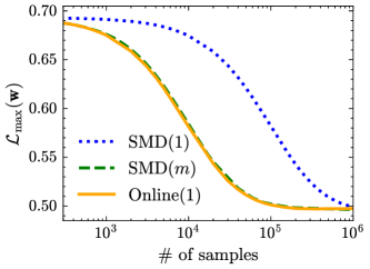
In the experiments, we compare SMD(1) with our algorithms SMD(mm) and Online(11). Fig. 3 plots the maximum risk max(𝐰)\mathcal{L}_{\max}(\mathbf{w}), with respect to the number of iterations. We observe that SMD(mm) is faster than Online(11), which in turn outperforms SMD(11). This observation is consistent with our theories, since their convergence rates are O((logm)/T)O(\sqrt{(\log m)/T}), O(m(logm)/T)O(\sqrt{m(\log m)/T}), and O(m(logm)/T)O(m\sqrt{(\log m)/T}), respectively. Next, we plot max(𝐰)\mathcal{L}_{\max}(\mathbf{w}) against the number of samples consumed by each algorithm in Fig. 3. As can be seen, the curves of SMD(mm) and Online(11) are very close, indicating that they share the same sample complexity, i.e., O(m(logm)/ϵ2)O(m(\log m)/\epsilon^{2}). On the other hand, SMD(11) needs more samples to reach a target precision, which aligns with its higher sample complexity, i.e., O(m2(logm)/ϵ2)O(m^{2}(\log m)/\epsilon^{2}).

Refer to caption
(a) Risk on 𝒫1\mathcal{P}_{1}
Refer to caption
(b) Risk on 𝒫4\mathcal{P}_{4}
Refer to caption
(c) Risk on 𝒫8\mathcal{P}_{8}
Refer to caption
(d) Risk on 𝒫12\mathcal{P}_{12}
Refer to caption
(e) Risk on 𝒫16\mathcal{P}_{16}
Refer to caption
(f) Risk on 𝒫20\mathcal{P}_{20}
Figure 4: Imbalanced settings with the synthetic data set: individual risk versus the number of iterations.

7.3 Weighted GDRO on Imbalanced Data

For experiments on the first synthetic data set, we set the sample size for each group ii as ni=1000×(21i)n_{i}=1000\times(21-i). For those on the Adult data set, we first select 364364 samples randomly from each group, reserving them for later use in estimating the risk of each group. Then, we visit the remaining samples in each group once to simulate the imbalanced setting, where the numbers of samples in 66 groups are 2665626656, 1151911519, 17801780, 17201720, 999999, and 364364. In this way, 𝒫i\mathcal{P}_{i} corresponds to the (unknown) underlying distribution from which the samples in the ii-th group are drawn.

Refer to caption
(a) Risk on 𝒫1\mathcal{P}_{1}
Refer to caption
(b) Risk on 𝒫2\mathcal{P}_{2}
Refer to caption
(c) Risk on 𝒫3\mathcal{P}_{3}
Refer to caption
(d) Risk on 𝒫4\mathcal{P}_{4}
Refer to caption
(e) Risk on 𝒫5\mathcal{P}_{5}
Refer to caption
(f) Risk on 𝒫6\mathcal{P}_{6}
Figure 5: Imbalanced settings with the Adult data set: individual risk versus the number of iterations.

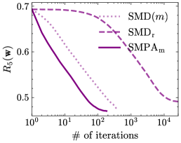
On imbalanced data, we will compare SMDr and SMPAm with the baseline SMD(mm), and examine how the risk on each individual distribution decreases with respect to the number of iterations. Recall that the total number of iterations of SMDr, SMPAm and SMD(mm) are n1n_{1} nm/2n_{m}/2, and nmn_{m}, respectively. We present the experimental results on the synthetic and the Adult data sets in Fig. 4 and Fig. 5, respectively. First, we observe that our SMPAm is faster than both SMDr and SMD(mm) across all distributions, and finally attains the lowest risk in most cases. This behavior aligns with our Theorem 10, which reveals that SMPAm achieves a nearly optimal rate of O((logm)/ni)O((\log m)/\sqrt{n_{i}}) for all distributions 𝒫i\mathcal{P}_{i}, after nm/2n_{m}/2 iterations. We also note that on distribution 𝒫1\mathcal{P}_{1}, the distribution with the most samples, although SMDr converges slowly, its final risk is the lowest, as illustrated in Fig. 4(a) and Fig. 5(a). This phenomenon is again in accordance with our Theorem 9, which shows that the risk of SMDr on 𝒫1\mathcal{P}_{1} reduces at a nearly optimal O((logm)/n1)O(\sqrt{(\log m)/n_{1}}) rate, after n1n_{1} iterations. From Fig. 4(f) and Fig. 5(f), we can see that the final risk of SMD(mm) on the last distribution 𝒫m\mathcal{P}_{m} matches that of SMPAm. This outcome is anticipated, as they exhibit similar convergence rates of O((logm)/nm)O(\sqrt{(\log m)/n_{m}}) and O((logm)/nm)O((\log m)/\sqrt{n_{m}}), respectively.

Refer to caption
(a) k(𝐰)\mathcal{L}_{k}(\mathbf{w}) versus the number of iterations
Refer to caption
(b) k(𝐰)\mathcal{L}_{k}(\mathbf{w}) versus the number of samples
Figure 6: Heterogeneous settings with the synthetic data set.
Refer to caption
(a) Risk on 𝒫1\mathcal{P}_{1}
Refer to caption
(b) Risk on 𝒫2\mathcal{P}_{2}
Refer to caption
(c) Risk on 𝒫5\mathcal{P}_{5}
Refer to caption
(d) Risk on 𝒫10\mathcal{P}_{10}
Refer to caption
(e) Risk on 𝒫15\mathcal{P}_{15}
Refer to caption
(f) Risk on 𝒫20\mathcal{P}_{20}
Figure 7: Heterogeneous settings with the synthetic data set: individual risk versus the number of iterations.

7.4 ATkRO on Heterogeneous Distributions

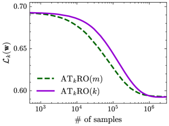
For experiments on heterogeneous distributions, we use the second synthetic data set described in Section 7.1. We first compare our two algorithms ATkRO(mm) and ATkRO(kk), where k=3k=3, and plot the changes of the average top-kk risk k(𝐰)\mathcal{L}_{k}(\mathbf{w}) in Fig. 7. From Theorems 12 and 15, we know that their convergence rates are O((log(m/k))/T)O(\sqrt{(\log(m/k))/T}) and O(m(logm)/(kT))O(\sqrt{m(\log m)/(kT)}), respectively, and their sample complexities are O((mlog(m/k))/ϵ2)O((m\log(m/k))/\epsilon^{2}) and O(m(logm)/ϵ2)O(m(\log m)/\epsilon^{2}), respectively. Fig. 6(a) indicates that ATkRO(mm) indeed converges faster than ATkRO(kk), and Fig. 6(b) shows that ATkRO(mm) requires slightly fewer samples than ATkRO(kk).

Additionally, to demonstrate the advantages of ATkRO, we examine the performance of directly applying the SMD(mm) algorithm, which is designed for GDRO, to the synthetic data set. Fig. 7 presents the changes in risk across a subset of distributions for SMD(mm), ATkRO(mm), and ATkRO(kk). We observe that SMD(mm) concentrates entirely on 𝒫1\mathcal{P}_{1} and achieves the lowest final risk on the outlier distribution 𝒫1\mathcal{P}_{1}, approximately 0.0610.061 lower than ATkRO(mm) and 0.0560.056 lower than ATkRO(kk). However, for the remaining 1919 distributions {𝒫2,,𝒫20}\{\mathcal{P}_{2},\ldots,\mathcal{P}_{20}\}, the risk of SMD(mm) is approximately 0.120.12 higher on average than those of the other two algorithms. Therefore, we conclude that ATkRO can mitigate the impact of the outlier distribution and deliver a more balanced model in heterogeneous distributions compared to GDRO.

7.5 Anytime Capability

To demonstrate the benefits of the anytime capability, we compare SMD(mm) and Online(1) with their anytime extensions SMD(mm)a and Online(1)a on the Adult data set under balanced settings, and ATkRO(mm) and ATkRO(k)(k) with ATkRO(m)a(m)_{\mathrm{a}} and ATkRO(1)a(1)_{\mathrm{a}} on the second synthetic data set, where k=3k=3.

We assign a preset value of T=2000T=2000 for SMD(mm) and Online(1), and T=50000T=50000 for ATkRO(mm) and ATkRO(kk). When the actual number of iterations exceeds the preset number TT, we continue running the four algorithms with the initial parameters. As illustrated in Fig. 8, non-anytime algorithms initially reduce the objective (the maximum risk or the average top-kk risk) more rapidly than anytime algorithms before reaching the predetermined TT, where they achieve minimal values. However, as the number of iterations increases, their curves plateau or even increase due to sub-optimal parameters. In contrast, the anytime extensions, with time-varying step sizes, consistently reduce their targets over time, eventually falling below the risk attained by the corresponding non-anytime algorithms.

Refer to caption
Refer to caption
(a) The Adult data set
Refer to caption
Refer to caption
(b) The synthetic data set
Figure 8: The performance of different methods versus the number of iterations. Blue dashed lines indicate the predetermined TT for non-anytime algorithms.

8 Conclusion

For the GDRO problem, we develop two SA approaches based on SMD and non-oblivious MAB, which consume mm and 11 sample per round, respectively, and both achieve a nearly optimal sample complexity of O(m(logm)/ϵ2)O(m(\log m)/\epsilon^{2}). Then, we consider two special scenarios: imbalanced data and heterogeneous distributions. In the first scenario, we formulate a weighted GDRO problem and propose two methods by incorporating non-uniform sampling into SMD and using mini-batches with SMPA, respectively. These methods yield distribution-dependent convergence rates, and in particular, the latter one attains nearly optimal rates for multiple distributions simultaneously. In the second scenario, we formulate an ATkRO problem and propose two algorithms: one using SMD with mm samples per round, obtaining an O(m(log(m/k))/ϵ2)O(m(\log(m/k))/\epsilon^{2}) sample complexity, and the other combining SMD with non-oblivious combinatorial semi-bandits, using kk samples per round and achieving an O(m(logm)/ϵ2)O(m(\log m)/\epsilon^{2}) sample complexity. For both GDRO and ATkRO, we have also developed SA algorithms with anytime capabilities.

Appendix A Supporting Lemmas

A.1 Proof of Lemma 11

We first define 𝐪^\hat{\mathbf{q}} as

νq(𝐪^)=νq(𝐪0)η𝐠.\nabla\nu_{q}\left(\hat{\mathbf{q}}\right)=\nabla\nu_{q}(\mathbf{q}_{0})-\eta\mathbf{g}. (138)

Then, we have

argmin𝐪SSm,kBq(𝐪,𝐪^)=argmin𝐪SSm,k{νq(𝐪)νq(𝐪^)νq(𝐪^),𝐪𝐪^}\displaystyle\operatorname*{argmin}_{\mathbf{q}\in\SS_{m,k}}B_{q}(\mathbf{q},\hat{\mathbf{q}})=\operatorname*{argmin}_{\mathbf{q}\in\SS_{m,k}}\big{\{}\nu_{q}(\mathbf{q})-\nu_{q}\left(\hat{\mathbf{q}}\right)-\langle\nabla\nu_{q}\left(\hat{\mathbf{q}}\right),\mathbf{q}-\hat{\mathbf{q}}\rangle\big{\}}
=\displaystyle= argmin𝐪SSm,k{νq(𝐪)νq(𝐪^),𝐪}=(138)argmin𝐪SSm,k{νq(𝐪)νq(𝐪0)η𝐠,𝐪}\displaystyle\operatorname*{argmin}_{\mathbf{q}\in\SS_{m,k}}\big{\{}\nu_{q}(\mathbf{q})-\langle\nabla\nu_{q}\left(\hat{\mathbf{q}}\right),\mathbf{q}\rangle\big{\}}\overset{\eqref{q_OMD_1}}{=}\operatorname*{argmin}_{\mathbf{q}\in\SS_{m,k}}\big{\{}\nu_{q}(\mathbf{q})-\langle\nabla\nu_{q}(\mathbf{q}_{0})-\eta\mathbf{g},\mathbf{q}\rangle\big{\}}
=\displaystyle= argmin𝐪SSm,k{η𝐠,𝐪𝐪0+Bc(𝐪,𝐪0)}=(50).\displaystyle\operatorname*{argmin}_{\mathbf{q}\in\SS_{m,k}}\big{\{}\eta\langle\mathbf{g},\mathbf{q}-\mathbf{q}_{0}\rangle+B_{c}(\mathbf{q},\mathbf{q}_{0})\big{\}}=\eqref{q_OMD_0}.

Recall that Bq(,)B_{q}(\cdot,\cdot) is defined in terms of the neg-entropy, i.e., νq(𝐪)=i=1mqilnqi\nu_{q}(\mathbf{q})=\sum_{i=1}^{m}q_{i}\ln q_{i}, we have [νq(𝐪)]i=1+lnqi[\nabla\nu_{q}(\mathbf{q})]_{i}=1+\ln q_{i}. Therefore, the ii-th component of 𝐪^\hat{\mathbf{q}} can be computed as

q^i=exp([νq(𝐪0)]iηgi1)=exp(lnq0,iηgi)=q0,ieηgi.\hat{q}_{i}=\exp\big{(}[\nabla\nu_{q}(\mathbf{q}_{0})]_{i}-\eta g_{i}-1\big{)}=\exp\left(\ln q_{0,i}-\eta g_{i}\right)=q_{0,i}e^{-\eta g_{i}}.

A.2 Proof of Lemma 18

The proof follows the argument of Neu (2015, Proof of Lemma 1), and we generalize it to the setting with stochastic rewards. First, observe that for any i[m]i\in[m] and t[T]t\in[T],

ξ~t,i=\displaystyle\tilde{\xi}_{t,i}={} ξ^t,ipt,i+γt𝕀[it=i]\displaystyle\frac{\hat{\xi}_{t,i}}{p_{t,i}+\gamma_{t}}\cdot\mathbb{I}[i_{t}=i]
\displaystyle\leq{} ξ^t,ipt,i+γtξ^t,i𝕀[it=i]\displaystyle\frac{\hat{\xi}_{t,i}}{p_{t,i}+\gamma_{t}\hat{\xi}_{t,i}}\cdot\mathbb{I}[i_{t}=i] (ξ^t,i[0,1]\hat{\xi}_{t,i}\in[0,1])
=\displaystyle={} 12γt2γtξ^t,i/pt,i1+γtξ^t,i/pt,i𝕀[it=i]\displaystyle\frac{1}{2\gamma_{t}}\frac{2\gamma_{t}\cdot\hat{\xi}_{t,i}/p_{t,i}}{1+\gamma_{t}\cdot\hat{\xi}_{t,i}/p_{t,i}}\cdot\mathbb{I}[i_{t}=i]
\displaystyle\leq{} 1βtlog(1+βtξ¯t,i)\displaystyle\frac{1}{\beta_{t}}\log\left(1+\beta_{t}\bar{\xi}_{t,i}\right) (139)

where the last step is due to the inequality z1+z/2log(1+z)\frac{z}{1+z/2}\leq\log(1+z) for z0z\geq 0 and we introduce the notations βt=2γt\beta_{t}=2\gamma_{t} and ξ¯t,i=(ξ^t,i/pt,i)𝕀[it=i]\bar{\xi}_{t,i}=(\hat{\xi}_{t,i}/p_{t,i})\cdot\mathbb{I}[i_{t}=i] to simplify the presentation.

Define the notation λ~t=i=1mαt,iξ~t,i\tilde{\lambda}_{t}=\sum_{i=1}^{m}\alpha_{t,i}\tilde{\xi}_{t,i} and λt=i=1mαt,iξt,i\lambda_{t}=\sum_{i=1}^{m}\alpha_{t,i}\xi_{t,i}. Then, we have

Et1[exp(λ~t)]=\displaystyle\mathrm{E}_{t-1}\left[\exp(\tilde{\lambda}_{t})\right]={} Et1[exp(i=1mαt,iξ~t,i)]\displaystyle\mathrm{E}_{t-1}\left[\exp\Big{(}\sum_{i=1}^{m}\alpha_{t,i}\tilde{\xi}_{t,i}\Big{)}\right]
(139)\displaystyle\overset{\eqref{eq:concentration-1}}{\leq}{} Et1[exp(i=1mαt,iβtlog(1+βtξ¯t,i))]\displaystyle\mathrm{E}_{t-1}\left[\exp\left(\sum_{i=1}^{m}\frac{\alpha_{t,i}}{\beta_{t}}\log\Big{(}1+\beta_{t}\bar{\xi}_{t,i}\Big{)}\right)\right]
\displaystyle\leq{} Et1[exp(i=1mlog(1+αt,iξ¯t,i))]\displaystyle\mathrm{E}_{t-1}\left[\exp\left(\sum_{i=1}^{m}\log\Big{(}1+\alpha_{t,i}\bar{\xi}_{t,i}\Big{)}\right)\right] (αt,iβt1\frac{\alpha_{t,i}}{\beta_{t}}\leq 1 by assumption)
=\displaystyle={} Et1[Πi=1m(1+αt,iξ¯t,i)]=Et1[1+i=1mαt,iξ¯t,i]\displaystyle\mathrm{E}_{t-1}\left[\Pi_{i=1}^{m}\big{(}1+\alpha_{t,i}\bar{\xi}_{t,i}\big{)}\right]=\mathrm{E}_{t-1}\left[1+\sum_{i=1}^{m}\alpha_{t,i}\bar{\xi}_{t,i}\right]
=\displaystyle={} 1+i=1mαt,iξt,iexp(i=1mαt,iξt,i)=exp(λt)\displaystyle 1+\sum_{i=1}^{m}\alpha_{t,i}\xi_{t,i}\leq\exp\left(\sum_{i=1}^{m}\alpha_{t,i}\xi_{t,i}\right)=\exp(\lambda_{t}) (140)

where the second inequality is by the inequality xlog(1+y)log(1+xy)x\log(1+y)\leq\log(1+xy) that holds for all y1y\geq-1 and x[0,1]x\in[0,1], the equality Et1[Πi=1m(1+αt,iξ¯t,i)]=Et1[1+i=1mαt,iξ¯t,i]\mathrm{E}_{t-1}\left[\Pi_{i=1}^{m}\big{(}1+\alpha_{t,i}\bar{\xi}_{t,i}\big{)}\right]=\mathrm{E}_{t-1}\left[1+\sum_{i=1}^{m}\alpha_{t,i}\bar{\xi}_{t,i}\right] follows from the fact that ξ¯t,iξ¯t,j=0\bar{\xi}_{t,i}\cdot\bar{\xi}_{t,j}=0 holds whenever iji\neq j, and the last line is due to Et1[ξ¯t,i]=Et1[(ξ^t,i/pt,i)𝕀[it=i]]=ξt,i\mathrm{E}_{t-1}[\bar{\xi}_{t,i}]=\mathrm{E}_{t-1}[(\hat{\xi}_{t,i}/p_{t,i})\cdot\mathbb{I}[i_{t}=i]]=\xi_{t,i} and the inequality 1+zez1+z\leq e^{z} for all zz\in\mathbb{R}.

As a result, from (140) we conclude that the process Zt=exp(s=1t(λ~sλs))Z_{t}=\exp\big{(}\sum_{s=1}^{t}(\tilde{\lambda}_{s}-\lambda_{s})\big{)} is a supermartingale. Indeed, Et1[Zt]=Et1[exp(s=1t1(λ~sλs))exp(λ~tλt)]Zt1\mathrm{E}_{t-1}[Z_{t}]=\mathrm{E}_{t-1}\big{[}\exp\big{(}\sum_{s=1}^{t-1}(\tilde{\lambda}_{s}-\lambda_{s})\big{)}\cdot\exp(\tilde{\lambda}_{t}-\lambda_{t})\big{]}\leq Z_{t-1}. Thus, we have E[ZT]E[ZT1E[Z0]=1\mathrm{E}[Z_{T}]\leq\mathrm{E}[Z_{T-1}\leq\ldots\leq\mathrm{E}[Z_{0}]=1. By Markov’s inequality,

Pr[t=1T(λ~tλt)>ϵ]E[exp(t=1T(λ~tλt))]exp(ϵ)exp(ϵ)\Pr\left[\sum_{t=1}^{T}(\tilde{\lambda}_{t}-\lambda_{t})>\epsilon\right]\leq\mathrm{E}\left[\exp\left(\sum_{t=1}^{T}(\tilde{\lambda}_{t}-\lambda_{t})\right)\right]\cdot\exp(-\epsilon)\leq\exp(-\epsilon)

holds for any ϵ>0\epsilon>0. By setting exp(ϵ)=δ\exp(-\epsilon)=\delta and solving the value, we complete the proof for (87). And the inequality (88) for the scenario γt=γ\gamma_{t}=\gamma can be immediately obtained by setting αt,i=2γ𝕀[i=j]\alpha_{t,i}=2\gamma\cdot\mathbb{I}[i=j] and taking the union bound over all j[m]j\in[m].

A.3 Proof of Lemma 20

From the definition of norms in (61), we have

F([𝐰;𝐪])F([𝐰;𝐪])2=[i=1mqipiRi(𝐰)i=1mqipiRi(𝐰);[p1R1(𝐰)p1R1(𝐰),,pmRm(𝐰)pmRm(𝐰)]]2=2D2i=1mqipiRi(𝐰)i=1mqipiRi(𝐰)w,2+2[p1R1(𝐰)p1R1(𝐰),,pmRm(𝐰)pmRm(𝐰)]2lnm=2D2i=1mqipiRi(𝐰)i=1mqipiRi(𝐰)+i=1mqipiRi(𝐰)i=1mqipiRi(𝐰)w,2+2[p1R1(𝐰)p1R1(𝐰),,pmRm(𝐰)pmRm(𝐰)]2lnm4D2i=1mqipiRi(𝐰)i=1mqipiRi(𝐰)w,2:=A+4D2i=1mqipiRi(𝐰)i=1mqipiRi(𝐰)w,2:=B+2maxi[m]|pi[Ri(𝐰)Ri(𝐰)]|2lnm:=C.\begin{split}&\|F([\mathbf{w};\mathbf{q}])-F([\mathbf{w}^{\prime};\mathbf{q}^{\prime}])\|_{*}^{2}\\ =&\left\|\left[\sum_{i=1}^{m}q_{i}p_{i}\nabla R_{i}(\mathbf{w})-\sum_{i=1}^{m}q_{i}^{\prime}p_{i}\nabla R_{i}(\mathbf{w}^{\prime});\right.\right.\\ &\left.\left.\big{[}p_{1}R_{1}(\mathbf{w}^{\prime})-p_{1}R_{1}(\mathbf{w}),\ldots,p_{m}R_{m}(\mathbf{w}^{\prime})-p_{m}R_{m}(\mathbf{w})\big{]}^{\top}\right]\right\|_{*}^{2}\\ =&2D^{2}\left\|\sum_{i=1}^{m}q_{i}p_{i}\nabla R_{i}(\mathbf{w})-\sum_{i=1}^{m}q_{i}^{\prime}p_{i}\nabla R_{i}(\mathbf{w}^{\prime})\right\|_{w,*}^{2}\\ &+2\left\|\big{[}p_{1}R_{1}(\mathbf{w}^{\prime})-p_{1}R_{1}(\mathbf{w}),\ldots,p_{m}R_{m}(\mathbf{w}^{\prime})-p_{m}R_{m}(\mathbf{w})\big{]}^{\top}\right\|_{\infty}^{2}\ln m\\ =&2D^{2}\left\|\sum_{i=1}^{m}q_{i}p_{i}\nabla R_{i}(\mathbf{w})-\sum_{i=1}^{m}q_{i}^{\prime}p_{i}\nabla R_{i}(\mathbf{w})+\sum_{i=1}^{m}q_{i}^{\prime}p_{i}\nabla R_{i}(\mathbf{w})-\sum_{i=1}^{m}q_{i}^{\prime}p_{i}\nabla R_{i}(\mathbf{w}^{\prime})\right\|_{w,*}^{2}\\ &+2\left\|\big{[}p_{1}R_{1}(\mathbf{w}^{\prime})-p_{1}R_{1}(\mathbf{w}),\ldots,p_{m}R_{m}(\mathbf{w}^{\prime})-p_{m}R_{m}(\mathbf{w})\big{]}^{\top}\right\|_{\infty}^{2}\ln m\\ \leq&\underbrace{4D^{2}\left\|\sum_{i=1}^{m}q_{i}p_{i}\nabla R_{i}(\mathbf{w})-\sum_{i=1}^{m}q_{i}^{\prime}p_{i}\nabla R_{i}(\mathbf{w})\right\|_{w,*}^{2}}_{:=A}\\ &+\underbrace{4D^{2}\left\|\sum_{i=1}^{m}q_{i}^{\prime}p_{i}\nabla R_{i}(\mathbf{w})-\sum_{i=1}^{m}q_{i}^{\prime}p_{i}\nabla R_{i}(\mathbf{w}^{\prime})\right\|_{w,*}^{2}}_{:=B}+\underbrace{2\max_{i\in[m]}\left|p_{i}\big{[}R_{i}(\mathbf{w})-R_{i}(\mathbf{w}^{\prime})\big{]}\right|^{2}\ln m}_{:=C}.\end{split}

To bound term AA, we have

4D2i=1mqipiRi(𝐰)i=1mqipiRi(𝐰)w,24D2(i=1m|qiqi|piRi(𝐰)w,)2(114)4D2(i=1m|qiqi|piG)24D2G2pmax2𝐪𝐪12.\begin{split}&4D^{2}\left\|\sum_{i=1}^{m}q_{i}p_{i}\nabla R_{i}(\mathbf{w})-\sum_{i=1}^{m}q_{i}^{\prime}p_{i}\nabla R_{i}(\mathbf{w})\right\|_{w,*}^{2}\\ \leq&4D^{2}\left(\sum_{i=1}^{m}|q_{i}-q_{i}^{\prime}|\|p_{i}\nabla R_{i}(\mathbf{w})\|_{w,*}\right)^{2}\overset{\text{(\ref{eqn:R:Lipschitz:1})}}{\leq}4D^{2}\left(\sum_{i=1}^{m}|q_{i}-q_{i}^{\prime}|p_{i}G\right)^{2}\leq 4D^{2}G^{2}p_{\max}^{2}\|\mathbf{q}-\mathbf{q}^{\prime}\|_{1}^{2}.\end{split}

where pmaxp_{\max} is defined in (44). To bound BB, we have

4D2i=1mqipiRi(𝐰)i=1mqipiRi(𝐰)w,24D2(i=1mqipiRi(𝐰)Ri(𝐰)w,)2(43)4D2(i=1mqipiL𝐰𝐰w)24D2L2pmax2𝐰𝐰w2(i=1mqi)2=4D2L2pmax2𝐰𝐰w2.\begin{split}&4D^{2}\left\|\sum_{i=1}^{m}q_{i}^{\prime}p_{i}\nabla R_{i}(\mathbf{w})-\sum_{i=1}^{m}q_{i}^{\prime}p_{i}\nabla R_{i}(\mathbf{w}^{\prime})\right\|_{w,*}^{2}\\ \leq&4D^{2}\left(\sum_{i=1}^{m}q_{i}^{\prime}p_{i}\left\|\nabla R_{i}(\mathbf{w})-\nabla R_{i}(\mathbf{w}^{\prime})\right\|_{w,*}\right)^{2}\overset{\text{(\ref{eqn:smooth:R})}}{\leq}4D^{2}\left(\sum_{i=1}^{m}q_{i}^{\prime}p_{i}L\|\mathbf{w}-\mathbf{w}^{\prime}\|_{w}\right)^{2}\\ \leq&4D^{2}L^{2}p_{\max}^{2}\|\mathbf{w}-\mathbf{w}^{\prime}\|_{w}^{2}\left(\sum_{i=1}^{m}q_{i}^{\prime}\right)^{2}=4D^{2}L^{2}p_{\max}^{2}\|\mathbf{w}-\mathbf{w}^{\prime}\|_{w}^{2}.\end{split}

To bound CC, we have

2maxi[m]|pi[Ri(𝐰)Ri(𝐰)]|2lnm(115)2maxi[m]|piG𝐰𝐰w|2lnm2G2pmax2𝐰𝐰w2lnm.\begin{split}&2\max_{i\in[m]}\left|p_{i}\big{[}R_{i}(\mathbf{w})-R_{i}(\mathbf{w}^{\prime})\big{]}\right|^{2}\ln m\\ \overset{\text{(\ref{eqn:R:Lipschitz:2})}}{\leq}&2\max_{i\in[m]}\left|p_{i}G\|\mathbf{w}-\mathbf{w}^{\prime}\|_{w}\right|^{2}\ln m\leq 2G^{2}p_{\max}^{2}\|\mathbf{w}-\mathbf{w}^{\prime}\|_{w}^{2}\ln m.\end{split}

Putting everything together, we have

F([𝐰;𝐪])F([𝐰;𝐪])2(4D2L2+2G2lnm)pmax2𝐰𝐰w2+4D2G2pmax2𝐪𝐪12pmax2(8D4L2+8D2G2lnm)(12D2𝐰𝐰w2+12lnm𝐪𝐪12)=pmax2(8D4L2+8D2G2lnm)[𝐰𝐰;𝐪𝐪]2\begin{split}&\|F([\mathbf{w};\mathbf{q}])-F([\mathbf{w}^{\prime};\mathbf{q}^{\prime}])\|_{*}^{2}\leq(4D^{2}L^{2}+2G^{2}\ln m)p_{\max}^{2}\|\mathbf{w}-\mathbf{w}^{\prime}\|_{w}^{2}+4D^{2}G^{2}p_{\max}^{2}\|\mathbf{q}-\mathbf{q}^{\prime}\|_{1}^{2}\\ \leq&p_{\max}^{2}(8D^{4}L^{2}+8D^{2}G^{2}\ln m)\left(\frac{1}{2D^{2}}\|\mathbf{w}-\mathbf{w}^{\prime}\|_{w}^{2}+\frac{1}{2\ln m}\|\mathbf{q}-\mathbf{q}^{\prime}\|_{1}^{2}\right)\\ =&p_{\max}^{2}(8D^{4}L^{2}+8D^{2}G^{2}\ln m)\big{\|}[\mathbf{w}-\mathbf{w}^{\prime};\mathbf{q}-\mathbf{q}^{\prime}]\big{\|}^{2}\end{split}

which implies

F([𝐰;𝐪])F([𝐰;𝐪])pmax8D4L2+8D2G2lnm[𝐰𝐰;𝐪𝐪]L~[𝐰𝐰;𝐪𝐪]\begin{split}\|F([\mathbf{w};\mathbf{q}])-F([\mathbf{w}^{\prime};\mathbf{q}^{\prime}])\|_{*}\leq&p_{\max}\sqrt{8D^{4}L^{2}+8D^{2}G^{2}\ln m}\big{\|}[\mathbf{w}-\mathbf{w}^{\prime};\mathbf{q}-\mathbf{q}^{\prime}]\big{\|}\\ \leq&\widetilde{L}\big{\|}[\mathbf{w}-\mathbf{w}^{\prime};\mathbf{q}-\mathbf{q}^{\prime}]\big{\|}\end{split}

where L~\widetilde{L} is defined in (44).

A.4 Proof of Lemma 21

The light tail condition, required by Juditsky et al. (2011), is essentially the sub-Gaussian condition. To this end, we introduce the following sub-gaussian properties (Vershynin, 2018, Proposition 2.5.2).

Proposition 1 (Sub-gaussian properties)

Let XX be a random variable. Then the following properties are equivalent; the parameters Ki>0K_{i}>0 appearing in these properties differ from each other by at most an absolute constant factor.

  1. (i)

    The tails of XX satisfy

    Pr[|X|t]2exp(t2/K12),t0.\Pr[|X|\geq t]\leq 2\exp(-t^{2}/K_{1}^{2}),\ \forall t\geq 0.
  2. (ii)

    The moments of XX satisfy

    XLp=(E|X|p)1/pK2p,p1.\|X\|_{L_{p}}=\left(\mathrm{E}|X|^{p}\right)^{1/p}\leq K_{2}\sqrt{p},\ \forall p\geq 1.
  3. (iii)

    The moment generating function (MGF) of X2X^{2} satisfies

    E[exp(λ2X2)]exp(K32λ2),λ such that |λ|1/K3.\mathrm{E}\big{[}\exp(\lambda^{2}X^{2})\big{]}\leq\exp(K_{3}^{2}\lambda^{2}),\ \forall\lambda\textrm{ such that }|\lambda|\leq 1/K_{3}.
  4. (iv)

    The MGF of X2X^{2} is bounded at some point, namely

    E[exp(X2/K42)]2.\mathrm{E}\big{[}\exp(X^{2}/K_{4}^{2})\big{]}\leq 2.

From the above proposition, we observe that the exact value of those constant K1,,K5K_{1},\ldots,K_{5} is not important, and it is very tedious to calculate them. So, in the following, we only focus on the order of those constants. To simplify presentations, we use cc to denote an absolute constant that is independent of all the essential parameters, and its value may change from line to line.

Since

F([𝐰;𝐪])𝐠([𝐰;𝐪])2=2D2𝐰φ(𝐰,𝐪)𝐠w(𝐰,𝐪)w,2+2𝐪φ(𝐰,𝐪)𝐠q(𝐰,𝐪)2lnm,\begin{split}&\|F([\mathbf{w};\mathbf{q}])-\mathbf{g}([\mathbf{w};\mathbf{q}])\|_{*}^{2}\\ =&2D^{2}\|\nabla_{\mathbf{w}}\varphi(\mathbf{w},\mathbf{q})-\mathbf{g}_{w}(\mathbf{w},\mathbf{q})\|_{w,*}^{2}+2\|\nabla_{\mathbf{q}}\varphi(\mathbf{w},\mathbf{q})-\mathbf{g}_{q}(\mathbf{w},\mathbf{q})\|_{\infty}^{2}\ln m,\end{split}

we proceed to analyze the behavior of 𝐰φ(𝐰,𝐪)𝐠w(𝐰,𝐪)w,2\|\nabla_{\mathbf{w}}\varphi(\mathbf{w},\mathbf{q})-\mathbf{g}_{w}(\mathbf{w},\mathbf{q})\|_{w,*}^{2} and 𝐪φ(𝐰,𝐪)𝐠q(𝐰,𝐪)2\|\nabla_{\mathbf{q}}\varphi(\mathbf{w},\mathbf{q})-\mathbf{g}_{q}(\mathbf{w},\mathbf{q})\|_{\infty}^{2}. To this end, we have the following lemma.

Lemma 24

We have

E[exp(1cκG2ωmax𝐰φ(𝐰,𝐪)𝐠w(𝐰,𝐪)w,2)]2,E[exp(1cωmaxlnm𝐪φ(𝐰,𝐪)𝐠q(𝐰,𝐪)2)]2\begin{split}&\mathrm{E}\bigg{[}\exp\left(\frac{1}{c\kappa G^{2}\omega_{\max}}\|\nabla_{\mathbf{w}}\varphi(\mathbf{w},\mathbf{q})-\mathbf{g}_{w}(\mathbf{w},\mathbf{q})\|_{w,*}^{2}\right)\bigg{]}\leq 2,\\ &\mathrm{E}\left[\exp\left(\frac{1}{c\omega_{\max}\ln m}\|\nabla_{\mathbf{q}}\varphi(\mathbf{w},\mathbf{q})-\mathbf{g}_{q}(\mathbf{w},\mathbf{q})\|_{\infty}^{2}\right)\right]\leq 2\end{split} (141)

where ωmax\omega_{\max} is defined in (44) and c>0c>0 is an absolute constant.

From Lemma 24, we have

E[exp(12cκD2G2ωmax+2cωmaxln2mF([𝐰;𝐪])𝐠([𝐰,𝐪])2)]=E[exp(2D22cκD2G2ωmax+2cωmaxln2m𝐰φ(𝐰,𝐪)𝐠w(𝐰,𝐪)w,2+2lnm2cκD2G2ωmax+2cωmaxln2m𝐪φ(𝐰,𝐪)𝐠q(𝐰,𝐪)2)]=E[exp(κD2G2κD2G2+ln2m𝐰φ(𝐰,𝐪)𝐠w(𝐰,𝐪)w,2cκG2ωmax+ln2mκD2G2+ln2m𝐪φ(𝐰,𝐪)𝐠q(𝐰,𝐪)2cωmaxlnm)]\begin{split}&\mathrm{E}\left[\exp\left(\frac{1}{2c\kappa D^{2}G^{2}\omega_{\max}+2c\omega_{\max}\ln^{2}m}\|F([\mathbf{w};\mathbf{q}])-\mathbf{g}([\mathbf{w},\mathbf{q}])\|_{*}^{2}\right)\right]\\ =&\mathrm{E}\left[\exp\left(\frac{2D^{2}}{2c\kappa D^{2}G^{2}\omega_{\max}+2c\omega_{\max}\ln^{2}m}\|\nabla_{\mathbf{w}}\varphi(\mathbf{w},\mathbf{q})-\mathbf{g}_{w}(\mathbf{w},\mathbf{q})\|_{w,*}^{2}\right.\right.\\ &\left.\left.+\frac{2\ln m}{2c\kappa D^{2}G^{2}\omega_{\max}+2c\omega_{\max}\ln^{2}m}\|\nabla_{\mathbf{q}}\varphi(\mathbf{w},\mathbf{q})-\mathbf{g}_{q}(\mathbf{w},\mathbf{q})\|_{\infty}^{2}\right)\right]\\ =&\mathrm{E}\left[\exp\left(\frac{\kappa D^{2}G^{2}}{\kappa D^{2}G^{2}+\ln^{2}m}\frac{\|\nabla_{\mathbf{w}}\varphi(\mathbf{w},\mathbf{q})-\mathbf{g}_{w}(\mathbf{w},\mathbf{q})\|_{w,*}^{2}}{c\kappa G^{2}\omega_{\max}}\right.\right.\\ &\left.\left.+\frac{\ln^{2}m}{\kappa D^{2}G^{2}+\ln^{2}m}\frac{\|\nabla_{\mathbf{q}}\varphi(\mathbf{w},\mathbf{q})-\mathbf{g}_{q}(\mathbf{w},\mathbf{q})\|_{\infty}^{2}}{c\omega_{\max}\ln m}\right)\right]\\ \end{split}
κD2G2κD2G2+ln2mE[exp(𝐰φ(𝐰,𝐪)𝐠w(𝐰,𝐪)w,2cκG2ωmax)]+ln2mκD2G2+ln2mE[exp(𝐪φ(𝐰,𝐪)𝐠q(𝐰,𝐪)2cωmaxlnm)](141)κD2G2κD2G2+ln2m2+ln2mκD2G2+ln2m2=2\begin{split}\leq&\frac{\kappa D^{2}G^{2}}{\kappa D^{2}G^{2}+\ln^{2}m}\mathrm{E}\left[\exp\left(\frac{\|\nabla_{\mathbf{w}}\varphi(\mathbf{w},\mathbf{q})-\mathbf{g}_{w}(\mathbf{w},\mathbf{q})\|_{w,*}^{2}}{c\kappa G^{2}\omega_{\max}}\right)\right]\\ &+\frac{\ln^{2}m}{\kappa D^{2}G^{2}+\ln^{2}m}\mathrm{E}\left[\exp\left(\frac{\|\nabla_{\mathbf{q}}\varphi(\mathbf{w},\mathbf{q})-\mathbf{g}_{q}(\mathbf{w},\mathbf{q})\|_{\infty}^{2}}{c\omega_{\max}\ln m}\right)\right]\\ \overset{\text{(\ref{eqn:variance:two:norm})}}{\leq}&\frac{\kappa D^{2}G^{2}}{\kappa D^{2}G^{2}+\ln^{2}m}2+\frac{\ln^{2}m}{\kappa D^{2}G^{2}+\ln^{2}m}2=2\end{split}

where the first inequality follows from Jensen’s inequality.

A.5 Proof of Lemma 22

The proof is built upon that of Corollary 1 of Neu (2015). Let β=2γ\beta=2\gamma and ξt,i=ξ^t,ikpt,i𝕀[it]\xi_{t,i}^{\prime}=\frac{\hat{\xi}_{t,i}}{kp_{t,i}}\mathbb{I}[i\in\mathcal{I}_{t}]. First, we have

ξ~t,i=ξ^t,ikpt,i+γ𝕀[it]ξ^t,ikpt,i+γξ^t,i𝕀[it]=12γ2γξ^t,i/kpt,i1+γξ^t,i/kpt,i𝕀[it]1βlog(1+βξt,i)\begin{split}\tilde{\xi}_{t,i}=&\frac{\hat{\xi}_{t,i}}{kp_{t,i}+\gamma}\mathbb{I}[i\in\mathcal{I}_{t}]\\ \leq&\frac{\hat{\xi}_{t,i}}{kp_{t,i}+\gamma\hat{\xi}_{t,i}}\mathbb{I}[i\in\mathcal{I}_{t}]=\frac{1}{2\gamma}\cdot\frac{2\gamma\hat{\xi}_{t,i}/kp_{t,i}}{1+\gamma\hat{\xi}_{t,i}/kp_{t,i}}\mathbb{I}[i\in\mathcal{I}_{t}]\leq\frac{1}{\beta}\cdot\log\left(1+\beta\xi_{t,i}^{\prime}\right)\end{split} (142)

where the first inequality follows from ξ^t,i[0,1]\hat{\xi}_{t,i}\in[0,1] and last inequality from the elementary inequality z1+z/2\frac{z}{1+z/2}\leq log(1+z)\log(1+z) that holds for all z0z\geq 0. Second, from the property of DepRound, we have

Et1[ξt,i]=Et1[ξt,ikpt,i𝕀[it]]=(53)ξt,i.\mathrm{E}_{t-1}[\xi_{t,i}^{\prime}]=\mathrm{E}_{t-1}\left[\frac{\xi_{t,i}}{kp_{t,i}}\mathbb{I}[i\in\mathcal{I}_{t}]\right]\overset{\text{(\ref{DepRound:prop})}}{=}\xi_{t,i}. (143)

Then, we have

Et1[exp(βξ~t,i)](142)Et1[1+βξt,i]=(143)1+βξt,iexp(βξt,i).\mathrm{E}_{t-1}\left[\exp(\beta\tilde{\xi}_{t,i})\right]\overset{\text{(\ref{eqn:cor1:1})}}{\leq}\mathrm{E}_{t-1}\left[1+\beta\xi_{t,i}^{\prime}\right]\overset{\text{(\ref{eqn:cor1:2})}}{=}1+\beta\xi_{t,i}\leq\exp(\beta\xi_{t,i}).

Then, by repeating the subsequent analysis from Corollary 1 of Neu (2015), we can derive this lemma.

A.6 Proof of Lemma 24

To analyze 𝐰φ(𝐰,𝐪)𝐠w(𝐰,𝐪)w,2\|\nabla_{\mathbf{w}}\varphi(\mathbf{w},\mathbf{q})-\mathbf{g}_{w}(\mathbf{w},\mathbf{q})\|_{w,*}^{2}, we first consider the approximation error caused by samples from 𝒫i\mathcal{P}_{i}:

nmnij=1ni/nm(𝐰;𝐳(i,j))Ri(𝐰)w,=nmnij=1ni/nm[(𝐰;𝐳(i,j))Ri(𝐰)]w,.\left\|\frac{n_{m}}{n_{i}}\sum_{j=1}^{n_{i}/n_{m}}\nabla\ell(\mathbf{w};\mathbf{z}^{(i,j)})-\nabla R_{i}(\mathbf{w})\right\|_{w,*}=\left\|\frac{n_{m}}{n_{i}}\sum_{j=1}^{n_{i}/n_{m}}\left[\nabla\ell(\mathbf{w};\mathbf{z}^{(i,j)})-\nabla R_{i}(\mathbf{w})\right]\right\|_{w,*}.

Under the regularity condition of w,\|\cdot\|_{w,*} in Assumption 6, we have, for any γ0\gamma\geq 0,

nmnij=1ni/nm[(𝐰;𝐳(i,j))Ri(𝐰)]w,2G(2κ+2γ)nmniexp(γ2/2)\left\|\frac{n_{m}}{n_{i}}\sum_{j=1}^{n_{i}/n_{m}}\left[\nabla\ell(\mathbf{w};\mathbf{z}^{(i,j)})-\nabla R_{i}(\mathbf{w})\right]\right\|_{w,*}\geq 2G(\sqrt{2\kappa}+\sqrt{2}\gamma)\sqrt{\frac{n_{m}}{n_{i}}}\leq\exp(-\gamma^{2}/2) (144)

which is a directly consequence of the concentration inequality of vector norms (Juditsky and Nemirovski, 2008, Theorem 2.1.(iii)) and (116). Then, we introduce the following lemma to simplify (144).

Lemma 25

Suppose we have

Pr[Xα+γ]exp(γ2/2),γ>0\Pr\left[X\geq\alpha+\gamma\right]\leq\exp({-}\gamma^{2}/2),\ \forall\gamma>0

where XX is nonnegative. Then, we have

Pr[Xγ]2exp(γ2/max(6α2,8)),γ>0.\Pr\left[X\geq\gamma\right]\leq 2\exp\big{(}{-}\gamma^{2}/\max(6\alpha^{2},8)\big{)},\ \forall\gamma>0.

From (144) and Lemma 25, we have

Pr[122Gninmnmnij=1ni/nm[(𝐰;𝐳(i,j))Ri(𝐰)]w,γ]2exp(γ2/max(6κ,8))2exp(γ2/(8κ)),γ>0\begin{split}&\Pr\left[\frac{1}{2\sqrt{2}G}\sqrt{\frac{n_{i}}{n_{m}}}\left\|\frac{n_{m}}{n_{i}}\sum_{j=1}^{n_{i}/n_{m}}\left[\nabla\ell(\mathbf{w};\mathbf{z}^{(i,j)})-\nabla R_{i}(\mathbf{w})\right]\right\|_{w,*}\geq\gamma\right]\\ \leq&2\exp\big{(}{-}\gamma^{2}/\max(6\kappa,8)\big{)}\leq 2\exp\big{(}{-}\gamma^{2}/(8\kappa)\big{)},\ \forall\gamma>0\end{split}

which satisfies the Proposition 1.(i). From the equivalence between Proposition 1.(i) and Proposition 1.(iv), we have

E[exp(nmnij=1ni/nm[(𝐰;𝐳(i,j))Ri(𝐰)]w,2/cκG2nmni)]2.\mathrm{E}\left[\exp\left(\left.\left\|\frac{n_{m}}{n_{i}}\sum_{j=1}^{n_{i}/n_{m}}\left[\nabla\ell(\mathbf{w};\mathbf{z}^{(i,j)})-\nabla R_{i}(\mathbf{w})\right]\right\|_{w,*}^{2}\right/\frac{c\kappa G^{2}n_{m}}{n_{i}}\right)\right]\leq 2.

Inserting the scaling factor pip_{i}, we have

E[exp(pinmnij=1ni/nm[(𝐰;𝐳(i,j))Ri(𝐰)]w,2/cκG2pi2nmni)]2.\mathrm{E}\left[\exp\left(\left.\left\|p_{i}\frac{n_{m}}{n_{i}}\sum_{j=1}^{n_{i}/n_{m}}\left[\nabla\ell(\mathbf{w};\mathbf{z}^{(i,j)})-\nabla R_{i}(\mathbf{w})\right]\right\|_{w,*}^{2}\right/\frac{c\kappa G^{2}p_{i}^{2}n_{m}}{n_{i}}\right)\right]\leq 2. (145)

To simplify the notation, we define

𝐮i=pinmnij=1ni/nm[(𝐰;𝐳(i,j))Ri(𝐰)], and ωmax=maxi[m]pi2nmni.\mathbf{u}_{i}=p_{i}\frac{n_{m}}{n_{i}}\sum_{j=1}^{n_{i}/n_{m}}\left[\nabla\ell(\mathbf{w};\mathbf{z}^{(i,j)})-\nabla R_{i}(\mathbf{w})\right],\textrm{ and }\omega_{\max}=\max_{i\in[m]}\frac{p_{i}^{2}n_{m}}{n_{i}}.

By Jensen’s inequality, we have

E[exp(1cκG2ωmax𝐰φ(𝐰,𝐪)𝐠w(𝐰,𝐪)w,2)]=E[exp(i=1mqi𝐮iw,2/[cκG2ωmax])]i=1mqiE[exp(𝐮iw,2/[cκG2ωmax])](145)i=1mqi2=2.\begin{split}&\mathrm{E}\left[\exp\left(\frac{1}{c\kappa G^{2}\omega_{\max}}\|\nabla_{\mathbf{w}}\varphi(\mathbf{w},\mathbf{q})-\mathbf{g}_{w}(\mathbf{w},\mathbf{q})\|_{w,*}^{2}\right)\right]\\ =&\mathrm{E}\left[\exp\left(\left.\left\|\sum_{i=1}^{m}q_{i}\mathbf{u}_{i}\right\|_{w,*}^{2}\right/\big{[}c\kappa G^{2}\omega_{\max}\big{]}\right)\right]\\ \leq&\sum_{i=1}^{m}q_{i}\mathrm{E}\left[\exp\left(\left.\left\|\mathbf{u}_{i}\right\|_{w,*}^{2}\right/\big{[}c\kappa G^{2}\omega_{\max}\big{]}\right)\right]\overset{\text{(\ref{eqn:con:norm:2})}}{\leq}\sum_{i=1}^{m}q_{i}2=2.\end{split}

where we use the fact that w,\|\cdot\|_{w,*}, ()2(\cdot)^{2} and exp()\exp(\cdot) are convex, and the last two functions are increasing in +\mathbb{R}_{+}.

To analyze 𝐪φ(𝐰,𝐪)𝐠q(𝐰,𝐪)2\|\nabla_{\mathbf{q}}\varphi(\mathbf{w},\mathbf{q})-\mathbf{g}_{q}(\mathbf{w},\mathbf{q})\|_{\infty}^{2}, we consider the approximation error related to 𝒫i\mathcal{P}_{i}:

|nmnij=1ni/nm(𝐰;𝐳(i,j))Ri(𝐰)|=|nmnij=1ni/nm[(𝐰;𝐳(i,j))Ri(𝐰)]|.\left|\frac{n_{m}}{n_{i}}\sum_{j=1}^{n_{i}/n_{m}}\ell(\mathbf{w};\mathbf{z}^{(i,j)})-R_{i}(\mathbf{w})\right|=\left|\frac{n_{m}}{n_{i}}\sum_{j=1}^{n_{i}/n_{m}}\left[\ell(\mathbf{w};\mathbf{z}^{(i,j)})-R_{i}(\mathbf{w})\right]\right|.

Note that the absolute value |||\cdot| is 11-regular (Juditsky and Nemirovski, 2008). Following (113) and the derivation of (145), we have

E[exp(|pinmnij=1ni/nm[(𝐰;𝐳(i,j))Ri(𝐰)]|2/cpi2nmni)]2.\mathrm{E}\left[\exp\left(\left.\left|p_{i}\frac{n_{m}}{n_{i}}\sum_{j=1}^{n_{i}/n_{m}}\left[\ell(\mathbf{w};\mathbf{z}^{(i,j)})-R_{i}(\mathbf{w})\right]\right|^{2}\right/\frac{cp_{i}^{2}n_{m}}{n_{i}}\right)\right]\leq 2. (146)

To prove that 𝐪φ(𝐰,𝐪)𝐠q(𝐰,𝐪)2\|\nabla_{\mathbf{q}}\varphi(\mathbf{w},\mathbf{q})-\mathbf{g}_{q}(\mathbf{w},\mathbf{q})\|_{\infty}^{2} is also sub-Gaussian, we need to analyze the effect of the infinity norm. To this end, we develop the following lemma.

Lemma 26

Suppose

E[exp(|Xj|2/Kj2)]2,j[m].\mathrm{E}\left[\exp\left(|X_{j}|^{2}/K_{j}^{2}\right)\right]\leq 2,\ \forall j\in[m]. (147)

Then,

E[exp(maxj[m]|Xj|2/[cKmax2lnm])]2.\mathrm{E}\left[\exp\left(\left.\max_{j\in[m]}|X_{j}|^{2}\right/\big{[}cK_{\max}^{2}\ln m\big{]}\right)\right]\leq 2.

where c>0c>0 is an absolute constant, and Kmax=maxj[m]KjK_{\max}=\max_{j\in[m]}K_{j}.

From (146) and Lemma 26, we have

E[exp(1cωmaxlnm𝐪φ(𝐰,𝐪)𝐠q(𝐰,𝐪)2)]2.\mathrm{E}\left[\exp\left(\frac{1}{c\omega_{\max}\ln m}\|\nabla_{\mathbf{q}}\varphi(\mathbf{w},\mathbf{q})-\mathbf{g}_{q}(\mathbf{w},\mathbf{q})\|_{\infty}^{2}\right)\right]\leq 2.

A.7 Proof of Lemma 25

When γ[0,2α]\gamma\in[0,2\alpha], we have

Pr[Xγ]12exp(2/3)2exp(γ2/6α2).\Pr\left[X\geq\gamma\right]\leq 1\leq 2\exp(-2/3)\leq 2\exp({-}\gamma^{2}/6\alpha^{2}).

When γ2α\gamma\geq 2\alpha, we have

Pr[Xγ]=Pr[Xα+γα]exp((γα)2/2)exp(γ2/8)\Pr\left[X\geq\gamma\right]=\Pr\left[X\geq\alpha+\gamma-\alpha\right]\leq\exp({-}(\gamma-\alpha)^{2}/2)\leq\exp({-}\gamma^{2}/8)

where we use the fact γαγ2\gamma-\alpha\geq\frac{\gamma}{2}. Thus, we always have

Pr[Xγ]2exp(γ2/max(6α2,8)),γ>0.\Pr\left[X\geq\gamma\right]\leq 2\exp\big{(}{-}\gamma^{2}/\max(6\alpha^{2},8)\big{)},\ \forall\gamma>0.

A.8 Proof of Lemma 26

From (147), and the equivalence between Proposition 1.(i) and Proposition 1.(iv), we have

Pr[|Xj|t]2exp(t2/cKj2),t0,j[m].\Pr\big{[}|X_{j}|\geq t\big{]}\leq 2\exp\big{(}{-}t^{2}/cK_{j}^{2}\big{)},\ \forall t\geq 0,\forall j\in[m].

As a result,

Pr[maxj[m]|Xj|t]=Pr[j,|Xj|t]j=1mPr[|Xj|t]2j=1mexp(t2/cKj2)2mexp(t2/cKmax2)=exp(t2/cKmax2+ln[2m]).\begin{split}&\Pr\left[\max_{j\in[m]}|X_{j}|\geq t\right]=\Pr\big{[}\exists j,|X_{j}|\geq t\big{]}\leq\sum_{j=1}^{m}\Pr\big{[}|X_{j}|\geq t\big{]}\leq 2\sum_{j=1}^{m}\exp\big{(}{-}t^{2}/cK_{j}^{2}\big{)}\\ \leq&2m\exp\big{(}{-}t^{2}/cK_{\max}^{2}\big{)}=\exp\big{(}{-}t^{2}/cK_{\max}^{2}+\ln[2m]\big{)}.\end{split}

Choosing t=cKmax2(ln[2m]+γ2/2)t=\sqrt{cK_{\max}^{2}(\ln[2m]+\gamma^{2}/2)}, we have

Pr[maxj[m]|Xj|cKmax2(ln[2m]+γ2/2)]exp(γ2/2).\Pr\left[\max_{j\in[m]}|X_{j}|\geq\sqrt{cK_{\max}^{2}(\ln[2m]+\gamma^{2}/2)}\right]\leq\exp\left(-\gamma^{2}/2\right).

Thus

Pr[maxj[m]|Xj|cKmax2(ln[2m]+γ/2)]exp(γ2/2)Pr[2cKmax2maxj[m]|Xj|2ln[2m]+γ]exp(γ2/2).\begin{split}&\Pr\left[\max_{j\in[m]}|X_{j}|\geq\sqrt{cK_{\max}^{2}}\left(\sqrt{\ln[2m]}+\gamma/\sqrt{2}\right)\right]\leq\exp\left(-\gamma^{2}/2\right)\\ \Leftrightarrow&\Pr\left[\sqrt{\frac{2}{cK_{\max}^{2}}}\max_{j\in[m]}|X_{j}|\geq\sqrt{2\ln[2m]}+\gamma\right]\leq\exp\left(-\gamma^{2}/2\right).\end{split}

By Lemma 25, we have

Pr[2cKmax2maxj[m]|Xj|γ]2exp(γ2/max(12ln[2m],8)),γ>0.\Pr\left[\sqrt{\frac{2}{cK_{\max}^{2}}}\max_{j\in[m]}|X_{j}|\geq\gamma\right]\leq 2\exp\Big{(}{-}\gamma^{2}/\max\big{(}12\cdot\ln[2m],8\big{)}\Big{)},\ \forall\gamma>0.

From the equivalence between Proposition 1.(i) and Proposition 1.(iv), we have

E[exp(maxj[m]|Xj|2/[cKmax2lnm])]2.\mathrm{E}\left[\exp\left(\left.\max_{j\in[m]}|X_{j}|^{2}\right/\big{[}cK_{\max}^{2}\ln m\big{]}\right)\right]\leq 2.

Appendix B Details of Example 1

According to our constructions, the ii-th risk function is given by

Ri(𝐰)=E𝐳Ber(μi,1)[(𝐰𝐳)2]=𝐰22μi𝐰+μi.R_{i}(\mathbf{w})=\mathrm{E}_{\mathbf{z}\sim\operatorname{Ber}(\mu_{i},1)}\big{[}(\mathbf{w}-\mathbf{z})^{2}\big{]}=\mathbf{w}^{2}-2\mu_{i}\mathbf{w}+\mu_{i}.

We first derive the objective of GDRO, i.e., max(𝐰)\mathcal{L}_{\text{max}}(\mathbf{w}) in (2). When 𝐰[0,0.5]\mathbf{w}\in[0,0.5], max(𝐰)=𝐰22𝐰+1\mathcal{L}_{\text{max}}(\mathbf{w})=\mathbf{w}^{2}-2\mathbf{w}+1 with corresponding μi=1\mu_{i}=1, and when 𝐰[0.5,1]\mathbf{w}\in[0.5,1], max(𝐰)=𝐰2𝐰+0.5\mathcal{L}_{\text{max}}(\mathbf{w})=\mathbf{w}^{2}-\mathbf{w}+0.5 with corresponding μi=0.5\mu_{i}=0.5. Then, it can be easily verified from Fig. 1(b) that 𝐰G=argmin𝐰𝒲max(𝐰)=0.5\mathbf{w}^{*}_{G}=\operatorname*{argmin}_{\mathbf{w}\in\mathcal{W}}\mathcal{L}_{\text{max}}(\mathbf{w})=0.5.

Then, we analyze the objective of AT5RO, i.e., 5(𝐰)\mathcal{L}_{5}(\mathbf{w}) in (5). Denote (𝐰)=argmaxm,5\mathcal{I}^{*}(\mathbf{w})=\operatorname*{argmax}_{\mathcal{I}\in\mathcal{B}_{m,5}} {15iRi(𝐰)}\left\{\frac{1}{5}\sum_{i\in\mathcal{I}}R_{i}(\mathbf{w})\right\}. We discuss the following two situations:

  1. 1.

    When 𝐰[0,0.5]\mathbf{w}\in[0,0.5], we have {μi}i(𝐰)={0.96,,1}\{\mu_{i}\}_{i\in\mathcal{I}^{*}(\mathbf{w})}=\{0.96,\cdots,1\}, and 5(𝐰)=𝐰21.96𝐰+0.98\mathcal{L}_{5}(\mathbf{w})=\mathbf{w}^{2}-1.96\mathbf{w}+0.98. In this case, 0.50.5 attains the minimum objective 5(0.5)=0.25\mathcal{L}_{5}(0.5)=0.25;

  2. 2.

    When 𝐰(0.5,1]\mathbf{w}\in(0.5,1], we have {μi}i(𝐰)={0.5,0.86,,0.89}\{\mu_{i}\}_{i\in\mathcal{I}^{*}(\mathbf{w})}=\{0.5,0.86,\cdots,0.89\}, and 5(𝐰)=𝐰21.6𝐰+0.8\mathcal{L}_{5}(\mathbf{w})=\mathbf{w}^{2}-1.6\mathbf{w}+0.8. In this case, 0.80.8 attains the minimum objective 5(0.8)=0.16\mathcal{L}_{5}(0.8)=0.16.

In summary, 𝐰A=argmin𝐰𝒲5(𝐰)=0.8\mathbf{w}^{*}_{A}=\operatorname*{argmin}_{\mathbf{w}\in\mathcal{W}}\mathcal{L}_{5}(\mathbf{w})=0.8.

Appendix C Supporting Algorithms

C.1 Projection onto the Capped Simplex

Algorithm 8 Neg-entropy Bregman projection onto the capped simplex

Input: size kk, and non-negative vector 𝐩m\mathbf{p}\in\mathbb{R}^{m}

1:  if maxi[m](pi)1/k\max_{i\in[m]}(p_{i})\leq 1/k and i=1mpi=1\sum_{i=1}^{m}p_{i}=1 then
2:     return  𝐩\mathbf{p}
3:  end if
4:  Partially sort 𝐩\mathbf{p} to 𝐩\mathbf{p}^{\prime} s.t. pmpmk+1pii[mk]p^{\prime}_{m}\geq\cdots\geq p^{\prime}_{m-k+1}\geq p^{\prime}_{i}\ \forall i\in[m-k] and record mapping \mathcal{M}, i.e., (𝐩)=𝐩\mathcal{M}(\mathbf{p})=\mathbf{p}^{\prime}.
5:  Set pm+1=+p^{\prime}_{m+1}=+\infty
6:  for i=mi=m to mk+1m-k+1 do
7:     c=(1mik)/(𝐩1j=i+1mpj)c=\left(1-\frac{m-i}{k}\right)/\left(\|\mathbf{p}^{\prime}\|_{1}-\sum_{j=i+1}^{m}p^{\prime}_{j}\right)
8:     if pic<1/kpi+1cp^{\prime}_{i}c<1/k\leq p^{\prime}_{i+1}c then
9:        
pj={1/kji+1cpjjip^{\prime}_{j}=\begin{cases}1/k\ &j\geq i+1\\ cp^{\prime}_{j}\ &j\leq i\end{cases}
10:        return  1(𝐩)\mathcal{M}^{-1}(\mathbf{p}^{\prime})
11:     end if
12:  end for
13:  return  1/k𝕀[𝐩𝟎m]1/k\cdot\mathbb{I}[\mathbf{p}\neq\mathbf{0}_{m}]

C.2 Sampling Rule: DepRound

The original DepRound algorithm (Gandhi et al., 2006) takes an input vector 𝐩m\mathbf{p}\in\mathbb{R}^{m} that satisfies 𝟎𝐩𝟏\mathbf{0}\leq\mathbf{p}\leq\mathbf{1} and 𝐩𝟏=k\mathbf{p}^{\top}\mathbf{1}=k. Here, we modify it to require 𝐩SSm,k\mathbf{p}\in\SS_{m,k}.

Algorithm 9 DepRound

Input: size kk, and probability vector 𝐩SSm,km\mathbf{p}\in\SS_{m,k}\subset\mathbb{R}^{m}

1:  𝐩=k𝐩\mathbf{p}=k\cdot\mathbf{p}
2:  while i[m]\exists i\in[m] s.t. pi(0,1)p_{i}\in(0,1) do
3:     Choose any i,j[m]i,j\in[m] with iji\neq j and pi(0,1),pj(0,1)p_{i}\in(0,1),p_{j}\in(0,1)
4:     Set α=min{1pi,pj}\alpha=\min\{1-p_{i},p_{j}\} and β=min{pi,1pj}\beta=\min\{p_{i},1-p_{j}\}
5:     Update
(pi,pj)={(pi+α,pjα) with probability βα+β(piβ,pj+β) with probability αα+β(p_{i},p_{j})=\begin{cases}(p_{i}+\alpha,p_{j}-\alpha)\text{ with probability }\frac{\beta}{\alpha+\beta}\\ (p_{i}-\beta,p_{j}+\beta)\text{ with probability }\frac{\alpha}{\alpha+\beta}\end{cases}
6:  end while
7:  return  ={i[n]pi=1}\mathcal{I}=\{i\in[n]\mid p_{i}=1\}

References

  • Agarwal and Zhang (2022) Alekh Agarwal and Tong Zhang. Minimax regret optimization for robust machine learning under distribution shift. In Proceedings of 35th Conference on Learning Theory, pages 2704–2729, 2022.
  • Amodei et al. (2016) Dario Amodei, Sundaram Ananthanarayanan, Rishita Anubhai, and et al. Deep speech 2 : End-to-end speech recognition in english and mandarin. In Proceedings of the 33rd International Conference on Machine Learning, pages 173–182, 2016.
  • Audibert and Bubeck (2010) Jean-Yves Audibert and Sébastien Bubeck. Regret bounds and minimax policies under partial monitoring. Journal of Machine Learning Research, 11:2785–2836, 2010.
  • Audibert et al. (2014) Jean-Yves Audibert, Sébastien Bubeck, and Gábor Lugosi. Regret in online combinatorial optimization. Mathematics of Operations Research, 39(1):31–45, 2014.
  • Auer et al. (2002) Peter Auer, Nicolò Cesa-Bianchi, Yoav Freund, and Robert E. Schapire. The nonstochastic multiarmed bandit problem. SIAM Journal on Computing, 32(1):48–77, 2002.
  • Becker and Kohavi (1996) Barry Becker and Ronny Kohavi. Adult. UCI Machine Learning Repository, 1996. DOI: https://doi.org/10.24432/C5XW20.
  • Ben-Tal et al. (2009) Aharon Ben-Tal, Laurent El Ghaoui, and Arkadi Nemirovski. Robust Optimization. Princeton University Press, 2009.
  • Ben-Tal et al. (2013) Aharon Ben-Tal, Dick den Hertog, Anja De Waegenaere, Bertrand Melenberg, and Gijs Rennen. Robust solutions of optimization problems affected by uncertain probabilities. Management Science, 59(2):341–357, 2013.
  • Ben-Tal et al. (2015) Aharon Ben-Tal, Elad Hazan, Tomer Koren, and Shie Mannor. Oracle-based robust optimization via online learning. Operations Research, 63(3):628–638, 2015.
  • Bertsimas et al. (2018) Dimitris Bertsimas, Vishal Gupta, and Nathan Kallus. Robust sample average approximation. Mathematical Programming, 171:217–282, 2018.
  • Blum et al. (2017) Avrim Blum, Nika Haghtalab, Ariel D. Procaccia, and Mingda Qiao. Collaborative PAC learning. In Advances in Neural Information Processing Systems 30, pages 2389–2398, 2017.
  • Bubeck and Cesa-Bianchi (2012) Sébastien Bubeck and Nicolò Cesa-Bianchi. Regret analysis of stochastic and nonstochastic multi-armed bandit problems. Foundations and Trends in Machine Learning, 5(1):1–122, 2012.
  • Carmon and Hausler (2022) Yair Carmon and Danielle Hausler. Distributionally robust optimization via ball oracle acceleration. In Advances in Neural Information Processing Systems 35, pages 35866–35879, 2022.
  • Cesa-Bianchi and Lugosi (2006) Nicolò Cesa-Bianchi and Gábor Lugosi. Prediction, Learning, and Games. Cambridge University Press, 2006.
  • Cotter et al. (2011) Andrew Cotter, Ohad Shamir, Nati Srebro, and Karthik Sridharan. Better mini-batch algorithms via accelerated gradient methods. In Advances in Neural Information Processing Systems 24, pages 1647–1655, 2011.
  • Curi et al. (2020) Sebastian Curi, Kfir Y. Levy, Stefanie Jegelka, and Andreas Krause. Adaptive sampling for stochastic risk-averse learning. In Advances in Neural Information Processing Systems 33, pages 1036–1047, 2020.
  • Cutkosky (2019) Ashok Cutkosky. Anytime online-to-batch, optimism and acceleration. In Proceedings of the 36th International Conference on Machine Learning, pages 1446–1454, 2019.
  • Delage and Ye (2010) Erick Delage and Yinyu Ye. Distributionally robust optimization under moment uncertainty with application to data-driven problems. Operations Research, 58(3):595–612, 2010.
  • Duchi and Namkoong (2021) John C. Duchi and Hongseok Namkoong. Learning models with uniform performance via distributionally robust optimization. The Annals of Statistics, 49(3):1378–1406, 2021.
  • Duchi et al. (2021) John C. Duchi, Peter W. Glynn, and Hongseok Namkoong. Statistics of robust optimization: A generalized empirical likelihood approach. Mathematics of Operations Research, 46(3):946–969, 2021.
  • Esfahani and Kuhn (2018) Peyman Mohajerin Esfahani and Daniel Kuhn. Data-driven distributionally robust optimization using the Wasserstein metric: performance guarantees and tractable reformulations. Mathematical Programming, 171:115–166, 2018.
  • Fan et al. (2017) Yanbo Fan, Siwei Lyu, Yiming Ying, and Baogang Hu. Learning with average top-k loss. In Advances in Neural Information Processing Systems 30, pages 497–505, 2017.
  • Flaxman et al. (2005) Abraham D. Flaxman, Adam Tauman Kalai, and H. Brendan McMahan. Online convex optimization in the bandit setting: Gradient descent without a gradient. In Proceedings of the 16th Annual ACM-SIAM Symposium on Discrete Algorithms, pages 385–394, 2005.
  • Freund and Schapire (1997) Yoav Freund and Robert E Schapire. A decision-theoretic generalization of on-line learning and an application to boosting. Journal of Computer and System Sciences, 55(1):119–139, 1997.
  • Freund and Schapire (1999) Yoav Freund and Robert E. Schapire. Adaptive game playing using multiplicative weights. Games and Economic Behavior, 29(1):79–103, 1999.
  • Gandhi et al. (2006) Rajiv Gandhi, Samir Khuller, Srinivasan Parthasarathy, and Aravind Srinivasan. Dependent rounding and its applications to approximation algorithms. Journal of the ACM, 53(3):324–360, 2006.
  • Haghtalab et al. (2022) Nika Haghtalab, Michael I. Jordan, and Eric Zhao. On-demand sampling: Learning optimally from multiple distributions. In Advances in Neural Information Processing Systems 35, pages 406–419, 2022.
  • Haghtalab et al. (2023) Nika Haghtalab, Michael I. Jordan, and Eric Zhao. On-demand sampling: Learning optimally from multiple distributions. ArXiv e-prints, arXiv:2210.12529v2, 2023.
  • Hashimoto et al. (2018) Tatsunori Hashimoto, Megha Srivastava, Hongseok Namkoong, and Percy Liang. Fairness without demographics in repeated loss minimization. In Proceedings of the 35th International Conference on Machine Learning, pages 1929–1938, 2018.
  • Horsch and Poole (1998) Michael C. Horsch and David Poole. An anytime algorithm for decision making under uncertainty. In Proceedings of the 14th Conference on Uncertainty in Artificial Intelligence, pages 246–255, 1998.
  • Hu et al. (2018) Weihua Hu, Gang Niu, Issei Sato, and Masashi Sugiyama. Does distributionally robust supervised learning give robust classifiers? In Proceedings of the 35th International Conference on Machine Learning, pages 2029–2037, 2018.
  • Jin et al. (2021) Jikai Jin, Bohang Zhang, Haiyang Wang, and Liwei Wang. Non-convex distributionally robust optimization: Non-asymptotic analysis. In Advances in Neural Information Processing Systems 34, pages 2771–2782, 2021.
  • Juditsky et al. (2011) Anatoli Juditsky, Arkadi Nemirovski, and Claire Tauvel. Solving variational inequalities with stochastic mirror-prox algorithm. Stochastic Systems, 1(1):17–58, 2011.
  • Juditsky and Nemirovski (2008) Anatoli B. Juditsky and Arkadi S. Nemirovski. Large deviations of vector-valued martingales in 2-smooth normed spaces. ArXiv e-prints, arXiv:0809.0813, 2008.
  • Kocák et al. (2014) Tomás Kocák, Gergely Neu, Michal Valko, and Rémi Munos. Efficient learning by implicit exploration in bandit problems with side observations. In Advances in Neural Information Processing Systems 27, pages 613–621, 2014.
  • Kuhn et al. (2019) Daniel Kuhn, Peyman Mohajerin Esfahani, Viet Anh Nguyen, and Soroosh Shafieezadeh-Abadeh. Wasserstein distributionally robust optimization: Theory and applications in machine learning. Operations Research &\& Management Science in the Age of Analytics, pages 130–166, 2019.
  • Kushner and Yin (2003) Harold J. Kushner and G. George Yin. Stochastic Approximation and Recursive Algorithms and Applications. Springer, second edition, 2003.
  • Lan (2012) Guanghui Lan. An optimal method for stochastic composite optimization. Mathematical Programming, 133:365–397, 2012.
  • Lattimore and Szepesvári (2020) Tor Lattimore and Csaba Szepesvári. Bandit Algorithms. Cambridge University Press, 2020.
  • Levy et al. (2020) Daniel Levy, Yair Carmon, John C. Duchi, and Aaron Sidford. Large-scale methods for distributionally robust optimization. In Advances in Neural Information Processing Systems 33, pages 8847–8860, 2020.
  • Li et al. (2019) Liping Li, Wei Xu, Tianyi Chen, Georgios B. Giannakis, and Qing Ling. RSA: Byzantine-robust stochastic aggregation methods for distributed learning from heterogeneous datasets. In Proceedings of the 33rd AAAI Conference on Artificial Intelligence, pages 1544–1551, 2019.
  • Mohri et al. (2019) Mehryar Mohri, Gary Sivek, and Ananda Theertha Suresh. Agnostic federated learning. In Proceedings of the 36th International Conference on Machine Learning, pages 4615–4625, 2019.
  • Namkoong and Duchi (2016) Hongseok Namkoong and John C. Duchi. Stochastic gradient methods for distributionally robust optimization with ff-divergences. In Advances in Neural Information Processing Systems 29, pages 2216–2224, 2016.
  • Namkoong and Duchi (2017) Hongseok Namkoong and John C. Duchi. Variance-based regularization with convex objectives. In Advances in Neural Information Processing Systems 30, pages 2971–2980, 2017.
  • Nemirovski et al. (2009) A. Nemirovski, A. Juditsky, G. Lan, and A. Shapiro. Robust stochastic approximation approach to stochastic programming. SIAM Journal on Optimization, 19(4):1574–1609, 2009.
  • Nemirovski (2004) Arkadi Nemirovski. Prox-method with rate of convergence O(1/t){O}(1/t) for variational inequalities with lipschitz continuous monotone operators and smooth convex-concave saddle point problems. SIAM Journal on Optimization, 15(1):229–251, 2004.
  • Neu (2015) Gergely Neu. Explore no more: Improved high-probability regret bounds for non-stochastic bandits. In Advances in Neural Information Processing Systems 28, pages 3168–3176, 2015.
  • Neu and Bartók (2016) Gergely Neu and Gábor Bartók. Importance weighting without importance weights: An efficient algorithm for combinatorial semi-bandits. Journal of Machine Learning Research, 17(154):1–21, 2016.
  • Nguyen and Zakynthinou (2018) Huy Lê Nguyen and Lydia Zakynthinou. Improved algorithms for collaborative PAC learning. In Advances in Neural Information Processing Systems 31, pages 7642–7650, 2018.
  • Orabona (2019) Francesco Orabona. A modern introduction to online learning. ArXiv e-prints, arXiv:1912.13213v6, 2019.
  • Oren et al. (2019) Yonatan Oren, Shiori Sagawa, Tatsunori B. Hashimoto, and Percy Liang. Distributionally robust language modeling. In Proceedings of the 2019 Conference on Empirical Methods in Natural Language Processing and the 9th International Joint Conference on Natural Language Processing, pages 4227–4237, 2019.
  • Qi et al. (2021) Qi Qi, Zhishuai Guo, Yi Xu, Rong Jin, and Tianbao Yang. An online method for a class of distributionally robust optimization with non-convex objectives. In Advances in Neural Information Processing Systems 34, pages 10067–10080, 2021.
  • Radivojac et al. (2004) Predrag Radivojac, Nitesh V. Chawla, A. Keith Dunker, and Zoran Obradovic. Classification and knowledge discovery in protein databases. Journal of Biomedical Informatics, 37(4):224–239, 2004.
  • Rafique et al. (2022) Hassan Rafique, Mingrui Liu, Qihang Lin, and Tianbao Yang. Weakly-convex-concave min-max optimization: Provable algorithms and applications in machine learning. Optimization Methods and Software, 37(3):1087–1121, 2022.
  • Rakhlin and Sridharan (2013) Sasha Rakhlin and Karthik Sridharan. Optimization, learning, and games with predictable sequences. In Advances in Neural Information Processing Systems 26, pages 3066–3074, 2013.
  • Rothblum and Yona (2021) Guy N. Rothblum and Gal Yona. Multi-group agnostic PAC learnability. In Proceedings of the 38th International Conference on Machine Learning, pages 9107–9115, 2021.
  • Roux et al. (2021) Christophe Roux, Elias Wirth, Sebastian Pokutta, and Thomas Kerdreux. Efficient online-bandit strategies for minimax learning problems. ArXiv e-prints, arXiv:2105.13939, 2021.
  • Roux et al. (2008) Nicolas Le Roux, Pierre-Antoine Manzagol, and Yoshua Bengio. Topmoumoute online natural gradient algorithm. In Advances in Neural Information Processing Systems 20, pages 849–856, 2008.
  • Sagawa et al. (2020) Shiori Sagawa, Pang Wei Koh, Tatsunori B. Hashimoto, and Percy Liang. Distributionally robust neural networks for group shifts: On the importance of regularization for worst-case generalization. In International Conference on Learning Representations, 2020.
  • Samuel and Chechik (2021) Dvir Samuel and Gal Chechik. Distributional robustness loss for long-tail learning. In Proceedings of the 2021 IEEE/CVF International Conference on Computer Vision, pages 9475–9484, 2021.
  • Scarf (1958) Herbert Scarf. A min-max solution of an inventory problem. Studies in the Mathematical Theory of Inventory and Production, pages 201–209, 1958.
  • Shalev-Shwartz and Wexler (2016) Shai Shalev-Shwartz and Yonatan Wexler. Minimizing the maximal loss: How and why. In Proceedings of the 33rd International Conference on Machine Learning, pages 793–801, 2016.
  • Shapiro (2017) Alexander Shapiro. Distributionally robust stochastic programming. SIAM Journal on Optimization, 27(4):2258–2275, 2017.
  • Si Salem et al. (2023) Tareq Si Salem, Giovanni Neglia, and Stratis Ioannidis. No-regret caching via online mirror descent. ACM Transactions on Modeling and Performance Evaluation of Computing Systems, 8(4), 2023.
  • Sinha et al. (2018) Aman Sinha, Hongseok Namkoong, and John Duchi. Certifying some distributional robustness with principled adversarial training. In International Conference on Learning Representations, 2018.
  • Słowik and Bottou (2022) Agnieszka Słowik and Léon Bottou. On distributionally robust optimization and data rebalancing. In Proceedings of the 25th International Conference on Artificial Intelligence and Statistics, pages 1283–1297, 2022.
  • Soma et al. (2022) Tasuku Soma, Khashayar Gatmiry, and Stefanie Jegelka. Optimal algorithms for group distributionally robust optimization and beyond. ArXiv e-prints, arXiv:2212.13669, 2022.
  • Syrgkanis et al. (2015) Vasilis Syrgkanis, Alekh Agarwal, Haipeng Luo, and Robert E. Schapire. Fast convergence of regularized learning in games. In Advances in Neural Information Processing Systems 28, pages 2989–2997, 2015.
  • Uchiya et al. (2010) Taishi Uchiya, Atsuyoshi Nakamura, and Mineichi Kudo. Algorithms for adversarial bandit problems with multiple plays. In Algorithmic Learning Theory, pages 375–389, 2010.
  • Vapnik (2000) Vladimir N. Vapnik. The Nature of Statistical Learning Theory. Springer, second edition, 2000.
  • Vershynin (2018) Roman Vershynin. High-Dimensional Probability: An Introduction with Applications in Data Science. Cambridge University Press, 2018.
  • Vural et al. (2019) Nuri Mert Vural, Hakan Gokcesu, Kaan Gokcesu, and Suleyman S. Kozat. Minimax optimal algorithms for adversarial bandit problem with multiple plays. IEEE Transactions on Signal Processing, 67(16):4383–4398, 2019.
  • Wang et al. (2021) Jie Wang, Rui Gao, and Yao Xie. Sinkhorn distributionally robust optimization. ArXiv e-prints, arXiv:2109.11926, 2021.
  • Xu et al. (2020) Ziyu Xu, Chen Dan, Justin Khim, and Pradeep Ravikumar. Class-weighted classification: Trade-offs and robust approaches. In Proceedings of the 37th International Conference on Machine Learning, pages 10544–10554, 2020.
  • Zhang et al. (2021) Jingzhao Zhang, Aditya Krishna Menon, Andreas Veit, Srinadh Bhojanapalli, Sanjiv Kumar, and Suvrit Sra. Coping with label shift via distributionally robust optimisation. In International Conference on Learning Representations, 2021.
  • Zhang et al. (2013) Lijun Zhang, Tianbao Yang, Rong Jin, and Xiaofei He. O(logT)O(\log T) projections for stochastic optimization of smooth and strongly convex functions. In Proceedings of the 30th International Conference on Machine Learning, pages 1121–1129, 2013.
  • Zhang et al. (2023) Lijun Zhang, Peng Zhao, Zhenhua Zhuang, Tianbao Yang, and Zhi-Hua Zhou. Stochastic approximation approaches to group distributionally robust optimization. In Advances in Neural Information Processing Systems 37, pages 52490–52522, 2023.
  • Zhang et al. (2024) Lijun Zhang, Haomin Bai, Wei-Wei Tu, Ping Yang, and Yao Hu. Efficient stochastic approximation of minimax excess risk optimization. In Proceedings of the 41st International Conference on Machine Learning, pages 58599–58630, 2024.
  • Zhou (2024) Zhi-Hua Zhou. Learnability with time-sharing computational resource concerns. National Science Review, nwae204, 2024.
  • Zilberstein (1996) Shlomo Zilberstein. Using anytime algorithms in intelligent systems. AI Magazine, 17(3):73–83, 1996.