Sticky islands in stochastic webs and anomalous chaotic cross-field particle transport by E $\times$ B electron drift instability

We consider a Cartesian coordinate system for the numerical modelling, with $x$-direction along the magnetic field ${\mathbf{B}}_{0}$, $y$-direction as ${\mathbf{E}}_{0}\times{\mathbf{B}}_{0}$ drift direction and $z$-direction along the constant electric field ${\mathbf{E}}_{0}$ (see fig.  1 of mandal19a ).

In Hall thruster geometry, unstable low frequency ($\omega_{{\mathbf{k}}}\ll\omega_{\mathrm{ce}}$) electrostatic waves are generated due to ${\mathbf{E}}\times{\mathbf{B}}$ drift instability. A 3D dispersion relation of this instability for Hall thruster has been derived by Cavalier et al. cavalier13 . The most unstable mode boeuf18 is given by $k_{\max}\sim(\lambda_{{\mathrm{De}}}\sqrt{2})^{-1}$ and $\omega_{\max}\sim\omega_{{\mathrm{pi}}}/\sqrt{3}$, where $\lambda_{\rm De}$ and $\omega_{\rm pi}$ are the electron Debye length and ion plasma frequency respectively. Its propagation angle deviates by ${\mathrm{tan}}^{-1}(k_{z}/k_{y})\sim 10-15^{\circ}$ from the $y$-direction near the thruster exit plane. Hence, the wave vector along the $z$-direction is small ($k_{z}\sim 0.2\,k_{y}$), and the electric field along the $z$-direction is dominated by the stronger constant axial electric field ${\mathbf{E}}_{0}$. Therefore, for simplicity, we remove here the $z$-variation of the electric field.

For this first investigation, we consider only the fastest growing mode. The total electric field acting on the particle is

$${\mathbf{E}}(x,y,z,t)=\phi_{1}{\mathbf{k}}\sin\alpha(x,y,t)+E_{0}\,{\mathbf{e}}_{z},$$

(1)

with the local phase $\alpha(x,y,t):=k_{x}x+k_{y}y-\omega_{1}t$, where the wave vector ${\mathbf{k}}=k_{x}{\mathbf{e}}_{x}+k_{y}{\mathbf{e}}_{y}$ and the wave angular frequency $\omega_{1}$ follow the dispersion relation of the ${\mathbf{E}}\times{\mathbf{B}}$ electron drift instability cavalier13 and $k_{z}=0$. The origin of time is such that $\alpha=0$ for $x=y=0$, $t=0$. The position ${\mathbf{r}}=(x,y,z)$, velocity ${\mathbf{v}}$, time $t$ and the potential $\phi_{1}$ are normalized with Debye length $\lambda_{{\mathrm{De}}}$, thermal velocity $v_{\rm the}$, inverse electron plasma frequency $\omega_{\rm pe}^{-1}$ and $m_{\mathrm{e}}v_{\rm the}^{2}/|q_{\mathrm{e}}|$, respectively. We choose the amplitude $\phi_{1}$ equal to the saturation potential boeuf18 at the exit plane of the thruster $|\delta\phi_{y,{\rm rms}}|=T_{\mathrm{e}}/(6\sqrt{2})=0.056\,v_{\rm the}^{2}$. We consider a single mode with ($k_{x},k_{y},\omega_{1})=(0.001,0.754,1.23\cdot 10^{-3})$.

Earlier studies of Hall thruster cavalier13 reported that the comb-like unstable modes found in axial-azimuthal plane get smoothed out as one increases the wave vector $k_{x}$ parallel to the magnetic field ; for large $k_{x}$ values ($k_{x}>0.08$), the dispersion relation tends to follow an asymptotic curve corresponding to a modified ion acoustic instability. At small $k_{x}$ values, the real part of the frequency given by the dispersion function oscillates about this asymptotic curve and crosses this asymptotic curve at each resonance (and also one time between each resonance), as can be seen in figure 2 of ref. cavalier13 , while the growth rate depends strongly on $k_{x}$ at that point. As our model is not self-consistent, so that the amplitude of the wave is fixed according to experimental measurements in Hall thrustertsikata10 , we only use the real part of the frequency of the unstable mode. The mode considered is the one having the largest growth rate and corresponds to one of the resonances. So the real part of the frequency at that point is correctly given by the approximated dispersion relation boeuf18 , even though the value of $k_{x}$ chosen here is too small to ensure a smoothed dispersion relation.

From here on, we write $\omega_{\mathrm{c}}$ for $\omega_{\mathrm{ce}}$. In normalized units, the cyclotron frequency $\omega_{\mathrm{c}}=|q_{\mathrm{e}}B_{0}|/m_{\mathrm{e}}=0.1\,\omega_{\rm pe}$, $|q_{\mathrm{e}}E_{0}|/m_{\mathrm{e}}=0.04\,\omega_{\rm pe}v_{\rm the}$, and the drift velocity $v_{\mathrm{d}}=E_{0}/B_{0}=0.4\,v_{\rm the}$. Therefore, the $y$-component of the mode phase velocity is small ($\omega_{1}/k_{y}\ll v_{\mathrm{d}}$).

As a result, in the Lorentz equation of motion of a particle with mass $m$ and charge $q$

$\displaystyle\ddot{{\mathbf{r}}}=\frac{q}{m}\left({\mathbf{E}}({\mathbf{r}},t)+\dot{{\mathbf{r}}}\times{\mathbf{B}}\right),$

(2)

the electric field ${\mathbf{E}}({\mathbf{r}},t)$ has a constant part ${\mathbf{E}}_{0}$ along $z$-direction and a slowly time varying part in $(x,y)$ plane. Eq. (2) can be written componentwise, using Eq. (1), as

	$\displaystyle\ddot{x}$	$\displaystyle=$	$\displaystyle\frac{qE_{1x}}{m}\sin(k_{x}x+k_{y}y-\omega_{1}t),$		(3)
	$\displaystyle\ddot{y}$	$\displaystyle=$	$\displaystyle\frac{qE_{1y}}{m}\sin(k_{x}x+k_{y}y-\omega_{1}t)+\omega_{\mathrm{c}}\dot{z},$		(4)
	$\displaystyle\ddot{z}$	$\displaystyle=$	$\displaystyle\frac{qE_{0}}{m}-\omega_{\mathrm{c}}\dot{y},$		(5)

where $E_{1x}=k_{x}\phi_{1}$ and $E_{1y}=k_{y}\phi_{1}$ are the amplitude of the $x$- and $y$-components of electric field, respectively. Eq. (5) can be integrated:

$$\dot{z}+\omega_{\mathrm{c}}y=\frac{qE_{0}}{m}t+a,$$

(6)

where $a=v_{z0}+\omega_{\mathrm{c}}y_{0}$ is a constant of integration, $v_{z0}$ and $y_{0}$ are the particle’s initial $z$-component velocity and position along $y$-direction, respectively. Substituting $\dot{z}$ in Eq. (4), and recalling the drift velocity $v_{\mathrm{d}}=E_{0}/B_{0}$, we reduce the equation of motion of the particle to a system of two equations,

$\displaystyle\begin{aligned} \ddot{y}+\omega_{\mathrm{c}}^{2}y&=\frac{qE_{1y}}{m}\sin\left(k_{x}x+k_{y}y-\omega_{1}t\right)+v_{\mathrm{d}}\omega_{\mathrm{c}}^{2}t+\omega_{\mathrm{c}}a,\\ \ddot{x}&=\frac{qE_{1x}}{m}\sin\left(k_{x}x+k_{y}y-\omega_{1}t\right).\end{aligned}$

(7)

System (7) derives from the Hamiltonian $H(p_{x},p_{y},x,y,t)$

	$\displaystyle H$	$\displaystyle=$	$\displaystyle\frac{p_{x}^{2}+p_{y}^{2}}{2m}+\frac{m}{2}\omega_{\mathrm{c}}^{2}\,y^{2}-\left(t+A\right)mv_{\mathrm{d}}\omega_{\mathrm{c}}^{2}\,y$		(8)
			$\displaystyle+q\phi_{1}\cos\left(k_{x}x+k_{y}y-\omega_{1}t\right),$

where $A=\left(v_{z0}+\omega_{\mathrm{c}}y_{0}\right)/\left(\omega_{\mathrm{c}}v_{\mathrm{d}}\right)$ is a constant. By means of the generating function

$$F\left(P_{x},P_{y},x,y,t\right)=P_{x}x+\left(P_{y}+v_{\mathrm{d}}\right)\left(y-(t+A)v_{\mathrm{d}}\right),$$

(9)

we change to new variables $(P_{x},P_{y},X,Y)$ in a frame moving with a constant velocity $v_{\mathrm{d}}$ along the $y$-direction (which we call a “drifted frame” for figures),

$\displaystyle\begin{aligned} X=\frac{\partial F}{\partial P_{x}}&=x,\\ Y=\frac{\partial F}{\partial P_{y}}&=y-\left(t+A\right)v_{\mathrm{d}},\\ p_{x}=\frac{\partial F}{\partial x}&=P_{x},\\ p_{y}=\frac{\partial F}{\partial y}&=P_{y}+v_{\mathrm{d}},\\ \frac{\partial F}{\partial t}&=-\left(P_{y}+v_{\mathrm{d}}\right)v_{\mathrm{d}}.\end{aligned}$

(10)

Using these new coordinates (10), the new Hamiltonian (after removing terms irrelevant to the motion) and the equations of motion read

$\displaystyle\begin{aligned} K\left(P_{x},P_{y},X,Y,t\right)=\,&\frac{P_{x}^{2}+P_{y}^{2}}{2m}+\frac{m}{2}\omega_{\mathrm{c}}^{2}\,Y^{2}+q\phi_{1}\cos\alpha,\\ \ddot{X}=\,&\frac{q\phi_{1}}{m}k_{x}\sin\alpha,\\ \ddot{Y}+{\rm\omega_{\mathrm{c}}^{2}}Y=\,&\frac{q\phi_{1}}{m}k_{y}\sin\alpha,\end{aligned}$

(11)

with $\alpha=k_{x}X+k_{y}Y+(v_{\mathrm{d}}k_{y}-\omega_{1})t+\zeta$ and where $\zeta=k_{x}v_{\mathrm{d}}A$ is constant.

The dimensionless equations of motion are obtained using the dimensionless variables $X^{\prime}=k_{x}X+\zeta$, $Y^{\prime}=k_{y}Y$, $t^{\prime}=\omega_{\mathrm{c}}t$. Introducing the new notation $\beta=k_{x}/k_{y}$, $\varepsilon=q\phi_{1}k_{y}^{2}/(m\omega_{\mathrm{c}}^{2})$ and $\nu_{1}=(v_{\mathrm{d}}k_{y}-\omega_{1})/\omega_{\mathrm{c}}$, we obtain the dimensionless equations

$\displaystyle\begin{aligned} \frac{{\mathrm{d}}^{2}X^{\prime}}{{\mathrm{d}}t^{\prime 2}}&=\varepsilon\beta^{2}\sin\left(X^{\prime}+Y^{\prime}+\nu_{1}t^{\prime}\right),\\ \frac{{\mathrm{d}}^{2}Y^{\prime}}{{\mathrm{d}}t^{\prime 2}}+Y^{\prime}&=\varepsilon\sin\left(X^{\prime}+Y^{\prime}+\nu_{1}t^{\prime}\right).\end{aligned}$

(12)

In this paper, we solve Eqs (12) numerically using a second order symplectic scheme. The dynamics involves two degrees of freedom with a time-periodic dynamics (with period $2\pi/\nu_{1})$, so that the effective phase space is 5-dimensional. The coordinate $X^{\prime}$ admits periodic boundary condition (with period $2\pi$), whereas $Y^{\prime}$ runs over the real line.

The dynamics depends on three parameters, $\varepsilon$, $\beta$ and $\nu_{1}$. For $\varepsilon=0$, $X^{\prime}$ is ballistic and $Y^{\prime}$ is a harmonic oscillator, in agreement with the well-known solutions for particle motion in stationary, uniform fields ${\mathbf{E}}_{0}$ and ${\mathbf{B}}_{0}$.

Note that, in Hall thrusters, ${\mathbf{B}}_{0}$ is radial and ${\mathbf{E}}_{0}$ is axial, so that the drift is azimuthal. The coordinates $y$ and $Y$ are thus defined on circles, while $x$ and $X$ are actually bounded by the inner and outer cylindrical chamber walls. The origin for $Y$ and $X$ are determined by the initial conditions $(y_{0},v_{z0})$ and the phase convention for the electrostatic mode, respectively.

A time-independent Hamiltonian can be derived by means of a Galileo transformation along $X$ with velocity $\nu_{1}\omega_{\mathrm{c}}/k_{x}$. With the generating function and change of variables

$\displaystyle\begin{aligned} {\mathcal{F}}&=\left({\mathcal{P}}_{x}-\frac{\nu_{1}m\omega_{\mathrm{c}}}{k_{x}}\right)\left(X+\frac{\nu_{1}\omega_{\mathrm{c}}t+\zeta}{k_{x}}\right)+{\mathcal{P}}_{y}Y,\\ {\mathcal{X}}&=X+\frac{\nu_{1}\omega_{\mathrm{c}}}{k_{x}}t+\frac{\zeta}{k_{x}},\\ P_{x}&={\mathcal{P}}_{x}-\frac{\nu_{1}m\omega_{\mathrm{c}}}{k_{x}},\\ {\mathcal{Y}}&=Y,\\ P_{y}&={\mathcal{P}}_{y},\\ \frac{\partial{\mathcal{F}}}{\partial t}&=\frac{\nu_{1}\omega_{\mathrm{c}}}{k_{x}}\left({\mathcal{P}}_{x}-\frac{\nu_{1}m\omega_{\mathrm{c}}}{k_{x}}\right),\end{aligned}$

(13)

the Hamiltonian (up to terms irrelevant to the motion) and the equations of motion can be written as

$\displaystyle\begin{aligned} {\mathcal{K}}\left({\mathcal{P}}_{x},{\mathcal{P}}_{y},{\mathcal{X}},{\mathcal{Y}}\right)&=&\frac{{\mathcal{P}}_{x}^{2}+{\mathcal{P}}_{y}^{2}}{2m}+\frac{m}{2}\omega_{\mathrm{c}}^{2}{\mathcal{Y}}^{2}\qquad\\ &&+q\phi_{1}\cos\left(k_{x}{\mathcal{X}}+k_{y}{\mathcal{Y}}\right),\\ \ddot{{\mathcal{X}}}&=&\frac{q\phi_{1}}{m}k_{x}\sin\left(k_{x}{\mathcal{X}}+k_{y}{\mathcal{Y}}\right),\\ \ddot{{\mathcal{Y}}}+{\rm\omega_{\mathrm{c}}^{2}}{\mathcal{Y}}&=&\frac{q\phi_{1}}{m}k_{y}\sin\left(k_{x}{\mathcal{X}}+k_{y}{\mathcal{Y}}\right).\end{aligned}$

(14)

Setting ${\mathcal{X}}^{\prime}=k_{x}{\mathcal{X}}$, ${\mathcal{Y}}^{\prime}=k_{y}{\mathcal{Y}}$ and $t^{\prime}=\omega_{\mathrm{c}}t$, the equations of motion (14) reduce to

$\displaystyle\begin{aligned} \frac{{\mathrm{d}}^{2}{\mathcal{X}}^{\prime}}{{\mathrm{d}}t^{\prime 2}}&=\varepsilon\beta^{2}\sin\left({\mathcal{X}}^{\prime}+{\mathcal{Y}}^{\prime}\right),\\ \frac{{\mathrm{d}}^{2}{\mathcal{Y}}^{\prime}}{{\mathrm{d}}t^{\prime 2}}+{\mathcal{Y}}^{\prime}&=\varepsilon\sin\left({\mathcal{X}}^{\prime}+{\mathcal{Y}}^{\prime}\right).\end{aligned}$

(15)

Eq. (15) is solved numerically for various parameters and initial conditions.

This dynamics depends on two parameters only, $\varepsilon$ and $\beta$. It involves two degrees of freedom, with the coordinate ${\mathcal{X}}^{\prime}$ obeying periodic boundary condition (with period $2\pi$), whereas ${\mathcal{Y}}^{\prime}$ runs over the real line. As the dynamics is autonomous, it preserves the “energy” ${\mathcal{K}}$. Therefore, trajectories stay on smooth 3-dimensional surfaces, and they may be visualised by means of 2-dimensional Poincaré sections.

While coordinates $(x,y)$ and $(X,Y)$ are related with the Hall thruster chamber, coordinates $({\mathcal{X}},{\mathcal{Y}})$ simplify further the dynamics, provided one does not worry about boundary conditions. Therefore, we use both the time-independent and the time-dependent representations in the following discussions.

For $\varepsilon=0$, viz. in absence of electrostatic wave, the dynamics is integrable. Its dimensionless actions are the linear momentum ${\mathrm{d}}{\mathcal{X}}^{\prime}/{\mathrm{d}}t^{\prime}$ with angle the position ${\mathcal{X}}^{\prime}$ periodic with period $2\pi$ in agreement with the boundary condition, and the gyration energy ${{\mathcal{R}}^{\prime}}^{2}/2=({{\mathcal{Y}}^{\prime}}^{2}+({\mathrm{d}}{\mathcal{Y}}^{\prime}/{\mathrm{d}}t^{\prime})^{2})/2$ (divided by the cyclotron frequency, which is 1) with angle the gyrophase in the $({\mathcal{Y}}^{\prime},{\mathrm{d}}{\mathcal{Y}}^{\prime}/{\mathrm{d}}t^{\prime})$ plane. In presence of the electrostatic wave, for small $\varepsilon$, these actions generate two adiabatic invariants. For $\beta$ also small, the actions evolve on different time scales (in terms of the dimensionless $t^{\prime}$), namely $\varepsilon^{-1}$ for the oscillations of ${\mathcal{Y}}^{\prime}$ and $\varepsilon^{-1}\beta^{-2}$ for the nearly-ballistic motion of ${\mathcal{X}}^{\prime}$.

For the time-dependent Hamiltonian, the dynamics depends on $(\varepsilon,\beta^{2},\nu_{1})$. Parameter $\varepsilon$ expresses the ratio of bounce frequency to cyclotron frequency, $\beta$ expresses the ratio of the parallel and perpendicular components of the wave electric field, and $\nu_{1}$ is the normalized frequency of the electrostatic wave in the drifted frame.

A large value of $\beta^{2}$ or ${\dot{X}}^{\prime}_{0}$ causes the dynamics detuning from the longitudinal resonance condition, $k_{x}{\dot{X}^{\prime}}=\ell\omega_{\rm c}$, where $\ell$ is an integer. Therefore, the orbits in the web structure drift more rapidly away from their initial action values, covering the entire phase space inside the web and destroying islands. In our present simulation, $\beta^{2}\sim 10^{-6}$ and $|{\dot{X}^{\prime}_{0}}|\ll 1$ which induces a slow drift of the trajectory.

We evolve Eqs (12) numerically for three different sets of parameters $(\varepsilon,\beta^{2},\nu_{1})=(3.21,1.75\cdot 10^{-6},6.0)$, $(3.21,1.75\cdot 10^{-6},3.0)$ and $(0.69,1.83\cdot 10^{-5},1.39)$, respectively. The frequency of the electrostatic mode $\omega_{1}$ is very small with respect to $\omega_{\rm c}$. In the drifted frame, one has $\nu_{1}>\omega_{\rm c}$, and the chaoticity criterion $\varepsilon>0.25\,\nu_{1}^{2/3}$ derived by Karney karney78 must hold. For all three sets of parameters, this stochasticity criterion is indeed satisfied.

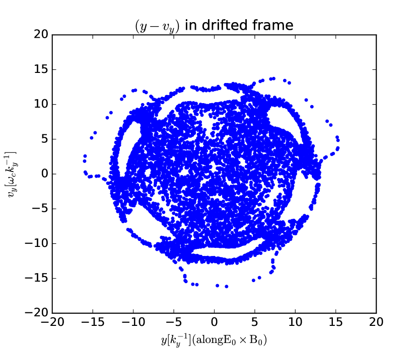
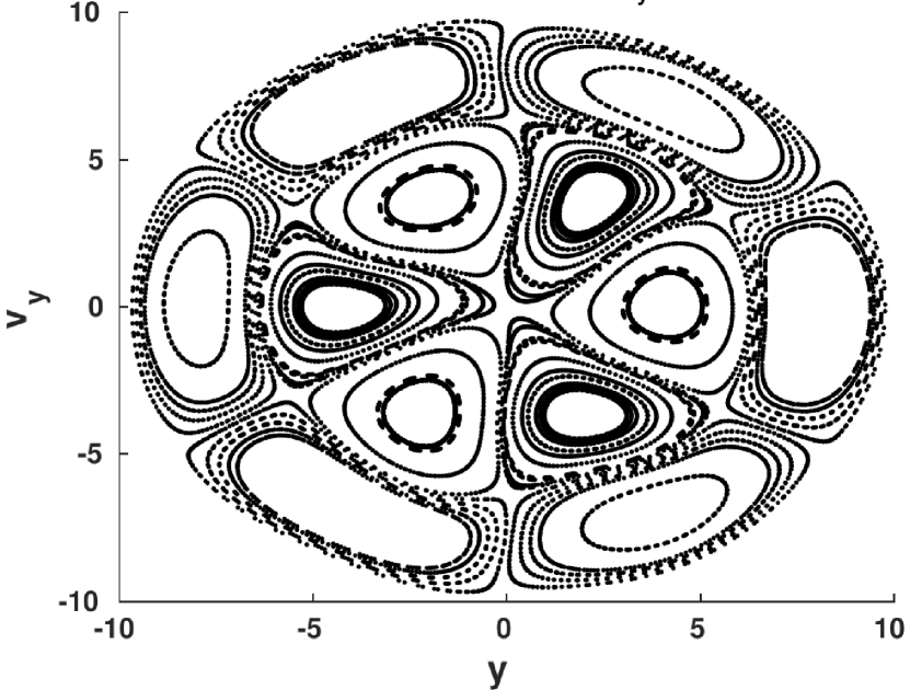
We first plot the stroboscopic Poincaré section in the $(Y^{\prime},P^{\prime}_{y})$ plane of a single particle trajectory at times $t=2n\pi/\nu_{1}$, where $n=0,1,2...$. The parameter $\varepsilon$ determines the radius of the stochastic web. The value of $\nu_{1}$ determines the shape of the web structure. For integer $\nu_{1}$, we observe a web structure with $\nu_{1}$-fold rotational symmetry (Figs 3 and 4). For parameters $(\varepsilon,\beta^{2},\nu_{1})=(0.69,1.83\cdot 10^{-5},1.39)$ with non-integer $\nu_{1}$, the dynamics generates a Halloween mask-like, deformed three-fold web structure (Fig. 5).

Along $Y^{\prime}$, the dynamics Eq. (12) has two time scales, one associated with the electrostatic wave (with period $2\pi/\nu_{1}$ in the drifting frame) and the other associated with a simple harmonic oscillator with period $2\pi$. Therefore, an integer value of $\nu_{1}$ causes resonance between these two time scales and one can eliminate the time dependence by taking the Poincaré section at a regular time interval, $nT=2\pi n/\nu_{1}$, to generate the stochastic web structures in the Poincaré section plot. The reduced frequency $\nu_{1}$ will determine the shape of the web structure.

For fixed values of $\varepsilon$, $\beta^{2}$ and $\nu_{1}$, any initial condition $(X^{\prime}_{0},Y^{\prime}_{0},{\dot{X}^{\prime}}_{0},{\dot{Y}^{\prime}}_{0})$, within the chaotic domain of the stochastic web, generates a similar web structure, and the particles with initial conditions outside the web structure and well inside the sticky islands (regions with no points in the web structures) generate regular trajectories.

In the time-independent Hamiltonian, $\dot{{\mathcal{X}}^{\prime}}={\dot{X}^{\prime}}-\nu_{1}$ and the dynamics depends on $(\varepsilon,\beta^{2})$ only. In this case, for any initial condition $({\mathcal{X}}^{\prime}_{0},{\mathcal{Y}}^{\prime}_{0},\dot{{\mathcal{X}}^{\prime}}_{0},\dot{{\mathcal{Y}}^{\prime}}_{0})$ within the chaotic domain of the stochastic web, the shape of the web structure depends on the initial $\dot{{\mathcal{X}}^{\prime}}_{0}$ values. For different $\dot{{\mathcal{X}}^{\prime}}_{0}$ values, the trajectory lies on different energy surfaces ${\mathcal{K}}=$ constant. Thus, particles with different initial conditions generate different web structures. Since $\beta^{2}\sim 10^{-6}$ in this study, the motion along the ${\mathcal{X}}^{\prime}$ direction is almost ballistic, $\dot{{\mathcal{X}}^{\prime}}\cong\textrm{constant}$. Therefore, we can generate Poincaré section plots by taking sections at ${\mathcal{X}}^{\prime}=n2\pi$, where $n$ is an integer.

Figs. 6 and 7 display the stroboscopic plot of the time-independent dynamics Eq. (15) with $(\varepsilon,\beta^{2})=(3.21,1.75\cdot 10^{-6})$ and two different initial velocities along the ${\mathcal{X}}^{\prime}$ direction, $\dot{{\mathcal{X}}}^{\prime}_{0}=3$ and $3.5$ respectively. For integer values of $\dot{{\mathcal{X}}^{\prime}}_{0}$ as in Fig. 6, the dynamics generates web structures similar to those generated in the Poincaré section plot for the cases of time-dependent dynamics (12) with same integer values of $\nu_{1}$. Fig. 7 presents the stroboscopic plot of a particle with $v_{0x}=3.5$, which corresponds to a higher-order resonance ($7/2$) : for fractional values of $\dot{{\mathcal{X}}^{\prime}}_{0}$, the stroboscopic plot generates different structures, because each of the different initial conditions lies on a different energy (${\mathcal{K}}={\rm{constant}}$) surface. Therefore, the web structures in the time-independent dynamics highly depend on the initial conditions of the particle.

In Figs. 8 and 9, we plot the distribution of

$$u_{i,n}=\bar{v}_{i}(n)-\langle v\rangle$$

(26)

for two different web structures, with $\nu_{1}=3$ and $\nu_{1}=6$, respectively. One can calculate the arc length for a time-independent dynamics also, but in the time-dependent dynamics, the parameter $\nu_{1}=(v_{\rm d}k_{y}-\omega_{1})/\omega_{c}$ is important in Hall thrusters. It expresses the frequency of the electrostatic modes generated by the ${\mathbf{E}}\times{\mathbf{B}}$ instability, in a frame which moves with the drift velocity $v_{\rm d}$ along the ${\mathbf{E}}_{0}\times{\mathbf{B}}_{0}$ direction. As our study is motivated by the anomalous chaotic transport in Hall thruster devices, we choose the time-dependent dynamics for characterising the transport for $\nu_{1}=3$ and $\nu_{1}=6$.

To characterize the transport, we consider two different stochastic webs corresponding to values $(3.21,1.75\cdot 10^{-6},3)$ and $(3.21,1.75\cdot 10^{-6},6)$ for parameters $(\varepsilon,\beta^{2},\nu_{1})$. We evolve the equations of motion (12) for 1024 particles with all initial conditions inside the chaotic domain, we calculate the arc length for each particle trajectory for a long time evolution ($10^{8}\,\omega_{{\mathrm{pe}}}^{-1}$) using a timestep value $\Delta t=3.33\cdot 10^{-3}\,\omega_{{\mathrm{c}}}^{-1}=3.33\cdot 10^{-2}\,\omega_{\rm{pe}}^{-1}$ in simulation, and we generate the distribution of the global average speed.

We plot the distribution at different times in Figs. 8 and 9 for both cases. To avoid nonphysical peaks in the distribution of $\rho_{n}$, the length $n$ of the time sequence should be sufficiently long for the dynamics to reach a saturation state, i.e.  for the Poincaré section of each particle’s trajectory to sample the whole phase space reach of the web. Here, we construct the distribution functions $\rho_{n}$ at times $t_{n}\geq 800\,\omega_{{\mathrm{pe}}}^{-1}$.

In the plot, the strong sharp peaks are associated with the stickiness phenomenon, by which a trajectory may remain for a long time close to the regular islands. The number of sharp peaks depends on the number of resonance generating sticky islands within the web structures, which we further discuss in the next section. We obtain more peaks for $\nu_{1}=6$ (Fig. 9) than for $\nu_{1}=3$ (Fig. 8). In the figure, $\log_{10}t=\log_{10}(n\tau_{\mathrm{P}})$, where $\tau_{\mathrm{P}}$ is the average time between two successive Poincaré sections. The relative magnitude of these sharp peaks decreases as $n\rightarrow\infty$, because the contribution from the chaotic domain becomes large compared to the contribution from the sticky regular trajectories as we consider a longer time evolution.

In both Figs. 8 and 9, the distribution after time $t_{n}\sim 10^{7}\,\omega_{{\mathrm{pe}}}^{-1}$ (yellow line) has almost zero relative strength of the sharp peaks, compared to the height of the smoother distribution. Stickiness generates a memory effect and Lévy flights leoncini04 . In absence of these sticky trajectories, the transport is purely diffusive and the exponent $\alpha$ takes the value $1/2$. In the presence of these sticky trajectories, the transport will be anomalous.

To measure $\alpha$, we find the value of $\rho_{\max}$ from the local maximum of the central smooth flat peak location which corresponds to the bulk and particles evolving in the chaotic domain, and not the sticky domains. In Fig. 10, we plot the time evolution of $\rho_{\max}$ for both cases $\nu_{1}=3$ and $\nu_{1}=6$. From the curve fitting, we obtain two different values $\alpha_{3}=0.17$ and $0.39$ for the case $\nu_{1}=3$ (magenta dashed line and data dots), and $\alpha_{6}=0.15$ and $0.33$ for $\nu_{1}=6$ (black). Both values of $\alpha$ in both cases are below $0.5$. Thus, the diffusion is anomalous and super-diffusive.

After a longer time evolution, most of the particles spend more time exploring the chaotic region of the stochastic web and sampling the ergodic measure. It appears that the contribution from the sticky islands “decreases” in comparison with the contribution from the chaotic domain, and that the “diffusion” rate increases at longer time ($t_{n}>10^{5}\,\omega_{{\mathrm{pe}}}^{-1}$). Note however that, even for large times, the exponent being smaller than 1/2 implies that the average speed fluctuations $\bar{v}_{i}-\langle v\rangle$ do not approach a Gaussian distribution, hence they do not obey the central limit theorem over this time scale, and transport is superdiffusive.

Similarly, we analyse transport for a stochastic web structure generated from the time-independent Hamiltonian with the corresponding arc length

$${\mathcal{S}}^{\prime}(t)=\int_{0}^{t}\sqrt{{\mathrm{d}}{\mathcal{X}}^{\prime 2}+{\mathrm{d}}{\mathcal{Y}}^{\prime 2}}.$$

(27)

Transport in web with simple rational parameter: The trajectories of 1024 particles are computed numerically up to time $10^{8}\,\omega_{{\mathrm{pe}}}^{-1}$ with time step $\Delta t=5.5\cdot 10^{-3}$. All particles are initially randomly distributed in $({\mathcal{X}}^{\prime},{\mathcal{Y}}^{\prime})$ plane within $-\pi\leq{\mathcal{X}}^{\prime}_{0}\leq\pi$ and $-\pi\leq{\mathcal{Y}}^{\prime}_{0}\leq\pi$. Their initial velocities along the ${\mathcal{Y}}^{\prime}$-direction are drawn from a Gaussian distribution with unit standard deviation. Along the ${\mathcal{X}}^{\prime}$-direction, we consider three different values $\dot{{\mathcal{X}}}^{\prime}_{0}=3$, $3.5$ and $6$ (simple rational) in order to analyse the transport in three different web structures generated from the time-independent Hamiltonian (15). For all three cases, we consider $\varepsilon=3.21$ and $\beta^{2}=1.75\cdot 10^{-6}$.

Figs. 11, 12 and 13 present the distribution of the average speed at different times for all three cases. Similarly to the time-dependent cases, sharp peaks in the distribution of average speed appear due to the presence of the sticky islands, and the number of sharp peaks is larger for the web structures with six-fold rotational symmetry, $\dot{{\mathcal{X}}^{\prime}_{0}}=6$, than for the three-fold rotational symmetry, $\dot{{\mathcal{X}}^{\prime}_{0}}=3$. In the case $\dot{{\mathcal{X}}^{\prime}_{0}}=3.5$, as seen in Fig. 7, the number and area of sticky islands are smaller than for $\dot{{\mathcal{X}}^{\prime}_{0}}=3$. Therefore, the height in the smooth part of the distribution, due to the chaotic domain, is larger for $\dot{{\mathcal{X}}^{\prime}_{0}}=3.5$.

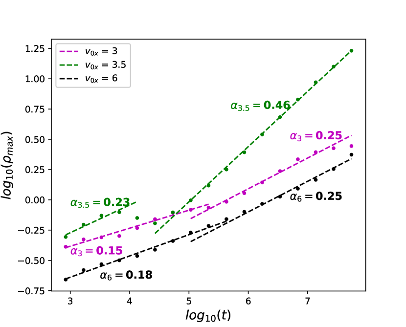
To estimate the exponent values from Eq. (24), we plot in Fig. 14 the time evolution of $\rho_{\max}$ for all three cases. For $\dot{{\mathcal{X}}}^{\prime}_{0}=3$ (magenta) and $6$ (black), the plots are similar to the time-dependent cases. From the curve fitting, we obtain two different values of $\alpha$ in two different regimes of the plots, $\alpha_{3}=(0.15,0.25)$ and $\alpha_{6}=(0.18,0.25)$. In both cases, the transport is anomalous of super-diffusive type. The values for the shorter time span ($t<5\cdot 10^{5}\,\omega_{{\mathrm{pe}}}^{-1}$) are very close to the values that are recovered for the time-dependent dynamics.

For fractional values of $\dot{{\mathcal{X}}}^{\prime}_{0}$, the number and area of the sticky islands are smaller than for the other two cases. Most of the region within the stochastic webs is part of the chaotic domain, therefore the height of the distribution increases at a higher rate than in the other two cases, as we increase the value of $n$. For $\dot{{\mathcal{X}}}^{\prime}_{0}=3.5=7/2$, we find higher exponent values, $\alpha_{3.5}=(0.23,0.46)$. At short time, the relative contribution from sticky trajectories is significantly large, which reduces the exponent value to $\alpha_{3.5}=0.23$ ; in contrast, for longer time $t>5\cdot 10^{4}\,\omega_{{\mathrm{pe}}}^{-1}$, the contribution from the chaotic region dominates over the contribution from sticky islands, and sharp peaks almost disappear, which increases the exponent value to $\alpha_{3.5}=0.46$, so that the transport becomes closer to a diffusive type.

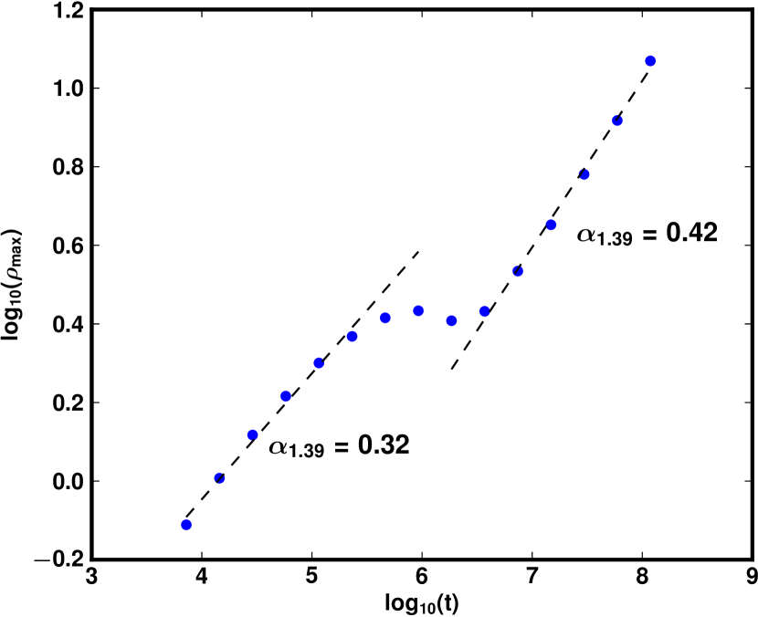
Transport in Halloween mask like web: For $\dot{{\mathcal{X}}^{\prime}}_{0}=1.39$ (further away from a simple rational) and $(\varepsilon,\beta^{2})=(0.69,1.83\cdot 10^{-5})$, we also draw 1024 initial conditions in the chaotic part of the domain defined by $-\pi\leq{\mathcal{X}}^{\prime}_{0}\leq\pi$, $\dot{{\mathcal{Y}}^{\prime}}_{0}$ a Gaussian random number with expectation 0 and standard deviation 1, and ${\mathcal{Y}}^{\prime}_{0}$ outside the islands (typically, $0.1\,\pi\leq|{\mathcal{Y}}^{\prime}_{0}|\leq 0.6\,\pi$). With these parameters and initial conditions, the same analysis applies, as seen from the peaks in the distribution in Fig. 15 and from the slopes $\alpha_{1.39}=(0.32,0.42)$ in Fig. 16. In the next section, we discuss this change of exponent values more quantitatively.

References

- (1) G. M. Zaslavsky, Chaos 1, 1 (1991), doi:10.1063/1.165811.
- (2) A. A. Chernikov, M. Ya. Natenzon, B. A. Petrovichev, R. Z. Sagdeev and G. M. Zaslavsky, Phys. Lett. A 122, 39 (1987), doi:10.1016/0375-9601(87)90772-9.
- (3) A. A. Vasil’ev and G. M. Zaslavsky, Sov. Phys. JETP 72, 826 (1991).
- (4) S. Benkadda, A. Sen and D. R. Shklyar, Chaos 6, 451 (1996), doi:10.1063/1.166187.
- (5) L. Chen, Z. Lin and R. White, Phys. Plasmas 8, 4713 (2001), doi:10.1063/1.1406939.
- (6) R. Balescu, Aspects of anomalous transport in plasmas, IoP Publishing (Bristol, 2005).
- (7) L. Bouchara, O. Ourrad, S. Vaienti and X. Leoncini, Chaos, Solitons and Fractals 78, 277 (2015), doi:10.1016/j.chaos.2015.08.007.
- (8) N. G. van Kampen, Stochastic processes in physics and chemistry, Elsevier (Amsterdam, 1992).
- (9) R. Balescu, Statistical dynamics – Matter out of equilibrium, Imperial College Press (London, 1997), doi:10.1142/p036.
- (10) B. Øksendal, Stochastic differential equations, 6th ed., Springer (Berlin, 2003).
- (11) B. V. Chirikov, Chaos, Solitons and Fractals 1, 79 (1991), doi:10.1016/0960-0779(91)90057-G.
- (12) L. A. Bunimovich and L. V. Vela-Arevalo, Chaos 25, 097614 (2015), doi:10.1063/1.4916330.
- (13) Č. Lozej and M. Robnik, Phys. Rev. E 98, 022220 (2018), doi:10.1103/PhysRevE.98.022220.
- (14) R. Balescu, Phys. Rev. E 51, 4807 (1995), doi:10.1103/PhysRevE.51.4807.
- (15) V. Méndez, D. Campos and F. Bartumeus, Stochastic Foundations in Movement Ecology – Anomalous Diffusion, Front Propagation and Random Searches, ch. 4, pp. 113-148. Springer (Heidelberg, 2014), doi:10.1007/978-3-642-39010-4_4.
- (16) M. F. Shlesinger, G. M. Zaslavsky and U. Frisch (eds), Lévy flights and related topics in physics (Nice, 27-30 June, 1994), Springer (Berlin, 1995).
- (17) D. del-Castillo-Negrete, Phys. Fluid, 10, 576 (1998), doi:10.1063/1.869585.
- (18) T. H. Solomon, E. R. Weeks and H. L. Swinney, Physica D 76, 70 (1994), doi:10.1016/0167-2789(94)90251-8.
- (19) A.H. Boozer, Phys. Lett. 185, 423 (1994), doi:10.1016/0375-9601(94)90178-3.
- (20) G. M. Zaslavsky, The physics of chaos in hamiltonian systems, 2nd ed., Imperial College Press (London, 2007).
- (21) G. Contopoulos and M. Harsoula, Int. J. Bif. Chaos 20, 2005–2043 (2010), doi:10.1142/S0218127410026915.
- (22) C. F. F. Karney, Phys. Fluids 21, 1584 (1978), doi:10.1063/1.862406.
- (23) C. F. F. Karney, Phys. Fluids 22, 2188 (1979), doi:10.1063/1.862512.
- (24) I. D. Kaganovich et al., arxiv.org/abs/2007.09194.
- (25) A. B. Mikhailovskii, Electromagnetic instabilities in an inhomogeneous plasma, transl. E. W. Laing, Institute of Physics Publishing (Bristol, 1992).
- (26) S. N. Abolmasov, Plasma Sources Sci. Technol. 21, 035006 (2012), doi:10.1088/0963-0252/21/3/035006.
- (27) J. P. Boeuf, J. Clauster, B. Chaudhury and G. Fubiani, Phys. Plasmas 19, 113510 (2012), doi:10.1063/1.4768804.
- (28) C. L. Ellison, Y. Raitses and N. J. Fisch, Phys. Plasmas 19, 013503 (2012), doi:10.1063/1.3671920.
- (29) M. Matsukuma, Th. Pierre, A. Escarguel, D. Guyomarc’h, G. Leclert, F. Brochard, E. Gravier and Y. Kawai, Phys. Lett. A 314, 163 (2003), doi:10.1016/S0375-9601(03)00865-X.
- (30) S. Marini and R. Pakter, Phys. Plasmas 24, 053507 (2017), doi:10.1063/1.4982685.
- (31) A. A. Skovoroda, E. A. Sorokina, and O. I. Podturova, Plasma Phys. Rep. 45, 941 (2019). doi:10.1134/S1063780X19100064.
- (32) D. Mandal, Y. Elskens, N. Lemoine and F. Doveil, Phys. Plasmas 27, 032301 (2020), doi:10.1063/1.5134148.
- (33) J. Cavalier, N. Lemoine, G. Bonhomme, S. Tsikata, C. Honoré and D. Grésillon, Phys. Plasmas 20, 082107 (2013), doi:10.1063/1.4817743.
- (34) J. P. Boeuf and L. Garrigues, Phys. Plasmas 25, 061204 (2018), doi:10.1063/1.5017033.
- (35) S. Tsikata, C. Honoré, N. Lemoine and D. M. Grésillon, Phys. Plasmas 17, 112110 (2010), doi:10.1063/1.3499350.
- (36) G. Benettin and F. Fassò, Appl. Numer. Math 29, 73 (1999).
- (37) E. Hairer, Ch. Lubich and G. Wanner, Acta Numerica 12, 399 (2003), doi:10.1017/S0962492902000144.
- (38) Y. Elskens and D. Escande, Microscopic dynamics of plasmas and chaos, IoP Publishing (Bristol, 2003).
- (39) X. Leoncini, C. Chandre and O. Ourrad, Comptes Rendus Mécanique 336, 530 (2008), doi:10.1016/j.crme.2008.02.006.
- (40) X. Leoncini, L. Kuznetsov and G. M. Zaslavsky, Chaos, Solitons and Fractals 19, 259 (2004), doi:10.1016/S0960-0779(03)00040-7.
- (41) B. Meziani, O. Ourrad and X. Leoncini, pp. 58-66 in X. Leoncini and M. Leonetti (eds), Chaos, Complexity and Transport, World Scientific (Singapore, 2012), doi:10.1142/9789814405645_0006.
- (42) Y. Elskens and D.F. Escande, Nonlinearity 4, 615 (1991), doi:10.1088/0951-7715/4/3/002.
- (43) Y. Elskens and D.F. Escande, Physica D 62, 66 (1993), doi:10.1016/0167-2789(93)90272-3.
- (44) A. Neishtadt, Nonlinearity 32, R53 (2019), doi:10.1088/1361-6544/ab2a2c.
- (45) T. Tél, Chaos 25, 097619 (2015), doi:10.1063/1.4917287.