STEERER: Resolving Scale Variations for Counting and Localization
via Selective Inheritance Learning
Abstract
Scale variation is a deep-rooted problem in object counting, which has not been effectively addressed by existing scale-aware algorithms. An important factor is that they typically involve cooperative learning across multi-resolutions, which could be suboptimal for learning the most discriminative features from each scale. In this paper, we propose a novel method termed STEERER (SelecTivE inhERitance lEaRning) that addresses the issue of scale variations in object counting. STEERER selects the most suitable scale for patch objects to boost feature extraction and only inherits discriminative features from lower to higher resolution progressively. The main insights of STEERER are a dedicated Feature Selection and Inheritance Adaptor (FSIA), which selectively forwards scale-customized features at each scale, and a Masked Selection and Inheritance Loss (MSIL) that helps to achieve high-quality density maps across all scales. Our experimental results on nine datasets with counting and localization tasks demonstrate the unprecedented scale generalization ability of STEERER. Code is available at https://github.com/taohan10200/STEERER.
1 Introduction
The utilization of computer vision techniques to count objects has garnered significant attention due to its potential in various domains. These domains include but are not limited to, crowd counting for anomaly detection [32, 5], vehicle counting for efficient traffic management [51, 81, 49], cell counting for accurate disease diagnosis [11], wildlife counting for species protection [2, 29], and crop counting for effective production estimation [43].

Numerous pioneers [38, 60, 3, 27, 74, 47, 22, 79, 24] have emphasized that the scale variations encountered in counting tasks present a formidable challenge, motivating the development of various algorithms aimed at mitigating their deleterious impact. These algorithms can be broadly classified into two branches: 1) Learn to scale methods [37, 78, 54] address scale variations in a two-step manner. Specifically, it involves estimating an appropriate scale factor for a given image/feature patch, followed by resizing the patch for prediction. Most of them require an additional training task (e.g., predicting the object’s scale) and the predicted density map is further partitioned into multiple parts, 2) Multi-scale fusion methods [36, 39] have been demonstrated to be effective in handling scale variations in various visual tasks, and their concept is also extensively utilized in object counting. Generally, they focus on two types of fusion, namely feature fusion [22, 79, 80, 59, 4, 61, 44, 50, 31, 83, 69] and density map fusion [10, 41, 25, 65, 42, 47, 63, 9]. Despite the recent progress, these studies still face challenges in dealing with scale variations, especially for large objects, as shown in Fig. 1. The main reason is that the existing multi-scale methods (e.g. FPN [36]) adapt the same loss to optimize all resolutions, which poses a great challenge for each resolution to find which scale range is easy to handle. Also, it results in mutual suppression because counting the same object accurately at all scales is hard.
Prior research [79, 41, 63] has revealed that different resolutions possess varying degrees of scale tolerance in a multi-resolution fusion network. Specifically, a single-resolution feature can accurately represent some objects within a limited scale range, but it may not be effective for other scales, as visualized in feature maps in Fig. 2 red boxes. We refer to features that can accurately predict object characteristics as scale-customized features; otherwise, they are termed as scale-uncustomized features. If scale-customized features can be separated from their master features before the fusion process, it is possible to preserve the discriminative features throughout the entire fusion process. Hence, our first motivation is to disentangle each resolution into scale-customized and scale-uncustomized features before each fusion, enabling them to be independently processed. To accomplish this, we introduce the Feature Selection and Inheritance Adaptor (FSIA), which comprises three sub-modules with independent parameters. Two adaptation modules separately process the scale-customized and the scale-uncustomized features, respectively, while a soft-mask generator attentively selects features in the middle.
Notably, conventional optimization methods do not ensure that FSIA acquires the desired specialized functions. Therefore, our second motivation is to enhance FSIA’s capabilities through exclusive optimization targets at each resolution. The first function of these objectives is to implement inheritance learning when transmitting the lower-resolution feature to a higher resolution. This process entails combining the higher-resolution feature with the scale-customized feature disentangled from the lower resolution, which preserves the ability to precisely predict larger objects that are accurately predicted at lower resolutions. Another crucial effect of these objectives is to ensure that each scale is able to effectively capture objects within its proficient scale range, given that the selection of the suitable scale-customized feature at each resolution is imperative for the successful implementation of inheritance learning.
In conclusion, our ultimate goal is to enhance the capabilities of FSIA through Masked Selection and Inheritance Loss (MSIL), which is composed of two sub-objectives controlled by two mask maps at each scale. To build them, we propose a Patch-Winner Selection Principle that automatically selects a proficient region mask for each scale. The mask is applied to the predicted and ground-truth density maps, enabling the selection of the effective region and filtering out other disturbances. Also, each scale inherits the mask from all resolutions lower than it, allowing for a gradual increase in the objective from low-to-high resolutions, where the incremental objective for a high resolution is the total objective of its neighboring low resolution. The proposed approach is called SeleceTivE inhERitance lEaRning (STEERER), where FSIA and MSIL are combined to maximize the scale generalization ability. STEERER achieves state-of-the-art counting results on several counting tasks and is also extended to achieve SOTA object localization. This paper’s primary contributions include:
-
•
We introduce STEERER, a principled method for object counting that resolves scale variations by cumulatively selecting and inheriting discriminative features from the most suitable scale, thereby enabling the acquisition of scale-customized features from diverse scales for improved prediction accuracy.
-
•
We propose a Feature Selection and Inheritance Adaptor that explicitly partitions the lower scale feature into its discriminative and undiscriminating components, which facilitates the integration of discriminative representations from lower to higher resolutions and their progressive transmission to the highest resolution.
-
•
We propose a Masked Selection and Inheritance Loss that utilizes the Patch-Winner Selection Principle to select the optimal scale for each region, thereby maximizing the discriminatory power of the features at the most suitable scales and progressively empowering FSIA with progressive constraints.
2 Related Work
2.1 Multi-scale Fusion Methods
Multi-scale Feature Fusion. This genre aims to address scale variations by leveraging multi-scale features or multi-contextual information [82, 55, 59, 6, 22, 79, 80, 59, 4, 61, 44, 50, 31, 83, 69]. They can be further classified into non-attentive and attentive fusion techniques. Non-attentive fusion methods, such as MCNN [82], employ multi-size filters to generate different receptive fields for scale variations. Similarly, Switch-CNN [55] utilizes a switch classifier to select the optimal column for a given patch. Attentive fusion methods, on the other hand, utilize a visual attention mechanism to fuse multi-scale features. For instance, MBTTBF [61] combines multiple shallow and deep features using a self-attention-based fusion module to generate attention maps and weight the four feature maps. Hossain et al. [20] propose a scale-aware attention network that automatically focuses on appropriate global and local scales.
Multi-scale Density Fusion. This approach not only adapts multi-scale features but also hierarchically merges multi-scale density maps to improve counting performance [10, 41, 25, 38, 65, 42, 47, 63, 9, 26]. Visual attention mechanisms are utilized to regress multiple density maps and extra weight/attention maps [10, 25, 63] during both training and inference stages. For example, DPN-IPSM [47] proposes a weakly supervised probabilistic framework that estimates scale distributions to guide the fusion of multi-scale density maps. On the other hand, Song et al. [63] propose an adaptive selection strategy to fuse multiple density maps by selecting region-aware hard pixels through a PRALoss and optimizing them in a fine-grained manner.
2.2 Learn to Scale Methods
These studies typically employ a single-resolution architecture but utilize auxiliary tasks to learn a tailored factor for resizing the feature or image patch to refine the prediction. The final density map is a composite of the patch predictions. For instance, Liu et al. [37] propose the Recurrent Attentive Zooming Network, which iteratively identifies regions with high ambiguity and evaluates them in high-resolution space. Similarly, Xu et al. [78] introduce a Learning to Scale module that automatically resizes regions with high density for another prediction, improving the quality of the density maps. ZoomCount [54] categorizes image patches into three groups based on density levels and then uses specially designed patch-makers and crowd regressors for counting.
Differences with Previous. The majority of scale-aware methods adopt a divide-and-conquer strategy, which is also employed in this study. However, we argue that this does not diminish the novelty of our work, as it is a fundamental thought in numerous computer vision works. Our technical designs significantly diverge from the aforementioned methods and achieve better performance. Typically, Kang et al. [26] attempts to alter the scale distribution by inputting multi-scale images. In contrast, our method disentangles the most suitable features from multi-resolution representation without multi-resolution inputs, resulting in a distinct general structure. Additionally, some methods [26, 78] require multiple forward passes during inference, while our method only requires a single forward pass.

3 Selective Inheritance Learning
3.1 Multi-resolution Feature Representation
Multi-resolution features are commonly adapted in deep learning algorithms to capture multi-scale objects. The feature visualizations in the red boxes depicted in Fig. 2 demonstrate that lower-resolution features are highly effective at capturing large objects, while higher-resolution features are only sensitive to small-scale objects. Therefore, building multi-resolution feature representations is critical. Specifically, let be the input RGB image, and denotes the backbone network, where represents its parameters. We use to represent multi-feature representations, where the th level’s spatial resolution is , and represents the lowest resolution feature. The fusion process proceeds from the bottom to the top. This paper primarily utilizes HRNet-W48 [68] as the backbone, as its multi-resolution features have nearly identical depths. Additionally, some extended experiments based on the VGG-19 backbone [57] are conducted to generalize STEERER.
3.2 Feature Selection and Inheritance Adaptor
Fig. 2 exemplifies that the feature of large objects in level is the most aggregated and most dispersive in level . Directly upsampling the lowest feature and fusing it to a higher resolution has two drawbacks and we propose FSIA to handle them: 1) the upsampling operations can degrade the scale-customized feature at each resolution, leading to reduced confidence for large objects, as depicted in the middle image of Fig. 1; 2) the dispersive feature of large objects constitutes noise in higher resolution, and vice versa.
Structure and Functions. The FSIA module, depicted in the lower left corner of Fig. 2, comprises three components that are learnable, where the scale-Customized feature Forward Network (CFN) and the scale-Uncustomized feature Forward Network (UFN), represented as and respectively. They both contain two convolutional layers followed by batch normalization and the Rectified Linear Unit (ReLU) activation function. The Soft-Mask Generator (SMG), , parameterized by , is composed of three convolutional layers. The CFN is responsible for combining the upsampled scale-customized features. The UFN, on the other hand, continuously forwards scale-uncustomized features to higher resolutions since they may be potentially beneficial for future disentanglement. If these features are not necessary, the UFN can still suppress them, minimizing their impact. The SMG actively identifies and generates two attention maps for feature disentanglement. Their relationships can be expressed as follows:
| (1) |
where C is the feature concatenation, and is a two-channel attention map. It is split into and along the channel dimension. is the Hadamard product. The fusion process begins with the last resolution, where the initial is set to . The input streams for the FSIA are and . The output streams are and with the same spatial resolution as . , and all have an inner upsampling operation. Notably, in the highest resolution, only the CFN is activated as the features are no longer required to be passed to subsequent scales.
3.3 Masked Selection and Inheritance Loss
FSIA is supposed to be trained toward its functions by imposing some constraints. In essence, our assumptions for addressing scale variations are 1) Each resolution can only yield good features within a certain scale range. and 2) For the objects belong to the same category, an implicit ground-truth feature distribution , exists that can be used to infer a ground-truth density map by forwarding it to a well-trained counting head. If is available, then the scale-customized feature can be accurately selected from and constrained appropriately. However, since the is impossible to figure out, we resort to masking the ground-truth density map for feature selection. To achieve this, we introduce a counting head , with being its parameter that is trained solely by the final output branch and kept frozen in other resolutions. By utilizing identical parameters, the feature pattern that can estimate the ground-truth Gaussian kernel is the same at every resolution. For instance, considering the FSIA depicted in Fig. 2 at the level, we first posit an ideal mask that accurately determines which regions in the level are most appropriate for prediction in comparison to other resolutions. Then the feature selection in level is implemented as,
| (2) |
where is the ground truth map. The substitute of the ideal will be elaborated in the PWSP subsection. With such a regulation, level will focus on the objects that have the closest distribution with ground truth. Apart from selection ability, level also requires inheriting the scale-customized feature upsampled from level. So another objective in level is to re-evaluate the most suitable regions in . That is, we defined on feature level to inherit the scale-customized feature from ,
| (3) |
where U performs upsampling operation to make the have the same spatial resolution as .
Hereby, the feature selection and inheritance are supervised by and , respectively. The inheritance loss activates the FSIA, which enables SMG to disentangle the resolution. Simultaneously, it also ensures that the fused feature , which combines the level with the scale-customized feature from , retains the ability to provide a refined prediction, as achieved by the level. The remaining FSIAs operate similarly, leading to hierarchical selection and inheritance learning. Finally, all objects are aggregated at the highest resolution for the final prediction.
Patch-Winner Selection Principle. Another crucial step is about how to determine the ideal mask in Eq. 2 and Eq. 3 for each level. Previous studies [78, 54, 47] employ scale labels to train scale-aware counting methods, where the scale label is generated in accordance with the geometric distribution [47, 46] or density level [25, 54, 59, 78]. However, they only approximately hold when the objects are evenly distributed. Thus, instead of generating by manually setting hyperparameters, we propose to allow the network to determine the scale division on its own. That is, each resolution automatically selects the most appropriate region as a mask. Our counting method is based on the popular density map estimation approach [30, 53, 77, 72, 19], which transfers point annotations into a 2D Gaussian-kernel based density map as ground-truth. As depicted in Fig. 2, the th resolution has a ground-truth density map denoted as , where is divided by a down-sampling factor in each scale.

| Method | Venue | Overall | Scene Level (MAE) | Luminance (MAE) | ||||||||||
| MAE | MSE | NAE | Avg. | S0 | S1 | S2 | S3 | S4 | Avg. | L0 | L1 | L2 | ||
| MCNN [82] | CVPR16 | 232.5 | 714.6 | 1.063 | 1171.9 | 356.0 | 72.1 | 103.5 | 509.5 | 4818.2 | 220.9 | 472.9 | 230.1 | 181.6 |
| CSRNet [33] | CVPR18 | 121.3 | 387.8 | 0.604 | 522.7 | 176.0 | 35.8 | 59.8 | 285.8 | 2055.8 | 112.0 | 232.4 | 121.0 | 95.5 |
| CAN [40] | CVPR19 | 106.3 | 386.5 | 0.295 | 612.2 | 82.6 | 14.7 | 46.6 | 269.7 | 2647.0 | 102.1 | 222.1 | 104.9 | 82.3 |
| BL [46] | ICCV19 | 105.4 | 454.2 | 0.203 | 750.5 | 66.5 | 8.7 | 41.2 | 249.9 | 3386.4 | 115.8 | 293.4 | 102.7 | 68.0 |
| SFCN+ [70] | PAMI20 | 105.7 | 424.1 | 0.254 | 712.7 | 54.2 | 14.8 | 44.4 | 249.6 | 3200.5 | 106.8 | 245.9 | 103.4 | 78.8 |
| DM-Count [67] | NeurIPS20 | 88.4 | 388.6 | 0.169 | 498.0 | 146.7 | 7.6 | 31.2 | 228.7 | 2075.8 | 88.0 | 203.6 | 88.1 | 61.2 |
| UOT [48] | AAAI21 | 87.8 | 387.5 | 0.185 | 566.5 | 80.7 | 7.9 | 36.3 | 212.0 | 2495.4 | 95.2 | 240.3 | 86.4 | 54.9 |
| GL [66] | CVPR21 | 79.3 | 346.1 | 0.180 | 508.5 | 92.4 | 8.2 | 35.4 | 179.2 | 2228.3 | 85.6 | 216.6 | 78.6 | 48.0 |
| D2CNet [7] | IEEE-TIP21 | 85.5 | 361.5 | 0.221 | 539.9 | 52.4 | 10.8 | 36.2 | 212.2 | 2387.8 | 82.0 | 177.0 | 83.9 | 68.2 |
| P2PNet [62] | ICCV21 | 72.6 | 331.6 | 0.192 | 510.0 | 34.7 | 11.3 | 31.5 | 161.0 | 2311.6 | 80.6 | 203.8 | 69.6 | 50.1 |
| MAN [35] | CVPR22 | 76.5 | 323.0 | 0.170 | 464.6 | 43.3 | 8.5 | 35.3 | 190.9 | 2044.9 | 76.4 | 180.1 | 77.1 | 49.4 |
| Chfl [56] | CVPR22 | 76.8 | 343.0 | 0.171 | 470.0 | 56.7 | 8.4 | 32.1 | 195.1 | 2058.0 | 85.2 | 217.7 | 74.5 | 49.6 |
| STEERER-VGG19 | - | 68.3 | 318.4 | 0.165 | 438.2 | 61.9 | 8.3 | 29.5 | 159.0 | 1932.1 | 71.0 | 171.3 | 67.4 | 46.2 |
| STEERER-HRNet | - | 63.7 | 309.8 | 0.133 | 410.6 | 48.2 | 6.0 | 25.8 | 158.3 | 1814.5 | 65.1 | 155.7 | 63.3 | 42.5 |
In detail, we propose a Patch-Winner Selection Principle (PWSP) to let each resolution select its capable region, whose thought is to find which resolution has the minimum cost for a given patch. During the training phase, each resolution outputs its predicted density map , where it is with the same spatial resolution as . As shown in Fig. 3, each pair of and are divided into regions, where , is the patch size, and we empirically set the patch size . (Note that the image will be padded to be divisible by this patch size during inference.) PWSP finally decides the best resolution for a given patch by comparing a re-weighted loss among four resolutions, which is defined as Eq. 4,
| (4) |
where the first item is the Averaged Mean Square Error (AMSE) between ground-truth density patch and predicted density patch , and the second item is the Instance Mean Square Error (IMSE). AMSE inclines to measure the overall difference, and it still works when a patch has no object, whereas IMSE gives emphasis on the foreground. is a very small number to prevent pointless division.
Total Optimization Loss. PWSP dynamically gets the region selection label . Fig. 3 shows that are transferred to mask with a one-hot encoding operation and an upsampling operation, namely, , where and . Hereby, the final scale selection and inherit mask for each resolution is obtained by Eq. 5,
| (5) |
where is resolution number and , Finally, is interpolated to be in Eq. 2 and Eq. 3, namely , which has the same spatial dimension with and . The and in Eq. 2 and Eq. 3 can be summed to a single loss by adding their masked weight. The ultimate optimization objective for STEERER is:
| (6) |
where is the weight at each resolution, and we empirically set it as . is the Euclidean distance.
| Method | SHHA | SHHB | UCF-QNRF | JHU-CROWD++ | ||||
|---|---|---|---|---|---|---|---|---|
| MAE | MSE | MAE | MSE | MAE | MSE | MAE | MSE | |
| CAN [40] | 62.3 | 100.0 | 7.8 | 12.2 | 107.0 | 183.0 | 100.1 | 314.0 |
| SFCN [71] | 64.8 | 107.5 | 7.6 | 13.0 | 102.0 | 171.4 | 77.5 | 297.6 |
| S-DCNet [76] | 58.3 | 95.0 | 6.7 | 10.7 | 104.4 | 176.1 | - | - |
| BL [46] | 62.8 | 101.8 | 7.7 | 12.7 | 88.7 | 154.8 | 75.0 | 299.9 |
| ASNet [25] | 57.8 | 90.1 | - | - | 91.6 | 159.7 | - | - |
| AMRNet [42] | 61.5 | 98.3 | 7.0 | 11.0 | 86.6 | 152.2 | - | - |
| DM-Count [67] | 59.7 | 95.7 | 7.4 | 11.8 | 85.6 | 148.3 | - | - |
| GL [66] | 61.3 | 95.4 | 7.3 | 11.7 | 84.3 | 147.5 | - | - |
| D2CNet [7] | 57.2 | 93.0 | 6.3 | 10.7 | 81.7 | 137.9 | 73.7 | 292.5 |
| P2PNet [62] | 52.7 | 85.1 | 6.3 | 9.9 | 85.3 | 154.5 | - | - |
| SDA+DM [45] | 55.0 | 92.7 | - | - | 80.7 | 146.3 | 59.3 | 248.9 |
| MAN [35] | 56.8 | 90.3 | - | - | 77.3 | 131.5 | 53.4 | 209.9 |
| Chfl [56] | 57.5 | 94.3 | 6.9 | 11.0 | 80.3 | 137.6 | 57.0 | 235.7 |
| RSI-ResNet50 [8] | 54.8 | 89.1 | 6.2 | 9.9 | 81.6 | 153.7 | 58.2 | 245.1 |
| STEERER-VGG19 | 55.6 | 87.3 | 6.8 | 10.7 | 76.7 | 135.1 | 55.4 | 221.4 |
| STEERER-HRNet | 54.5 | 86.9 | 5.8 | 8.5 | 74.3 | 128.3 | 54.3 | 238.3 |

4 Experimentation
4.1 Experimental Settings
Datasets. STEERER is comprehensively evaluated with object counting and localization experiments on nine datasets: NWPU-Crowd [70], SHHA [82], SHHB [82], UCF-QNRF [23], FDST [12], JHU-CROWD++ [58], MTC [43], URBAN_TREE [64], TRANCOS [16].
Implementation Details. We employ the Adam optimizer [28], with the learning rate gradually increasing from to during the initial 10 epochs using a linear warm-up strategy, followed by a Cosine decay strategy. Our approach is implemented using the PyTorch framework [52] on a single NVIDIA Tesla A100 GPU.
Evaluation Metrics. For object counting, Mean Absolute Error (MAE) and Mean Square Error (MSE) are used as evaluation measurements. For localization, we follow the NWPU-Crowd [70] localization challenge to calculate instance-level Precision, Recall, and F1-measure to evaluate models. All criteria are defined in the supplementary.
4.2 Object Counting Results
Crowd Counting. NWPU-Crowd benchmark is a challenging dataset with the largest scale variations, which provides a fair platform for evaluation. Tab. 1 compares STEERER with the CNN-based SoTAs. STEERER, based on VGG-19 and the HRNet backbone, both outperform other approaches on most of the counting metrics. On the whole, STEERER improves the MAE across all the sub-categories except for the level and overall dataset consistently. In detail, STEERER reduces the MAE to 63.7 on the NWPU-Crowd test set, which is reduced by compared with the second-place P2PNet [62]. Note that we currently rank No.1 on the public leaderboard of the NWPU-Crowd benchmark. On other crowd counting datasets, such as SHHA, SHHB, UCF-QNRF, and JHU-CROWD++, STEERER also achieves excellent performance compared with SoTAs.
| Method | Backbone | Overall () | Box Level (only Rec under ) (%) | |||
|---|---|---|---|---|---|---|
| F1-m(%) | Pre(%) | Rec(%) | Avg. | Head Area: | ||
| VGG+GPR [15, 13] | VGG-16 | 52.5 | 55.8 | 49.6 | 37.4 | 3.1/27.2/49.1/68.7/49.8/26.3 |
| RAZ_Loc [37] | VGG-16 | 59.8 | 66.6 | 54.3 | 42.4 | 5.1/28.2/52.0/79.7/64.3/25.1 |
| Crowd-SDNet [73] | ResNet-50 | 63.7 | 65.1 | 62.4 | 55.1 | 7.3/43.7/62.4/75.7/71.2/70.2 |
| TopoCount [1] | VGG-16 | 69.2 | 68.3 | 70.1 | 63.3 | 5.7/39.1/72.2/85.7/87.3/89.7 |
| FIDTM [34] | HRNet | 75.5 | 79.8 | 71.7 | 47.5 | 22.8/66.8/76.0/71.9/37.4/10.2 |
| IIM [14] | HRNet | 76.0 | 82.9 | 70.2 | 49.1 | 11.7/45.3/73.4/83.0/64.5/16.7 |
| LDC-Net [18] | HRNet | 76.3 | 78.5 | 74.3 | 56.6 | 14.8/53.0/77.0/85.2/70.8/39.0 |
| STEERER | HRNet | 77.0 | 81.4 | 73.0 | 61.3 | 12.0/46.0/73.2/85.5/86.7/64.3 |
| Method | Backbone | ShanghaiTech Part A | ShanghaiTech Part B | UCF-QNRF | FDST | ||||||||
|---|---|---|---|---|---|---|---|---|---|---|---|---|---|
| F1-m | Pre. | Rec. | F1-m | Pre. | Rec. | F1-m | Pre. | Rec. | F1-m | Pre. | Rec. | ||
| TinyFaces [21] | ResNet-101 | 57.3 | 43.1 | 85.5 | 71.1 | 64.7 | 79.0 | 49.4 | 36.3 | 77.3 | 85.8 | 86.1 | 85.4 |
| RAZ_Loc [37] | VGG-16 | 69.2 | 61.3 | 79.5 | 68.0 | 60.0 | 78.3 | 53.3 | 59.4 | 48.3 | 83.7 | 74.4 | 95.8 |
| LSC-CNN [3] | VGG-16 | 68.0 | 69.6 | 66.5 | 71.2 | 71.7 | 70.6 | 58.2 | 58.6 | 57.7 | - | - | - |
| IIM [14] | HRNet | 73.3 | 76.3 | 70.5 | 83.8 | 89.8 | 78.6 | 71.8 | 73.7 | 70.1 | 95.4 | 95.4 | 95.3 |
| STEERER | HRNet | 79.8 | 80.0 | 79.4 | 87.0 | 89.4 | 84.8 | 75.5 | 78.6 | 72.7 | 96.8 | 96.6 | 97.0 |
Plant and Vehicle Counting. Tab. 5 shows STEERER works well when directly applying it to evaluate the vehicle (TRANCOS [16]) and Maize counting (MTC [43]). For vehicle counting, we further lower the estimated MAE. For plant counting, our model surpasses other SoTAs, whose MAE and MSE are decreased by and , respectively, which shows significant improvements.
4.3 Object Localization Results
Crowd Localization. STEERER, benefiting from its high-resolution and elaborated density map, can use a heuristic localization algorithm to locate the object center. Specifically, we follow DRNet [17] to extract the local maximum as a head position from the predicted density map. Tab. 3 tabulates the overall performances (Localization: F1-m, Pre. and Rec.) and per-class Rec. at the box level. By comparing the primary key (Overall F1-m) for ranking, our method achieves first place on the F1-m 77.0% compared with other crowd localization methods. Notably, Per-class Rec. on Box Level shows the sensitivity of the model for scale variations. The box-level results show our method achieves a balanced performance on all scales (A0A5), which further verifies the effectiveness of STEERER for addressing scale variations. Tab. 4 lists the localization results on other datasets. Here, we adopt the same evaluation protocol with IIM [14]. Tab. 4 demonstrates that STEERER refreshes the F1-measure on all datasets. In general, our localization results precede other SoTA methods. Take F1-m as an example. The relative performance of our method is increased by an average of on these four datasets.
Urban Tree Localization. URBANTREEC [64] collects trees in urban environments with aerial imagery. As presented in Tab. 6, ITC [64] takes multi-spectral imagery as input and outputs a confidence map indicating the locations of trees. The individual tree locations are found by local peak finding. Similarly, the predicted density map in our framework can also be used to locate the urban trees in this way. Our method achieves a significant improvement over the RGB format in ITC [64], with of the detected trees matching actual trees, and of the trees area being detected, despite using fewer input channels.
4.4 Ablation Study
The ablations quantitatively compare the contribution of each component. Here, we set our two baselines as, 1) BL1: Upsample and concatenate them to the first branch. 2)BL2: Using FPN [36] to make bottom-to-up fusion.
Effectiveness of FSIA. We here compare the proposed FSIA with the traditional fusion methods, namely BL1 and BL2. LABEL:tab:fusion_methods shows that the proposed fusion method is able to catch more objects with less computation. Furthermore, FSIA has the utmost efficiency when three components of FSIA are combined into a unit.
Effectiveness of Hierarchy Constrain. LABEL:tab:loss_conbination shows that imposing the scale selection and inheritance loss on each resolution can improve performance step by step. The best performance requires optimizing on all resolutions.
Effectiveness of MSIL. LABEL:tab:mask_ablation explores the necessity of both selection and inheritance at each scale. If we simply force each scale to ambiguously learn all objects (LABEL:tab:mask_ablation Row 1), FISM does not achieve the function that we want. If we only select the most suitable patch for each scale to learn, it would be crashed (Row 2). So we conclude that selection and inheritance are indispensable in our framework.
Effectiveness of Head Sharing. The shared counting head ensures that each scale selects its proficient regions equitably. Otherwise, it does not work, as evident from the head-dependent results presented in LABEL:tab:mask_ablation. More ablation experiments and baseline results are provided in the supplementary.
| Fusion method | MAE | MSE | FLOPs |
|---|---|---|---|
| BL1-Concat | 60.4 | 98.5 | 1.21 |
| BL2-FPN [36] | 60.4 | 96.3 | 1.16 |
| CFN | 55.3 | 89.7 | 0.99 |
| UFN+CFN | 55.1 | 90.5 | 0.99 |
| UFN+CFN+SMG | 54.6 | 86.9 | 1.00 |
| MAE | MSE | |
|---|---|---|
| 58.4 | 92.0 | |
| + | 56.5 | 92.8 |
| ++ | 55.8 | 88.1 |
| +++ | 54.6 | 86.9 |
| Mask type | MAE | MSE |
| No mask | 60.5 | 99.7 |
| 675.4 | 809.6 | |
| + | 54.6 | 86.9 |
| head-dependent | 329.2 | 396.5 |
| head-sharing | 54.6 | 86.9 |

4.5 Visualization Analysis
Convergence Comparison. Fig. 5 depicts the change of MAE on NWPU-Crowd val set during training. STEERER and two baselines are trained with the same configuration. This comparison demonstrates that STEERER converges to a lower local minimum with faster speed.
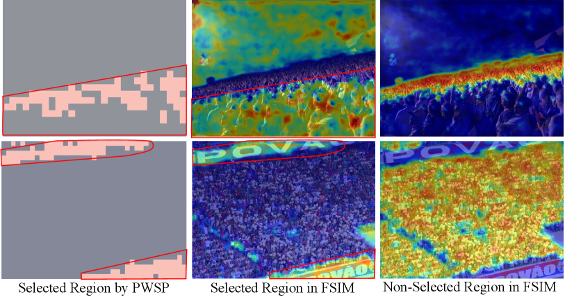
Attentively Visualize FSIA. Fig. 6 shows FSIA’s selected results at resolution. The medium Class Activate Map [84] demonstrates FSIA only selects the large objects in this scale, which aligns with the mask assigned by PWSP. The highlighted regions in the right figures mean objects are small and will be forwarded to a higher resolution.
Visualization Results. Fig. 4 pictures the quality of the density map and the localization outcomes in practical scenarios. In the crowd scene, both STEERER and the baseline models exhibit superior accuracy in generating density maps in comparison to AutoScale [78]. Regarding object localization, STEERER displays greater generalizability in detecting large objects in contrast to the baseline and P2PNet [62], as evidenced by the red box in Fig. 4. Additionally, STEERER maintains its efficacy in identifying small and dense objects (see the yellow box in Fig. 4). Remarkably, the proposed STEERER model exhibits transferability across different domains, such as vehicle, tree, and maize localization and counting.
4.6 Cross Dataset Evaluation
This cross-dataset testing demonstrates its generalization ability when it comes across scale variations. In Tab. 8, the baseline model and the proposed model are trained on SHHA (medium scale variations), and then their performance is evaluated on QNRF (large scale variations), and vice versa. Evidently, our method has a higher generalization ability than the FPN [36] fusion method. Surprisingly, our model trained on QNRF with STEERER achieves comparable results with the SoTA results in Tab. 2.
4.7 Discussions
Inherit from the lowest resolution. Fusing from the lowest resolution can hierarchically constrain the density of large objects, while gradually adding the smaller objects. Otherwise, the congested object would be significantly overlapped and challenging to disentangle.
Only output density in the highest resolution. STEERER can integrate multiple-resolution prediction maps by leveraging the attention map embedded within FSIM to weigh and aggregate the predictions. However, its counting performance on the SHHA dataset, with an MAE/MSE of 63.4/102.5, falls short of the highest resolution’s result of 54.5/86.9. Also, the highest resolution yields essential details and granularity required for accurate localization in crowded scenes, as exemplified in 4.3.
5 Conclusion
In this paper, we propose a selective inheritance learning method to dexterously resolve the scale variations in object counting. Our method, STEERER, first selects the most suitable region autonomously for each resolution with the proposed PWSP and then disentangles the lower resolution feature into scale-customized and scale-uncustomized components by the proposed FSIA in front of the fusion. The scale-customized part is combined with higher resolution to re-estimate the selected region by the last scale and the self-selected region, where those two processes are compacted into selection and inheritance. The experiment results show that our method plays favorably against state-of-the-art approaches with object counting and localization tasks. Notably, we believe the thoughts behind STEERER can inspire more works to address scale variations in other vision tasks.
| Setting | Method | MAE | MSE | NAE |
|---|---|---|---|---|
| SHHA QNRF | BL2 | 120.3 | 224.5 | 0.1744 |
| STEERER | 109.4 | 203.4 | 0.149 | |
| QNRF SHHA | BL2 | 58.8 | 99.7 | 0.138 |
| STEERER | 54.1 | 91.2 | 0.124 |
Acknowledgement. This work is partially supported by the National Key R&D Program of China(NO.2022ZD0160100), and in part by Shanghai Committee of Science and Technology (Grant No. 21DZ1100100).
References
- [1] Shahira Abousamra, Minh Hoai, Dimitris Samaras, and Chao Chen. Localization in the crowd with topological constraints. arXiv preprint arXiv:2012.12482, 2020.
- [2] Carlos Arteta, Victor Lempitsky, and Andrew Zisserman. Counting in the wild. In ECCV, pages 483–498. Springer, 2016.
- [3] Deepak Babu Sam, Skand Vishwanath Peri, Mukuntha Narayanan Sundararaman, Amogh Kamath, and Venkatesh Babu Radhakrishnan. Locate, size and count: Accurately resolving people in dense crowds via detection. IEEE TPAMI, 2020.
- [4] Xinkun Cao, Zhipeng Wang, Yanyun Zhao, and Fei Su. Scale aggregation network for accurate and efficient crowd counting. In ECCV, pages 734–750, 2018.
- [5] Rima Chaker, Zaher Al Aghbari, and Imran N Junejo. Social network model for crowd anomaly detection and localization. RP, 61:266–281, 2017.
- [6] Xinya Chen, Yanrui Bin, Nong Sang, and Changxin Gao. Scale pyramid network for crowd counting. In WACV, pages 1941–1950. IEEE, 2019.
- [7] Jian Cheng, Haipeng Xiong, Zhiguo Cao, and Hao Lu. Decoupled two-stage crowd counting and beyond. IEEE TIP, 30:2862–2875, 2021.
- [8] Zhi-Qi Cheng, Qi Dai, Hong Li, Jingkuan Song, Xiao Wu, and Alexander G Hauptmann. Rethinking spatial invariance of convolutional networks for object counting. In CVPR, pages 19638–19648, 2022.
- [9] Zhi-Qi Cheng, Jun-Xiu Li, Qi Dai, Xiao Wu, and Alexander G Hauptmann. Learning spatial awareness to improve crowd counting. In CVPR, pages 6152–6161, 2019.
- [10] Zhipeng Du, Miaojing Shi, Jiankang Deng, and Stefanos Zafeiriou. Redesigning multi-scale neural network for crowd counting. arXiv preprint arXiv:2208.02894, 2022.
- [11] Furkan Eren, Mete Aslan, Dilek Kanarya, Yigit Uysalli, Musa Aydin, Berna Kiraz, Omer Aydin, and Alper Kiraz. Deepcan: A modular deep learning system for automated cell counting and viability analysis. IEEE JBHI, 2022.
- [12] Yanyan Fang, Biyun Zhan, Wandi Cai, Shenghua Gao, and Bo Hu. Locality-constrained spatial transformer network for video crowd counting. In ICME, pages 814–819. IEEE, 2019.
- [13] Junyu Gao, Tao Han, Qi Wang, and Yuan Yuan. Domain-adaptive crowd counting via inter-domain features segregation and gaussian-prior reconstruction. arXiv preprint arXiv:1912.03677, 2019.
- [14] Junyu Gao, Tao Han, Yuan Yuan, and Qi Wang. Learning independent instance maps for crowd localization. arXiv preprint arXiv:2012.04164, 2020.
- [15] Junyu Gao, Wei Lin, Bin Zhao, Dong Wang, Chenyu Gao, and Jun Wen. C3 framework: An open-source pytorch code for crowd counting. arXiv preprint arXiv:1907.02724, 2019.
- [16] Ricardo Guerrero-Gómez-Olmedo, Beatriz Torre-Jiménez, Roberto López-Sastre, Saturnino Maldonado-Bascón, and Daniel Onoro-Rubio. Extremely overlapping vehicle counting. In PRIA, pages 423–431. Springer, 2015.
- [17] Tao Han, Lei Bai, Junyu Gao, Qi Wang, and Wanli Ouyang. Dr.vic: Decomposition and reasoning for video individual counting. In CVPR, pages 3083–3092, 2022.
- [18] Tao Han, Junyu Gao, Yuan Yuan, Xuelong Li, et al. Ldc-net: A unified framework for localization, detection and counting in dense crowds. arXiv preprint arXiv:2110.04727, 2021.
- [19] Tao Han, Junyu Gao, Yuan Yuan, and Qi Wang. Focus on semantic consistency for cross-domain crowd understanding. In ICASSP, pages 1848–1852. IEEE, 2020.
- [20] Mohammad Hossain, Mehrdad Hosseinzadeh, Omit Chanda, and Yang Wang. Crowd counting using scale-aware attention networks. In WACV, pages 1280–1288. IEEE, 2019.
- [21] Peiyun Hu and Deva Ramanan. Finding tiny faces. In CVPR, pages 951–959, 2017.
- [22] Haroon Idrees, Imran Saleemi, Cody Seibert, and Mubarak Shah. Multi-source multi-scale counting in extremely dense crowd images. In Proceedings of the IEEE conference on computer vision and pattern recognition, pages 2547–2554, 2013.
- [23] Haroon Idrees, Muhmmad Tayyab, Kishan Athrey, Dong Zhang, Somaya Al-Maadeed, Nasir Rajpoot, and Mubarak Shah. Composition loss for counting, density map estimation and localization in dense crowds. In ECCV, pages 532–546, 2018.
- [24] Rui Jiang, Ruixiang Zhu, Hu Su, Yinlin Li, Yuan Xie, and Wei Zou. Deep learning-based moving object segmentation: Recent progress and research prospects. Machine Intelligence Research, pages 1–35, 2023.
- [25] Xiaoheng Jiang, Li Zhang, Mingliang Xu, Tianzhu Zhang, Pei Lv, Bing Zhou, Xin Yang, and Yanwei Pang. Attention scaling for crowd counting. In Proceedings of the IEEE/CVF conference on computer vision and pattern recognition, pages 4706–4715, 2020.
- [26] Di Kang and Antoni Chan. Crowd counting by adaptively fusing predictions from an image pyramid. arXiv preprint arXiv:1805.06115, 2018.
- [27] Muhammad Asif Khan, Hamid Menouar, and Ridha Hamila. Revisiting crowd counting: State-of-the-art, trends, and future perspectives. arXiv preprint arXiv:2209.07271, 2022.
- [28] Diederik P Kingma and Jimmy Ba. Adam: A method for stochastic optimization. arXiv preprint arXiv:1412.6980, 2014.
- [29] Issam H Laradji, Negar Rostamzadeh, Pedro O Pinheiro, David Vazquez, and Mark Schmidt. Where are the blobs: Counting by localization with point supervision. In ECCV, pages 547–562, 2018.
- [30] Victor Lempitsky and Andrew Zisserman. Learning to count objects in images. NIPS, 23, 2010.
- [31] He Li, Shihui Zhang, and Weihang Kong. Crowd counting using a self-attention multi-scale cascaded network. IET Computer Vision, 13(6):556–561, 2019.
- [32] Weixin Li, Vijay Mahadevan, and Nuno Vasconcelos. Anomaly detection and localization in crowded scenes. IEEE TPAMI, 36(1):18–32, 2013.
- [33] Yuhong Li, Xiaofan Zhang, and Deming Chen. Csrnet: Dilated convolutional neural networks for understanding the highly congested scenes. In CVPR, pages 1091–1100, 2018.
- [34] Dingkang Liang, Wei Xu, Yingying Zhu, and Yu Zhou. Focal inverse distance transform maps for crowd localization. IEEE TMM, 2022.
- [35] Hui Lin, Zhiheng Ma, Rongrong Ji, Yaowei Wang, and Xiaopeng Hong. Boosting crowd counting via multifaceted attention. In CVPR, pages 19628–19637, 2022.
- [36] Tsung-Yi Lin, Piotr Dollár, Ross Girshick, Kaiming He, Bharath Hariharan, and Serge Belongie. Feature pyramid networks for object detection. In CVPR, pages 2117–2125, 2017.
- [37] Chenchen Liu, Xinyu Weng, and Yadong Mu. Recurrent attentive zooming for joint crowd counting and precise localization. In CVPR, pages 1217–1226, 2019.
- [38] Lingbo Liu, Zhilin Qiu, Guanbin Li, Shufan Liu, Wanli Ouyang, and Liang Lin. Crowd counting with deep structured scale integration network. In ICCV, October 2019.
- [39] Shu Liu, Lu Qi, Haifang Qin, Jianping Shi, and Jiaya Jia. Path aggregation network for instance segmentation. In Proceedings of the IEEE conference on computer vision and pattern recognition, pages 8759–8768, 2018.
- [40] Weizhe Liu, Mathieu Salzmann, and Pascal Fua. Context-aware crowd counting. In CVPR, pages 5099–5108, 2019.
- [41] Xinyan Liu, Guorong Li, Zhenjun Han, Weigang Zhang, Yifan Yang, Qingming Huang, and Nicu Sebe. Exploiting sample correlation for crowd counting with multi-expert network. In ICCV, pages 3215–3224, 2021.
- [42] Xiyang Liu, Jie Yang, Wenrui Ding, Tieqiang Wang, Zhijin Wang, and Junjun Xiong. Adaptive mixture regression network with local counting map for crowd counting. In European Conference on Computer Vision, pages 241–257. Springer, 2020.
- [43] Hao Lu, Zhiguo Cao, Yang Xiao, Bohan Zhuang, and Chunhua Shen. Tasselnet: counting maize tassels in the wild via local counts regression network. Plant methods, 13(1):1–17, 2017.
- [44] Yiming Ma, Victor Sanchez, and Tanaya Guha. Fusioncount: Efficient crowd counting via multiscale feature fusion. arXiv preprint arXiv:2202.13660, 2022.
- [45] Zhiheng Ma, Xiaopeng Hong, Xing Wei, Yunfeng Qiu, and Yihong Gong. Towards a universal model for cross-dataset crowd counting. In ICCV, pages 3205–3214, 2021.
- [46] Zhiheng Ma, Xing Wei, Xiaopeng Hong, and Yihong Gong. Bayesian loss for crowd count estimation with point supervision. In ICCV, pages 6142–6151, 2019.
- [47] Zhiheng Ma, Xing Wei, Xiaopeng Hong, and Yihong Gong. Learning scales from points: A scale-aware probabilistic model for crowd counting. In ACM MM, pages 220–228, 2020.
- [48] Zhiheng Ma, Xing Wei, Xiaopeng Hong, Hui Lin, Yunfeng Qiu, and Yihong Gong. Learning to count via unbalanced optimal transport. In AAAI, pages 2319–2327, 2021.
- [49] Mark Marsden, Kevin McGuinness, Suzanne Little, Ciara E Keogh, and Noel E O’Connor. People, penguins and petri dishes: Adapting object counting models to new visual domains and object types without forgetting. In CVPR, pages 8070–8079, 2018.
- [50] Chen Meng, Chunmeng Kang, and Lei Lyu. Hierarchical feature aggregation network with semantic attention for counting large-scale crowd. International Journal of Intelligent Systems, 2022.
- [51] T Nathan Mundhenk, Goran Konjevod, Wesam A Sakla, and Kofi Boakye. A large contextual dataset for classification, detection and counting of cars with deep learning. In ECCV, pages 785–800. Springer, 2016.
- [52] Adam Paszke, Sam Gross, Francisco Massa, Adam Lerer, James Bradbury, Gregory Chanan, Trevor Killeen, Zeming Lin, Natalia Gimelshein, Luca Antiga, et al. Pytorch: An imperative style, high-performance deep learning library. NeurIPS, 32:8026–8037, 2019.
- [53] Viet-Quoc Pham, Tatsuo Kozakaya, Osamu Yamaguchi, and Ryuzo Okada. Count forest: Co-voting uncertain number of targets using random forest for crowd density estimation. In ICCV, pages 3253–3261, 2015.
- [54] Usman Sajid, Hasan Sajid, Hongcheng Wang, and Guanghui Wang. Zoomcount: A zooming mechanism for crowd counting in static images. IEEE TCSVT, 30(10):3499–3512, 2020.
- [55] Deepak Babu Sam, Shiv Surya, and R Venkatesh Babu. Switching convolutional neural network for crowd counting. In CVPR, pages 4031–4039, 2017.
- [56] Weibo Shu, Jia Wan, Kay Chen Tan, Sam Kwong, and Antoni B Chan. Crowd counting in the frequency domain. In CVPR, pages 19618–19627, 2022.
- [57] Karen Simonyan and Andrew Zisserman. Very deep convolutional networks for large-scale image recognition. arXiv preprint arXiv:1409.1556, 2014.
- [58] Vishwanath Sindagi, Rajeev Yasarla, and Vishal MM Patel. Jhu-crowd++: Large-scale crowd counting dataset and a benchmark method. IEEE TPAMI, 2020.
- [59] Vishwanath A Sindagi and Vishal M Patel. Generating high-quality crowd density maps using contextual pyramid cnns. In ICCV, pages 1861–1870, 2017.
- [60] Vishwanath A Sindagi and Vishal M Patel. A survey of recent advances in cnn-based single image crowd counting and density estimation. PRL, 107:3–16, 2018.
- [61] Vishwanath A Sindagi and Vishal M Patel. Multi-level bottom-top and top-bottom feature fusion for crowd counting. In Proceedings of the IEEE/CVF international conference on computer vision, pages 1002–1012, 2019.
- [62] Qingyu Song, Changan Wang, Zhengkai Jiang, Yabiao Wang, Ying Tai, Chengjie Wang, Jilin Li, Feiyue Huang, and Yang Wu. Rethinking counting and localization in crowds: A purely point-based framework. In ICCV, pages 3365–3374, 2021.
- [63] Qingyu Song, Changan Wang, Yabiao Wang, Ying Tai, Chengjie Wang, Jilin Li, Jian Wu, and Jiayi Ma. To choose or to fuse? scale selection for crowd counting. In AAAI, pages 2576–2583, 2021.
- [64] Jonathan Ventura, Milo Honsberger, Cameron Gonsalves, Julian Rice, Camille Pawlak, Natalie LR Love, Skyler Han, Viet Nguyen, Keilana Sugano, Jacqueline Doremus, et al. Individual tree detection in large-scale urban environments using high-resolution multispectral imagery. arXiv preprint arXiv:2208.10607, 2022.
- [65] Jia Wan and Antoni Chan. Adaptive density map generation for crowd counting. In ICCV, pages 1130–1139, 2019.
- [66] Jia Wan, Ziquan Liu, and Antoni B Chan. A generalized loss function for crowd counting and localization. In CVPR, pages 1974–1983, 2021.
- [67] Boyu Wang, Huidong Liu, Dimitris Samaras, and Minh Hoai. Distribution matching for crowd counting. arXiv preprint arXiv:2009.13077, 2020.
- [68] Jingdong Wang, Ke Sun, Tianheng Cheng, Borui Jiang, Chaorui Deng, Yang Zhao, Dong Liu, Yadong Mu, Mingkui Tan, Xinggang Wang, et al. Deep high-resolution representation learning for visual recognition. IEEE TPAMI, 2020.
- [69] Mingjie Wang, Hao Cai, Xianfeng Han, Jun Zhou, and Minglun Gong. Stnet: Scale tree network with multi-level auxiliator for crowd counting. IEEE TMM, pages 1–1, 2022.
- [70] Qi Wang, Junyu Gao, Wei Lin, and Xuelong Li. Nwpu-crowd: A large-scale benchmark for crowd counting and localization. IEEE TPAMI, 43(6):2141–2149, 2020.
- [71] Qi Wang, Junyu Gao, Wei Lin, and Yuan Yuan. Learning from synthetic data for crowd counting in the wild. In CVPR, pages 8198–8207, 2019.
- [72] Qi Wang, Tao Han, Junyu Gao, and Yuan Yuan. Neuron linear transformation: Modeling the domain shift for crowd counting. IEEE Transactions on Neural Networks and Learning Systems, 33(8):3238–3250, 2021.
- [73] Yi Wang, Junhui Hou, Xinyu Hou, and Lap-Pui Chau. A self-training approach for point-supervised object detection and counting in crowds. IEEE TIP, 30:2876–2887, 2021.
- [74] Wei Wu, Hanyang Peng, and Shiqi Yu. Yunet: A tiny millisecond-level face detector. Machine Intelligence Research, pages 1–10, 2023.
- [75] Haipeng Xiong, Zhiguo Cao, Hao Lu, Simon Madec, Liang Liu, and Chunhua Shen. Tasselnetv2: in-field counting of wheat spikes with context-augmented local regression networks. Plant methods, 15(1):1–14, 2019.
- [76] Haipeng Xiong, Hao Lu, Chengxin Liu, Liang Liu, Zhiguo Cao, and Chunhua Shen. From open set to closed set: Counting objects by spatial divide-and-conquer. In ICCV, October 2019.
- [77] Bolei Xu and Guoping Qiu. Crowd density estimation based on rich features and random projection forest. In WACV, pages 1–8. IEEE, 2016.
- [78] Chenfeng Xu, Kai Qiu, Jianlong Fu, Song Bai, Yongchao Xu, and Xiang Bai. Learn to scale: Generating multipolar normalized density maps for crowd counting. In Proceedings of the IEEE/CVF International Conference on Computer Vision (ICCV), October 2019.
- [79] Lingke Zeng, Xiangmin Xu, Bolun Cai, Suo Qiu, and Tong Zhang. Multi-scale convolutional neural networks for crowd counting. In 2017 IEEE International Conference on Image Processing (ICIP), pages 465–469. IEEE, 2017.
- [80] Lu Zhang, Miaojing Shi, and Qiaobo Chen. Crowd counting via scale-adaptive convolutional neural network. In 2018 IEEE Winter Conference on Applications of Computer Vision (WACV), pages 1113–1121, 2018.
- [81] Shanghang Zhang, Guanhang Wu, Joao P Costeira, and José MF Moura. Fcn-rlstm: Deep spatio-temporal neural networks for vehicle counting in city cameras. In ICCV, pages 3667–3676, 2017.
- [82] Yingying Zhang, Desen Zhou, Siqin Chen, Shenghua Gao, and Yi Ma. Single-image crowd counting via multi-column convolutional neural network. In CVPR, pages 589–597, 2016.
- [83] Haoyu Zhao, Weidong Min, Xin Wei, Qi Wang, Qiyan Fu, and Zitai Wei. Msr-fan: Multi-scale residual feature-aware network for crowd counting. IET Image Processing, 15(14):3512–3521, 2021.
- [84] Bolei Zhou, Aditya Khosla, Agata Lapedriza, Aude Oliva, and Antonio Torralba. Learning deep features for discriminative localization. In Proceedings of the IEEE conference on computer vision and pattern recognition, pages 2921–2929, 2016.