Steady Rayleigh–Bénard convection between stress-free boundaries
Abstract
Steady two-dimensional Rayleigh–Bénard convection between stress-free isothermal boundaries is studied via numerical computations. We explore properties of steady convective rolls with aspect ratios , where is the width-to-height ratio for a pair of counter-rotating rolls, over eight orders of magnitude in the Rayleigh number, , and four orders of magnitude in the Prandtl number, . At large Ra where steady rolls are dynamically unstable, the computed rolls display asymptotic scaling. In this regime, the Nusselt number Nu that measures heat transport scales as uniformly in . The prefactor of this scaling depends on and is largest at . The Reynolds number for large-Ra rolls scales as with a prefactor that is largest at . All of these large-Ra features agree quantitatively with the semi-analytical asymptotic solutions constructed by Chini & Cox (2009). Convergence of Nu and to their asymptotic scalings occurs more slowly when is larger and when is smaller.
keywords:
convection, coherent structure, heat transport1 Introduction
Natural convection is the buoyancy-driven flow resulting from unstable density variations, typically due to thermal or compositional inhomogeneities, in the presence of a gravitational field. It remains the focus of experimental, computational, and theoretical research worldwide, in large part because buoyancy-driven flows are central to engineering heat transport, atmosphere and ocean dynamics, climate science, geodynamics, and stellar physics. Rayleigh–Bénard convection, in which a layer of fluid is confined between isothermal horizontal boundaries with the higher temperature on the underside (Rayleigh, 1916) is studied extensively as a relatively simple system displaying the essential phenomena. Beyond the importance of buoyancy-driven flow in applications, Rayleigh’s model has served for more than a century as a primary paradigm of nonlinear physics (Malkus & Veronis, 1958), complex dynamics (Lorenz, 1963), pattern formation (Newell & Whitehead, 1969), and turbulence (Kadanoff, 2001).
A central feature of Rayleigh–Bénard convection is the Nusselt number Nu, the factor by which convection enhances heat transport relative to conduction alone. A fundamental challenge for the field is to understand how Nu depends on the dimensionless control parameters: the Rayleigh number Ra, which is proportional to the imposed temperature difference across the layer, the fluid’s Prandtl number , and geometric parameters like the domain’s width-to-height aspect ratio . Rayleigh (1916) studied the bifurcation from the static conduction state (where ) to convection (where ) when Ra exceeds a -independent finite value. In the strongly nonlinear large-Ra regime relevant to many applications, convective turbulence is characterized by chaotic plumes that emerge from thin thermal boundary layers and stir a statistically well-mixed bulk. Power-law behavior where Nu scales like is often presumed for heat transport in the turbulent regime, but heuristic theories—i.e., physical arguments relying on uncontrolled approximations—yield various predictions for the scaling exponents. Rigorous upper bounds on Nu derived from the equations of motion place restrictions on possible asymptotic exponents but do not imply unique values. Meanwhile, direct numerical simulations (DNS) and laboratory experiments designed to respect the approximations employed in Rayleigh’s model have produced extensive data on Nu over wide ranges of Ra, , and . Even so, consensus regarding the asymptotic large-Ra behavior of Nu remains to be achieved (Chillà & Schumacher, 2012; Doering, 2020).
(a)
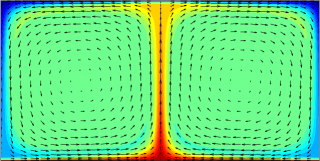
(b)
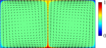
In addition to the turbulent convection generally observed at large Ra, there are much simpler steady solutions to the equations of motion such as the pair of steady counter-rotating rolls shown in figure 1. Steady coherent flows are not typically seen in large-Ra simulations or experiments because they are dynamically unstable. Nonetheless, they are part of the global attractor for the infinite-dimensional dynamical system defined by Rayleigh’s model, and recent results suggest that steady rolls may be one of the key coherent states comprising the ‘backbone’ of turbulent convection. In the case of no-slip top and bottom boundaries Waleffe et al. (2015) and Sondak et al. (2015) found that, over the range of Rayleigh numbers they explored, two-dimensional (2D) steady rolls display Nu values very close to those of three-dimensional (3D) convective turbulence, provided that the horizontal period of the rolls is tuned to maximize Nu at each value of Ra.
Here we report computations of steady 2D convective rolls in the case of stress-free top and bottom boundaries. We have carried out computations using spectral methods over eight orders of magnitude in Ra, four orders of magnitude in , and more than an order of magnitude in the aspect ratio , defined as the width-to-height ratio of a pair of rolls. As in the no-slip case, our steady states share many features with time-dependent simulations between stress-free boundaries (Paul et al., 2012; Wang et al., 2020). Moreover, the results verify predictions about the limit made by Chini & Cox (2009) who extended an approach initiated by Robinson (1967) to construct matched asymptotic approximations of steady rolls between stress-free boundaries. In particular, our computations agree quantitatively with the asymptotic prediction that uniformly in with a -dependent prefactor that assumes its maximum value at , and with corresponding asymptotic predictions about the Reynolds number that are derived in the Appendix. The rest of this paper is organized as follows. The equations governing Rayleigh–Bénard convection and our numerical scheme for computing steady solutions are outlined in § 2. The computational results are presented in § 3, followed by further discussion in § 4.
2 Governing equations and computational methods
The Boussinesq approximation to the Navier–Stokes equations used by Rayleigh (1916) to model convection in a 2D fluid layer are, in dimensionless variables,
| (1a) | ||||
| (1b) | ||||
| (1c) | ||||
where is the velocity, is the pressure, and is the temperature. The system has been nondimensionalized using the layer thickness , the thermal diffusion time , where is the thermal diffusivity, and the temperature drop from the bottom boundary to the top one.
The dimensionless spatial domain is , and all dependent variables are taken to be -periodic in . At the lower () and upper () boundaries, the temperature satisfies isothermal conditions while the velocity field satisfies no-penetration and stress-free boundary conditions:
| (2) |
The three dimensionless parameters of the problem are the aspect ratio , the Prandtl number , where is the kinematic viscosity, and the Rayleigh number , where is the gravitational acceleration vector and is the thermal expansion coefficient. A single pair of the steady rolls computed here fits in the domain, meaning the aspect ratio of the pair is while that of each individual roll is .
The static conduction state, for which and , solves 1 and 2 at all parameter values. Rayleigh (1916) showed that rolls vertically spanning the layer with aspect ratio bifurcate supercritically from the conduction state as Ra increases past
| (3) |
where is the wavenumber of the fundamental period of the domain. The conduction state is absolutely stable if for all admitted by the domain; see, e.g., Goluskin (2015).
The Nusselt number is defined as the ratio of total mean heat flux in the vertical direction to the flux from conduction alone:
| (4) |
where and are dimensionless solutions of 1 and indicates an average over space and infinite time. (For steady states the time average is not needed.) The governing equations imply the equivalent expressions
| (5) |
the latter of which self-evidently ensures for all sustained convection. Another emergent measure of the intensity of convection is the bulk Reynolds number defined using the dimensional root-mean-squared velocity , which in terms of dimensional quantities is . We choose our reference frame such that , so in dimensionless terms
| (6) |
We compute steady () solutions of 1 using a vorticity–stream function formulation,
| (7a) | ||||
| (7b) | ||||
| (7c) | ||||
where the stream function is defined by , the (negative) scalar vorticity is , and is the deviation of the temperature field from the conduction profile . The boundary conditions used in our computations are that , , and vanish on both boundaries. The latter two conditions follow from the stress-free and fixed-temperature conditions, respectively. Impenetrability of the boundaries implies that is constant on each boundary, and choosing the reference frame where requires these constants to be identical. Their value can be fixed to zero since translating by a constant does not affect the dynamics.
We solve the time-independent equations 7 numerically using a Newton–GMRES (generalised minimal residual) iterative scheme. Starting with an initial iterate that does not exactly solve 7, each iteration of the Newton’s method applies a correction until the resulting iterates have converged to a solution of 7. Following Wen et al. (2015b) and Wen & Chini (2018), the linear partial differential equations for the corrections are
| (8a) | ||||
| (8b) | ||||
| (8c) | ||||
where the superscript denotes the Newton iterate, the corrections are defined as
| (9) |
and vanish on the boundaries, and
| (10a) | ||||
| (10b) | ||||
| (10c) | ||||
are the residuals of the nonlinear steady equations 7. We simplify the implementation by setting , in which case can be obtained by solving for a given . After this simplification, the pair 8a and 8c can be solved simultaneously for and .
For each iteration of Newton’s method, we solve 8a and 8c iteratively using the GMRES method (Trefethen & Bau III, 1997). The spatial discretization is spectral, using a Fourier series in and a Chebyshev collocation method in (Trefethen, 2000). The operator is used as a preconditioner to accelerate convergence of the GMRES iterations. The roll states of interest have centro-reflection symmetries (cf. figure 1),
| (11) |
which allow the full fields to be recovered from their values on one quarter of the domain, so we encode these symmetries to reduce the number of unknowns. The GMRES iterations are stopped once the -norm of the relative residual of (8) is less than , and the Newton iterations are stopped once the -norm of the relative residual of (7) is less than . For Ra not far above the critical value , convergence to rolls of period is accomplished by choosing the initial iterate with and . For each , results from smaller Ra (or ) are used as the initial iterate for larger Ra (or ).
3 Results
We computed steady rolls over a wide range of Ra starting just above the value at which the rolls bifurcate from the conduction state and ranging up to or higher depending on the other parameters. Computations were carried out for and a range of values of such that the fundamental wavenumber lies in . Data for all the cases are tabulated in the Supplementary Material.
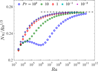
Our computations reach sufficiently large Ra to show clear asymptotic scalings of bulk quantities:
| (12) |
Both of these scalings are predicted by the asymptotic analysis of Chini & Cox (2009), although only the Nu scaling was stated explicitly there. Chini & Cox gave an asymptotic prediction for the prefactor but not for . Using their asymptotic approximations for the stream function and vorticity within each convection roll, we derived an expression for in terms of that is presented in the Appendix.
(a)
(b)
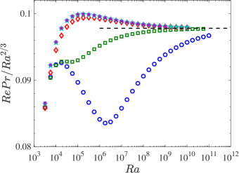
Figure 2 shows the Ra-dependence of the compensated quantities and for rolls of aspect ratio () at various . Rolls of this aspect ratio bifurcate from the conduction state at the Rayleigh number . It is clear from figure 2 that both Nu and the Péclet number become independent of as , as predicted by the asymptotics of Chini & Cox (2009), and also as Ra decreases towards the -independent value . Convergence to the large-Ra asymptotic scaling is slower when is larger, at least over the four decades of considered here. Numerical values of Nu and at large Ra suggest scaling prefactors that are indistinguishable from the values and predicted by asymptotic analysis.
(a)
(b)
(a)
(b)
(a)
(b)
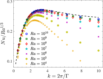
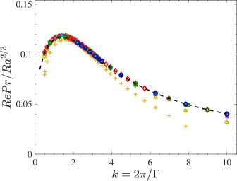
Nusselt and Reynolds numbers of steady rolls converge to the asymptotic scalings 12 over the full range for which we have computed steady rolls. This is evident in figure 3 where the -dependence of the compensated quantities and is shown for various Ra in the case. As Ra increases these quantities converge to asymptotic curves that we have called and . It is clear from the figure that this convergence is slower when is larger, and that reaches its asymptotic scaling sooner than Nu does. Since rolls with are the first to bifurcate from the conduction state, at , this is the that initially maximizes both Nu and . As , the values that maximize Nu and approach the asymptotic values () and (), respectively, where the corresponding maximal prefactors are and .
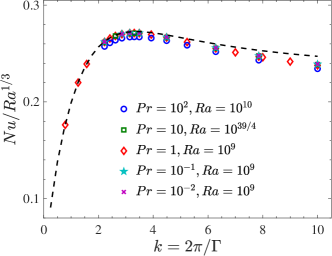
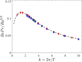
Both Nu and the Péclet number of steady rolls become nearly independent of as Ra grows large. The large-Ra coalescence of data for different is evident for the case in figure 2, as is the fact that can have a substantial effect in the pre-asymptotic regime. To show that -independence at large Ra occurs over the full range of our computations, figure 4 depicts the -dependence of compensated Nu and at large Ra for various . All and values plotted in figure 4 fall close to the asymptotic predictions for and that, at leading order in the asymptotic small parameter , are independent of .
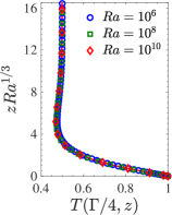
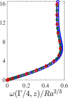
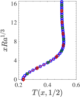
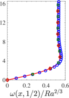
The asymptotic scaling of steady rolls at large Ra is reflected not only in the collapse of rescaled bulk quantities like and but also in the collapse of the boundary and internal layer profiles when the appropriate spatial variable is stretched by . Figure 5 shows this collapse of the temperature and vorticity profiles at the bottom boundary and at the left edge of the periodic domain for the case where and (). Coincidence of these scaled profiles at large Ra confirms that the thickness of both the thermal and vorticity layers scale like on all four edges of a single convection roll, while both fields are strongly homogenized in the interior with and . Profiles at other are not shown but collapse similarly. These findings confirm the deduction of a homogenized interior by Chini & Cox (2009), as well as their prediction that the core vorticity magnitude is asymptotic to uniformly in .
Another quantity of interest is the kinetic energy dissipation rate per unit mass,
| (13) |
where ∗ denotes dimensional variables. The corresponding bulk viscous dissipation coefficient can be expressed in dimensionless variables as
| (14) |
Identity 5 gives , so the asymptotic scalings 12 imply
| (15) |
That is, depends asymptotically on Ra and via the distinguished combination that is asymptotic to . This scaling of the dissipation coefficient is characteristic of flows without viscous boundary layers, such as laminar Couette or Poiseuille flow, consistent with the steady velocity fields computed here (cf. figure 1). Indeed, for stress-free steady convection, viscous dissipation is dominated by that in the homogenized core since the vorticity is of the same asymptotic magnitude in the core as in the thin vorticity layers.
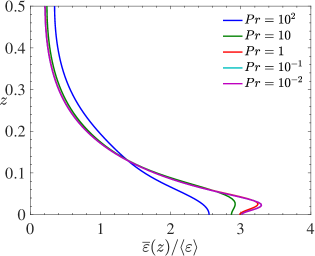
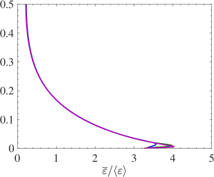
The average of dissipation over time and horizontal directions, denoted , has been used to compare convection between the cases of stress-free and no-slip boundaries. In 3D simulations of the stress-free case at , Petschel et al. (2013) found that the normalized profile exhibits ‘dissipation layers’ near the boundaries that depend strongly on . In steady rolls, on the other hand, we find that is independent of at asymptotically large Ra, as shown in figure S1 of the Supplementary Material.
4 Discussion
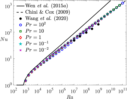
The steady rolls we have computed share many features with unsteady flows from DNS of Rayleigh–Bénard convection with isothermal stress-free boundary conditions. In recent simulations, Wang et al. (2020) found multistability between unsteady states exhibiting various numbers of roll pairs in wide 2D domains. Each of the coexisting states suggested scalings approaching the and asymptotic behaviour of steady rolls. As in the steady case, the prefactors of these scalings depended on the mean aspect ratios of the unsteady rolls. The highest Nusselt numbers among Wang et al.’s data occur in five-roll-pair states in a domain—meaning each roll pair has on average—but steady rolls have still larger Nu. At and , for example, the DNS exhibit and while steady rolls at the same parameters yield the larger values of and , and comparisons at other Ra are similar (cf. Table S4 of the Supplementary Material). Figure 6 shows the Nu of these five-roll-pair DNS states along with the larger Nu of the steady rolls computed here for various and . The steady rolls also achieve larger Nu values than have been attained in other unsteady simulations with stress-free boundaries in 2D (van der Poel et al., 2014; Goluskin et al., 2014) and in 3D (Petschel et al., 2013; Pandey et al., 2014; Pandey & Verma, 2016; Pandey et al., 2016).
Comparing steady rolls in the stress-free case with those previously computed in the no-slip case, there are significant differences in their dependence on the aspect ratio . With stress-free boundaries, for each as , with maximal asymptotic heat transport attained by rolls of optimal aspect ratio . In the no-slip computations of Waleffe et al. (2015) and Sondak et al. (2015), on the other hand, the values that maximize Nu decrease towards zero proportionally to at large Ra. (A similar phenomenon occurs in porous medium Rayleigh–Bénard convection; see Wen et al. (2015b).) The no-slip steady rolls display Nu scaling like when is fixed but scaling like when the optimal is chosen to maximize Nu at each Ra. The measured exponent 0.31 is unlikely to be exact, so it remains possible that the asymptotic scaling of optimal- steady rolls is in the no-slip case, as in the stress-free case.
Steady rolls in the stress-free and no-slip cases differ also in their dependence on the Prandtl number. Only with stress-free boundaries do the Nusselt number Nu and Péclet number apparently become uniform in as . To see how this -independence emerges in the stress-free scenario, first note that area-integrated work by the buoyancy forces must balance area-integrated viscous dissipation—i.e., in the dimensionless formulation of 4 and 5. The former integral is dominated by plumes since the roll’s core is isothermal, so it scales proportionally to the dimensional quantity , where is the dimensional plume thickness. The latter integral is dominated by the core since the vorticity is everywhere in the stress-free case, so this integral scales proportionally to the dimensional quantity . Balancing advection with diffusion of temperature anomalies in the thermal boundary layers, which also have thickness , requires that scale in proportion to . Combining this scaling relationship with that from the integral balance gives the dimensionless thermal boundary layer thickness as —and so —uniformly in . These relationships also imply that is proportional to , and so the Péclet number scales as uniformly in . Ultimately, it is the passivity of the vorticity boundary layers that results in the -independence of these emergent bulk quantities. The vorticity layers not only make no contribution to the total dissipation at leading order, they also have no leading-order effect on the stream function that is responsible for the convective flux .
The scaling found at large Ra for steady rolls and approximately evidenced in the DNS of Wang et al. (2020) means that buoyancy forces can sustain substantially faster-than-free-fall velocities. Indeed, if flow speeds were limited by the maximum buoyancy acceleration acting across the layer height then dimensional characteristic velocities could not be of larger order than , and could not be larger than . Such may be expected if the bulk flow were dominated by effectively independent rising and falling plumes. Significantly higher speeds apparently persist within coherent convection rolls, whether steady or unsteady.
Although steady rolls cannot give heat transport larger than as in the stress-free case (Chini & Cox, 2009), it is an open question whether larger Nu can result from time-dependent flows or other types of steady states in either 2D or 3D. Rigorous upper bounds on Nu derived from the governing equations—bounds depending on Ra that apply to all flows regardless of whether they are steady or unsteady and stable or unstable—do not rule out Nu growing faster than . Specifically, for the 2D stress-free case Whitehead & Doering (2011) proved analytically that uniformly in both and domain aspect ratio. Wen et al. (2015a) improved the prefactor of this bound by solving the relevant variational problem numerically, computing bounds up to large finite Ra with a prefactor depending weakly on . The numerical upper bound they computed for is shown in figure 6; its scaling at large Ra is . For 3D flows in the stress-free case only the larger upper bound has been proved (Doering & Constantin, 1996). It remains to be seen whether upper bounds smaller than or can be proved for 2D or 3D flows, respectively, and whether there exists any sequence of solutions for which Nu grows faster than . In view of available evidence it is possible that, at each Ra and , the steady 2D roll with the largest value of Nu—i.e., with Nu maximized over —transports more heat than any other 2D or 3D solution. We are aware of no counterexamples to this possibility, either in the stress-free case studied here or in the no-slip case.
Acknowledgements
We thank L.M. Smith, D. Sondak and F. Waleffe for helpful discussions. This research was supported in part by US National Science Foundation awards DMS-1515161 and DMS-1813003, Canadian NSERC Discovery Grants Program awards RGPIN-2018-04263, RGPAS-2018-522657 and DGECR-2018-00371, and computational resources and services provided by Advanced Research Computing at the University of Michigan.
Declaration of interests
The authors report no conflict of interest.
Appendix A Asymptotic calculation of
In this Appendix we derive the asymptotic scaling relation for that follows from the asymptotic analysis of Chini & Cox (2009) but is not reported there. In the large-Ra limit, a steady roll’s velocity field is properly scaled by rather than by the thermal diffusion velocity . Accordingly, we introduce the rescaled dimensionless velocity , which is related to the dimensionless velocity in 1 by . With this rescaling, the expression 6 for becomes
| (16) |
where is the correspondingly rescaled stream function. Consequently, the prefactor in the asymptotic relation 12 for satisfies
| (17) |
To evaluate the right-hand side of (17) in limit we first integrate by parts to find
| (18) |
where . The asymptotic approximation in (18) follows from two asymptotic estimates. First, the vorticity in a steady roll’s core is homogenized to a spatially uniform value as , and according to the analysis of Chini & Cox this value is related the prefactor in the – asymptotic relation via . Second, owing to the stress-free conditions and symmetries on a steady roll’s periphery, the vorticity field is of the same asymptotic order in both the vorticity boundary layers and the core, so the contribution of these boundary layers to the middle integral in (18) is negligible relative to that from the core where .
Unlike the temperature and vorticity fields, the stream function at leading order in is a smooth function over the entire spatial domain. The leading order expression for given by equations (22)–(23) of Chini & Cox is, in our notation,
| (19) |
Substituting 19 into the right-hand side of 18, integrating term-by-term, dividing by the cell width to obtain the spatial average, and taking the square root of the resulting expression gives the asymptotic prediction
| (20) |
Values of and corresponding values of for various are given in Table S1 of the Supplementary Material.
Supplementary Material
Table S1 gives numerical values of the asymptotic prefactors in expression (3.1) for the steady rolls constructed in the asymptotic analysis of Chini & Cox (2009). Tables S2 and S3 give the Nu and values plotted in figure 2. Table S4 compares steady rolls to unsteady rolls with the same mean aspect ratio from the DNS of Wang et al. (2020).
Figure S1 shows the normalized dissipation profiles of steady rolls at various for Ra values of and . There is much less variation with at the larger Ra value, reflecting the -independence that is predicted in the asymptotic limit. Only the profile is significantly different from the others when ; convergence to asymptotic behaviour as is slower at larger (cf. figure 1).
| 0.25 | 0.09084366 | 0.08479653 | 5.25 | 0.26516638 | 0.07042333 | |
| 0.5 | 0.13783563 | 0.10165665 | 5.5 | 0.26383550 | 0.06791123 | |
| 0.75 | 0.17242486 | 0.11048428 | 5.75 | 0.26253039 | 0.06554476 | |
| 1 | 0.19909232 | 0.11516486 | 6 | 0.26126222 | 0.06331554 | |
| 1.25 | 0.21981992 | 0.11716681 | 6.25 | 0.26003730 | 0.06121496 | |
| 1.5 | 0.23579393 | 0.11727251 | 6.5 | 0.25886080 | 0.05923472 | |
| 1.75 | 0.24788488 | 0.11600002 | 6.75 | 0.25773340 | 0.05736652 | |
| 2 | 0.25681088 | 0.11373790 | 7 | 0.25665667 | 0.05560274 | |
| 2.25 | 0.26318917 | 0.11079160 | 7.25 | 0.25563005 | 0.05393607 | |
| 2.5 | 0.26754979 | 0.10740171 | 7.5 | 0.25465196 | 0.05235964 | |
| 2.75 | 0.27033921 | 0.10375413 | 7.75 | 0.25372157 | 0.05086718 | |
| 3 | 0.27192661 | 0.09998906 | 8 | 0.25283657 | 0.04945277 | |
| 3.25 | 0.27260954 | 0.09620876 | 8.25 | 0.25199552 | 0.04811103 | |
| 3.5 | 0.27262477 | 0.09248559 | 8.5 | 0.25119483 | 0.04683679 | |
| 3.75 | 0.27215669 | 0.08886847 | 8.75 | 0.25043350 | 0.04562556 | |
| 4 | 0.27134834 | 0.08538889 | 9 | 0.24970964 | 0.04447307 | |
| 4.25 | 0.27030747 | 0.08206516 | 9.25 | 0.24902004 | 0.04337532 | |
| 4.5 | 0.26911578 | 0.07890636 | 9.5 | 0.24836456 | 0.04232885 | |
| 4.75 | 0.26783386 | 0.07591494 | 9.75 | 0.24773960 | 0.04133018 | |
| 5 | 0.26650668 | 0.07308893 | 10 | 0.24714363 | 0.04037628 |
| 1.46630 | 1.46614 | 1.46687 | 1.46716 | 1.46718 | ||
| 2.37255 | 2.37025 | 2.36637 | 2.37324 | 2.37425 | ||
| 3.18564 | 3.18049 | 3.15193 | 3.16265 | 3.16748 | ||
| 4.05203 | 4.04468 | 3.98471 | 3.96052 | 3.97220 | ||
| 5.07914 | 5.07051 | 4.98831 | 4.86435 | 4.88129 | ||
| 6.32515 | 6.31587 | 6.22172 | 5.94155 | 5.94945 | ||
| 7.83124 | 7.82158 | 7.72035 | 7.25591 | 7.21592 | ||
| 9.65227 | 9.64234 | 9.53590 | 8.89159 | 8.72489 | ||
| 11.8568 | 11.8467 | 11.7360 | 10.9457 | 10.5267 | ||
| 14.5268 | 14.5164 | 14.4021 | 13.5059 | 12.6816 | ||
| 17.7612 | 17.7506 | 17.6329 | 16.6557 | 15.2701 | ||
| 21.6798 | 21.6690 | 21.5483 | 20.5044 | 18.4060 | ||
| 26.4274 | 26.4164 | 26.2929 | 25.1935 | 22.2598 | ||
| 32.1797 | 32.1685 | 32.0425 | 30.8962 | 27.0879 | ||
| 39.1494 | 39.1379 | 39.0094 | 37.8234 | 33.2279 | ||
| 47.5938 | 47.5822 | 47.4514 | 46.2312 | 41.0104 | ||
| 57.8250 | 57.8132 | 57.6802 | 56.4307 | 50.7115 | ||
| 70.2211 | 70.2091 | 70.0740 | 68.7989 | 62.6608 | ||
| 85.2397 | 85.2277 | 85.0905 | 83.7928 | 77.2962 | ||
| 103.437 | 103.424 | 103.285 | 101.967 | 95.1593 | ||
| 125.484 | 125.472 | 125.330 | 123.991 | 116.909 | ||
| 152.192 | 152.179 | 152.036 | 150.683 | 143.355 | ||
| 184.554 | 184.541 | 184.394 | 183.026 | 175.477 | ||
| 223.758 | 223.745 | 223.599 | 222.215 | 214.465 | ||
| 271.266 | 271.253 | 271.105 | 269.698 | 261.773 | ||
| 328.798 | 328.713 | 327.238 | 319.134 | |||
| 398.523 | 398.427 | 397.003 | 388.734 | |||
| 483.062 | 482.910 | 481.470 | 473.049 | |||
| 585.437 | 585.285 | 583.841 | 575.311 | |||
| 707.958 | 699.254 | |||||
| 858.111 | 849.325 | |||||
| 1040.21 | 1031.35 | |||||
| 1251.98 |
| 4.860211 | 4.859365 | 4.863013 | 4.864534 | 4.864669 | ||
| 11.11289 | 11.10342 | 11.08274 | 11.10817 | 11.11225 | ||
| 18.64998 | 18.62765 | 18.48547 | 18.50202 | 18.52133 | ||
| 29.18438 | 29.14861 | 28.81749 | 28.56985 | 28.61439 | ||
| 44.44510 | 44.39718 | 43.87005 | 42.81088 | 42.85149 | ||
| 66.65392 | 66.59490 | 65.87916 | 63.22068 | 63.10225 | ||
| 99.00479 | 98.93476 | 98.02324 | 92.79036 | 92.04534 | ||
| 146.2211 | 146.1395 | 145.0123 | 136.1512 | 133.5699 | ||
| 215.2057 | 215.1114 | 213.7389 | 200.3372 | 193.1899 | ||
| 316.0649 | 315.9563 | 314.2983 | 295.6302 | 278.8445 | ||
| 463.6093 | 463.4841 | 461.4878 | 436.6766 | 402.1873 | ||
| 679.5490 | 679.4041 | 677.0022 | 644.8536 | 580.6680 | ||
| 995.7158 | 995.5474 | 992.6546 | 951.6627 | 841.1621 | ||
| 1458.790 | 1458.594 | 1455.104 | 1403.377 | 1226.322 | ||
| 2137.241 | 2137.009 | 2132.789 | 2067.960 | 1803.793 | ||
| 3131.499 | 3131.224 | 3126.109 | 3045.229 | 2674.566 | ||
| 4588.895 | 4588.574 | 4582.361 | 4481.765 | 3981.512 | ||
| 6725.606 | 6725.221 | 6717.660 | 6592.805 | 5932.137 | ||
| 9858.786 | 9858.334 | 9849.112 | 9694.374 | 8833.901 | ||
| 14453.85 | 14453.31 | 14442.05 | 14250.46 | 13140.24 | ||
| 21193.84 | 21193.21 | 21179.44 | 20942.25 | 19519.46 | ||
| 31080.45 | 31079.68 | 31062.85 | 30769.81 | 28954.88 | ||
| 45585.16 | 45584.26 | 45563.33 | 45201.19 | 42895.45 | ||
| 66865.43 | 66864.32 | 66839.10 | 66391.72 | 63471.97 | ||
| 98091.13 | 98089.85 | 98058.98 | 97504.78 | 93819.57 | ||
| 143906.3 | 143882.5 | 143186.5 | 138542.0 | |||
| 211139.3 | 211107.6 | 210266.2 | 204428.0 | |||
| 309825.2 | 309769.0 | 308731.1 | 301407.4 | |||
| 454641.9 | 454573.4 | 453293.9 | 444122.9 | |||
| 665545.3 | 654078.8 | |||||
| 977028.2 | 962715.7 | |||||
| 1434327 | 1416484 | |||||
| 2083475 |
| Steady roll | DNS | |||||
|---|---|---|---|---|---|---|
| 53.2089 | 515.276 | 48.53 | 488.77 | |||
| 77.5286 | 1080.31 | 69.43 | 1016.46 | |||
| 116.711 | 2425.10 | 96.81 | 2202.08 | |||
| 169.146 | 5063.63 | 134.00 | 4552.41 | |||
| 253.606 | 11332.6 | 198.01 | 10135.1 | |||
[figure]style=plain,subcapbesideposition=top
(a)
(b)
References
- Chillà & Schumacher (2012) Chillà, Francesca & Schumacher, Joerg 2012 New perspectives in turbulent Rayleigh-Bénard convection. The European Physical Journal E 35 (7), 1–25.
- Chini & Cox (2009) Chini, G.P. & Cox, S.M. 2009 Large Rayleigh number thermal convection: Heat flux predictions and strongly nonlinear solutions. Physics of Fluids 21, 083603.
- Doering (2020) Doering, C.R. 2020 Turning up the heat in turbulent thermal convection. Proceedings of the National Academy of Sciences 117, 9671–9673.
- Doering & Constantin (1996) Doering, C. R. & Constantin, P. 1996 Variational bounds on energy dissipation in incompressible flows. III. Convection. Phys. Rev. E 53, 5957–5981.
- Goluskin (2015) Goluskin, D. 2015 Internally heated convection and Rayleigh–Bénard convection. Springer.
- Goluskin et al. (2014) Goluskin, D., Johnston, H., Flierl, G.R. & Spiegel, E.A. 2014 Convectively driven shear and decreased heat flux. Journal of Fluid Mechanics 759, 360–385.
- Kadanoff (2001) Kadanoff, L.P. 2001 Turbulent heat flow: Structures and scaling. Physics Today 54, 34–39.
- Lorenz (1963) Lorenz, E.N. 1963 Deterministic nonperiodic flow. Journal of the Atmospheric Sciences 20, 130–141.
- Malkus & Veronis (1958) Malkus, W.V.R. & Veronis, G. 1958 Finite amplitude cellular convection. Journal of Fluid Mechanics 4, 225–260.
- Newell & Whitehead (1969) Newell, A.C. & Whitehead, J.A. 1969 Finite bandwidth, finite amplitude convection. Journal of Fluid Mechanics 38, 279–303.
- Pandey et al. (2014) Pandey, A., Verma, M.K. & Mishra, P.K. 2014 Scaling of heat flux and energy spectrum for very large Prandtl number convection. Physical Review E 89, 023006.
- Pandey & Verma (2016) Pandey, A. & Verma, M. K. 2016 Scaling of large-scale quantities in Rayleigh–Bénard convection. Physics of Fluids 28, 095105.
- Pandey et al. (2016) Pandey, A., Verma, M. K., Chatterjee, A. G. & Dutta, B. 2016 Similarities between 2D and 3D convection for large Prandtl number. Pramana – J. Phys. 87, 13.
- Paul et al. (2012) Paul, S., Verma, M. K., Wahi, P., Reddy, S. K. & Kumar, K. 2012 Bifurcation analysis of the flow patterns in two-dimensional Rayleigh–Bénard convection. Int. J. Bifurc. Chaos 22, 1230018.
- Petschel et al. (2013) Petschel, K., Stellmach, S., Wilczek, M., Lülff, J. & Hansen, U. 2013 Dissipation layers in Rayleigh–Bénard convection: A unifying view. Physical Review Letters 110, 114502.
- van der Poel et al. (2014) van der Poel, E.P., Ostilla-Mónico, R., Verzicco, R. & Lohse, D. 2014 Effect of velocity boundary conditions on the heat transfer and flow topology in two-dimensional Rayleigh–Bénard convection. Physical Review E 90, 013017.
- Rayleigh (1916) Rayleigh, Lord 1916 On convection currents in a horizontal layer of fluid, when the higher temperature is on the under side. Philosophical Magazine 32, 529–546.
- Robinson (1967) Robinson, J.L. 1967 Finite amplitude convection cells. Journal of Fluid Mechanics 30, 577–600.
- Sondak et al. (2015) Sondak, D., Smith, L.M. & Waleffe, F. 2015 Optimal heat transport solutions for Rayleigh–Bénard convection. Journal of Fluid Mechanics 784, 565–595.
- Trefethen (2000) Trefethen, L.N. 2000 Spectral Methods in MATLAB. SIAM.
- Trefethen & Bau III (1997) Trefethen, L.N. & Bau III, D. 1997 Numerical Linear Algebra. Philadelphia: SIAM.
- Waleffe et al. (2015) Waleffe, F., Boonkasame, A. & Smith, L.M. 2015 Heat transport by coherent Rayleigh–Bénard convection. Physics of Fluids 27, 051702.
- Wang et al. (2020) Wang, Q., Chong, K.-L., Stevens, R.J.A.M., Verzicco, R. & Lohse, D. 2020 From zonal flow to convection rolls in Rayleigh–Bénard convection with free-slip plates. arXiv:2005.02084 .
- Wen & Chini (2018) Wen, B. & Chini, G.P. 2018 Inclined porous medium convection at large Rayleigh number. Journal of Fluid Mechanics 837, 670–702.
- Wen et al. (2015a) Wen, B., Chini, G.P., Kerswell, R.R. & Doering, C.R. 2015a Time-stepping approach for solving upper-bound problems: Application to two-dimensional Rayleigh–Bénard convection. Physical Review E 92, 043012.
- Wen et al. (2015b) Wen, B., Corson, L.T. & Chini, G.P. 2015b Structure and stability of steady porous medium convection at large Rayleigh number. Journal of Fluid Mechanics 772, 197–224.
- Whitehead & Doering (2011) Whitehead, J.P. & Doering, C.R. 2011 Ultimate state of two-dimensional Rayleigh–Bénard convection between free-slip fixed-temperature boundaries. Physical Review Letters 106, 244501.