This paper was converted on www.awesomepapers.org from LaTeX by an anonymous user.
Want to know more? Visit the Converter page.

Statistical inference for mean-field queueing systems

Ioannis Lambadaris, Ahmed Sid-Ali, Wei Sun , Yiqiang Q. Zhao
Department of Systems and Computer Engineering, Carleton University, Ottawa, Ontario, Canada. [email protected] of Mathematics and Statistics, Carleton University, Ottawa, Ontario, Canada. [email protected] of Mathematics and Statistics, Concordia University, Montreal, Canada. [email protected] of Mathematics and Statistics, Carleton University, Ottawa, Ontario, Canada. [email protected]
Abstract

Mean-field limits have been used now as a standard tool in approximations, including for networks with a large number of nodes. Statistical inference on mean-filed models has attracted more attention recently mainly due to the rapid emergence of data-driven systems. However, studies reported in the literature have been mainly limited to continuous models. In this paper, we initiate a study of statistical inference on discrete mean-field models (or jump processes) in terms of a well-known and extensively studied model, known as the power-of-LL (L2L\geq 2), or the supermarket model, to demonstrate how to deal with new challenges in discrete models. We focus on system parameter estimation based on the observations of system states at discrete time epochs over a finite period. We show that by harnessing the weak convergence results developed for the supermarket model in the literature, an asymptotic inference scheme based on an approximate least squares estimation can be obtained from the mean-field limiting equation. Also, by leveraging the law of large numbers alongside the central limit theorem, the consistency of the estimator and its asymptotic normality can be established when the number of servers and the number of observations go to infinity. Moreover, numerical results for the power-of-two model are provided to show the efficiency and accuracy of the proposed estimator.

2020 Mathematics Subject Classification: 60K2560K25 60K3560K35 62F1062F10 62F1262F12 Keywords: Mean-field; Queuing systems; Supermarket model; Least square estimation; Consistency; Asymptotic normality

1 Introduction

The origins of mean-field theory trace back to the pioneering works of Curie [8] and Weiss [36] in magnetism and phase transitions. Since then, this theory has expanded across a wide array of fields to study interacting particle systems, including statistical physics [9, 16, 23, 24], biological systems [10, 30], communication networks [4, 20, 21, 22], and mathematical finance [19, 27].

Moreover, the application of mean-field theory in queueing systems is traced back to the work of Dobrushin and Sukhov [14] and has since proliferated due to its many benefits, see, e.g., [11, 12, 31, 35] for further developments. Indeed, in stochastic service systems, particularly those involving multiple parallel queues, load balancing is commonly applied to enhance performance by shortening queues, reducing wait times, and increasing throughput. This balancing mechanism effectively modifies the input-output dynamics to improve the system’s quality of service. When such systems are viewed as interacting systems, mean-field theory becomes a natural framework to study their behavior. By using mean-field analysis, the performance of large systems can be evaluated by examining their limiting behavior as the system size approaches infinity. In particular, the limit often reduces when solving a deterministic system known as the mean-field limit, which corresponds to a McKean-Vlasov-type stochastic differential equation (SDE) solution. In McKean-Vlasov SDEs, the coefficients depend on both the process itself and its distribution, forming a class of non-linear SDEs. The study of such equations was initiated by McKean [23], inspired by Kac’s work in kinetic theory [25].

Although extensive literature exists on mean-field interacting systems, research on their statistical inference has only gained attention in recent years. The pioneering work in this area is Kasonga’s seminal paper [26], which addressed parameter estimation for interacting particle systems modeled by Itô SDEs through a maximum likelihood approach. After Kasonga’s work, interest in the topic waned for nearly two decades before reemerging with significant contributions, as seen in [1, 3, 5, 17, 29, 32] and references therein. Since then, the field has grown steadily, establishing itself as a crucial area of research. This renewed interest can be attributed to novel applications of mean-field theory and the rise of new technologies enabling access to massive datasets generated by systems of interacting agents.

To date, most statistical inference studies on mean-field models, such as those mentioned above, focus on interacting diffusion systems, with limited research on statistical inference for mean-field systems with jumps. Notable exceptions include [13] and [28], where the authors proposed asymptotic estimation for the Bernoulli interaction parameter in a system of interacting Hawkes processes as both the number of particles and time approach infinity. In particular, as discussed in [37], statistical inference in mean-field queueing models remains largely unexplored, despite statistical inference in queueing systems being an active area of research. The reader can consult for example [2] where a comprehensive survey on parameter and state estimation for queueing systems across various estimation paradigms was provided, yet it does not address statistical inference for mean-field queueing systems. To fill this gap, we propose in the current paper a statistical inference scheme for the parameters governing a specific mean-field queuing system, namely the supermarket model, also known as the power of L2L\geq 2 choices. Thus, to the best of our knowledge, our current proposal represents a novel contribution in this area.

The supermarket model was independently introduced by Vvedenskaya et al. [35] and Mitzenmacher [31]. It represents a system of NN parallel identical queues, each served by a single server with a service rate ν\nu and infinite buffer capacity. Tasks arrive at a rate of NλN\lambda; each task is allocated LL queues chosen uniformly at random among the NN and joins the shortest one, with ties resolved uniformly. All events in this system are independent. In particular, [35] and [31] studied the asymptotic behavior of the system as the number of servers becomes large, showing that the process associated with queue lengths converges to a deterministic limit represented by an infinite system of ordinary differential equations (ODEs). This model and its extensions have since become widely studied due to its theoretical and practical importance; see, e.g., [20, 6, 7] and the references therein. However, as noted, the statistical inference for this model remains unexplored, which is the focus of this paper.

We propose a statistical inference scheme to estimate the arrival and service rates in a supermarket model based on aggregate data obtained from discrete observations of a moment of the system over a finite period. To this end, we propose to exploit the ODE obtained at the mean-field limit to construct an approximate least square estimator (LSE). Then, using the law of large numbers and the central limit theorem established in the literature, we show that the proposed estimator is consistent and asymptotically normal as the number of servers and observations grows large. In addition, we test our estimator on synthetic data obtained by simulation which shows the accuracy of our approach.

It is worthwhile to provide the following remark: An intriguing general approach to statistical inference for mean-field systems was proposed in [18]. This approach leverages a “misspecified” or limiting model, created by approximating the system through large-systems asymptotics, incorporating the law of large numbers and central limit theorem. This enables constructing an approximate likelihood function, evaluated against the data generated by the true model. The estimator is then obtained by maximizing this approximate likelihood function. A key advantage of this method is that the approximate likelihood has a conditionally Gaussian structure, due to the central limit theorem, which allows for efficient numerical evaluation of the estimator. Although one might consider using a similar method to estimate parameters for the supermarket model, the complexity of the approximate likelihood for this model complicates the analysis of the estimator’s asymptotic properties. This difficulty motivates the adoption of an alternative approach, specifically, an approximate LSE scheme.

The rest of the paper is organized as follows: First, in Section 2, we recall the supermarket model and introduce the appropriate notations. We also review some well-known asymptotic results about the model, including a new technical result in Proposition 2.1 that will be used in the sequel. In Section 3, we introduce the inference scheme along with our LSE and prove both the consistency and asymptotic normality of the estimator. To facilitate the reading, we put all the long proofs in the appendices. Section 4 provides simulations demonstrating that our estimator accurately predicts the system parameters and validates the asymptotic normality result. Finally, in Section 5, we present conclusions and open questions, followed by the bibliography.

2 Queuing network with selection of the shortest queue among several servers

2.1 The setting

We start by recalling the supermarket model, first introduced separately in [31] and [35]. Consider a network with NN identical queues, each with a single server of service rate ν\nu and an infinite buffer. Tasks arrive at rate NλN\lambda, and each task is allocated LL queues with uniform probability among the NN servers and elects to join the shortest one, ties being resolved uniformly. The LL selected queues may coincide. All these random events are independent. Let XiN(t)X^{N}_{i}(t) denote the length of the ii-th queue at time tt and define the empirical measure process

ϱjN(t):=1Ni=1N𝟙{XiN(t)=j},j=0,1,,\displaystyle\varrho^{N}_{j}(t):=\frac{1}{N}\sum_{i=1}^{N}\mathds{1}_{\{X_{i}^{N}(t)=j\}},\quad j=0,1,\ldots,

which takes values in the space 𝒫(+)\mathcal{P}(\mathbb{Z}_{+}) of probability measures on +={0,1,2,}\mathbb{Z}_{+}=\{0,1,2,\dots\} identified with the infinite-dimensional simplex

𝒮:={s={sj}j+++:j=0sj=1},\displaystyle\mathcal{S}:=\bigg{\{}s=\{s_{j}\}_{j\in\mathbb{Z}_{+}}\in\mathbb{R}^{\mathbb{Z}_{+}}_{+}:\sum_{j=0}^{\infty}s_{j}=1\bigg{\}},

where +\mathbb{R}_{+} is the set of all non-negative real numbers. Define the subspace 𝒮N:=𝒮++N\mathcal{S}^{N}:=\mathcal{S}\cap\frac{\mathbb{Z}_{+}^{\mathbb{Z}_{+}}}{N}. Thus, ϱN(t)𝒮N\varrho^{N}(t)\in\mathcal{S}^{N} for all t0t\geq 0. Throughout this paper, we fix a constant T>0T>0. Let 𝒟([0,T],𝒮)\mathcal{D}([0,T],\mathcal{S}) be the Skorokhod space of càdlàg functions defined on [0,T][0,T] with values in 𝒮\mathcal{S}, equipped with the usual Skorokhod topology. Let 𝒞([0,T],𝒮)\mathcal{C}([0,T],\mathcal{S}) be the space of continuous functions defined on [0,T][0,T] with values on 𝒮\mathcal{S}, equipped with the uniform topology.

2.2 Law of large numbers and central limit theorem for the empirical process

We recall now some results describing the asymptotic behavior of the supermarket model that will be used to build the statistical inference scheme and the related analysis. For p1p\geq 1, denote by p\ell_{p} the space of pp-th summable sequences, i.e.,

p={x={xj}j++:j=0|xj|p<},\displaystyle\ell_{p}=\bigg{\{}x=\{x_{j}\}_{j\in\mathbb{Z}_{+}}\in\mathbb{R}^{\mathbb{Z}_{+}}:\sum_{j=0}^{\infty}|x_{j}|^{p}<\infty\bigg{\}},

and denote by p\|\cdot\|_{p} the norm on it. In particular, let 2\ell_{2} be the space of square summable sequences equipped with the inner product

x,y=j=0xjyj,\ \langle x,y\rangle=\sum_{j=0}^{\infty}x_{j}y_{j},

which makes it a Hilbert space. Moreover, define its subspace

~2:={s2:j=0j2sj2<,j=0sj=0}.\displaystyle\tilde{\ell}_{2}:=\bigg{\{}s\in\ell_{2}:\sum_{j=0}^{\infty}j^{2}s_{j}^{2}<\infty,\,\sum_{j=0}^{\infty}s_{j}=0\bigg{\}}.

Furthermore, for any j+j\in\mathbb{Z}_{+}, denote by ej2e_{j}\in\ell_{2} the vector with 1 at the jj-th coordinate and 0 elsewhere.

We first state the law of large numbers established in [20, Theorem 3.4] and reformulated in [6, Corollary 1].

Theorem 2.1

Suppose that ϱN(0)ϱ0\varrho^{N}(0)\rightarrow\varrho_{0} in 𝒮\mathcal{S} as NN\rightarrow\infty. Then ϱNϱ\varrho^{N}\rightarrow\varrho in probability in 𝒟([0,T],𝒮)\mathcal{D}([0,T],\mathcal{S}), where ϱ\varrho is the unique solution in 𝒞([0,T],𝒮)\mathcal{C}([0,T],\mathcal{S}) to the ODE:

ϱ˙(t)=F(ϱ(t)),ϱ(0)=ϱ0,\displaystyle\dot{\varrho}(t)=F(\varrho(t)),\quad\varrho(0)=\varrho_{0}, (2.1)

and, for any x1x\in\ell_{1},

F(x)\displaystyle F(x) =\displaystyle= λj=0[i=1L(Li)xj1i(m=jxm)Lii=1L(Li)xji(m=j+1xm)Li]ej\displaystyle\lambda\sum_{j=0}^{\infty}\bigg{[}\sum_{i=1}^{L}{L\choose i}x^{i}_{j-1}\bigg{(}\sum_{m=j}^{\infty}x_{m}\bigg{)}^{L-i}-\sum_{i=1}^{L}{L\choose i}x_{j}^{i}\bigg{(}\sum_{m=j+1}^{\infty}x_{m}\bigg{)}^{L-i}\bigg{]}e_{j} (2.2)
+νj=0[xj+1xj]ej.\displaystyle+\nu\sum_{j=0}^{\infty}[x_{j+1}-x_{j}]e_{j}.

Next, we state results about the fluctuations of the empirical measure process ϱN\varrho^{N} from its law of large number limit ϱ\varrho. To this end, define the process

𝒵N(t):=N(ϱN(t)ϱ(t)),t[0,T],\displaystyle\mathcal{Z}^{N}(t):=\sqrt{N}(\varrho^{N}(t)-\varrho(t)),\quad t\in[0,T],

the operator

Φ(t)\displaystyle\Phi(t) :=\displaystyle:= λj=0(ej+1ej)(ej+1ej)T(i=1L(Li)[ϱj(t)]i(m=j+1ϱm(t))Li)\displaystyle\lambda\sum_{j=0}^{\infty}(e_{j+1}-e_{j})(e_{j+1}-e_{j})^{T}\bigg{(}\sum_{i=1}^{L}{L\choose i}[\varrho_{j}(t)]^{i}\bigg{(}\sum_{m=j+1}^{\infty}\varrho_{m}(t)\bigg{)}^{L-i}\bigg{)} (2.3)
+νj=1(ej1ej)(ej1ej)Tϱj(t),\displaystyle+\nu\sum_{j=1}^{\infty}(e_{j-1}-e_{j})(e_{j-1}-e_{j})^{T}\varrho_{j}(t),

and the map G:~2×𝒮~2G:\tilde{\ell}_{2}\times\mathcal{S}\rightarrow\tilde{\ell}_{2} by

Gj(x,s):=uFj(s+ux)|u=0,j+,x~2,s𝒮.\displaystyle G_{j}(x,s):=\frac{\partial}{\partial u}F_{j}(s+ux)\bigg{|}_{u=0},\quad j\in\mathbb{Z}_{+},x\in\tilde{\ell}_{2},s\in\mathcal{S}. (2.4)

Finally, we recall the definition of cylindrical Brownian motion which is a generalization of the scalar Brownian motion to Hilbert spaces.

Definition 2.1

A collection of continuous real-valued stochastic processes {(Wt(h))0tT:h2}\{(W_{t}(h))_{0\leq t\leq T}:h\in\ell_{2}\} defined on a filtered probability space (Ω,,,{t})(\Omega,\mathcal{F},\mathbb{P},\{\mathcal{F}_{t}\}) is called an 2\ell_{2}-cylindrical Brownian motion if, for every h2h\in\ell_{2}, (Wt(h))0tT(W_{t}(h))_{0\leq t\leq T} is an {t}\{\mathcal{F}_{t}\}-Brownian motion with variance th22t\|h\|^{2}_{2} and, for all h,k2h,k\in\ell_{2},

W(h),W(k)t=th,k2,t[0,T].\displaystyle\langle W(h),W(k)\rangle_{t}=t\langle h,k\rangle_{2},\quad t\in[0,T].

We state now the central limit theorem introduced in [6, Theorem 2].

Theorem 2.2

Suppose that supNj=0j2ϱjN(0)<\sup_{N\in\mathbb{N}}\sum_{j=0}^{\infty}j^{2}\varrho^{N}_{j}(0)<\infty and ϱN(0)ϱ0\varrho^{N}(0)\rightarrow\varrho_{0} in 𝒮\mathcal{S} as NN\rightarrow\infty. Also, suppose that 𝒵N(0)z0\mathcal{Z}^{N}(0)\rightarrow z_{0} in 2\ell_{2} and that

supNj=0j2(𝒵jN(0))2<.\displaystyle\sup_{N\in\mathbb{N}}\sum_{j=0}^{\infty}j^{2}(\mathcal{Z}^{N}_{j}(0))^{2}<\infty.

Then 𝒵N\mathcal{Z}^{N} converges to 𝒵\mathcal{Z} in distribution in 𝒟([0,T],2)\mathcal{D}([0,T],\ell_{2}) as NN\rightarrow\infty, where 𝒵\mathcal{Z} is the unique weak solution to the following SDE:

d𝒵(t)=G(𝒵(t),ϱ(t))dt+a(t)dW(t),𝒵(0)=z0~2,\displaystyle d\mathcal{Z}(t)=G(\mathcal{Z}(t),\varrho(t))dt+a(t)dW(t),\quad\mathcal{Z}(0)=z_{0}\in\tilde{\ell}_{2}, (2.5)

GG is defined by (2.4)(\ref{G-map}), a(t)a(t) is the symmetric square root of the operator Φ(t)\Phi(t) in (2.3)(\ref{Phi-op}), i.e., a2(t)=Φ(t)a^{2}(t)=\Phi(t), and WW is an 2\ell_{2}-cylindrical Brownian motion.

Remark 1

The stochastic integral 0ta(s)𝑑W(s)\int_{0}^{t}a(s)dW(s) represents an 2\ell_{2}-valued Gausssian martingale M(t)M(t) given as

Mi(t)=j=00tAij(s)𝑑Bj(s),t[0,T],i+,\displaystyle M_{i}(t)=\sum_{j=0}^{\infty}\int_{0}^{t}A_{ij}(s)dB_{j}(s),\quad t\in[0,T],i\in\mathbb{Z}_{+}, (2.6)

with Aij(s)=ei,a(s)ej2A_{ij}(s)=\langle e_{i},a(s)e_{j}\rangle_{2} and {Bj}j+\{B_{j}\}_{j\in\mathbb{Z}_{+}} is an independent sequence of standard Brownian motions. The well-posedness of the SDE (2.5) was established in [6, Proposition 2].

2.3 The power of two choices model

For the sake of simplicity, we focus in this paper on a special case of the supermarket model obtained when L=2L=2. This model, known as the power of two choices, was first introduced and analyzed in [31]. In this case, the operator FF in (2.2)(\ref{F-L-op}) takes the following explicit form:

F(x)=λj=0[2xj1m=jxm2xjm=j+1xm+xj12xj2]ej+νj=0[xj+1xj]ej,x1,\displaystyle F(x)=\lambda\sum_{j=0}^{\infty}\bigg{[}2x_{j-1}\sum_{m=j}^{\infty}x_{m}-2x_{j}\sum_{m=j+1}^{\infty}x_{m}+x^{2}_{j-1}-x_{j}^{2}\bigg{]}e_{j}+\nu\sum_{j=0}^{\infty}[x_{j+1}-x_{j}]e_{j},\quad x\in\ell_{1}, (2.7)

the map G:~2×𝒮2G:\tilde{\ell}_{2}\times\mathcal{S}\rightarrow{\ell}_{2} in (2.4)(\ref{G-map}) takes now the explicit form:

Gj(x,s)=2λm=j[xj1sm+sj1xmxjsm+1sjxm+1]+ν(xj+1xj),j+,x~2,s𝒮,\displaystyle G_{j}(x,s)=2\lambda\sum_{m=j}^{\infty}[x_{{j}-1}s_{m}+s_{{j}-1}x_{m}-x_{j}s_{m+1}-s_{j}x_{m+1}]+\nu(x_{{j}+1}-x_{j}),\quad j\in\mathbb{Z}_{+},x\in\tilde{\ell}_{2},s\in\mathcal{S},

and for any t[0,T]t\in[0,T], the operator Φ(t)\Phi(t) in (2.3)(\ref{Phi-op}) becomes

Φ(t)\displaystyle\Phi(t) =\displaystyle= λj=0(ej+1ej)(ej+1ej)T(2ϱj(t)m=j+1ϱm(t)+[ϱj(t)]2)\displaystyle\lambda\sum_{j=0}^{\infty}(e_{j+1}-e_{j})(e_{j+1}-e_{j})^{T}\bigg{(}2\varrho_{j}(t)\sum_{m=j+1}^{\infty}\varrho_{m}(t)+[\varrho_{j}(t)]^{2}\bigg{)}
+νj=1(ej1ej)(ej1ej)Tϱj(t).\displaystyle+\nu\sum_{j=1}^{\infty}(e_{j-1}-e_{j})(e_{j-1}-e_{j})^{T}\varrho_{j}(t).

The following result shows that the solution to (2.5)(\ref{CLT-Budhi-eqn}) is a Gaussian process. Although the proof is given for the power of two choices model, it can be adapted to cover the case with general L2L\geq 2.

Proposition 2.1

Suppose that L = 2. Then, the solution 𝒵(t)\mathcal{Z}(t) to the SDE (2.5)(\ref{CLT-Budhi-eqn}) is a Gaussian process.

Proof

See Appendix A. \Box

3 Statistical inference of the supermarket model

Suppose the service and arrival rates, ν\nu and λ\lambda, that govern the system are unknown. Our goal is to estimate these parameters using observations collected over a specific time interval [0,T][0,T]. The complexity of the system’s dynamics makes brute-force Monte Carlo estimation computationally intensive, particularly as the number of nodes, NN, increases. Therefore, we propose developing an estimator that utilizes the weak convergence results outlined in Section 2, specifically the law of large numbers presented in Theorem 2.1 and the central limit theorem in Theorem 2.2.

In particular, we construct an approximate LSE based on the ODE given in (2.1)(\ref{ODE-LLN-Budhi}). We subsequently demonstrate that this estimator is consistent and asymptotically normal as both the system size and the number of observations tend to infinity. For convenience, we denote the vector of unknown parameters as θ=(λ,ν)\theta=(\lambda,\nu).

3.1 The data

Our objective is to estimate the parameter vector θ\theta that governs the dynamics of the power-of-two model based on observations collected over a finite time interval. Specifically, we assume that observations are not available for every server in the network; instead, they are gathered as an aggregate measure of the system. Collecting individual data for each server can be prohibitively costly in practice, particularly for large networks, which justifies our approach to data collection.

In this context, we assume that the available data for inference includes observations of the empirical measure of the system, ϱN(t)\varrho^{N}(t), over the finite time interval [0,T][0,T] at mm discrete points, defined as tk=kTmt_{k}=\frac{kT}{m}:

ϱjN(tk):=1Ni=1N𝟙{XiN(tk)=j},j+,k=1,2,,m.\varrho^{N}_{j}(t_{k}):=\frac{1}{N}\sum_{i=1}^{N}\mathds{1}_{\{X_{i}^{N}(t_{k})=j\}},\quad j\in\mathbb{Z}_{+},\quad k=1,2,\dots,m.

The observed data is then represented as

DN,m:={ϱN(tk):1km}.D^{N,m}:=\{\varrho^{N}(t_{k}):1\leq k\leq m\}.

Thus, this dataset reflects a realization of the system governed by the true parameters, say θ=(λ,ν)\theta^{*}=(\lambda^{*},\nu^{*}).

3.2 Least square estimator (LSE)

Recall from Theorem 2.1 that the empirical measure ϱN\varrho^{N} converges in probability towards ϱ\varrho the unique solution to the ODE (2.1)(\ref{ODE-LLN-Budhi}) as the number of servers NN\rightarrow\infty. We propose to take advantage of this result to build an approximate LSE for the parameters θ=(λ,ν)\theta^{*}=(\lambda^{*},\nu^{*}) based on the dataset DN,mD^{N,m}.

The least square function:

Let us first introduce the following functions defined for all j+j\in\mathbb{Z}_{+} and x1x\in\ell_{1},:

Uj(x):=2xj1i=jxi2xji=j+1xi+xj12xj2,\displaystyle U_{j}(x):=2x_{j-1}\sum_{i=j}^{\infty}x_{i}-2x_{j}\sum_{i=j+1}^{\infty}x_{i}+x^{2}_{j-1}-x_{j}^{2}, (3.1)

and

Vj(x):=xj+1xj.\displaystyle V_{j}(x):=x_{j+1}-x_{j}. (3.2)

Therefore, by (2.7)(\ref{rrr}), one can observe that

F(x)=λj=0Uj(x)ej+νj=0Vj(x)ej.\displaystyle F(x)=\lambda\sum_{j=0}^{\infty}U_{j}(x)e_{j}+\nu\sum_{j=0}^{\infty}V_{j}(x)e_{j}. (3.3)

Moreover, let ϱ(t)\varrho(t) be the unique solution to the ODE (2.1). To highlight the dependence on the parameter θ=(λ,ν)\theta=(\lambda,\nu), we will write ϱ(t,θ)\varrho(t,\theta) in the sequel. Furthermore, let us introduce the quadratic function defined for any λ,ν\lambda,\nu\in\mathbb{R} by

𝒢(λ,ν):=j=0[ϱj(T,θ)ϱj(0,θ)λ0TUj(ϱ(s,θ))𝑑sν0TVj(ϱ(s,θ))𝑑s]2.\displaystyle{\cal G}(\lambda,\nu):=\sum_{j=0}^{\infty}\left[{\varrho}_{j}(T,\theta^{*})-{\varrho}_{j}(0,\theta^{*})-\lambda\int_{0}^{T}U_{j}(\varrho(s,\theta^{*}))ds-\nu\int_{0}^{T}V_{j}(\varrho(s,\theta^{*}))ds\right]^{2}.

Notice that, by (2.1), one immediately observes that 𝒢(λ,ν)=0{\cal G}(\lambda^{*},\nu^{*})=0. Thus, the function 𝒢(λ,ν){\cal G}(\lambda,\nu) attains its minimum at θ=(λ,ν)\theta^{*}=(\lambda^{*},\nu^{*}), namely

0=𝒢λ|(λ,ν)=(λ,ν)=2j=0[ϱj(T,θ)ϱj(0,θ)λ0TUj(ϱ(s,θ))𝑑sν0TVj(ϱ(s,θ))𝑑s]0TUj(ϱ(s,θ))𝑑s,\begin{split}0&=\left.\frac{\partial{\cal G}}{\partial\lambda}\right|_{(\lambda,\nu)=(\lambda^{*},\nu^{*})}\\ &=-2\sum_{j=0}^{\infty}\left[{\varrho}_{j}(T,\theta^{*})-{\varrho}_{j}(0,\theta^{*})-\lambda^{*}\int_{0}^{T}U_{j}(\varrho(s,\theta^{*}))ds-\nu^{*}\int_{0}^{T}V_{j}(\varrho(s,\theta^{*}))ds\right]\int_{0}^{T}U_{j}(\varrho(s,\theta^{*}))ds,\end{split} (3.4)

and

0=𝒢ν|(λ,ν)=(λ,ν)=2j=0[ϱj(T,θ)ϱj(0,θ)λ0TUj(ϱ(s,θ))𝑑sν0TVj(ϱ(s,θ))𝑑s]0TVj(ϱ(s,θ))𝑑s.\begin{split}0&=\left.\frac{\partial{\cal G}}{\partial\nu}\right|_{(\lambda,\nu)=(\lambda^{*},\nu^{*})}\\ &=-2\sum_{j=0}^{\infty}\left[{\varrho}_{j}(T,\theta^{*})-{\varrho}_{j}(0,\theta^{*})-\lambda^{*}\int_{0}^{T}U_{j}(\varrho(s,\theta^{*}))ds-\nu^{*}\int_{0}^{T}V_{j}(\varrho(s,\theta^{*}))ds\right]\int_{0}^{T}V_{j}(\varrho(s,\theta^{*}))ds.\end{split} (3.5)

Solving the equations (3.4)(\ref{deriv1}) and (3.5)(\ref{deriv2}) leads to

(λν)=(a11a12a21a22)1(b1b2)=1a11a22(a12)2(a22a12a21a11)(b1b2),\begin{split}\begin{pmatrix}\lambda^{*}\\ \nu^{*}\end{pmatrix}=\begin{pmatrix}a_{11}&a_{12}\\ a_{21}&a_{22}\end{pmatrix}^{-1}\begin{pmatrix}b_{1}\\ b_{2}\end{pmatrix}=\frac{1}{a_{11}a_{22}-(a_{12})^{2}}\begin{pmatrix}a_{22}&-a_{12}\\ -a_{21}&a_{11}\end{pmatrix}\begin{pmatrix}b_{1}\\ b_{2}\end{pmatrix},\end{split} (3.6)

where

a11:=j=0[0TUj(ϱ(s,θ))𝑑s]2,a_{11}:=\sum\limits_{j=0}^{\infty}\left[\int_{0}^{T}U_{j}(\varrho(s,\theta^{*}))ds\right]^{2},
a12=a21:=j=00TUj(ϱ(s,θ))𝑑s0TVj(ϱ(s,θ))𝑑s,a_{12}=a_{21}:=\sum\limits_{j=0}^{\infty}\int_{0}^{T}U_{j}(\varrho(s,\theta^{*}))ds\int_{0}^{T}V_{j}(\varrho(s,\theta^{*}))ds,
a22:=j=0[0TVj(ϱ(s,θ))𝑑s]2,a_{22}:=\sum\limits_{j=0}^{\infty}\left[\int_{0}^{T}V_{j}(\varrho(s,\theta^{*}))ds\right]^{2},
b1:=j=0[ϱj(T,θ)ϱj(0,θ)]0TUj(ϱ(s,θ))𝑑s,b_{1}:=\sum\limits_{j=0}^{\infty}\left[{\varrho}_{j}(T,\theta^{*})-{\varrho}_{j}(0,\theta^{*})\right]\int_{0}^{T}U_{j}(\varrho(s,\theta^{*}))ds,

and

b2:=j=0[ϱj(T,θ)ϱj(0,θ)]0TVj(ϱ(s,θ))𝑑s.b_{2}:=\sum\limits_{j=0}^{\infty}\left[{\varrho}_{j}(T,\theta^{*})-{\varrho}_{j}(0,\theta^{*})\right]\int_{0}^{T}V_{j}(\varrho(s,\theta^{*}))ds.

Note that the right-hand side in (3.6)(\ref{lambda-nu-star}) is well posed only if a11a22(a12)2a_{11}a_{22}\neq(a_{12})^{2}. Nevertheless, a simple application of Hölder’s inequality tells us that a11a22(a12)2a_{11}a_{22}\geq(a_{12})^{2}. Therefore, one needs to investigate the conditions under which the inequality

a11a22>(a12)2a_{11}a_{22}>(a_{12})^{2} (3.7)

holds. Below we give as examples two sufficient conditions that ensure the validity of (3.7).

Lemma 3.1

Suppose that one of the following conditions holds:

0Tϱ1(s)𝑑s>0Tϱ0(s)𝑑s>0,\displaystyle\int_{0}^{T}\varrho_{1}(s)ds>\int_{0}^{T}\varrho_{0}(s)ds>0, (3.8)

or

0Tϱ0(s)𝑑s>0Tϱ1(s)𝑑s>0Tϱ2(s)𝑑s>0.\displaystyle\int_{0}^{T}\varrho_{0}(s)ds>\int_{0}^{T}\varrho_{1}(s)ds>\int_{0}^{T}\varrho_{2}(s)ds>0. (3.9)

Then, the inequality (3.7)(\ref{equal-Hold}) holds.

Proof

See Appendix B. \Box

The approximate LSE:

Recall that the data DN,mD^{N,m} are observed on the prelimiting finite NN-system. Hence, using (3.6)(\ref{lambda-nu-star}) we construct the following approximate LSE defined for any mm\in\mathbb{N} and N2N\geq 2 as

(λN,mνN,m):=1a11N,ma22N,m(a12N,m)2(a22N,ma12N,ma21N,ma11N,m)(b1N,mb2N,m),\displaystyle\begin{pmatrix}\lambda^{N,m}\\ \nu^{N,m}\end{pmatrix}:=\frac{1}{a^{N,m}_{11}a^{N,m}_{22}-(a^{N,m}_{12})^{2}}\begin{pmatrix}a^{N,m}_{22}&-a^{N,m}_{12}\\ -a^{N,m}_{21}&a^{N,m}_{11}\end{pmatrix}\begin{pmatrix}b^{N,m}_{1}\\ b^{N,m}_{2}\end{pmatrix}, (3.10)

where

a11N,m:=j=0[Tmk=1mUj(ϱN(tk,θ))]2,a^{N,m}_{11}:=\sum\limits_{j=0}^{\infty}\left[\frac{T}{m}\sum\limits_{k=1}^{m}U_{j}(\varrho^{N}(t_{k},\theta^{*}))\right]^{2},
a12N,m=a21N,m:=j=0[Tmk=1mUj(ϱN(tk,θ))][Tmk=1mVj(ϱN(tk,θ))],a^{N,m}_{12}=a^{N,m}_{21}:=\sum\limits_{j=0}^{\infty}\left[\frac{T}{m}\sum\limits_{k=1}^{m}U_{j}(\varrho^{N}(t_{k},\theta^{*}))\right]\left[\frac{T}{m}\sum\limits_{k=1}^{m}V_{j}(\varrho^{N}(t_{k},\theta^{*}))\right],
a22N,m:=j=0[Tmk=1mVj(ϱN(tk,θ))]2,a^{N,m}_{22}:=\sum\limits_{j=0}^{\infty}\left[\frac{T}{m}\sum\limits_{k=1}^{m}V_{j}(\varrho^{N}(t_{k},\theta^{*}))\right]^{2},
b1N,m:=j=0[ϱjN(T,θ)ϱjN(0,θ)][Tmk=1mUj(ϱN(tk,θ))],b^{N,m}_{1}:=\sum\limits_{j=0}^{\infty}\left[{\varrho}^{N}_{j}(T,\theta^{*})-{\varrho}^{N}_{j}(0,\theta^{*})\right]\left[\frac{T}{m}\sum\limits_{k=1}^{m}U_{j}(\varrho^{N}(t_{k},\theta^{*}))\right],

and

b2N,m:=j=0[ϱjN(T,θ)ϱjN(0,θ)][Tmk=1mVj(ϱN(tk,θ))],b^{N,m}_{2}:=\sum\limits_{j=0}^{\infty}\left[{\varrho}^{N}_{j}(T,\theta^{*})-{\varrho}^{N}_{j}(0,\theta^{*})\right]\left[\frac{T}{m}\sum\limits_{k=1}^{m}V_{j}(\varrho^{N}(t_{k},\theta^{*}))\right],

with tk=kTmt_{k}=\frac{kT}{m} for k=1,2,,mk=1,2,\dots,m. We will show next that the estimator in (3.10)(\ref{appr-est}) is consistent and approximately normal.

3.3 Consistency of the LSE

We show in this section the consistency of the approximate estimator given in (3.10). To this end, let us first prove the following technical lemma:

Lemma 3.2

Let {μn,n+}\{\mu_{n},n\in\mathbb{Z}_{+}\} be a sequence of probability measures on +\mathbb{Z}_{+}. Then, the following statements are equivalent:

  1. (i)

    μn\mu_{n} converges weakly to μ0\mu_{0} as nn\rightarrow\infty.

  2. (ii)

    limnμn(j)=μ0(j)\lim_{n\rightarrow\infty}\mu_{n}(j)=\mu_{0}(j) for all j+j\in\mathbb{Z}_{+}.

  3. (iii)

    limnj=0|μn(j)μ0(j)|=0\lim_{n\rightarrow\infty}\sum_{j=0}^{\infty}|\mu_{n}(j)-\mu_{0}(j)|=0.

Proof. Obviously, (iii)\Rightarrow(i)\Rightarrow(ii). (ii)\Rightarrow(iii) is complete by the observation that, for any mm\in\mathbb{N},

j=0|μn(j)μ0(j)|\displaystyle\sum_{j=0}^{\infty}\left|\mu_{n}(j)-\mu_{0}(j)\right| \displaystyle\leq j=0m|μn(j)μ0(j)|+j=m+1μn(j)+j=m+1μ0(j)\displaystyle\sum_{j=0}^{m}\left|\mu_{n}(j)-\mu_{0}(j)\right|+\sum_{j=m+1}^{\infty}\mu_{n}(j)+\sum_{j=m+1}^{\infty}\mu_{0}(j)
=\displaystyle= j=0m|μn(j)μ0(j)|+j=0m[μ0(j)μn(j)]+2j=m+1μ0(j)\displaystyle\sum_{j=0}^{m}\left|\mu_{n}(j)-\mu_{0}(j)\right|+\sum_{j=0}^{m}[\mu_{0}(j)-\mu_{n}(j)]+2\sum_{j=m+1}^{\infty}\mu_{0}(j)
\displaystyle\leq 2j=0m|μn(j)μ0(j)|+2j=m+1μ0(j).\displaystyle 2\sum_{j=0}^{m}\left|\mu_{n}(j)-\mu_{0}(j)\right|+2\sum_{j=m+1}^{\infty}\mu_{0}(j).

\Box

We are now ready to prove the consistency of the estimator in (3.10).

Theorem 3.1

Suppose that ϱN(0)ϱ0\varrho^{N}(0)\rightarrow\varrho_{0} in 𝒮\mathcal{S} as NN\rightarrow\infty and (3.7) holds. Then,

(λN,mνN,m)(λν)inprobabilityasNandm.\displaystyle\begin{pmatrix}\lambda^{N,m}\\ \nu^{N,m}\end{pmatrix}\longrightarrow\begin{pmatrix}\lambda^{*}\\ \nu^{*}\end{pmatrix}\ \ {\rm in\ probability}\ {\rm as}\ N\rightarrow\infty\ {\rm and}\ m\rightarrow\infty.
Proof

See Appendix C. \Box

3.4 Asymptotic normality of the LSE

We now analyze the asymptotic distribution of the approximate LSE given in (3.10)(\ref{Nov1b}). In particular, one aims to prove the asymptotic normality of

N((λN,mνN,m)(λν)),\displaystyle\sqrt{N}\bigg{(}\begin{pmatrix}\lambda^{N,m}\\ \nu^{N,m}\end{pmatrix}-\begin{pmatrix}\lambda^{*}\\ \nu^{*}\end{pmatrix}\bigg{)}, (3.11)

as the network size NN and the number of observations mm go to infinity. To do so, we will prove that (3.11) converges towards a linear combination of the process 𝒵\mathcal{Z} which is itself a Gaussian process by Proposition 2.1.

To ease of notations, define the following quantities:

=j=0{a22([ϱj(T,θ)ϱj(0,θ)][i=00TiUj(ϱ(s))𝒵i(s,θ)ds]+[𝒵j(T,θ)𝒵j(0,θ)]0TUj(ϱ(s))ds)+2b10TVj(ϱ(s))𝑑s[i=00TiVj(s,θ)𝒵i(s,θ)ds]b2(0TVj(ϱ(s))ds[i=00TiUj(ϱ(s))𝒵i(s,θ)ds]+0TUj(ϱ(s))ds[i=00TiVj(ϱ(s))𝒵i(s,θ)ds])a12([ϱj(T,θ)ϱj(0,θ)][i=00TiVj(ϱ(s))𝒵i(s,θ)ds]+[𝒵j(T,θ)𝒵j(0,θ)]0TVj(ϱ(s))ds)},\begin{split}\mathcal{I}&=\sum\limits_{j=0}^{\infty}\Bigg{\{}a_{22}\Bigg{(}\left[{\varrho}_{j}(T,\theta^{*})-{\varrho}_{j}(0,\theta^{*})\right]\Bigg{[}\sum\limits_{i=0}^{\infty}\int_{0}^{T}\partial_{i}U_{j}(\varrho(s))\mathcal{Z}_{i}(s,\theta^{*})ds\Bigg{]}\\ &\quad\quad\quad\quad\quad\quad\quad\quad+\left[\mathcal{Z}_{j}(T,\theta^{*})-\mathcal{Z}_{j}(0,\theta^{*})\right]\int_{0}^{T}U_{j}(\varrho(s))ds\Bigg{)}\\ &\quad\quad+2b_{1}\int_{0}^{T}V_{j}(\varrho(s))ds\Bigg{[}\sum\limits_{i=0}^{\infty}\int_{0}^{T}\partial_{i}V_{j}(s,\theta^{*})\mathcal{Z}_{i}(s,\theta^{*})ds\Bigg{]}\\ &\quad\quad-b_{2}\Bigg{(}\int_{0}^{T}V_{j}(\varrho(s))ds\Bigg{[}\sum\limits_{i=0}^{\infty}\int_{0}^{T}\partial_{i}U_{j}(\varrho(s))\mathcal{Z}_{i}(s,\theta^{*})ds\Bigg{]}\\ &\quad\quad\quad\quad\quad+\int_{0}^{T}U_{j}(\varrho(s))ds\Bigg{[}\sum\limits_{i=0}^{\infty}\int_{0}^{T}\partial_{i}V_{j}(\varrho(s))\mathcal{Z}_{i}(s,\theta^{*})ds\Bigg{]}\Bigg{)}\\ &\quad\quad-a_{12}\Bigg{(}\left[{\varrho}_{j}(T,\theta^{*})-{\varrho}_{j}(0,\theta^{*})\right]\Bigg{[}\sum\limits_{i=0}^{\infty}\int_{0}^{T}\partial_{i}V_{j}(\varrho(s))\mathcal{Z}_{i}(s,\theta^{*})ds\Bigg{]}\\ &\quad\quad\quad\quad\quad+\left[\mathcal{Z}_{j}(T,\theta^{*})-\mathcal{Z}_{j}(0,\theta^{*})\right]\int_{0}^{T}V_{j}(\varrho(s))ds\Bigg{)}\Bigg{\}},\end{split}
𝒥=j=0{a11([ϱj(T,θ)ϱj(0,θ)][i=00TiVj(ϱ(s))𝒵i(s,θ)ds]+[𝒵j(T,θ)𝒵j(0,θ)]0TVj(ϱ(s))ds)+2b20TUj(ϱ(s))𝑑s[i=00TiUj(s,θ)𝒵i(s,θ)ds]b1(0TVj(ϱ(s))ds[i=00TiUj(ϱ(s))𝒵i(s,θ)ds]+0TUj(ϱ(s))ds[i=00TiVj(ϱ(s))𝒵i(s,θ)ds])a12([ϱj(T,θ)ϱj(0,θ)][i=00TiUj(ϱ(s))𝒵i(s,θ)ds]+[𝒵j(T,θ)𝒵j(0,θ)]0TUj(ϱ(s))ds)},\begin{split}\mathcal{J}&=\sum\limits_{j=0}^{\infty}\Bigg{\{}a_{11}\Bigg{(}\left[{\varrho}_{j}(T,\theta^{*})-{\varrho}_{j}(0,\theta^{*})\right]\Bigg{[}\sum\limits_{i=0}^{\infty}\int_{0}^{T}\partial_{i}V_{j}(\varrho(s))\mathcal{Z}_{i}(s,\theta^{*})ds\Bigg{]}\\ &\quad\quad\quad\quad\quad\quad+\left[\mathcal{Z}_{j}(T,\theta^{*})-\mathcal{Z}_{j}(0,\theta^{*})\right]\int_{0}^{T}V_{j}(\varrho(s))ds\Bigg{)}\\ &\quad\quad+2b_{2}\int_{0}^{T}U_{j}(\varrho(s))ds\Bigg{[}\sum\limits_{i=0}^{\infty}\int_{0}^{T}\partial_{i}U_{j}(s,\theta^{*})\mathcal{Z}_{i}(s,\theta^{*})ds\Bigg{]}\\ &\quad\quad-b_{1}\Bigg{(}\int_{0}^{T}V_{j}(\varrho(s))ds\Bigg{[}\sum\limits_{i=0}^{\infty}\int_{0}^{T}\partial_{i}U_{j}(\varrho(s))\mathcal{Z}_{i}(s,\theta^{*})ds\Bigg{]}\\ &\quad\quad\quad\quad\quad+\int_{0}^{T}U_{j}(\varrho(s))ds\Bigg{[}\sum\limits_{i=0}^{\infty}\int_{0}^{T}\partial_{i}V_{j}(\varrho(s))\mathcal{Z}_{i}(s,\theta^{*})ds\Bigg{]}\Bigg{)}\\ &\quad\quad-a_{12}\Bigg{(}\left[{\varrho}_{j}(T,\theta^{*})-{\varrho}_{j}(0,\theta^{*})\right]\Bigg{[}\sum\limits_{i=0}^{\infty}\int_{0}^{T}\partial_{i}U_{j}(\varrho(s))\mathcal{Z}_{i}(s,\theta^{*})ds\Bigg{]}\\ &\quad\quad\quad\quad\quad+\left[\mathcal{Z}_{j}(T,\theta^{*})-\mathcal{Z}_{j}(0,\theta^{*})\right]\int_{0}^{T}U_{j}(\varrho(s))ds\Bigg{)}\Bigg{\}},\end{split}

and

𝒦=2j=0{a110TVj(ϱ(s))ds[i=00TiVj(ϱ(s))𝒵i(s,θ)ds]a220TUj(ϱ(s))𝑑s[i=00TiUj(ϱ(s))𝒵i(s,θ)ds]+a12(0TVj(ϱ(s))ds[i=00TiUj(ϱ(s))𝒵i(s,θ)ds]+0TUj(ϱ(s))ds[i=00TiVj(ϱ(s))𝒵i(s,θ)ds])}.\begin{split}\mathcal{K}&=2\sum\limits_{j=0}^{\infty}\Bigg{\{}-a_{11}\int_{0}^{T}V_{j}(\varrho(s))ds\Bigg{[}\sum\limits_{i=0}^{\infty}\int_{0}^{T}\partial_{i}V_{j}(\varrho(s))\mathcal{Z}_{i}(s,\theta^{*})ds\Bigg{]}\\ &\quad\quad\quad-a_{22}\int_{0}^{T}U_{j}(\varrho(s))ds\Bigg{[}\sum\limits_{i=0}^{\infty}\int_{0}^{T}\partial_{i}U_{j}(\varrho(s))\mathcal{Z}_{i}(s,\theta^{*})ds\Bigg{]}\\ &\quad\quad\quad+a_{12}\Bigg{(}\int_{0}^{T}V_{j}(\varrho(s))ds\Bigg{[}\sum\limits_{i=0}^{\infty}\int_{0}^{T}\partial_{i}U_{j}(\varrho(s))\mathcal{Z}_{i}(s,\theta^{*})ds\Bigg{]}\\ &\quad\quad\quad\quad\quad\quad+\int_{0}^{T}U_{j}(\varrho(s))ds\Bigg{[}\sum\limits_{i=0}^{\infty}\int_{0}^{T}\partial_{i}V_{j}(\varrho(s))\mathcal{Z}_{i}(s,\theta^{*})ds\Bigg{]}\Bigg{)}\Bigg{\}}.\end{split}

One can observe that \mathcal{I}, 𝒥\mathcal{J}, 𝒦\mathcal{K} are linear combinations of the Gaussian process 𝒵(t)\mathcal{Z}(t) solution to the SDE (2.5)(\ref{CLT-Budhi-eqn}) (see Proposition 2.1).

The following theorem, states the asymptotic normality of the approximate LSE (3.11) under the assumption that mN\frac{m}{\sqrt{N}}\rightarrow\infty.

Theorem 3.2

Suppose that (3.7) holds. Then, under the assumption of Theorem 2.2, as N,m,mNN,m,\frac{m}{\sqrt{N}}\rightarrow\infty,

N((λN,mνN,m)(λν))\displaystyle\sqrt{N}\bigg{(}\begin{pmatrix}\lambda^{N,m}\\ \nu^{N,m}\end{pmatrix}-\begin{pmatrix}\lambda^{*}\\ \nu^{*}\end{pmatrix}\bigg{)} d1[a11a22(a12)2]2([a11a22(a12)2]+(a22b1a12b2)𝒦[a11a22(a12)2]𝒥+(a11b2a12b1)𝒦).\displaystyle\xrightarrow{\text{d}}\frac{1}{[a_{11}a_{22}-(a_{12})^{2}]^{2}}\begin{pmatrix}[a_{11}a_{22}-(a_{12})^{2}]\mathcal{I}+(a_{22}b_{1}-a_{12}b_{2})\mathcal{K}\\ \\ [a_{11}a_{22}-(a_{12})^{2}]\mathcal{J}+(a_{11}b_{2}-a_{12}b_{1})\mathcal{K}\end{pmatrix}.
Proof

See Appendix D. \Box

Remark 2

By Proposition 2.1, we know that the limiting distribution given by Theorem 3.2 is normal. Moreover, explicit (but tedious) expressions of the mean and the covariance matrix of the limiting normal distribution can be obtained by virtue of (2.6) and (A.10).

4 Numerical experiments

In this section, we evaluate the consistency and asymptotic normality of the approximate LSE θ^=(λN,m,νN,m)\hat{\theta}=(\lambda^{N,m},\nu^{N,m}) defined in (3.10)(\ref{appr-est}) using simulated data. Specifically, we aim to validate the assertions made in Theorem 3.1 and Theorem 3.2. To this end, we propose to generate the datasets DN,m={ϱN(tk):1km}D^{N,m}=\{\varrho^{N}(t_{k}):1\leq k\leq m\} by simulating the power of two choices model, with true parameters (θ=(λ,ν)=(0.5,1))(\theta=(\lambda,\nu)=(0.5,1)), for various network sizes NN\in\mathbb{N} and different numbers of observations mm\in\mathbb{N}. For each combination of (N,m)(N,m), we simulate a total of 100100 samples which are then utilized to estimate the arrival and service rates θ=(λ,ν)\theta=(\lambda,\nu) using the approximate LSE θ^=(λN,m,νN,m)\hat{\theta}=(\lambda^{N,m},\nu^{N,m}). The estimated values are plotted in Figure LABEL:est_lamb and Figure LABEL:est_nu.

4.1 Consistency of the estimator

We aim to numerically assess the consistency of the estimator θ^=(λN,m,νN,m)\hat{\theta}=(\lambda^{N,m},\nu^{N,m}). To achieve this, we utilize the estimated values of θ^=(λN,m,νN,m)\hat{\theta}=(\lambda^{N,m},\nu^{N,m}) obtained from simulated datasets for various values of NN and mm to calculate the following empirical moments:

  • The empirical mean

    θ^¯=(λN,m¯,νN,m¯)=1100(i=1100λiN,m,i=1100νiN,m)𝔼(λN,m,νN,m).\displaystyle\bar{\hat{\theta}}=(\overline{\lambda^{N,m}},\overline{\nu^{N,m}})=\frac{1}{100}\bigg{(}\sum_{i=1}^{100}\lambda^{N,m}_{i},\sum_{i=1}^{100}\nu^{N,m}_{i}\bigg{)}\approx\mathbb{E}(\lambda^{N,m},\nu^{N,m}).
  • The empirical standard deviation

    sθ^=(sλN,m,sνN,m)=199(i=1100(λiN,mλN,m¯)2,i=1100(νiN,mνN,m¯)2)𝕍(λN,m,νN,m).\displaystyle s_{\hat{\theta}}=(s_{\lambda^{N,m}},s_{\nu^{N,m}})=\sqrt{\frac{1}{99}\bigg{(}\sum_{i=1}^{100}(\lambda^{N,m}_{i}-\overline{\lambda^{N,m}})^{2},\sum_{i=1}^{100}(\nu^{N,m}_{i}-\overline{\nu^{N,m}})^{2}\bigg{)}}\approx\sqrt{\mathbb{V}(\lambda^{N,m},\nu^{N,m})}.
  • The empirical mean square error

    MSE=1100(i=1100(λiN,mλ)2,i=1100(νiN,mν)2)𝔼((λN,mλ)2,(νN,mν)2).\displaystyle MSE=\frac{1}{100}\bigg{(}\sum_{i=1}^{100}(\lambda^{N,m}_{i}-\lambda)^{2},\sum_{i=1}^{100}(\nu^{N,m}_{i}-\nu)^{2}\bigg{)}\approx\mathbb{E}\big{(}(\lambda^{N,m}-\lambda)^{2},(\nu^{N,m}-\nu)^{2}\big{)}.
  • The empirical mean error

    MeanError=1100(i=1100(λiN,mλ),i=1100(νiN,mν))𝔼((λN,mλ),(νN,mν)).\displaystyle{\rm Mean}-{\rm Error}=\frac{1}{100}\bigg{(}\sum_{i=1}^{100}(\lambda^{N,m}_{i}-\lambda),\sum_{i=1}^{100}(\nu^{N,m}_{i}-\nu)\bigg{)}\approx\mathbb{E}\big{(}(\lambda^{N,m}-\lambda),(\nu^{N,m}-\nu)\big{)}.

The results are presented in Table 1. As observed, as NN and mm increase, the empirical mean of the estimator converges to the true parameter values, while the corresponding standard deviations decrease. Furthermore, both the mean squared error and the absolute mean error diminish as NN and mm grow larger. These findings validate the consistency of the estimator, as stated in Theorem 3.1.

Parameters moments θ^¯=(λN,m¯,νN,m¯)\bar{\hat{\theta}}=(\overline{\lambda^{N,m}},\overline{\nu^{N,m}}) sθ^=(sλN,m,sνN,m)s_{\hat{\theta}}=(s_{\lambda^{N,m}},s_{\nu^{N,m}}) MSE Mean Error
N=100N=100, m=1000m=1000 (0.03,0.33)(-0.03,0.33) (0.13,0.14)(0.13,0.14) (0.30,0.45)(0.30,0.45) (0.53,0.66)(-0.53,-0.66)
N=500N=500, m=10000m=10000 (0.18,0.61)(0.18,0.61) (0.13,0.15)(0.13,0.15) (0.12,0.17)(0.12,0.17) (0.31,0.38)(-0.31,-0.38)
N=1000N=1000, m=10000m=10000 0.28,0.74)0.28,0.74) (0.10,0.11)(0.10,0.11) (0.05,0.07)(0.05,0.07) (0.21,0.25)(-0.21,-0.25)
N=2000N=2000, m=20000m=20000 (0.46,0.95)(0.46,0.95) (0.08,0.08)(0.08,0.08) (0.008,0.009)(0.008,0.009) (0.03,0.04)(-0.03,-0.04)
N=3000N=3000, m=30000m=30000 (0.48,0.97)(0.48,0.97) (0.07,0.07)(0.07,0.07) (0.005,0.006)(0.005,0.006) (0.01,0.02)(-0.01,-0.02)
Table 1: Empirical moments of the approximate LSE θN,m=(λN,m,νN,m)\theta^{N,m}=(\lambda^{N,m},\nu^{N,m})

4.1.1 Asymptotic normality

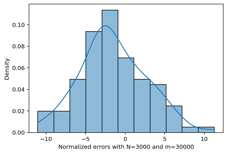
In this section, we assess the asymptotic normality of the approximate LSE θ^=(λN,m,νN,m)\hat{\theta}=(\lambda^{N,m},\nu^{N,m}) as established in Theorem 3.2. Specifically, we numerically verify that the normalized error term N((λN,mλ),(νN,mν))\sqrt{N}\big{(}(\lambda^{N,m}-\lambda),(\nu^{N,m}-\nu)\big{)} converges to a Gaussian distribution as NN and mm approach infinity.

We utilize the simulated 100 samples from the power of two choices model with the true parameter θ=(λ,ν)=(0.5,1)\theta=(\lambda,\nu)=(0.5,1), varying the network size NN and the number of observations mm. For each combination of (N,m)(N,m), we compute the first four empirical moments of the normalized error terms N((λN,mλ),(νN,mν))\sqrt{N}\big{(}(\lambda^{N,m}-\lambda),(\nu^{N,m}-\nu)\big{)}: the mean, variance, skewness, and kurtosis. The results are summarized in Table 2. Notably, we observe that the skewness and kurtosis values tend to approximate those of a normal distribution (0 for skewness and 3 for kurtosis), even for relatively small values of network size NN and number of observations mm.

Normalized error moments Mean Variance Skewness Kurtosis
N=100,m=1000 (5.37,6.60)(-5.37,-6.60) (1.75,2.07)(1.75,2.07) (0.16,0.41)(-0.16,-0.41) (3.44,4.31)(3.44,4.31)
N=500,m=10000 (7.15,8.65)(-7.15,-8.65) (8.99,11.32)(8.99,11.32) (0.51,0.60)(0.51,0.60) (3.90,4.21)(3.90,4.21)
N=1000,m=10000 (6.89,8.08)(-6.89,-8.08) (11.08,14.38)(11.08,14.38) (0.01,0.02)(0.01,0.02) (2.72,2.51)(2.72,2.51)
N=2000, m=20000 (1.47,2.01)(-1.47,-2.01) (13.96,15.59)(13.96,15.59) (0.07,0.20)(0.07,0.20) (2.80,2.68)(2.80,2.68)
N=3000, m=30000 (0.86,1.48)(-0.86,-1.48) (17.00,17.15)(17.00,17.15) (0.10,0.26)(0.10,0.26) (3.40,3.07)(3.40,3.07)
Table 2: Empirical moments of the normalized errors N((λN,mλ),(νN,mν))\sqrt{N}\big{(}(\lambda^{N,m}-\lambda),(\nu^{N,m}-\nu)\big{)}

To further substantiate our findings, we test the normality of the normalized error terms using a Kolmogorov-Smirnov test. We conduct this test on the 100100 simulated datasets across the different values of network size NN and number of observations mm. The resulting pp-values are presented in Table 3. As shown, the pp-values are sufficiently large, suggesting that the null hypothesis asserting that the error terms N((λN,mλ),(νN,mν))\sqrt{N}\big{(}(\lambda^{N,m}-\lambda),(\nu^{N,m}-\nu)\big{)} follow a normal distribution is not rejected, even for smaller values of NN and mm. This result indicates that the error terms tend to the normal distribution quickly. Nevertheless, it is also noted that the pp-values are high for all (N,m)(N,m) combinations, and they do not necessarily increase with larger network sizes NN and higher numbers of observations mm. This effect may be attributed to the fact that the true mean and variance of the error terms are unknown, requiring the use of empirical values, which may account for the observed outcomes.

Network and data sizes (N,m)(N,m) P-value for N(λN,mλ)\sqrt{N}(\lambda^{N,m}-\lambda) P-value for N(νN,mν)\sqrt{N}(\nu^{N,m}-\nu)
(N,m)=(100,1000)(N,m)=(100,1000) 0.710.71 0.480.48
(N,m)=(500,10000)(N,m)=(500,10000) 0.550.55 0.590.59
(N,m)=(1000,10000)(N,m)=(1000,10000) 0.990.99 0.330.33
(N,m)=(2000,20000)(N,m)=(2000,20000) 0.970.97 0.940.94
(N,m)=(3000,30000)(N,m)=(3000,30000) 0.650.65 0.660.66
Table 3: Kolmogorov-Smirnov tests for the normalized parameter estimator errors N((λN,mλ),(νN,mν))\sqrt{N}\big{(}(\lambda^{N,m}-\lambda),(\nu^{N,m}-\nu)\big{)}

Finally, we plot the histograms of the normalized error terms N((λN,mλ))\sqrt{N}\big{(}(\lambda^{N,m}-\lambda)\big{)} and N((νN,mν))\sqrt{N}\big{(}(\nu^{N,m}-\nu)\big{)}, along with a kernel density estimator. The results are shown in Figure 5 and Figure 6. Once again, we observe that the assertion of normality for the error terms aligns well with the empirical data.

Refer to caption
Refer to caption
Refer to caption
Refer to caption
Refer to caption
Figure 5: Histograms of the normalized errors N(λN,mλ)\sqrt{N}(\lambda^{N,m}-\lambda) with the associated kernel density estimate plots for different values of the network size NN and the number of observations mm with the true parameters θ=(λ,ν)=(0.5,1)\theta=(\lambda,\nu)=(0.5,1)
Refer to caption
Refer to caption
Refer to caption
Refer to caption
Refer to caption
Figure 6: Histograms of the normalized errors N(νN,mν)\sqrt{N}(\nu^{N,m}-\nu) with the associated kernel density estimate plots for different values of the network size NN and the number of observations mm, corresponding to true parameters θ=(λ,ν)=(0.5,1)\theta=(\lambda,\nu)=(0.5,1)

5 Conclusions and perspectives

In this paper, we considered the parameter estimation problem of the supermarket model. Based on an aggregate dataset, we constructed an approximate LSE by exploiting the law of large numbers together with the central limit theorem established for the model in the literature. Moreover, we proved the consistency together with the asymptotic normality of the estimator as both the size of the network and the number of observations go to infinity. Finally, we presented a numerical study where we tested our estimator against synthetic data obtained by simulating the power-of-two model highlighting our theoretical results.

The current work is the first statistical scheme for mean-field queuing systems and opens a new perspective. One naturally aims to investigate the statistical inference problem for other models. For instance, one can investigate the approximate LSE approach to the model proposed in [6] for load balancing mechanisms in cloud storage systems which is a generalization of the supermarket model. The established law of large numbers together with the central limit theorem make the approximate LSE approach used in the current work conceivable, provided that one can overcome the technical difficulty arising from the more complicated mean-field limiting equation. Another variation of the supermarket model for which one can study the parameter estimation problem is the one introduced in [7] in which the servers can communicate with their neighbors and where the neighborhood relationships are described in terms of a suitable graph. Again, the limit as the number of servers goes to infinity was identified, which can be exploited to build a statistical scheme, however, no central limit theorem nor a stationary distribution was established, therefore, the asymptotic normality of the estimator cannot be obtained by the similar scheme used in the current paper. Another interesting open problem is the nonparametric estimation of the interaction kernel in general mean-field queuing systems studied in [11]. Indeed, one can consider the exploitation of the limiting mean-field equation to build an estimator. However, contrary to our current proposal where the unknown parameters enter linearly in the mean-field limiting equation, in the nonparametric estimation one needs to deal with an optimization problem in function space. A potential avenue is to exploit the stationary distribution to build an estimator in the stationary regime and then investigate a justification for the interchange of limits NN\rightarrow\infty and tt\rightarrow\infty.

Finally, the problem of statistical inference for general mean-field models on discrete space remains open and, as mentioned in the introduction, very few references exist.

Appendix A Proof of Propositoin 2.1

Let ξ(t)=(ξj(t))T\xi(t)=(\xi_{j}(t))^{T} be the solution to the following infinite-dimensional ODE:

dξ(t)=G(M(t)+ξ(t),ϱ(t))dt,ξ(0)=z0~2.d\xi(t)=G\left(M(t)+\xi(t),\varrho(t)\right)dt,\quad\xi(0)=z_{0}\in\tilde{\ell}_{2}.

Define 𝒵(t):=M(t)+ξ(t){\cal Z}(t):=M(t)+\xi(t). Then, 𝒵(t){\cal Z}(t) satisfies the SDE:

d𝒵(t)=G(𝒵(t),ϱ(t))dt+a(t)dW(t),𝒵(0)=z0.d{\cal Z}(t)=G({\cal Z}(t),\varrho(t))dt+a(t)dW(t),\quad{\cal Z}(0)=z_{0}.

By [6, Proposition 2], we know that 𝒵(t)~2{\cal Z}(t)\in\tilde{\ell}_{2} for all t[0,T]t\in[0,T] almost surely. By the estimate [6, Page 69, line -1] and Fatou’s lemma (cf. [6, Page 78, Proof of Theorem 2]), we get

E[supt[0,T]m=0(m+1)2Mm2(t)]<.E\Bigg{[}\sup_{t\in[0,T]}\sum_{m=0}^{\infty}(m+1)^{2}M_{m}^{2}(t)\Bigg{]}<\infty.

Then, M(t),ξ(t)1M(t),\xi(t)\in\ell_{1} for all t[0,T]t\in[0,T] almost surely. Moreover, for any j+j\in\mathbb{Z}_{+}, we have ξj(0)=(z0)j\xi_{j}(0)=(z_{0})_{j}, and

dξj(t)dt\displaystyle\frac{d\xi_{j}(t)}{dt} =\displaystyle= Gj(𝒵(t),ϱ(t))\displaystyle G_{j}({\cal Z}(t),\varrho(t)) (A.1)
=\displaystyle= 2λm=j{[Mj1(t)+ξj1(t)]ϱm(t)+[Mm(t)+ξm(t)]ϱj1(t)\displaystyle 2\lambda\sum_{m=j}^{\infty}\{[M_{j-1}(t)+\xi_{j-1}(t)]\varrho_{m}(t)+[M_{m}(t)+\xi_{m}(t)]\varrho_{j-1}(t)
[Mj(t)+ξj(t)]ϱm+1(t)[Mm+1(t)+ξm+1(t)]ϱj(t)}\displaystyle\ \ \ \ \ \ \ \ \ \ -[M_{j}(t)+\xi_{j}(t)]\varrho_{m+1}(t)-[M_{m+1}(t)+\xi_{m+1}(t)]\varrho_{j}(t)\}
+ν{[Mj+1(t)+ξj+1(t)][Mj(t)+ξj(t)]}\displaystyle+\nu\{[M_{j+1}(t)+\xi_{j+1}(t)]-[M_{j}(t)+\xi_{j}(t)]\}
=\displaystyle= 2λ[Mj1(t)Mj(t)]m=jϱm(t)+2λ[ξj1(t)ξj(t)]m=jϱm(t)\displaystyle 2\lambda[M_{j-1}(t)-M_{j}(t)]\sum_{m=j}^{\infty}\varrho_{m}(t)+2\lambda[\xi_{j-1}(t)-\xi_{j}(t)]\sum_{m=j}^{\infty}\varrho_{m}(t)
+2λ[ϱj1(t)ϱj(t)]m=j[Mm(t)+ξm(t)]+2λMj(t)ϱj(t)+2λξj(t)ϱj(t)+2λϱj(t)[Mj(t)+ξj(t)]\displaystyle+2\lambda[\varrho_{j-1}(t)-\varrho_{j}(t)]\sum_{m=j}^{\infty}[M_{m}(t)+\xi_{m}(t)]+2\lambda M_{j}(t)\varrho_{j}(t)+2\lambda\xi_{j}(t)\varrho_{j}(t)+2\lambda\varrho_{j}(t)[M_{j}(t)+\xi_{j}(t)]
+ν{[Mj+1(t)Mj(t)]+[ξj+1(t)ξj(t)]}\displaystyle+\nu\{[M_{j+1}(t)-M_{j}(t)]+[\xi_{j+1}(t)-\xi_{j}(t)]\}
=\displaystyle= 2λ[Mj1(t)Mj(t)]m=jϱm(t)+2λ[ϱj1(t)ϱj(t)]m=jMm(t)+ν[Mj+1(t)Mj(t)]\displaystyle 2\lambda[M_{j-1}(t)-M_{j}(t)]\sum_{m=j}^{\infty}\varrho_{m}(t)+2\lambda[\varrho_{j-1}(t)-\varrho_{j}(t)]\sum_{m=j}^{\infty}M_{m}(t)+\nu[M_{j+1}(t)-M_{j}(t)]
+4λMj(t)ϱj(t)+4λξj(t)ϱj(t)\displaystyle+4\lambda M_{j}(t)\varrho_{j}(t)+4\lambda\xi_{j}(t)\varrho_{j}(t)
+2λ[ϱj1(t)ϱj(t)]m=jξm(t)+2λ[ξj1(t)ξj(t)]m=jϱm(t)+ν[ξj+1(t)ξj(t)]\displaystyle+2\lambda[\varrho_{j-1}(t)-\varrho_{j}(t)]\sum_{m=j}^{\infty}\xi_{m}(t)+2\lambda[\xi_{j-1}(t)-\xi_{j}(t)]\sum_{m=j}^{\infty}\varrho_{m}(t)+\nu[\xi_{j+1}(t)-\xi_{j}(t)]
=\displaystyle= 2λ(m=jϱm(t))[Mj1(t)Mj(t)]+2λ[ϱj1(t)ϱj(t)]m=jMm(t)+4λϱj(t)Mj(t)+ν[Mj+1(t)Mj(t)]\displaystyle 2\lambda\left(\sum_{m=j}^{\infty}\varrho_{m}(t)\right)[M_{j-1}(t)-M_{j}(t)]+2\lambda[\varrho_{j-1}(t)-\varrho_{j}(t)]\sum_{m=j}^{\infty}M_{m}(t)+4\lambda\varrho_{j}(t)M_{j}(t)+\nu[M_{j+1}(t)-M_{j}(t)]
+2λ[ϱj1(t)ϱj(t)]m=j+2ξm(t)+{2λ[ϱj1(t)ϱj(t)]+ν}ξj+1(t)\displaystyle+2\lambda[\varrho_{j-1}(t)-\varrho_{j}(t)]\sum_{m=j+2}^{\infty}\xi_{m}(t)+\{2\lambda[\varrho_{j-1}(t)-\varrho_{j}(t)]+\nu\}\xi_{j+1}(t)
+{2λ[ϱj1(t)+ϱj(t)m=jϱm(t)]ν}ξj(t)+2λ(m=jϱm(t))ξj1(t).\displaystyle+\left\{2\lambda\left[\varrho_{j-1}(t)+\varrho_{j}(t)-\sum_{m=j}^{\infty}\varrho_{m}(t)\right]-\nu\right\}\xi_{j}(t)+2\lambda\left(\sum_{m=j}^{\infty}\varrho_{m}(t)\right)\xi_{j-1}(t).

Since m=0𝒵m(t)=0\sum_{m=0}^{\infty}{\cal Z}_{m}(t)=0, we get

m=j+2ξm(t)=m=0Mm(t)m=0j+1ξm(t).\sum_{m=j+2}^{\infty}\xi_{m}(t)=-\sum_{m=0}^{\infty}M_{m}(t)-\sum_{m=0}^{j+1}\xi_{m}(t).

Similarly, by m=0ϱm(t)=1\sum_{m=0}^{\infty}\varrho_{m}(t)=1, we get

m=jϱm(t)=1m=0j1ϱm(t).\sum_{m=j}^{\infty}\varrho_{m}(t)=1-\sum_{m=0}^{j-1}\varrho_{m}(t).

Then, we can rewrite (A.1) as follows:

dξj(t)dt\displaystyle\frac{d\xi_{j}(t)}{dt} =\displaystyle= 2λ[1m=0j1ϱm(t)][Mj1(t)Mj(t)]2λ[ϱj1(t)ϱj(t)]m=0j1Mm(t)+4λϱj(t)Mj(t)+ν[Mj+1(t)Mj(t)]\displaystyle 2\lambda\left[1-\sum_{m=0}^{j-1}\varrho_{m}(t)\right][M_{j-1}(t)-M_{j}(t)]-2\lambda[\varrho_{j-1}(t)-\varrho_{j}(t)]\sum_{m=0}^{j-1}M_{m}(t)+4\lambda\varrho_{j}(t)M_{j}(t)+\nu[M_{j+1}(t)-M_{j}(t)] (A.2)
2λ[ϱj1(t)ϱj(t)]m=0j2ξm(t)+2λ[1m=0j2ϱm(t)2ϱj1(t)+ϱj(t)]ξj1(t)\displaystyle-2\lambda[\varrho_{j-1}(t)-\varrho_{j}(t)]\sum_{m=0}^{j-2}\xi_{m}(t)+2\lambda\left[1-\sum_{m=0}^{j-2}\varrho_{m}(t)-2\varrho_{j-1}(t)+\varrho_{j}(t)\right]\xi_{j-1}(t)
+{2λ[1+m=0j1ϱm(t)+2ϱj(t)]ν}ξj(t)+νξj+1(t).\displaystyle+\left\{2\lambda\left[-1+\sum_{m=0}^{j-1}\varrho_{m}(t)+2\varrho_{j}(t)\right]-\nu\right\}\xi_{j}(t)+\nu\xi_{j+1}(t).

Note that (A.2) can be regarded as an infinite-dimensional non-autonomous linear system of ODEs with random coefficients. Define g(t)=(gj(t))j=0g(t)=(g_{j}(t))_{j=0}^{\infty} and C(t)=(Cjl(t))j,l=0C(t)=(C_{jl}(t))_{j,l=0}^{\infty} by

gj(t)\displaystyle g_{j}(t) :=\displaystyle:= 2λ[1m=0j1ϱm(t)][Mj1(t)Mj(t)]2λ[ϱj1(t)ϱj(t)]m=0j1Mm(t)\displaystyle 2\lambda\left[1-\sum_{m=0}^{j-1}\varrho_{m}(t)\right][M_{j-1}(t)-M_{j}(t)]-2\lambda[\varrho_{j-1}(t)-\varrho_{j}(t)]\sum_{m=0}^{j-1}M_{m}(t) (A.3)
+4λϱj(t)Mj(t)+ν[Mj+1(t)Mj(t)]\displaystyle+4\lambda\varrho_{j}(t)M_{j}(t)+\nu[M_{j+1}(t)-M_{j}(t)]
=\displaystyle= 2λ[ϱj1(t)ϱj(t)]m=0j2Mm(t)+2λ[1m=0j2ϱm(t)2ϱj1(t)+ϱj(t)]Mj1(t)\displaystyle-2\lambda[\varrho_{j-1}(t)-\varrho_{j}(t)]\sum_{m=0}^{j-2}M_{m}(t)+2\lambda\left[1-\sum_{m=0}^{j-2}\varrho_{m}(t)-2\varrho_{j-1}(t)+\varrho_{j}(t)\right]M_{j-1}(t)
+{2λ[1+m=0j1ϱm(t)+2ϱj(t)]ν}Mj(t)+νMj+1(t),\displaystyle+\left\{2\lambda\left[-1+\sum_{m=0}^{j-1}\varrho_{m}(t)+2\varrho_{j}(t)\right]-\nu\right\}M_{j}(t)+\nu M_{j+1}(t),

and

Cjl(t):={2λ[ϱj1(t)ϱj(t)],if 0lj2,2λ[1m=0j2ϱm(t)2ϱj1(t)+ϱj(t)],if l=j1,2λ[1+m=0j1ϱm(t)+2ϱj(t)]ν,if l=j,ν,if l=j+1,0,if lj+2.\displaystyle C_{jl}(t):=\left\{\begin{array}[]{ll}-2\lambda[\varrho_{j-1}(t)-\varrho_{j}(t)],&\mbox{if $0\leq l\leq j-2$},\\ 2\lambda\left[1-\sum_{m=0}^{j-2}\varrho_{m}(t)-2\varrho_{j-1}(t)+\varrho_{j}(t)\right],&\mbox{if $l=j-1$},\\ 2\lambda\left[-1+\sum_{m=0}^{j-1}\varrho_{m}(t)+2\varrho_{j}(t)\right]-\nu,&\mbox{if $l=j$},\\ \nu,&\mbox{if $l=j+1$},\\ 0,&\mbox{if $l\geq j+2$}.\end{array}\right. (A.9)

Then, (A.2) becomes

dξ(t)dt=C(t)ξ(t)+g(t),ξ(0)=z0.\frac{d\xi(t)}{dt}=C(t)\xi(t)+g(t),\quad\xi(0)=z_{0}.

Denote 𝒞=6λ+ν.{\cal C}=6\lambda+\nu. Therefore, for any j+j\in\mathbb{Z}_{+} and t[0,T]t\in[0,T], by (A.3), we get

|gj(t)|𝒞{|Mj1(t)|+|Mj(t)|+|Mj+1(t)|+[ϱj1(t)+ϱj(t)][π26supt[0,T]m=0(m+1)2Mm2(t)]12}.\displaystyle|g_{j}(t)|\leq{\cal C}\Bigg{\{}|M_{j-1}(t)|+|M_{j}(t)|+|M_{j+1}(t)|+[\varrho_{j-1}(t)+\varrho_{j}(t)]\Bigg{[}\frac{\pi^{2}}{6}\sup_{t\in[0,T]}\sum_{m=0}^{\infty}(m+1)^{2}M^{2}_{m}(t)\Bigg{]}^{\frac{1}{2}}\Bigg{\}}.

Then,

supt[0,T]g(t)15𝒞[π26supt[0,T]m=0(m+1)2Mm2(t)]12.\displaystyle\sup_{t\in[0,T]}\|g(t)\|_{1}\leq 5{\cal C}\Bigg{[}\frac{\pi^{2}}{6}\sup_{t\in[0,T]}\sum_{m=0}^{\infty}(m+1)^{2}M^{2}_{m}(t)\Bigg{]}^{\frac{1}{2}}.

For x1x\in\ell_{1}, j+j\in\mathbb{Z}_{+} and t[0,T]t\in[0,T], by (A.9), we get

|(C(t)x)j|𝒞{[ϱj1(t)+ϱj(t)]l=0j2|xl|+|xj1|+|xj|+|xj+1|}.\displaystyle|(C(t)x)_{j}|\leq{\cal C}\Bigg{\{}[\varrho_{j-1}(t)+\varrho_{j}(t)]\sum_{l=0}^{j-2}|x_{l}|+|x_{j-1}|+|x_{j}|+|x_{j+1}|\Bigg{\}}.

Then,

C(t)x15𝒞x1.\displaystyle\|C(t)x\|_{1}\leq 5{\cal C}\|x\|_{1}.

Hence, by induction, we obtain that

[C(t)]nx1(5𝒞)nx1,n.\|[C(t)]^{n}x\|_{1}\leq(5{\cal C})^{n}\|x\|_{1},\quad n\in\mathbb{N}.

Thus, we have the following explicit expressions:

ξ(t)=e0tC(s)𝑑sz0+0testC(u)𝑑ug(s)𝑑s,𝒵(t)=M(t)+ξ(t).\displaystyle\xi(t)=e^{\int_{0}^{t}C(s)ds}z_{0}+\int_{0}^{t}e^{\int_{s}^{t}C(u)du}g(s)ds,\ \ \ \ {\cal Z}(t)=M(t)+\xi(t). (A.10)

Since M(t)M(t) is a Gaussian martingale, by (A.3), we deduce that the distributions of ξ(t)\xi(t) and 𝒵(t){\cal Z}(t) are both Gaussian. The proof is complete.

Appendix B Proof of Lemma 3.1

By Hölder’s inequality, we find that a11a22(a12)2a_{11}a_{22}\geq(a_{12})^{2} and the equality sign holds if and only if a11=0a_{11}=0, or a22=0a_{22}=0, or

a11,a22>0anda_{11},a_{22}>0\ \ \ \ {\rm and}\ \ \ \

for all j+j^{\prime}\in\mathbb{Z}_{+} (see, e.g. [33])

0TUj(ϱ(s,θ))𝑑s(j=0[0TUj(ϱ(s,θ))𝑑s]2)12=0TVj(ϱ(s,θ))𝑑s(j=0[0TVj(ϱ(s,θ))𝑑s]2)12.\begin{split}&\frac{\int_{0}^{T}U_{j^{\prime}}(\varrho(s,\theta^{*}))ds}{\bigg{(}\sum\limits_{j=0}^{\infty}\left[\int_{0}^{T}U_{j}(\varrho(s,\theta^{*}))ds\right]^{2}\bigg{)}^{\frac{1}{2}}}=\frac{\int_{0}^{T}V_{j^{\prime}}(\varrho(s,\theta^{*}))ds}{\bigg{(}\sum\limits_{j=0}^{\infty}\left[\int_{0}^{T}V_{j}(\varrho(s,\theta^{*}))ds\right]^{2}\bigg{)}^{\frac{1}{2}}}.\end{split} (B.1)

Note that for s[0,T]s\in[0,T],

U0(ϱ(s,θ))=2ϱ0(s,θ)i=1ϱi(s,θ)(ϱ0(s,θ))2,\displaystyle\begin{split}U_{0}(\varrho(s,\theta^{*}))=-2\varrho_{0}(s,\theta^{*})\sum_{i=1}^{\infty}\varrho_{i}(s,\theta^{*})-(\varrho_{0}(s,\theta^{*}))^{2},\end{split}

and

U1(ϱ(s,θ))=2ϱ0(s,θ)i=1ϱi(s,θ)2ϱ1(s,θ)i=2ϱi(s,θ)+(ϱ0(s,θ))2(ϱ1(s,θ))2,\displaystyle\begin{split}U_{1}(\varrho(s,\theta^{*}))=2\varrho_{0}(s,\theta^{*})\sum_{i=1}^{\infty}\varrho_{i}(s,\theta^{*})-2\varrho_{1}(s,\theta^{*})\sum_{i=2}^{\infty}\varrho_{i}(s,\theta^{*})+(\varrho_{0}(s,\theta^{*}))^{2}-(\varrho_{1}(s,\theta^{*}))^{2},\end{split}

Then, by the fact that i=0ϱi(s,θ)=1\sum\limits_{i=0}^{\infty}\varrho_{i}(s,\theta^{*})=1, we get

U0(ϱ(s,θ))=2ϱ0(s,θ)(1ϱ0(s,θ))(ϱ0(s,θ))2=ϱ0(s,θ)(ϱ0(s,θ)2),\displaystyle\begin{split}U_{0}(\varrho(s,\theta^{*}))&=-2\varrho_{0}(s,\theta^{*})(1-\varrho_{0}(s,\theta^{*}))-(\varrho_{0}(s,\theta^{*}))^{2}=\varrho_{0}(s,\theta^{*})(\varrho_{0}(s,\theta^{*})-2),\end{split}

and

U1(ϱ(s,θ))=2ϱ0(s,θ)(1ϱ0(s,θ))2ϱ1(s,θ)(1ϱ0(s,θ)ϱ1(s,θ))+(ϱ0(s,θ))2(ϱ1(s,θ))2=(ϱ0(s,θ)ϱ1(s,θ))(2ϱ0(s,θ))+(ϱ1(s,θ))(ϱ0(s,θ)+ϱ1(s,θ)).\displaystyle\begin{split}U_{1}(\varrho(s,\theta^{*}))&=2\varrho_{0}(s,\theta^{*})(1-\varrho_{0}(s,\theta^{*}))-2\varrho_{1}(s,\theta^{*})(1-\varrho_{0}(s,\theta^{*})-\varrho_{1}(s,\theta^{*}))+(\varrho_{0}(s,\theta^{*}))^{2}-(\varrho_{1}(s,\theta^{*}))^{2}\\ &=(\varrho_{0}(s,\theta^{*})-\varrho_{1}(s,\theta^{*}))(2-\varrho_{0}(s,\theta^{*}))+(\varrho_{1}(s,\theta^{*}))(\varrho_{0}(s,\theta^{*})+\varrho_{1}(s,\theta^{*})).\end{split}

We have

V0(ϱ(s,θ))=ϱ1(s,θ)ϱ0(s,θ),V_{0}(\varrho(s,\theta^{*}))=\varrho_{1}(s,\theta^{*})-\varrho_{0}(s,\theta^{*}),

and

V1(ϱ(s,θ))=ϱ2(s,θ)ϱ1(s,θ).V_{1}(\varrho(s,\theta^{*}))=\varrho_{2}(s,\theta^{*})-\varrho_{1}(s,\theta^{*}).

(a) Suppose that (3.8)(\ref{cond-ineq-posed1}) holds. Then, 0TU0(ϱ(s,θ))𝑑s<0\int_{0}^{T}U_{0}(\varrho(s,\theta^{*}))ds<0 and 0TV0(ϱ(s,θ))𝑑s>0\int_{0}^{T}V_{0}(\varrho(s,\theta^{*}))ds>0. Thus, (B.1)(\ref{Hold-ineq}) cannot hold and hence (3.7)(\ref{equal-Hold}) holds. (b) Suppose that (3.9)(\ref{cond-ineq-posed2}) holds. Then, 0TU1(ϱ(s,θ))𝑑s>0\int_{0}^{T}U_{1}(\varrho(s,\theta^{*}))ds>0 and 0TV1(ϱ(s,θ))𝑑s<0\int_{0}^{T}V_{1}(\varrho(s,\theta^{*}))ds<0. Thus, (B.1)(\ref{Hold-ineq}) cannot hold and hence (3.7)(\ref{equal-Hold}) holds.

Appendix C Proof of Theorem 3.1

By Theorem 2.1, [15, (5.7), page 117 and Proposition 5.3, page 119] and Lemma 3.2, we obtain that

supt[0,T]j=0|ϱjN(t,θ)ϱj(t,θ)|0\sup_{t\in[0,T]}\sum_{j=0}^{\infty}|\varrho^{N}_{j}(t,\theta^{*})-\varrho_{j}(t,\theta^{*})|\rightarrow 0 (C.1)

in probability as NN\rightarrow\infty. Moreover,

|a11N,ma11|j=0|[Tmk=1mUj(ϱN(tk,θ))]2[0TUj(ϱ(s))𝑑s]2|supj+{|Tmk=1mUj(ϱN(tk,θ))+0TUj(ϱ(s))𝑑s|}×j=0|Tmk=1mUj(ϱN(tk,θ))0TUj(ϱ(s))ds|Tsupj+{supt[0,T]|Uj(ϱN(t,θ))|+supt[0,T]|Uj(ϱ(t,θ))|}×j=0{|Tmk=1mUj(ϱN(tk,θ))Tmk=1mUj(ϱ(tk,θ))|+|Tmk=1mUj(ϱ(tk,θ))0TUj(ϱ(s))ds|}.\begin{split}|a^{N,m}_{11}-a_{11}|&\leq\sum\limits_{j=0}^{\infty}\left|\left[\frac{T}{m}\sum\limits_{k=1}^{m}U_{j}(\varrho^{N}(t_{k},\theta^{*}))\right]^{2}-\left[\int_{0}^{T}U_{j}(\varrho(s))ds\right]^{2}\right|\\ &\leq{\sup_{j\in\mathbb{Z}_{+}}}\bigg{\{}\left|\frac{T}{m}\sum\limits_{k=1}^{m}U_{j}(\varrho^{N}(t_{k},\theta^{*}))+\int_{0}^{T}U_{j}(\varrho(s))ds\right|\bigg{\}}\\ &\qquad\times\sum\limits_{j=0}^{\infty}\left|\frac{T}{m}\sum\limits_{k=1}^{m}U_{j}(\varrho^{N}(t_{k},\theta^{*}))-\int_{0}^{T}U_{j}(\varrho(s))ds\right|\\ &\leq T{\sup_{j\in\mathbb{Z}_{+}}\Big{\{}\sup_{t\in[0,T]}\big{|}U_{j}(\varrho^{N}(t,\theta^{*}))\big{|}+\sup_{t\in[0,T]}\big{|}U_{j}(\varrho(t,\theta^{*}))\big{|}\Big{\}}}\\ &\qquad\times\sum\limits_{j=0}^{\infty}\bigg{\{}\left|\frac{T}{m}\sum\limits_{k=1}^{m}U_{j}(\varrho^{N}(t_{k},\theta^{*}))-\frac{T}{m}\sum\limits_{k=1}^{m}U_{j}(\varrho(t_{k},\theta^{*}))\right|\\ &\qquad\quad\qquad+\left|\frac{T}{m}\sum\limits_{k=1}^{m}U_{j}(\varrho(t_{k},\theta^{*}))-\int_{0}^{T}U_{j}(\varrho(s))ds\right|\bigg{\}}.\end{split}

By (3.1), we get |Uj(x)|6x1|U_{j}(x)|\leq 6\|x\|_{1} for all x1x\in\ell_{1} and j+j\in\mathbb{Z}_{+}. Then

|a11N,ma11|\displaystyle|a^{N,m}_{11}-a_{11}| 12T{Tsupt[0,T]j=0|Uj(ϱN(t,θ))Uj(ϱ(t,θ))|\displaystyle\leq 12T\bigg{\{}T\sup_{t\in[0,T]}\sum\limits_{j=0}^{\infty}\left|U_{j}(\varrho^{N}(t,\theta^{*}))-U_{j}(\varrho(t,\theta^{*}))\right|
+j=0|Tmk=1mUj(ϱ(tk,θ))0TUj(ϱ(s))ds|}.\displaystyle\qquad\quad+\sum\limits_{j=0}^{\infty}\left|\frac{T}{m}\sum\limits_{k=1}^{m}U_{j}(\varrho(t_{k},\theta^{*}))-\int_{0}^{T}U_{j}(\varrho(s))ds\right|\bigg{\}}.

Therefore, by (C.1), we get that the right hand side of the last inequality goes to 0inprobabilityasN,m0\ \ {\rm in\ probability}\ {\rm as}\ N,m\rightarrow\infty. Similarly, we can show that

|a12N,ma12|,|a22N,ma22|,|b1N,mb1|,|b2N,mb2|0inprobabilityasN,m.|a^{N,m}_{12}-a_{12}|,\,|a^{N,m}_{22}-a_{22}|,\,|b^{N,m}_{1}-b_{1}|,\,|b^{N,m}_{2}-b_{2}|\rightarrow 0\ \ {\rm in\ probability}\ {\rm as}\ N,m\rightarrow\infty.

Therefore, the proof is complete.

Appendix D Proof of Theorem 3.2

By (3.6)(\ref{lambda-nu-star}) and (3.10)(\ref{Nov1b}), we get

N((λN,mνN,m)(λν))=N(a22N,mb1N,ma12N,mb2N,ma11N,ma22N,m(a12N,m)2a22b1a12b2a11a22(a12)2a21N,mb1N,m+a11N,mb2N,ma11N,ma22N,m(a12N,m)2a21b1+a11b2a11a22(a12)2).\begin{split}\sqrt{N}\bigg{(}\begin{pmatrix}\lambda^{N,m}\\ \nu^{N,m}\end{pmatrix}-\begin{pmatrix}\lambda^{*}\\ \nu^{*}\end{pmatrix}\bigg{)}=\sqrt{N}\begin{pmatrix}\frac{a^{N,m}_{22}b^{N,m}_{1}-a^{N,m}_{12}b^{N,m}_{2}}{a^{N,m}_{11}a^{N,m}_{22}-(a^{N,m}_{12})^{2}}-\frac{a_{22}b_{1}-a_{12}b_{2}}{a_{11}a_{22}-(a_{12})^{2}}\\ \\ \frac{-a^{N,m}_{21}b^{N,m}_{1}+a^{N,m}_{11}b^{N,m}_{2}}{a^{N,m}_{11}a^{N,m}_{22}-(a^{N,m}_{12})^{2}}-\frac{-a_{21}b_{1}+a_{11}b_{2}}{a_{11}a_{22}-(a_{12})^{2}}\end{pmatrix}.\end{split}

Moreover, simple calculations lead to

a22N,mb1N,ma12N,mb2N,ma11N,ma22N,m(a12N,m)2a22b1a12b2a11a22(a12)2=(a22N,mb1N,ma12N,mb2N,m)(a22b1a12b2)a11N,ma22N,m(a12N,m)2+(a22b1a12b2)[(a11a22(a12)2)(a11N,ma22N,m(a12N,m)2)](a11N,ma22N,m(a12N,m)2)(a11a22(a12)2),\begin{split}\frac{a^{N,m}_{22}b^{N,m}_{1}-a^{N,m}_{12}b^{N,m}_{2}}{a^{N,m}_{11}a^{N,m}_{22}-(a^{N,m}_{12})^{2}}-\frac{a_{22}b_{1}-a_{12}b_{2}}{a_{11}a_{22}-(a_{12})^{2}}&=\frac{(a^{N,m}_{22}b^{N,m}_{1}-a^{N,m}_{12}b^{N,m}_{2})-(a_{22}b_{1}-a_{12}b_{2})}{a^{N,m}_{11}a^{N,m}_{22}-(a^{N,m}_{12})^{2}}\\ &\quad+\frac{{(a_{22}b_{1}-a_{12}b_{2})[(a_{11}a_{22}-(a_{12})^{2})-(a^{N,m}_{11}a^{N,m}_{22}-(a^{N,m}_{12})^{2})]}}{(a^{N,m}_{11}a^{N,m}_{22}-(a^{N,m}_{12})^{2})(a_{11}a_{22}-(a_{12})^{2})},\end{split}

and

a21N,mb1N,m+a11N,mb2N,ma11N,ma22N,m(a12N,m)2a21b1+a11b2a11a22(a12)2=(a21N,mb1N,m+a11N,mb2N,m)(a21b1+a11b2)a11N,ma22N,m(a12N,m)2+(a21b1+a11b2)[(a11a22(a12)2)(a11N,ma22N,m(a12N,m)2)](a11N,ma22N,m(a12N,m)2)(a11a22(a12)2).\begin{split}\frac{-a^{N,m}_{21}b^{N,m}_{1}+a^{N,m}_{11}b^{N,m}_{2}}{a^{N,m}_{11}a^{N,m}_{22}-(a^{N,m}_{12})^{2}}-\frac{-a_{21}b_{1}+a_{11}b_{2}}{a_{11}a_{22}-(a_{12})^{2}}&=\frac{(-a^{N,m}_{21}b^{N,m}_{1}+a^{N,m}_{11}b^{N,m}_{2})-(-a_{21}b_{1}+a_{11}b_{2})}{a^{N,m}_{11}a^{N,m}_{22}-(a^{N,m}_{12})^{2}}\\ &\quad+\frac{{(-a_{21}b_{1}+a_{11}b_{2})[(a_{11}a_{22}-(a_{12})^{2})-(a^{N,m}_{11}a^{N,m}_{22}-(a^{N,m}_{12})^{2})]}}{(a^{N,m}_{11}a^{N,m}_{22}-(a^{N,m}_{12})^{2})(a_{11}a_{22}-(a_{12})^{2})}.\end{split}

To simplify notation, let us define

N,m:=N[(a22N,mb1N,ma12N,mb2N,m)(a22b1a12b2)],\displaystyle\mathcal{I}^{N,m}:=\sqrt{N}\bigg{[}(a^{N,m}_{22}b^{N,m}_{1}-a^{N,m}_{12}b^{N,m}_{2})-(a_{22}b_{1}-a_{12}b_{2})\bigg{]},
𝒥N,m:=N[(a21N,mb1N,m+a11N,mb2N,m)(a21b1+a11b2)],\displaystyle\mathcal{J}^{N,m}:=\sqrt{N}\bigg{[}(-a^{N,m}_{21}b^{N,m}_{1}+a^{N,m}_{11}b^{N,m}_{2})-(-a_{21}b_{1}+a_{11}b_{2})\bigg{]},
N,m:=a11N,ma22N,m(a12N,m)2,\displaystyle\mathcal{H}^{N,m}:=a^{N,m}_{11}a^{N,m}_{22}-(a^{N,m}_{12})^{2},

and

𝒦N,m:=N[(a11a22(a12)2)(a11N,ma22N,m(a12N,m)2)].\displaystyle\mathcal{K}^{N,m}:=\sqrt{N}\bigg{[}(a_{11}a_{22}-(a_{12})^{2})-(a^{N,m}_{11}a^{N,m}_{22}-(a^{N,m}_{12})^{2})\bigg{]}.

We will analyze the convergence of N,m,𝒥N,m\mathcal{I}^{N,m},\mathcal{J}^{N,m} and 𝒦N,m\mathcal{K}^{N,m} as N,m,mNN,m,\frac{m}{\sqrt{N}}\rightarrow\infty. By the Skorohod representation theorem (cf. [15, Page 102]), we can and do assume without loss of generality that 𝒵N\mathcal{Z}^{N} converges to 𝒵\mathcal{Z} in probability in 𝒟([0,T],2)\mathcal{D}([0,T],\ell_{2}). To save space, we will prove the convergence of N,m\mathcal{I}^{N,m}, the convergence of the other terms follows by similar arguments. First, we have

N,m=1N,m+2N,m\displaystyle\mathcal{I}^{N,m}=\mathcal{I}^{N,m}_{1}+\mathcal{I}^{N,m}_{2}

with

1N,m=N(a22N,mb1N,ma22b1) and 2N,m=N(a12b2a12N,mb2N,m).\displaystyle\mathcal{I}^{N,m}_{1}=\sqrt{N}\big{(}a^{N,m}_{22}b^{N,m}_{1}-a_{22}b_{1}\big{)}\ \ \mbox{ and }\ \ \mathcal{I}^{N,m}_{2}=\sqrt{N}\big{(}a_{12}b_{2}-a^{N,m}_{12}b^{N,m}_{2}\big{)}.

Moreover,

1N,m=Na22(b1N,mb1)+Nb1N,m(a22N,ma22),\displaystyle\mathcal{I}^{N,m}_{1}=\sqrt{N}a_{22}(b_{1}^{N,m}-b_{1})+\sqrt{N}b_{1}^{N,m}(a^{N,m}_{22}-a_{22}),

and

2N,m=N(a12(b2N,mb2)+b2N,m(a12N,ma12)).\displaystyle\mathcal{I}^{N,m}_{2}=-\sqrt{N}\big{(}a_{12}(b_{2}^{N,m}-b_{2})+b_{2}^{N,m}(a_{12}^{N,m}-a_{12})\big{)}.

Then, by adding and subtracting terms, we get

b1N,mb1\displaystyle b_{1}^{N,m}-b_{1}
=j=0[ϱj(T,θ)ϱj(0,θ)]{[Tmk=1mUj(ϱN(tk,θ))][Tmk=1mUj(ϱ(tk,θ))]}\displaystyle=\sum\limits_{j=0}^{\infty}\left[{\varrho}_{j}(T,\theta^{*})-{\varrho}_{j}(0,\theta^{*})\right]\Bigg{\{}\left[\frac{T}{m}\sum\limits_{k=1}^{m}U_{j}(\varrho^{N}(t_{k},\theta^{*}))\right]-\left[\frac{T}{m}\sum\limits_{k=1}^{m}U_{j}(\varrho(t_{k},\theta^{*}))\right]\Bigg{\}}
+j=0{[ϱjN(T,θ)ϱjN(0,θ)][ϱj(T,θ)ϱj(0,θ)]}{[Tmk=1mUj(ϱN(tk,θ))][Tmk=1mUj(ϱ(tk,θ))]}\displaystyle\quad+\sum\limits_{j=0}^{\infty}\Bigg{\{}\left[{\varrho}^{N}_{j}(T,\theta^{*})-{\varrho}^{N}_{j}(0,\theta^{*})\right]-\left[{\varrho}_{j}(T,\theta^{*})-{\varrho}_{j}(0,\theta^{*})\right]\Bigg{\}}\Bigg{\{}\left[\frac{T}{m}\sum\limits_{k=1}^{m}U_{j}(\varrho^{N}(t_{k},\theta^{*}))\right]-\left[\frac{T}{m}\sum\limits_{k=1}^{m}U_{j}(\varrho(t_{k},\theta^{*}))\right]\Bigg{\}}
+j=0[ϱjN(T,θ)ϱjN(0,θ)]{[Tmk=1mUj(ϱ(tk,θ))]0TUj(ϱ(s))𝑑s}\displaystyle\quad+\sum\limits_{j=0}^{\infty}\left[{\varrho}^{N}_{j}(T,\theta^{*})-{\varrho}^{N}_{j}(0,\theta^{*})\right]\Bigg{\{}\left[\frac{T}{m}\sum\limits_{k=1}^{m}U_{j}(\varrho(t_{k},\theta^{*}))\right]-\int_{0}^{T}U_{j}(\varrho(s))ds\Bigg{\}}
+j=0{[ϱjN(T,θ)ϱjN(0,θ)][ϱj(T,θ)ϱj(0,θ)]}0TUj(ϱ(s))𝑑s.\displaystyle\quad+\sum\limits_{j=0}^{\infty}\Bigg{\{}\left[{\varrho}^{N}_{j}(T,\theta^{*})-{\varrho}^{N}_{j}(0,\theta^{*})\right]-\left[{\varrho}_{j}(T,\theta^{*})-{\varrho}_{j}(0,\theta^{*})\right]\Bigg{\}}\int_{0}^{T}U_{j}(\varrho(s))ds. (D.1)

Below we consider the convergence of each summation term in (D). (a) By Theorem 2.2, as NN\rightarrow\infty, the term

Nj=0{[ϱjN(T,θ)ϱjN(0,θ)][ϱj(T,θ)ϱj(0,θ)]}0TUj(ϱ(s))𝑑s\displaystyle\sqrt{N}\sum\limits_{j=0}^{\infty}\Bigg{\{}\left[{\varrho}^{N}_{j}(T,\theta^{*})-{\varrho}^{N}_{j}(0,\theta^{*})\right]-\left[{\varrho}_{j}(T,\theta^{*})-{\varrho}_{j}(0,\theta^{*})\right]\Bigg{\}}\int_{0}^{T}U_{j}(\varrho(s))ds

converges in probability to

j=0[𝒵j(T,θ)𝒵j(0,θ)]0TUj(ϱ(s))𝑑s.\displaystyle\sum\limits_{j=0}^{\infty}\left[\mathcal{Z}_{j}(T,\theta^{*})-\mathcal{Z}_{j}(0,\theta^{*})\right]\int_{0}^{T}U_{j}(\varrho(s))ds.

(b) By (2.1) and (3.1)–(3.3), we get

|Uj(ϱ(tk,θ))Uj(ϱ(s))|\displaystyle|U_{j}(\varrho(t_{k},\theta^{*}))-U_{j}(\varrho(s))| \displaystyle\leq 2ϱj1(tk,θ)i=0|ϱi(tk,θ)ϱi(s,θ)|+2|ϱj1(tk,θ)ϱj1(s,θ)|\displaystyle 2\varrho_{j-1}(t_{k},\theta^{*})\sum_{i=0}^{\infty}\big{|}\varrho_{i}(t_{k},\theta^{*})-\varrho_{i}(s,\theta^{*})\big{|}+2\big{|}\varrho_{j-1}(t_{k},\theta^{*})-\varrho_{j-1}(s,\theta^{*})\big{|}
+2ϱj(tk,θ)i=0|ϱi(tk,θ)ϱi(s,θ)|+2|ϱj(tk,θ)ϱj(s,θ)|\displaystyle+2\varrho_{j}(t_{k},\theta^{*})\sum_{i=0}^{\infty}\big{|}\varrho_{i}(t_{k},\theta^{*})-\varrho_{i}(s,\theta^{*})\big{|}+2\big{|}\varrho_{j}(t_{k},\theta^{*})-\varrho_{j}(s,\theta^{*})\big{|}
+2|ϱj1(tk,θ)ϱj1(s,θ)|+2|ϱj(tk,θ)ϱj(s,θ)|\displaystyle+2\big{|}\varrho_{j-1}(t_{k},\theta^{*})-\varrho_{j-1}(s,\theta^{*})\big{|}+2\big{|}\varrho_{j}(t_{k},\theta^{*})-\varrho_{j}(s,\theta^{*})\big{|}
\displaystyle\leq 6i=0|ϱi(tk,θ)ϱi(s,θ)|\displaystyle 6\sum_{i=0}^{\infty}\big{|}\varrho_{i}(t_{k},\theta^{*})-\varrho_{i}(s,\theta^{*})\big{|}
\displaystyle\leq 6i=0stk|Fi(ϱ(u,θ))|𝑑u\displaystyle 6\sum_{i=0}^{\infty}\int_{s}^{t_{k}}\big{|}F_{i}(\varrho(u,\theta^{*}))\big{|}du
\displaystyle\leq 6(6λ+2ν)Tm.\displaystyle\frac{6(6\lambda+2\nu)T}{m}.

Then,

|Nj=0[ϱjN(T,θ)ϱjN(0,θ)]{[Tmk=1mUj(ϱ(tk,θ))]0TUj(ϱ(s))𝑑s}|=|Nj=0[ϱjN(T,θ)ϱjN(0,θ)]{k=1mtk1tk[Uj(ϱ(tk,θ))Uj(ϱ(s))]𝑑s}|Nj=0[ϱjN(T,θ)+ϱjN(0,θ)]{k=1mtk1tk6(6λ+2ν)Tm𝑑s}=24(3λ+ν)T2Nm0asmN.\begin{split}&\left|\sqrt{N}\sum\limits_{j=0}^{\infty}\left[{\varrho}^{N}_{j}(T,\theta^{*})-{\varrho}^{N}_{j}(0,\theta^{*})\right]\Bigg{\{}\left[\frac{T}{m}\sum\limits_{k=1}^{m}U_{j}(\varrho(t_{k},\theta^{*}))\right]-\int_{0}^{T}U_{j}(\varrho(s))ds\Bigg{\}}\right|\\ &\qquad=\left|\sqrt{N}\sum\limits_{j=0}^{\infty}\left[{\varrho}^{N}_{j}(T,\theta^{*})-{\varrho}^{N}_{j}(0,\theta^{*})\right]\Bigg{\{}\sum\limits_{k=1}^{m}\int_{t_{k-1}}^{t_{k}}[U_{j}(\varrho(t_{k},\theta^{*}))-U_{j}(\varrho(s))]ds\Bigg{\}}\right|\\ &\qquad\leq\sqrt{N}\sum\limits_{j=0}^{\infty}\left[{\varrho}^{N}_{j}(T,\theta^{*})+{\varrho}^{N}_{j}(0,\theta^{*})\right]\Bigg{\{}\sum\limits_{k=1}^{m}\int_{t_{k-1}}^{t_{k}}\frac{6(6\lambda+2\nu)T}{m}ds\Bigg{\}}\\ &\qquad=\frac{24(3\lambda+\nu)T^{2}\sqrt{N}}{m}\\ &\qquad\rightarrow 0\ \ \ \ {\rm as}\ \frac{m}{\sqrt{N}}\rightarrow\infty.\end{split}

(c) By the estimate [6, Page 70, line 4], we have that

supNE[supt[0,T]j=0(j+1)2(𝒵jN(t,θ))2]<.\sup_{N\in\mathbb{N}}E\left[\sup_{t\in[0,T]}\sum_{j=0}^{\infty}(j+1)^{2}({\cal Z}^{N}_{j}(t,\theta^{*}))^{2}\right]<\infty. (D.2)

Then, by Fatou’s lemma, we get

E[supt[0,T]j=0(j+1)2(𝒵j(t,θ))2]<.E\left[\sup_{t\in[0,T]}\sum_{j=0}^{\infty}(j+1)^{2}({\cal Z}_{j}(t,\theta^{*}))^{2}\right]<\infty. (D.3)

By (2.1) and (3.1)–(3.3), we get

|Uj(ϱN(tk,θ))Uj(ϱ(tk,θ))|6i=0|ϱiN(tk,θ)ϱi(tk,θ)|,\displaystyle|U_{j}(\varrho^{N}(t_{k},\theta^{*}))-U_{j}(\varrho(t_{k},\theta^{*}))|\leq 6\sum_{i=0}^{\infty}\big{|}\varrho^{N}_{i}(t_{k},\theta^{*})-\varrho_{i}(t_{k},\theta^{*})\big{|},

which together with (C.1) and (D.2) implies that

|Nj=0{[ϱjN(T,θ)ϱjN(0,θ)][ϱj(T,θ)ϱj(0,θ)]}\displaystyle\Bigg{|}\sqrt{N}\sum\limits_{j=0}^{\infty}\Bigg{\{}\left[{\varrho}^{N}_{j}(T,\theta^{*})-{\varrho}^{N}_{j}(0,\theta^{*})\right]-\left[{\varrho}_{j}(T,\theta^{*})-{\varrho}_{j}(0,\theta^{*})\right]\Bigg{\}}
{[Tmk=1mUj(ϱN(tk,θ))][Tmk=1mUj(ϱ(tk,θ))]}|\displaystyle\quad\cdot\Bigg{\{}\left[\frac{T}{m}\sum\limits_{k=1}^{m}U_{j}(\varrho^{N}(t_{k},\theta^{*}))\right]-\left[\frac{T}{m}\sum\limits_{k=1}^{m}U_{j}(\varrho(t_{k},\theta^{*}))\right]\Bigg{\}}\Bigg{|}
=\displaystyle= |j=0[𝒵jN(T,θ)𝒵jN(0,θ)]{[Tmk=1mUj(ϱN(tk,θ))][Tmk=1mUj(ϱ(tk,θ))]}|\displaystyle\Bigg{|}\sum\limits_{j=0}^{\infty}\left[{\cal Z}^{N}_{j}(T,\theta^{*})-{\cal Z}^{N}_{j}(0,\theta^{*})\right]\Bigg{\{}\left[\frac{T}{m}\sum\limits_{k=1}^{m}U_{j}(\varrho^{N}(t_{k},\theta^{*}))\right]-\left[\frac{T}{m}\sum\limits_{k=1}^{m}U_{j}(\varrho(t_{k},\theta^{*}))\right]\Bigg{\}}\Bigg{|}
\displaystyle\leq 6j=0[|𝒵jN(T,θ)|+|𝒵jN(0,θ)|]{Tmk=1mi=0|ϱiN(tk,θ)ϱi(tk,θ)|}\displaystyle 6\sum\limits_{j=0}^{\infty}\left[|{\cal Z}^{N}_{j}(T,\theta^{*})|+|{\cal Z}^{N}_{j}(0,\theta^{*})|\right]\Bigg{\{}\frac{T}{m}\sum\limits_{k=1}^{m}\sum_{i=0}^{\infty}|\varrho^{N}_{i}(t_{k},\theta^{*})-\varrho_{i}(t_{k},\theta^{*})|\Bigg{\}}
\displaystyle\leq 6Tj=0[|𝒵jN(T,θ)|+|𝒵jN(0,θ)|]supt[0,T]i=0|ϱiN(t,θ)ϱi(t,θ)|\displaystyle 6T\sum\limits_{j=0}^{\infty}\left[|{\cal Z}^{N}_{j}(T,\theta^{*})|+|{\cal Z}^{N}_{j}(0,\theta^{*})|\right]\cdot\sup_{t\in[0,T]}\sum_{i=0}^{\infty}|\varrho^{N}_{i}(t,\theta^{*})-\varrho_{i}(t,\theta^{*})|
\displaystyle\rightarrow 0inprobabilityasN.\displaystyle 0\ \ {\rm in\ probability}\ {\rm as}\ N\rightarrow\infty.

(d) For i+i\in\mathbb{Z}_{+} and k{1,2,,m}k\in\{1,2,\dots,m\}, define a non-negative measure τi,k\tau^{i,k} on +\mathbb{Z}_{+} by

τli,k:={ϱl(tk,θ),l<i,ϱlN(tk,θ),li.\displaystyle\tau^{i,k}_{l}:=\begin{cases}\varrho_{l}(t_{k},\theta^{*}),&l<i,\\ \varrho^{N}_{l}(t_{k},\theta^{*}),&l\geq i.\end{cases}

Note that

lUj(x)={0,l<j1,2p=j1xp,l=j1,2xj12p=jxp,l=j,2xj12xj,lj+1.\displaystyle\partial_{l}U_{j}(x)=\begin{cases}0,&l<j-1,\\ 2\sum_{p=j-1}^{\infty}x_{p},&l=j-1,\\ 2x_{j-1}-2\sum_{p=j}^{\infty}x_{p},&l=j,\\ 2x_{j-1}-2x_{j},&l\geq j+1.\end{cases}

Then, for s[tk1,tk]s\in[t_{k-1},t_{k}], we have

|N[Uj(ϱN(tk,θ))Uj(ϱ(tk,θ))]i=0iUj(ϱ(s))𝒵iN(tk,θ)|\displaystyle\left|\sqrt{N}[U_{j}(\varrho^{N}(t_{k},\theta^{*}))-U_{j}(\varrho(t_{k},\theta^{*}))]-\sum_{i=0}^{\infty}\partial_{i}U_{j}(\varrho(s))\mathcal{Z}^{N}_{i}(t_{k},\theta^{*})\right|
=\displaystyle= |i=0{N[Uj(τi,k)Uj(τi+1,k)]iUj(ϱ(s))𝒵iN(tk,θ)}|\displaystyle\left|\sum_{i=0}^{\infty}\left\{\sqrt{N}[U_{j}(\tau^{i,k})-U_{j}(\tau^{i+1,k})]-\partial_{i}U_{j}(\varrho(s))\mathcal{Z}^{N}_{i}(t_{k},\theta^{*})\right\}\right|
\displaystyle\leq i=0|N[Uj(τi,k)Uj(τi+1,k)]iUj(ϱ(s))𝒵iN(tk,θ)|\displaystyle\sum_{i=0}^{\infty}\left|\sqrt{N}[U_{j}(\tau^{i,k})-U_{j}(\tau^{i+1,k})]-\partial_{i}U_{j}(\varrho(s))\mathcal{Z}^{N}_{i}(t_{k},\theta^{*})\right|
=\displaystyle= i=0|Nϱi(tk,θ)ϱiN(tk,θ)iUj(ϱ0(tk,θ),,ϱi1(tk,θ),u,ϱi+1N(tk,θ),ϱi+2N(tk,θ),)du\displaystyle\sum_{i=0}^{\infty}\Bigg{|}\sqrt{N}\int_{\varrho_{i}(t_{k},\theta^{*})}^{\varrho^{N}_{i}(t_{k},\theta^{*})}\partial_{i}U_{j}(\varrho_{0}(t_{k},\theta^{*}),\dots,\varrho_{i-1}(t_{k},\theta^{*}),u,\varrho^{N}_{i+1}(t_{k},\theta^{*}),\varrho^{N}_{i+2}(t_{k},\theta^{*}),\dots)du
Nϱi(tk,θ)ϱiN(tk,θ)iUj(ϱ(s))du|\displaystyle\quad\quad-\sqrt{N}\int_{\varrho_{i}(t_{k},\theta^{*})}^{\varrho^{N}_{i}(t_{k},\theta^{*})}\partial_{i}U_{j}(\varrho(s))du\Bigg{|}
\displaystyle\leq 2{supt[0,T]i=0|𝒵iN(t,θ)|}{sup1kmi=0sups,t[tk1,tk]|ϱi(s,θ)ϱi(t,θ)|+supt[0,T]i=0|ϱiN(t,θ)ϱi(t,θ)|}.\displaystyle 2\left\{\sup_{t\in[0,T]}\sum_{i=0}^{\infty}|\mathcal{Z}^{N}_{i}(t,\theta^{*})|\right\}\left\{\sup_{1\leq k\leq m}\sum_{i=0}^{\infty}\sup_{s,t\in[t_{k-1},t_{k}]}|\varrho_{i}(s,\theta^{*})-\varrho_{i}(t,\theta^{*})|+\sup_{t\in[0,T]}\sum_{i=0}^{\infty}|\varrho_{i}^{N}(t,\theta^{*})-\varrho_{i}(t,\theta^{*})|\right\}.

By [15, (5.7), page 117 and Proposition 5.3, page 119], we have that

supt[0,T]𝒵N(t,θ)𝒵(t,θ)20\sup_{t\in[0,T]}\|\mathcal{Z}^{N}(t,\theta^{*})-\mathcal{Z}(t,\theta^{*})\|_{2}\rightarrow 0 (D.5)

in probability as NN\rightarrow\infty. Then, by (C.1) and (D.2)–(D.5), we get

|Nj=0[ϱj(T,θ)ϱj(0,θ)]{[Tmk=1mUj(ϱN(tk,θ))][Tmk=1mUj(ϱ(tk,θ))]}\displaystyle\Bigg{|}\sqrt{N}\sum\limits_{j=0}^{\infty}\left[{\varrho}_{j}(T,\theta^{*})-{\varrho}_{j}(0,\theta^{*})\right]\Bigg{\{}\left[\frac{T}{m}\sum\limits_{k=1}^{m}U_{j}(\varrho^{N}(t_{k},\theta^{*}))\right]-\left[\frac{T}{m}\sum\limits_{k=1}^{m}U_{j}(\varrho(t_{k},\theta^{*}))\right]\Bigg{\}}
j=0[ϱj(T,θ)ϱj(0,θ)][i=00TiUj(ϱ(s))𝒵i(s,θ)ds]|\displaystyle-\sum\limits_{j=0}^{\infty}\left[{\varrho}_{j}(T,\theta^{*})-{\varrho}_{j}(0,\theta^{*})\right]\Bigg{[}\sum_{i=0}^{\infty}\int_{0}^{T}\partial_{i}U_{j}(\varrho(s))\mathcal{Z}_{i}(s,\theta^{*})ds\Bigg{]}\Bigg{|}
\displaystyle\leq j=0[ϱj(T,θ)+ϱj(0,θ)]{k=1mtk1tk|N[Uj(ϱN(tk,θ))Uj(ϱ(tk,θ))]i=0iUj(ϱ(s))𝒵i(s,θ)|ds}\displaystyle\sum\limits_{j=0}^{\infty}\left[{\varrho}_{j}(T,\theta^{*})+{\varrho}_{j}(0,\theta^{*})\right]\Bigg{\{}\sum\limits_{k=1}^{m}\int_{t_{k-1}}^{t_{k}}\left|\sqrt{N}[U_{j}(\varrho^{N}(t_{k},\theta^{*}))-U_{j}(\varrho(t_{k},\theta^{*}))]-\sum_{i=0}^{\infty}\partial_{i}U_{j}(\varrho(s))\mathcal{Z}_{i}(s,\theta^{*})\right|ds\Bigg{\}}
\displaystyle\leq 2supj+{k=1mtk1tk|N[Uj(ϱN(tk,θ))Uj(ϱ(tk,θ))]i=0iUj(ϱ(s))𝒵i(s,θ)|ds}\displaystyle 2\sup_{j\in\mathbb{Z}_{+}}\Bigg{\{}\sum\limits_{k=1}^{m}\int_{t_{k-1}}^{t_{k}}\left|\sqrt{N}[U_{j}(\varrho^{N}(t_{k},\theta^{*}))-U_{j}(\varrho(t_{k},\theta^{*}))]-\sum_{i=0}^{\infty}\partial_{i}U_{j}(\varrho(s))\mathcal{Z}_{i}(s,\theta^{*})\right|ds\Bigg{\}}
\displaystyle\leq 2supj+{k=1mtk1tk|N[Uj(ϱN(tk,θ))Uj(ϱ(tk,θ))]i=0iUj(ϱ(s))𝒵iN(tk,θ)|ds}\displaystyle 2\sup_{j\in\mathbb{Z}_{+}}\Bigg{\{}\sum\limits_{k=1}^{m}\int_{t_{k-1}}^{t_{k}}\left|\sqrt{N}[U_{j}(\varrho^{N}(t_{k},\theta^{*}))-U_{j}(\varrho(t_{k},\theta^{*}))]-\sum_{i=0}^{\infty}\partial_{i}U_{j}(\varrho(s))\mathcal{Z}^{N}_{i}(t_{k},\theta^{*})\right|ds\Bigg{\}}
+2supj+{k=1mtk1tk|i=0iUj(ϱ(s))𝒵iN(tk,θ)i=0iUj(ϱ(s))𝒵i(tk,θ)|ds}\displaystyle+2\sup_{j\in\mathbb{Z}_{+}}\Bigg{\{}\sum\limits_{k=1}^{m}\int_{t_{k-1}}^{t_{k}}\left|\sum_{i=0}^{\infty}\partial_{i}U_{j}(\varrho(s))\mathcal{Z}^{N}_{i}(t_{k},\theta^{*})-\sum_{i=0}^{\infty}\partial_{i}U_{j}(\varrho(s))\mathcal{Z}_{i}(t_{k},\theta^{*})\right|ds\Bigg{\}}
+2supj+{k=1mtk1tk|i=0iUj(ϱ(s))𝒵i(tk,θ)i=0iUj(ϱ(s))𝒵i(s,θ)|ds}\displaystyle+2\sup_{j\in\mathbb{Z}_{+}}\Bigg{\{}\sum\limits_{k=1}^{m}\int_{t_{k-1}}^{t_{k}}\left|\sum_{i=0}^{\infty}\partial_{i}U_{j}(\varrho(s))\mathcal{Z}_{i}(t_{k},\theta^{*})-\sum_{i=0}^{\infty}\partial_{i}U_{j}(\varrho(s))\mathcal{Z}_{i}(s,\theta^{*})\right|ds\Bigg{\}}
\displaystyle\leq 4T{supt[0,T]i=0|𝒵iN(t,θ)|}{sup1kmi=0sups,t[tk1,tk]|ϱi(s,θ)ϱi(t,θ)|+supt[0,T]i=0|ϱiN(t,θ)ϱi(t,θ)|}\displaystyle 4T\Bigg{\{}\sup_{t\in[0,T]}\sum_{i=0}^{\infty}|\mathcal{Z}^{N}_{i}(t,\theta^{*})|\Bigg{\}}\Bigg{\{}\sup_{1\leq k\leq m}\sum_{i=0}^{\infty}\sup_{s,t\in[t_{k-1},t_{k}]}|\varrho_{i}(s,\theta^{*})-\varrho_{i}(t,\theta^{*})|+\sup_{t\in[0,T]}\sum_{i=0}^{\infty}|\varrho_{i}^{N}(t,\theta^{*})-\varrho_{i}(t,\theta^{*})|\Bigg{\}}
+12Tsupt[0,T]i=0|𝒵iN(t,θ)𝒵i(t,θ)|+12k=1mtk1tki=0|𝒵i(tk,θ)𝒵i(s,θ)|ds\displaystyle+12T\sup_{t\in[0,T]}\sum_{i=0}^{\infty}|\mathcal{Z}^{N}_{i}(t,\theta^{*})-\mathcal{Z}_{i}(t,\theta^{*})|+12\sum\limits_{k=1}^{m}\int_{t_{k-1}}^{t_{k}}\sum_{i=0}^{\infty}|\mathcal{Z}_{i}(t_{k},\theta^{*})-\mathcal{Z}_{i}(s,\theta^{*})|ds
\displaystyle\rightarrow 0inprobabilityasN,m.\displaystyle 0\ \ {\rm in\ probability}\ {\rm as}\ N,m\rightarrow\infty.

Thus, by (a)–(d), we deduce that as N,m,mNN,m,\frac{m}{\sqrt{N}}\rightarrow\infty, N(b1N,mb1)\sqrt{N}(b_{1}^{N,m}-b_{1}) converges in probability to

j=0[ϱj(T,θ)ϱj(0,θ)][i=00TiUj(ϱ(s))𝒵i(s,θ)ds]\displaystyle\sum\limits_{j=0}^{\infty}\left[{\varrho}_{j}(T,\theta^{*})-{\varrho}_{j}(0,\theta^{*})\right]\Bigg{[}\sum_{i=0}^{\infty}\int_{0}^{T}\partial_{i}U_{j}(\varrho(s))\mathcal{Z}_{i}(s,\theta^{*})ds\Bigg{]}
+j=0[𝒵j(T,θ)𝒵j(0,θ)]0TUj(ϱ(s))𝑑s.\displaystyle+\sum\limits_{j=0}^{\infty}\left[\mathcal{Z}_{j}(T,\theta^{*})-\mathcal{Z}_{j}(0,\theta^{*})\right]\int_{0}^{T}U_{j}(\varrho(s))ds. (D.6)

By adding and subtracting terms, we get

a12N,ma12\displaystyle a_{12}^{N,m}-a_{12} =j=0{[Tmk=1mUj(ϱN(tk,θ))][Tmk=1mUj(ϱ(tk,θ))]}[Tmk=1mVj(ϱN(tk,θ))]\displaystyle=\sum\limits_{j=0}^{\infty}\Bigg{\{}\left[\frac{T}{m}\sum\limits_{k=1}^{m}U_{j}(\varrho^{N}(t_{k},\theta^{*}))\right]-\left[\frac{T}{m}\sum\limits_{k=1}^{m}U_{j}(\varrho(t_{k},\theta^{*}))\right]\Bigg{\}}\left[\frac{T}{m}\sum\limits_{k=1}^{m}V_{j}(\varrho^{N}(t_{k},\theta^{*}))\right]
+j=0{[Tmk=1mUj(ϱ(tk,θ))]0TUj(ϱ(s))𝑑s}[Tmk=1mVj(ϱN(tk,θ))]\displaystyle\quad+\sum\limits_{j=0}^{\infty}\Bigg{\{}\left[\frac{T}{m}\sum\limits_{k=1}^{m}U_{j}(\varrho(t_{k},\theta^{*}))\right]-\int_{0}^{T}U_{j}(\varrho(s))ds\Bigg{\}}\left[\frac{T}{m}\sum\limits_{k=1}^{m}V_{j}(\varrho^{N}(t_{k},\theta^{*}))\right]
+j=00TUj(ϱ(s))𝑑s{[Tmk=1mVj(ϱN(tk,θ))][Tmk=1mVj(ϱ(tk,θ))]}\displaystyle\quad+\sum\limits_{j=0}^{\infty}\int_{0}^{T}U_{j}(\varrho(s))ds\Bigg{\{}\left[\frac{T}{m}\sum\limits_{k=1}^{m}V_{j}(\varrho^{N}(t_{k},\theta^{*}))\right]-\left[\frac{T}{m}\sum\limits_{k=1}^{m}V_{j}(\varrho(t_{k},\theta^{*}))\right]\Bigg{\}}
+j=00TUj(ϱ(s))𝑑s{[Tmk=1mVj(ϱ(tk,θ))]0TVj(ϱ(s))𝑑s}.\displaystyle\quad+\sum\limits_{j=0}^{\infty}\int_{0}^{T}U_{j}(\varrho(s))ds\Bigg{\{}\left[\frac{T}{m}\sum\limits_{k=1}^{m}V_{j}(\varrho(t_{k},\theta^{*}))\right]-\int_{0}^{T}V_{j}(\varrho(s))ds\Bigg{\}}.

Similar to the above argument, we can show that as N,m,mNN,m,\frac{m}{\sqrt{N}}\rightarrow\infty, N(a12N,ma12)\sqrt{N}(a_{12}^{N,m}-a_{12}) converges in probability to

j=00TVj(ϱ(s))𝑑s[i=00TiUj(ϱ(s))𝒵i(s,θ)ds]+j=00TUj(ϱ(s))𝑑s[i=00TiVj(ϱ(s))𝒵i(s,θ)ds].\begin{split}&\sum\limits_{j=0}^{\infty}\int_{0}^{T}V_{j}(\varrho(s))ds\left[\sum_{i=0}^{\infty}\int_{0}^{T}\partial_{i}U_{j}(\varrho(s))\mathcal{Z}_{i}(s,\theta^{*})ds\right]\\ &+\sum\limits_{j=0}^{\infty}\int_{0}^{T}U_{j}(\varrho(s))ds\left[\sum_{i=0}^{\infty}\int_{0}^{T}\partial_{i}V_{j}(\varrho(s))\mathcal{Z}_{i}(s,\theta^{*})ds\right].\end{split} (D.7)

Similarly, as N,m,mNN,m,\frac{m}{\sqrt{N}}\rightarrow\infty, N(b2N,mb2)\sqrt{N}(b_{2}^{N,m}-b_{2}) converges in probability to

j=0[ϱj(T,θ)ϱj(0,θ)][i=00TiVj(ϱ(s))𝒵i(s,θ)ds]\displaystyle\sum\limits_{j=0}^{\infty}\left[{\varrho}_{j}(T,\theta^{*})-{\varrho}_{j}(0,\theta^{*})\right]\Bigg{[}\sum_{i=0}^{\infty}\int_{0}^{T}\partial_{i}V_{j}(\varrho(s))\mathcal{Z}_{i}(s,\theta^{*})ds\Bigg{]}
+j=0[𝒵j(T,θ)𝒵j(0,θ)]0TVj(ϱ(s))𝑑s,\displaystyle+\sum\limits_{j=0}^{\infty}\left[\mathcal{Z}_{j}(T,\theta^{*})-\mathcal{Z}_{j}(0,\theta^{*})\right]\int_{0}^{T}V_{j}(\varrho(s))ds, (D.8)

and N(a22N,ma22)\sqrt{N}(a^{N,m}_{22}-a_{22}) converges converges in probability to

20TVj(ϱ(s))𝑑s[i=00TiVj(s,θ)𝒵i(s,θ)ds].\begin{split}2\int_{0}^{T}V_{j}(\varrho(s))ds\Bigg{[}\sum\limits_{i=0}^{\infty}\int_{0}^{T}\partial_{i}V_{j}(s,\theta^{*})\mathcal{Z}_{i}(s,\theta^{*})ds\Bigg{]}.\end{split} (D.9)

Therefore, using (D)(\ref{N-b1nm-b1-lim})(D.9)(\ref{N-a22nm-a22}), we deduce that

N,mp,\displaystyle\mathcal{I}^{N,m}\xrightarrow{\text{p}}\mathcal{I},

Similarly, we obtain

𝒥N,mp𝒥,𝒦N,mp𝒦.\displaystyle\mathcal{J}^{N,m}\xrightarrow{\text{p}}\mathcal{J},\quad\mathcal{K}^{N,m}\xrightarrow{\text{p}}\mathcal{K}.

Finally, by Theorem 2.1, we deduce that N,ma11a22(a12)2\mathcal{H}^{N,m}\rightarrow a_{11}a_{22}-(a_{12})^{2} in probability as N,mN,m\rightarrow\infty. Therefore, the proof is complete by the continuous mapping theorem (cf. [34, Theorem 2.3]).

References

  • [1] C. Amorino, A. Heidari, V. Pilipauskaite, and M. Podolskij. Parameter estimation of discretely observed interacting particle systems. Stochastic Processes and their Applications, 163:350–386, 2023.
  • [2] A. Asanjarani, Y. Nazarathy, and P. Taylor. A survey of parameter and state estimation in queues. Queueing Syst, 97:39–80, 2021.
  • [3] D. Belomestny, V. Pilipauskaite, and M. Podolskij. Semiparametric estimation of mckean-vlasov sdes. Annales de l’Institut Henri Poincaré, Probabilités et Statistiques, 59(1):79–96, 2023.
  • [4] M. Benaïm and J.Y. Le Boudec. A class of mean field interaction models for computer and communication systems. Performance Evaluation, 65(11–12):823–838, 2008.
  • [5] P.N. Bishwal. Estimation in interacting diffusions: Continuous and discrete sampling. Applied Mathematics-a Journal of Chinese Universities Series B, 02:1154–1158, 2011.
  • [6] A. Budhiraja and E. Friedlander. Diffusion approximations for load balancing mechanisms in cloud storage systems. Advances in Applied Probability, 51(1):41–86, 2019.
  • [7] A. Budhiraja, D. Mukherjee, and R. Wu. Supermarket model on graphs. The Annals of Applied Probability, 29(3):1740–1777, 2019.
  • [8] P. Curie. Magnetic properties of materials at various temperatures. Ann. Chem. Phys, 5(289), 1895.
  • [9] D.A. Dawson. Critical dynamics and fluctuations for a mean field model of cooperative behaviour. J. Statist. Phys., 41:29–85, 1983.
  • [10] D.A. Dawson. Introductory lectures on stochastic population systems. arXiv:1705.03781 [math.PR], 2017.
  • [11] D.A. Dawson, J. Tang, and Y.Q. Zhao. Balancing queues by mean field interactions. Queueing Syst, 49:335–361, 2005.
  • [12] D.A. Dawson, J. Tang, and Y.Q. Zhao. Performance analysis of joining the shortest queue model among a large number of queues. Asia-Pacific Journal of Operational Research, 36(4), 2019.
  • [13] S. Delattre and N. Fournier. Statistical inference versus mean field limit for hawkes processes. Electronic Journal of Statistics, 10(1):1223–1295, 2016.
  • [14] R.L. Dobrushin and Y.M. Sukhov. Asymptotic investigation of star-shaped message switching networks with a large number of radial rays. Probl. Inf. Trans., 12(1):49–66, 1976.
  • [15] S.N. Ethier and T.G. Kurtz. The infinitely-many-alleles model with selection as a measure-valued diffusion. Stochastic Methods in Biology, volume 70. Springer-Verlag, Berlin-Heidelberg-N.Y., 1987.
  • [16] J. Gärtner. On the mckean-vlasov limit for interacting diffusions. Math. Nachr., 137:197–248, 1988.
  • [17] V. Genon-Catalot and C. Larédo. Parametric inference for small variance and long time horizon mckean-vlasov diffusion models. Electronic Journal of Statistics, 15(2):5811–5854.
  • [18] K. Giesecke, G. Schwenkler, and J.A. Sirignano. Inference for large financial systems. Math. Fin., 30:823–838, 2019.
  • [19] K. Giesecke, K. Spiliopoulos, R.B. Sowers, and J.A. Sirignano. Large portfolio asymptotics for loss from default. Mathematical Finance, 25(1):77–114, 2015.
  • [20] C. Graham. Chaoticity on path space for a queueing network with selection of the shortest queue amongst several. J. Appl. Prob., 37(1):198–211, 2000.
  • [21] C. Graham and S. Méléard. Propagation of chaos for a fully connected loss network with alternate routing. Stoch. Processes Appl., 44:159–180, 1993.
  • [22] C. Graham and S. Méléard. Dynamic asymptotic results for a generalized star-shaped ioss network. Ann. Appl. Prob., 5, 1995.
  • [23] H.P. McKean Jr. A class of markov processes associated with nonlinear parabolic equations. Proc. Natl. Acad. Sci. USA, 56(6):1907–1911, 1966.
  • [24] H.P. McKean Jr. Speed of approach to equilibrium for kac’s caricature of a maxwellian gas. Arch. Ration. Mech. Anal., 21(5):343–367, 1966.
  • [25] M. Kac. Foundations of kinetic theory. In Calif University of California Press, Berkeley, editor, Proceedings of the Third Berkeley Symposium on Mathematical Statistics and Probability, Volume 3: Contributions to Astronomy and Physics, pages 171–197, 1956.
  • [26] R.A. Kasonga. Maximum likelihood theory for large interacting systems. SIAM Journal on Applied Mathematics, 50(3):865–875, 1990.
  • [27] O. Kley, C. Klüppelberg, and L. Reichel. Systemic risk through contagion in a core-periphery structured banking network. Banach Center publications, 104:133–149, 2015.
  • [28] C. Liu. Statistical inference for a partially observed interacting system of hawkes processes. Stochastic Processes and their Applications, 130(9):5636–5694, 2020.
  • [29] L. Della Maestra and M. Hoffmann. Nonparametric estimation for interacting particle systems: Mckean-vlasov models. Probab. Theory Relat. Fields, 182:551–613, 2022.
  • [30] S. Méléard and V. Bansaye. Some Stochastic Models for Structured Populations: Scaling Limits and Long Time Behavior. Springer, 2015.
  • [31] M. Mitzenmacher. The power of two choices in randomized load balancing. PhD thesis, University of California at Berkeley, 1996.
  • [32] L. Sharrock, N. Kantas, P. Parpas, and G.A. Pavliotis. Online parameter estimation for the mckean-vlasov stochastic differential equation. Stochastic Processes and their Applications, 162:481–546, 2023.
  • [33] J.M. Steele. The Cauchy-Schwarz Master Class. Cambridge University Press, 2004.
  • [34] A. W. van der Vaart. Asymptotic Statistics. Cambridge Series in Statistical and Probabilistic Mathematics. Cambridge University Press, 1998.
  • [35] N.D. Vvedenskaya, R.L. Dobrushin, and F.I. Karpelevich. Queueing system with selection of the shortest of two queues: An asymptotic approach. Problems Inform. Transmission, 32(1):15–27, 1996.
  • [36] P. Weiss. L’hypothese du champ moléculaire et la propriété ferromagnetique. J. Phys. Theor. Appl., 6(1):661–690, 1907.
  • [37] Y.Q. Zhao. Statistical inference for mean-field queueing models. Queueing Syst, 100:569–571, 2022.