This paper was converted on www.awesomepapers.org from LaTeX by an anonymous user.
Want to know more? Visit the Converter page.

Statistical Guarantees for Link Prediction using Graph Neural Networks

Alan Chung    Amin Saberi    Morgane Austern
Abstract

This paper derives statistical guarantees for the performance of Graph Neural Networks (GNNs) in link prediction tasks on graphs generated by a graphon. We propose a linear GNN architecture (LG-GNN) that produces consistent estimators for the underlying edge probabilities. We establish a bound on the mean squared error and give guarantees on the ability of LG-GNN to detect high-probability edges. Our guarantees hold for both sparse and dense graphs. Finally, we demonstrate some of the shortcomings of the classical GCN architecture, as well as verify our results on real and synthetic datasets.

Machine Learning, graph neural network, statistical guarantees, link prediction

1 Introduction

Graph Neural Networks (GNNs) have emerged as a powerful tool for link prediction (Zhang & Chen, 2018; Zhang, 2022). A significant advantage of GNNs lies in their adaptability to different graph types. Traditional link prediction heuristics tend to presuppose network characteristics. For example, the common neighbors heuristic presumes that nodes that share many common neighbors are more likely to be connected, which is not necessarily true in biological networks (Kovács, 2019). In contrast, GNNs inherently learn predictive features through the training process, presenting a more flexible and adaptable method for link prediction.

This paper provides statistical guarantees for link prediction using GNNs, in graphs generated by the graphon model. A graphon is specified by a symmetric measurable kernel function W:Ω2[0,1]W:\Omega^{2}\rightarrow[0,1]. A graph Gn=(Vn,En)G_{n}=(V_{n},E_{n}) with the vertex set Vn={1,2,,n}V_{n}=\{1,2,\cdots,n\} is sampled from WW as follows: (i) each vertex iVni\in V_{n} draws latent feature (ωi)i.i.dμ(\omega_{i})\overset{i.i.d}{\sim}\mu for some probability distribution μ\mu on Ωq\Omega\subset\mathbb{R}^{q}; (ii) the edges of GnG_{n} are generated independently and with probability Wn,i,j:=ρnW(ωi,ωj),W_{n,i,j}:=\rho_{n}\cdot W(\omega_{i},\omega_{j}), where ρn(0,1]\rho_{n}\in(0,1] is a constant called the sparsifying factor111Throughout the paper, we will assume (ωi)Unif[0,1](\omega_{i})\sim\text{Unif}[0,1]. This is without loss of generality. For any graphon W~\tilde{W} with features in some arbitrary Ωq\Omega\subset\mathbb{R}^{q} sampled from μ\mu on Ω\Omega, there exists some graphon WW with latent features drawn from Unif[0,1]\text{Unif}[0,1] so that the graphs generated from these two graphons are equivalent in law. See Remark 4 in (Davison & Austern, 2023) for more details..

The graphon model includes various widely researched graph types, such as Erdos-Renyi, inhomogeneous random graphs, stochastic block models, degree-corrected block models, random exponential graphs, and geometric random graphs as special cases; see (Lovász, 2012) for a more detailed discussion.

This paper’s key contribution is the analysis of a linear Graph Neural Network model (LG-GNN) which can provably estimate the edge probabilities in a graphon model. Specifically, we present a GNN-based algorithm that yields estimators, denoted as p^i,j\hat{p}_{i,j}, that converge to true edge probabilities ρnW(ωi,ωj)\rho_{n}W(\omega_{i},\omega_{j}). Crucially, these estimators have mean squared error converging to 0 at the rate on(ρn2)o_{n\to\infty}(\rho_{n}^{2}). To our knowledge, this work is the first to rigorously characterize the ability of GNNs to estimate the underlying edge probabilities in general graphon models.

The estimators p^i,j\hat{p}_{i,j} are constructed in two main steps. We first employ LG-GNN (Algorithm 1), to embed the vertices of GnG_{n}. Concretely, for each vertex i[n]i\in[n], LG-GNN computes a set Λi={λi0,λi1,,λiL},\Lambda_{i}=\{\lambda_{i}^{0},\lambda_{i}^{1},\dots,\lambda_{i}^{L}\}, where λikdn\lambda_{i}^{k}\in\mathbb{R}^{d_{n}} and dnd_{n} is the embedding dimension. Then, Λi,Λj\Lambda_{i},\Lambda_{j} are used to construct estimators q^i,j(k)\hat{q}_{i,j}^{(k)} for the moments of WW. We refer the reader to Section 4 for the formal definition of the moments. Intuitively, the kkth moment Wn,i,j(k)W_{n,i,j}^{(k)} represents the probability that there is a path of length kk between vertices with latent features ωi\omega_{i} and ωj\omega_{j} in GnG_{n}.

The next step is to show that when the number of distinct nonzero eigenvalues of WW, denoted mWm_{W}, is finite, then the edge probabilities Wn,i,jW_{n,i,j} can be written as a linear function of the moments Wn,i,j(2:mW+1)W_{n,i,j}^{(2:m_{W}+1)}. This naturally motivates Algorithm 2, which learn the Wn,i,jW_{n,i,j}’s from the moment estimators q^i,j(2:mW+1)\hat{q}_{i,j}^{(2:m_{W}+1)}, using a constrained regression. The regression coefficients β^n,mW\hat{\beta}^{n,m_{W}} are then used to produce estimators p^i,j\hat{p}_{i,j} for Wn,i,jW_{n,i,j}.

The main result of the paper (stated in Theorem 4.4) presents the convergence rate of the mean square error of β^n,mW\hat{\beta}^{n,m_{W}}. It shows that if LL, the number of message-passing layers in LG-GNN, is at least mW1m_{W}-1, then the mean square error converges to 0. That implies that our estimators for the edge probabilities Wn,i,jW_{n,i,j} are consistent. For L<mW1L<m_{W}-1, the theorem provides the rate at which the mean square error decreases when LL increases. The second main result, stated in Proposition 4.5, gives statistical guarantees on how well LG-GNN can detect in-community edges in a symmetric stochastic block model. A notable feature of this theorem is that the implied convergence rate is much faster than that of Theorem 4.4, which demonstrates mathematically that ranking high and low probability edges is easier than estimating the underlying probabilities of edges.

Finally, we would like to highlight two key aspects of the results of the paper. Firstly, our statistical guarantees for edge prediction are proven for scenarios when node features are absent and the initial node embeddings λi0\lambda_{i}^{0} are chosen at random. This underscores that effective link prediction can be achieved solely through the appropriate selection of GNN architecture, even in the absence of additional node data. The second point relates to graph sparsity: although graphons typically produce dense graphs, introducing the sparsity factor ρn\rho_{n} results in vertex degrees of O(ρnn)O(\rho_{n}\cdot n), facilitating the exploration of sparse graphs. Our findings are pertinent for log(n)/nρn1\log(n)/n\ll\rho_{n}\leq 1. Note that a sparsity of log(n)/n\log(n)/n is the necessary threshold for connectivity (Spencer, 2001), highlighting the generality of our results.

While the primary focus of this paper is theoretical, we complement our theoretical analysis with experimental evaluations on real-world datasets (specifically, the Cora dataset) and graphs derived from random graph models. Our empirical observations reveal that in scenarios where node features are absent, LG-GNN exhibits performance comparable to the traditional Graph Convolutional Network (GCN) on simple random graphs, and surpasses GCN in more complex graphs sampled from graphons. Additionally, LG-GNN presents two further benefits: LG-GNN does not involve any parameter tuning (e.g., through the minimization of a loss function), resulting in significantly faster operation, and it avoids the common oversmoothing issues associated with the use of numerous message-passing layers.

1.1 Organization of the Paper

Section 2 discusses related works and introduces the motivation for our paper. Section 3 introduces our notation and presents an outline for our exposition. Section 4 presents our main results and Section 5 states a negative result for naive GNN architectures with random embedding initialization. Lastly, Section 6 discusses the issues of identifiability, and Section 7 presents our experimental results.

2 Related Works

Link prediction on graphs have a wide range of applications in domains ranging from social network analysis to drug discovery (Hasan & Zaki, 2011; Abbas et al., 2021). A survey of techniques and applications can be found in (Kumar et al., 2020; Martínez et al., 2016; Djihad Arrar, 2023).

Much of the existing theory on GNNs is regarding their expressive power. For example, (Xu et al., 2018; Morris et al., 2021) show that GNNs with deterministic node initializations have expressive power bounded by that of the 1-dimensional Weisfeiler-Lehman (WL) graph isomorphism test. Generalizations such as kk-GNN (Morris et al., 2021) have been proposed to boost the expressive power higher in the WL-hierarchy. The Structural Message Passing GNN (SGNN) (Vignac et al., 2020) was also proposed and was shown to be universal on graphs with bounded degrees, and converges to continuous ”c-SGNNs” (Keriven et al., 2021), which were also shown to be universal on many popular random graph models. Lastly, (Abboud et al., 2020) showed that GNNs that use random node initializations are universal, in that they can approximate any function defined on graphs with fixed order.

A recent wave of works focus on deriving statistical guarantees for graph representation algorithms. A common data-generating model for the graph is a graphon model (Lovász & Szegedy, 2006; Borgs et al., 2008, 2012). A large literature has been devoted to establishing guarantees for community detection on graphons such as the stochastic block model; see (Abbe, 2018) for an overview. For this task, spectral embedding methods have long been proposed (see (Deng et al., 2021; Ma et al., 2021) for some recent examples). Lately, statistical guarantees for modern random walk-based graph representation learning algorithms have also been obtained. Notably (Davison & Austern, 2021; Barot et al., 2021; Qiu et al., 2018; Zhang & Tang, 2021) characterize the asymptotic properties of the embedding vectors obtained by deepwalk, node2vec, and their successors and obtain statistical guarantees for downstream tasks such as edge prediction. Recently, some works also aim at obtaining learning guarantees for GNNs. Stability and transferability of certain untrained GNNs have been established in (Ruiz et al., 2021; Maskey et al., 2023; Ruiz et al., 2023; Keriven et al., 2020). For example (Keriven et al., 2020) shows that for relatively sparse graphons, the embedding produced by an untrained GNN will converge in L2L^{2} to a limiting embedding that depends on the underlying graphon. They use this to study the stability of the obtained embeddings to small changes in the training distribution. Other works established generalization guarantees for GNNs. Those depend respectively on the number of parameters in the GNN (Maskey et al., 2022), or on the VC dimension and Radamecher complexity (Esser et al., 2021) of the GNN.

Differently from those two lines of work, our paper studies when link prediction is possible using GNNs, establishes statistical guarantees for link prediction, and studies how the architecture of the GNN influences its performance. More similar to our paper is (Kawamoto et al., 2018), which exploits heuristic mean-field approximations to predict when community detection is possible using an untrained GNN. Note, however, that contrary to us, their results are not rigorous and the accuracy of their approximation is instead numerically evaluated. (Lu, 2021) formally established guarantees for in-sample community detection for two community SBMs with a GNN trained via coordinate descent. However, our work establishes learning guarantees for general graphons beyond two-community SBMs, both in the in-sample and out-sample settings. Moreover, the link prediction task we consider, while related to community detection, is still significantly different. (Baranwal et al., 2021) studies node classification for contextual SBMs and shows that an oracle GNN can significantly boost the performance of linear classifiers. Another related work (Magner et al., 2020) studies the capacity of GNN to distinguish different graphons when the number of layers grows at least as L=Ω(log(n))L=\Omega(\log(n)). Interestingly they find that GNN struggles in differentiating graphons whose expected degree sequence is not sufficiently heterogeneous, which unfortunately occurs for many graphon models, including the symmetric SBM. It is interesting to note that in Proposition 5.1 we will show that this is also the regime where the classical GCN fails to provide reliable edge probability prediction. Finally, some learning guarantees have also been derived for other graph models. Notably (Alimohammadi et al., 2023) studied the convergence of GraphSAGE and related GNN architectures under local graph convergence.

3 Notation and Preliminaries

In this section, we present our assumptions, some background regarding GNNs, and the link prediction goals that we focus on.

3.1 Assumptions

As mentioned in the introduction, the random graph Gn=(Vn,En)G_{n}=(V_{n},E_{n}) with the vertex set Vn={1,2,,n}V_{n}=\{1,2,\cdots,n\} is sampled from a graphon W:[0,1]2[0,1]W:[0,1]^{2}\rightarrow[0,1], where each vertex iVni\in V_{n} draws latent feature (ωi)i.i.dUnif[0,1](\omega_{i})\overset{i.i.d}{\sim}\text{Unif}[0,1] and the edges are generated independently and with probability Wn,i,j:=ρnW(ωi,ωj).W_{n,i,j}:=\rho_{n}\cdot W(\omega_{i},\omega_{j}). We let A=(aij)A=(a_{ij}) denote the adjacency matrix. When the graph and context are clear, we let Wn:=ρnWW_{n}:=\rho_{n}W, and let Wn,i,j:=ρnW(ωi,ωj)W_{n,i,j}:=\rho_{n}W(\omega_{i},\omega_{j}). We make the following three assumptions:

log(n)/nρn1\displaystyle\log(n)/n\ll\rho_{n}\leq 1 (H1H_{1})
 δW>0 s.t. δWW(,)1δW\displaystyle\exists\text{ }\delta_{W}>0\text{ s.t. }\delta_{W}\leq W(\cdot,\cdot)\leq 1-\delta_{W} (H2H_{2})
WW is a Hölder-by-parts function (H3H_{3})

We refer the reader to Appendix B for a more detailed discussion.

3.2 Graph Neural Networks

An LL-layer GNN, comprised of LL processing layers, transforms graph data into numerical representations, or embeddings, of each each vertex. Concretely, a GNN associates each vertex i[n]i\in[n] to some λiLdn,\lambda_{i}^{L}\in\mathbb{R}^{d_{n}}, where we call dnd_{n} the embedding dimension. The learned embeddings are then used for downstream tasks such as node prediction, graph classification or link prediction, as investigated in this paper.

A GNN computes the embeddings iteratively through message passing. We let λik\lambda_{i}^{k} denote the embedding produced for vertex ii after kk GNN iterations. As such, λi0\lambda_{i}^{0} denotes the initialization of the embedding for vertex uu. The message passing layer can be expressed generally as

λik+1=ϕ(λik,jN(i)ψ(λik,λjk,eij)),\lambda_{i}^{k+1}=\phi\left(\lambda_{i}^{k},\bigoplus_{j\in N(i)}\psi(\lambda_{i}^{k},\lambda_{j}^{k},e_{ij})\right),

where N(i)N(i) is the set of neighbors of vertex ii, ϕ,ψ\phi,\psi are continuous functions, eije_{ij} is the feature of the edge (u,v)(u,v), and \bigoplus is some permutation-invariant aggregation operator, for example, the sum (Wu et al., 2022).

One classical architecture is the Graph Convolutional Network (GCN) (Kipf & Welling, 2017), whose update equation is given by

λik=σ(Mk,0λik1+Mk,1jN(i)λjk1|N(i)||N(j)|),\lambda_{i}^{k}=\sigma\left(M_{k,0}\lambda_{i}^{k-1}+M_{k,1}\sum_{j\in N(i)}\frac{\lambda_{j}^{k-1}}{\sqrt{|N(i)|\cdot|N(j)|}}\right), (1)

where σ()\sigma(\cdot) is a non-linear function and Mk,0,Mk,1𝕄dn×dn()M_{k,0},M_{k,1}\in\mathbb{M}_{d_{n}\times d_{n}}(\mathbb{R}) are matrices. These matrices are chosen by minimizing some empirical risk during a training process, typically through gradient descent.

In some settings, additional node features for each vertex are given, and the initialization λi0\lambda_{i}^{0} is chosen to incorporate this information. In this paper, we focus on the setting when no node features are present, and a natural way to initialize our embeddings λi0\lambda_{i}^{0} is at random. One of our key messages is that even without additional node information, link prediction is provably possible with a correct choice of GNN architecture.

3.3 Link Prediction

Given a graph Gn=([n],En)G_{n}=([n],E_{n}) generated from a graphon, potential link prediction tasks are (a) to determine which of the non-edges are most likely to occur, or (b) to estimate the underlying probability of a particular edge (i,j)(i,j) according to the graphon. Here, we make the careful distinction between two different link prediction evaluation tasks. One task is regarding the ranking of a set of test edges. Suppose a set of test edges e1,e2,,eke_{1},e_{2},\dots,e_{k} has underlying probabilities pe1pe2pekp_{e_{1}}\geq p_{e_{2}}\geq\dots\geq p_{e_{k}} according to WW. The prediction algorithm assigns a predicted probability p^ei\hat{p}_{e_{i}} for each edge eie_{i} and is evaluated on how well it can extract the true ordering (e.g., the AUC-ROC metric).

Another link prediction task is to estimate the underlying probabilities of edges in a random graph model. For example, in a stochastic block model, a practitioner might wish to determine the underlying connection probabilities, as opposed to simply determine the ranking. We will refer to this task as graphon estimation. It is important to note that the latter task is generally more difficult.

We also distinguish between two link prediction settings, i.e., the in-sample and out-sample settings. In in-sample prediction, the aim is to discover potentially missing edges between two vertices i,j[n]i,j\in[n] already present at training time. On the contrary, in out-of-sample prediction, the objective is to predict edges among vertices that were not present at training. If V~\tilde{V} are the set of vertices not present at training, the goal is to use the trained GNN to predict edges (i,j)(i,j) for i,jV~i,j\in\tilde{V}, or (i,j)(i,j) for iVtraini\in V_{train} and jV~.j\in\tilde{V}.

4 Main Results

We introduce the Linear Graphon Graph Neural Network, or LG-GNN in Algorithm 1. The algorithm starts by assigning each node ii a random feature Zi1dn𝒩(0,Idn),Z_{i}\sim\frac{1}{\sqrt{d_{n}}}\mathcal{N}(0,I_{d_{n}}), where dn=Ω(1/ρn)d_{n}=\Omega(1/\rho_{n}) is the embedding dimension. The first message passing layer computes λi0\lambda_{i}^{0} by summing ZjZ_{j} for all jN(i)j\in N(i), scaled by 1n.\frac{1}{\sqrt{n}}. The subsequent layers normalize the λjk\lambda_{j}^{k}’s by 1/n1/n before adding them to λik\lambda_{i}^{k}. We show in Proposition D.3 and Lemma D.4 that this procedure essentially counts the number of paths between pairs of vertices. Specifically, 𝔼[λik1,λjk2|A,(ω)]\operatorname{\mathbb{E}}[\langle\lambda_{i}^{k_{1}},\lambda_{j}^{k_{2}}\rangle|A,(\omega_{\ell})] is a linear combination of the ”empirical moments” of WW (Equation 7). The second stage of Algorithm 1 then recovers these empirical moments by decoupling the aforementioned linear equations. We refer the reader to Section D.2 for more details and intuition behind LG-GNN.

We note that the scaling of 1/n1/\sqrt{n} in the first message passing layer is crucial in allowing the embedding vectors (λk)(\lambda_{\ell}^{k}) to learn information about the latent features (ω)(\omega_{\ell}) asymptotically. We show in Proposition 5.1 that without this construction, the classical GCN is unable to produce meaningful emebddings with random feature initializations.

4.1 Statistical Guarantees for Moment Estimation

Define the kkth moment of a sparsified graphon WnW_{n} as Wn(k)(x,y):=W_{n}^{(k)}(x,y):=

[0,1]k1Wn(x,t1)Wn(t1,t2)Wn(tk1,y)dt1:k1,\displaystyle\int_{[0,1]^{k-1}}W_{n}(x,t_{1})W_{n}(t_{1},t_{2})\dots W_{n}(t_{k-1},y)\text{d}t_{1:k-1},

which is the probability that there is a path of a length kk between two vertices with latent features x,yx,y, averaging over the latent features of the vertices in the path. As with the graphon itself, we denote Wn,i,j(k):=Wn(k)(ωi,ωj).W_{n,i,j}^{(k)}:=W_{n}^{(k)}(\omega_{i},\omega_{j}). The following proposition shows that the estimators q^i,j(k)\hat{q}_{i,j}^{(k)} are consistent estimators for these moments Wn,i,j(k).W_{n,i,j}^{(k)}.

Proposition 4.1.

Suppose that the graph Gn=([n],En)G_{n}=([n],E_{n}) is generated according to a graphon Wn=ρnWW_{n}=\rho_{n}W. Suppose that assumptions (H2H_{2}) and (H3H_{3}) hold. Then, with probability at least 15/nnexp(δWρn(n1)/3)1-5/n-n\cdot\rm{exp}(-\delta_{W}\rho_{n}(n-1)/3), for all 2kL+2,2\leq k\leq L+2,

|q^i,j(k)Wn,i,j(k)|ρnk1n1log(n)k[3akρn+96ak1dn],\displaystyle\left|\hat{q}_{i,j}^{(k)}-{W}_{n,i,j}^{(k)}\right|\leq\frac{\rho_{n}^{k-1}}{\sqrt{n-1}}\log(n)^{k}\left[3a_{k}\sqrt{\rho_{n}}+\frac{96a_{k-1}}{\sqrt{d_{n}}}\right], (2)

where ak=C(8(k+2))kkk+1k!a_{k}=C(8(k+2))^{k}k^{k+1}\sqrt{k!} and CC is some absolute constant.

Algorithm 1 LG-GNN architecture

Input: a Graph Gn=([n],En)G_{n}=([n],E_{n}); L0L\geq 0
Output: estimators q^i,j(k)\hat{q}_{i,j}^{(k)} for the kkth moments Wn,i,j(k).W_{n,i,j}^{(k)}.

Sample (Zi)i=1niid1dn𝒩(0,Idn).(Z_{i})_{i=1}^{n}\stackrel{{\scriptstyle iid}}{{\sim}}\frac{1}{\sqrt{d_{n}}}\mathcal{N}(0,I_{d_{n}}).

GNN Iteration:

for i[n]i\in[n] do

       λi01n1=1naiZ\lambda_{i}^{0}\leftarrow\frac{1}{\sqrt{n-1}}\sum_{\ell=1}^{n}a_{i\ell}Z_{\ell}
end for
for k[L]k\in[L] do
       for i[n]i\in[n] do
             λikλik1+1n1naiλk1\lambda_{i}^{k}\leftarrow\lambda_{i}^{k-1}+\frac{1}{n-1}\sum_{\ell\leq n}a_{i\ell}\lambda_{\ell}^{k-1}
       end for
      
end for

Computing Estimators for Wn,i,j(k)W_{n,i,j}^{(k)}: for iji\neq j do
       q^i,j(2):=λi0,λj0.\hat{q}_{i,j}^{(2)}:=\langle\lambda_{i}^{0},\lambda_{j}^{0}\rangle.
end for
for k{3,4,,L+2}k\in\{3,4,\dots,L+2\} do
       q^i,j(k):=λik2,λj0r=0k3(k2r)q^i,j(r+2)\hat{q}_{i,j}^{(k)}:=\langle\lambda_{i}^{k-2},\lambda_{j}^{0}\rangle-\sum_{r=0}^{k-3}\binom{k-2}{r}\hat{q}_{i,j}^{(r+2)}
end for
Return: {(q^ij(2),q^ij(3),,q^ij(L+2))ij}\big{\{}(\hat{q}_{ij}^{(2)},\hat{q}_{ij}^{(3)},\dots,\hat{q}_{ij}^{(L+2)})_{i\neq j}\big{\}}

4.2 Edge Prediction Using the Moments of the Graphon

Proposition 4.1 relates the embeddings produced by LG-GNN to the underlying graph moments. We show in Theorem 4.4 that the q^i,j(k)\hat{q}_{i,j}^{(k)}s can be used to derive consistent estimators for the underlying edge probability Wn,i,jW_{n,i,j} between vertices ii and jj.

The key observation is that for any Hölder-by-parts graphon WW, there exists some m{}m\in\mathbb{N}\cup\{\infty\} such that

W(x,y)=i=1mμiϕi(x)ϕi(y)x,y[0,1]W(x,y)=\sum_{i=1}^{m}\mu_{i}\phi_{i}(x)\phi_{i}(y)\qquad\forall x,y\in[0,1]

for some sequence of eigenvalues (μi)(\mu_{i}) with |μi|1|\mu_{i}|\leq 1 and eigenfunctions (ϕi)(\phi_{i}) orthonormal in L2([0,1])L^{2}([0,1]). This, coupled with the Cayley-Hamilton theorem (Hamilton, 1853), implies that WW can be re-expressed as a linear combination of its moments. We will refer to the number of distinct nonzero eigenvalues of WW as mWm_{W}, which we call the distinct rank.

Proposition 4.2.

Suppose that W:[0,1]2[0,1]W:[0,1]^{2}\rightarrow[0,1] is a Hölder-by-parts graphon. Then, there exists a vector β,mW=(β1,mW,β2,mW,βmW,mW)\beta^{*,m_{W}}=\left(\beta_{1}^{*,m_{W}},\beta_{2}^{*,m_{W}}\dots,\beta_{m_{W}}^{*,m_{W}}\right) such that for all (x,y)[0,1]2(x,y)\in[0,1]^{2},

W(x,y)=i=1mWβi,mWW(i+1)(x,y).W(x,y)=\sum_{i=1}^{m_{W}}\beta_{i}^{*,m_{W}}W^{(i+1)}(x,y). (3)

The above suggests the following algorithm for edge prediction using the embedding produced by LG-GNN.

Algorithm 2 LG-GNN edge prediction algorithm

Input: Graph Gn=([n],En)G_{n}=([n],E_{n}), search space \mathcal{F}, threshold β\beta; L0L\geq 0.
Output: Set of predicted edges

Using Algorithm 1, compute qi,j(2:L+2):=(q^i,j(2),,qi,j(L+2))q_{i,j}^{(2:L+2)}:=(\hat{q}_{i,j}^{(2)},\dots,q_{i,j}^{(L+2)}) for every vertex i,ji,j

Compute:

β^n,L+1=argminβij(β,q^i,j(2:L+2)ai,j)2\hat{\beta}^{n,L+1}=\operatorname*{arg\,min}_{\beta\in\mathcal{F}}\sum_{i\neq j}\Big{(}\left\langle\beta,\hat{q}_{i,j}^{(2:L+2)}\right\rangle-a_{i,j}\Big{)}^{2}

Compute: p^i,j:=β^n,L+1,q^i,j(2:L+2)\hat{p}_{i,j}:=\left\langle\hat{\beta}^{n,L+1},\hat{q}_{i,j}^{(2:L+2)}\right\rangle for all i,ji,j

Return: {(i,j)|p^i,jγ}\{(i,j)|~{}\hat{p}_{i,j}\geq\gamma\} the set of predicted edges.

Algorithm 2 estimates the edge probabilities by regressing the moment estimators q^i,j(2:L+2)\hat{q}_{i,j}^{(2:L+2)} onto the aija_{ij}’s. The coefficients of the regression are chosen through constrained optimization. This is necessary due to high multi-collinearity among the observations q^i,j(2:L+2)\hat{q}_{i,j}^{(2:L+2)}. Other methods to control the multi-collinearity include using Partial Least Squares (PLS) regression in Algorithm 2. This leads to an alternative algorithm presented in Algorithm 3, called PLSG-GNN, that is also evaluated in the experiments section.

Before stating our main theorem, we define a few quantities.

Definition 4.3 (MSE error).

For any vector βk\beta\in\mathbb{R}^{k}, define the mean squared error

RT(β)=𝔼[(β,q^n+1,n+2(2,len(β)+1)Wn(ωn+1,ωn+2))2],R_{T}(\beta)=\operatorname{\mathbb{E}}\left[\left(\left\langle\beta,\hat{q}_{n+1,n+2}^{(2,\rm{len}(\beta)+1)}\right\rangle-W_{n}(\omega_{n+1},\omega_{n+2})\right)^{2}\right],

where the expectation is taken with respect to the randomness in ωn+1,ωn+2\omega_{n+1},\omega_{n+2}. We interpret n+1,n+2n+1,n+2 as being two new vertices that were not present at training time. We also define the following quantity, used in the statement of Theorem 4.4:

R(β)=𝔼[(β,W(2,len(β)+1)(x,y)W(x,y))2].R(\beta)=\operatorname{\mathbb{E}}\left[\left(\left\langle\beta,{W}^{(2,\rm{len}(\beta)+1)}(x,y)\right\rangle-W(x,y)\right)^{2}\right].

For some set k\mathcal{F}\subset\mathbb{R}^{k}, we can interpret argminβR(β)\operatorname*{arg\,min}_{\beta\in\mathcal{F}}R(\beta) as the “L2L^{2} projection” of W(x,y)W(x,y) onto the subspace spanned by β,W(2:k+1)(x,y)\langle\beta,W^{(2:k+1)}(x,y)\rangle. In particular, if \mathcal{F} contains a vector β,k\beta^{*,k} satisfying Equation 3, then argminβR(β)=0.\operatorname*{arg\,min}_{\beta\in\mathcal{F}}R(\beta)=0. In the context of Algorithm 2, this suggests that we can obtain a consistent estimator for Wn,i,j.W_{n,i,j}. Hence, since Proposition 4.2 guarantees that such a β,k\beta^{*,k} exists when mW<m_{W}<\infty, the intuition is that if both the search space and number of layers ,L\mathcal{F},L are sufficiently large, then Algorithm 2 should produce estimators p^i,j\hat{p}_{i,j} that are consistent.

The following theorem shows that this intuition is indeed true. It states that p^i,j\hat{p}_{i,j} is a consistent estimator for the edge probability Wn,i,jW_{n,i,j} if the number of LG-GNN layers is large enough, and characterizes its convergence rate. We will show this when the search space \mathcal{F} is a rectangle of the form :=i=1L+1[biρni,biρni]L+1\mathcal{F}:=\prod_{i=1}^{L+1}[-\frac{b_{i}}{\rho_{n}^{i}},\frac{b_{i}}{\rho_{n}^{i}}]\subset\mathbb{R}^{L+1} for some bi>0b_{i}>0. We discuss the implications of this result after its statement.

Theorem 4.4 (Main Theorem).

Let Gn=([n],En)G_{n}=([n],E_{n}) be sampled from some graphon ρnW\rho_{n}W, where WW satisfies (H2H_{2}) and (H3H_{3}). Take β^n,L+1\hat{\beta}^{n,L+1} to be the estimators given by Algorithm 2. Define β,L+1argminβR(β)\beta^{*,L+1}\in\operatorname*{arg\,min}_{\beta\in\mathcal{F}}R(\beta) to be the population minimizer. Then, with probability at least 15/nnexp(δWρn(n1)/3),1-5/n-n\cdot\exp(-\delta_{W}\rho_{n}(n-1)/3), the MSE converges at rate

RT(β^n,L+1)R(β,L+1)+O~(κ12ρn2n)\displaystyle R_{T}(\hat{\beta}^{n,L+1})\leq R(\beta^{*,L+1})+\tilde{O}\left(\frac{\kappa_{1}^{2}\rho_{n}^{2}}{\sqrt{n}}\right)
+κ1κ2ρnlog(n)L+1n[ρn+1dn],\displaystyle+\kappa_{1}\kappa_{2}\frac{\rho_{n}\cdot\log(n)^{L+1}}{\sqrt{n}}\left[\sqrt{\rho_{n}}+\frac{1}{\sqrt{d_{n}}}\right],

where κ1=O((1δW)i=1L+1|bi|(1δW)i)\kappa_{1}=O((1-\delta_{W})\sum_{i=1}^{L+1}|b_{i}|(1-\delta_{W})^{i}) and κ2=O(i=1L+1|bi|)\kappa_{2}=O(\sum_{i=1}^{L+1}|b_{i}|).

We remark that when dnd_{n} increases quickly enough, the inequality in Theorem 4.4 implies that

RT(β^n,L+1)R(β,L+1)+O(log(n)L+1ρn3/2n).R_{T}(\hat{\beta}^{n,L+1})\leq R(\beta^{*,L+1})+O\left(\frac{\log(n)^{L+1}\cdot\rho_{n}^{3/2}}{\sqrt{n}}\right).

In particular, when ρnlog(n)2L+2/n\rho_{n}\gg\log(n)^{2L+2}/n, and dnd_{n} increases fast enough, then RT(β^n,L+1)R_{T}(\hat{\beta}^{n,L+1}) R(β,L+1)+o(ρn2),\leq R(\beta^{*,L+1})+o(\rho_{n}^{2}), i.e. the MSE decreases faster than the sparsity of the graph.

As mentioned in the discussion preceeding Theorem 4.4, if the search space SS is large enough to contain some vector β,L+1\beta^{*,L+1} such that W(x,y)=i=1L+1β,iW(i+1)(x,y)W(x,y)=\sum_{i=1}^{L+1}\beta^{*,i}W^{(i+1)}(x,y) for all x,yx,y, then R(β,L+1)=0R(\beta^{*,L+1})=0, and the MSE converges to 0. Notably, Proposition 4.2 implies that this search space exists for LmW1L\geq m_{W}-1. In this sense, mWm_{W} captures the “complexity” of WW, and each layer of LG-GNN extracts an additional order of complexity.

When L=mW1L=m_{W}-1, in order for the search space SS to contain the β,mW\beta^{*,m_{W}} defined in Proposition 4.2, we require that bi>βi,mW,b_{i}>\beta^{*,m_{W}}_{i}, where bib_{i} is defined in Theorem 4.4. Considering the proof of Proposition 4.2, if mW<m_{W}<\infty, then bmWb_{m_{W}} is on the order of 1|μ1μ2μmW|\frac{1}{|\mu_{1}\mu_{2}\dots\mu_{m_{W}}|}, and hence the constant κ2\kappa_{2} in Proposition 4.2 is on this order as well. This dependence on the inverse of small eigenvalues is a statistical bottleneck; it turns out, however, that if we are concerned only with edge ranking, instead of graphon estimation, this dependence can be greatly reduced. This is outlined in Proposition 4.5.

If Algorithm 2 is used for predicting all the edges that have a probability of more than γ>0\gamma>0 of existing, then the 0-11 loss will also go to zero. Indeed for almost every γ>0\gamma>0 we have

1n2i,jn𝕀(p^i,jγ)𝕀(ρnW(ωi,ωj)γ)𝑝0.\frac{1}{n^{2}}\sum_{i,j\leq n}\mathbb{I}(\hat{p}_{i,j}\geq\gamma)-\mathbb{I}(\rho_{n}W(\omega_{i},\omega_{j})\geq\gamma)\xrightarrow{p}0.

Furthermore, if L<mW1L<m_{W}-1 is smaller than the number of distinct eigenvalues of WW, then we have

R(β,L+1)s=1mW[r=L+1mWβr,mW(μsr+1μsL+1)]2,{\small R(\beta^{*,L+1})\leq\sqrt{\sum_{s=1}^{m_{W}}\left[\sum_{r=L+1}^{m_{W}}\beta_{r}^{*,m_{W}}\left(\mu_{s}^{r+1}-\mu_{s}^{L+1}\right)\right]^{2}}},

implying that the the R(β,L+1)R(\beta^{*,L+1}) in Theorem 4.4 decreases as LL increases. This latter bound is proved in Lemma F.1.

4.3 Preserving Ranking in Link Prediction

Theorem 4.4 states that under general conditions, LG-GNN yields a consistent estimator for the underlying edge probability Wn(ωi,ωj)=ρnWi,j.W_{n}(\omega_{i},\omega_{j})=\rho_{n}W_{i,j}. However, estimating edge probabilities is strictly harder than discovering a set of high-probability edges. In practical applications, one often cares about ranking the underlying edges, i.e., whether an algorithm can assign higher probabilities to positive test edges than to negative ones. Metrics such as the AUC-ROC and Hits@k capture this notion. The following proposition characterizes the performance of LG-GNN in ranking edges in a kk-community symmetric SBM. See Section A.3 for more details about SBMs.

Before stating the proposition, we define the following notation for a kk-community symmetric SBM. Let Sin={(i,j)|vertices i,j belong to the same community}S_{in}=\{(i,j)|\text{vertices $i,j$ belong to the same community}\}, Sout={(k,)|vertices k, are in different communities},S_{out}=\{(k,\ell)|\text{vertices $k,\ell$ are in different communities}\}, and define

Erank:={min(i,j)Sinp^i,j>max(k,)Soutp^k,}E_{rank}:=\left\{\min_{(i,j)\in S_{in}}\hat{p}_{i,j}>\max_{(k,\ell)\in S_{out}}\hat{p}_{k,\ell}\right\}

to be the event that the predicted probabilities for all of the in-community edges are greater than all of the predicted probabilities for the across-community edges, i.e., LG-GNN achieves perfect ranking of the graph edges. We will prove that this event happens with high probability. See Proposition G.1 for the full proposition.

Proposition 4.5 (Informal).

Consider a kk-community symmetric stochastic block model with parameters p>qp>q and sparsity factor ρn.\rho_{n}. Let μ1=p+(k1)qk>pqk=μ2\mu_{1}=\frac{p+(k-1)q}{k}>\frac{p-q}{k}=\mu_{2} be the eigenvalues of the associated graphon. Suppose that the search space \mathcal{F} is such that {βL+1| βL1(μ1ρn)1}\{\beta\in\mathbb{R}^{L+1}|\text{ }||\beta||_{L^{1}}\leq(\mu_{1}\rho_{n})^{-1}\}\subseteq\mathcal{F}.

Produce probability estimators p^i,j\hat{p}_{i,j} for the probability of an edge between vertices ii and jj using Algorithm 1 and Algorithm 2 with parameters L,L,\mathcal{F} where L1L\geq 1. Then, there exists a constant A>0A>0 such that when

log(n)L+1ρnn[ρn+1dn]Aμ23\frac{\log(n)^{L+1}}{\rho_{n}\sqrt{n}}\Big{[}\sqrt{\rho_{n}}+\frac{1}{\sqrt{d_{n}}}\Big{]}\leq A{\mu_{2}^{3}}

holds, then with high probability, ErankE_{rank} occurs, i.e., LG-GNN correctly predicts higher probability for all of the in-community edges than for cross-community edges.

Proposition 4.5 gives conditions under which LG-GNN achieves perfect ranking on a kk-community symmetric SBM. One subtle but important point is the implied convergence rate. In Proposition 4.5, the size of the search space is required only to be on the order of (μ1ρn)1(\mu_{1}\rho_{n})^{-1}. In the notation of Theorem 4.4, this means that the constant κ2\kappa_{2} is upper bounded by 1/μ11/\mu_{1}, which indicates a much faster rate of converge than the rate that is required by Theorem 4.4 to define consistent estimators. This confirms the intuition that ranking is easier than graphon estimation, and in particular, should be less sensitive to small eigenvalues. Proposition 4.5 demonstrates the extent to which ranking is easier than graphon estimation.

5 Performance of the Classical GCN Architecture

As mentioned in Section 4, in the context of random node initializations, a naive choice of GNN architecture can cause learning to fail. In the following proposition, we demonstrate that for a large class of graphons, the Classical GCN architecture with random initializations results in embeddings that cannot be informative in out-of-sample graphon estimation. To make this formal, we assume that at training, only nmn-m vertices are observable. We denote by Gn|VnmG_{n}|_{V_{n-m}} the induced subgraph with vertex set Vnm={1,,nm}V_{n-m}=\{1,\dots,n-m\}. And we consider graphons that are such that

The function W:x01W(x,y)𝑑y is constant.\displaystyle\text{The function }W:x\rightarrow\int_{0}^{1}W(x,y)dy\text{ is constant.} (H4H_{4})

Note that many graphons satisfy this assumption, including symmetric SBMs.

Proposition 5.1.

Suppose that the graph Gn=([n],En)G_{n}=([n],E_{n}) is generated according to a graphon Wn=ρnWW_{n}=\rho_{n}W. Moreover assume that Assumptions (H1H_{1}), (H2H_{2}), (H4H_{4}) hold.

Suppose that the initial embeddings (λi0)i.i.dμ(\lambda_{i}^{0})\overset{i.i.d}{\sim}\mu are so that each coordinate is generated i.i.d. from a s2dn\frac{s^{2}}{\sqrt{d_{n}}} sub-Gaussian distribution. Assume that the subsequent embeddings (λi)(\lambda_{i}^{\ell}) are computed iteratively according to Equation 1, where σ()\sigma(\cdot) is taken to be 11-Lipschitz and where the weight matrices (Mk,0,Mk,1)(M_{k,0},M_{k,1}) are trained on Gn|VnmG_{n}|_{V_{n-m}} and satisfy Mk,0op,Mk,1opa.sM\|M_{k,0}\|_{\rm{op}},\|M_{k,1}\|_{\rm{op}}\overset{a.s}{\leq}M.

Then, there exist random variables μn,\mu_{n}^{\ell}, [L]\ell\in[L], that are independent of ωnm+1,,ωn\omega_{n-m+1},\dots,\omega_{n} such that for a certain κ>0\kappa>0 with probability at least 12n2ne12log(n)ρn2neκdn1-\frac{2}{n}-2ne^{-\frac{12\log(n)}{\rho_{n}}}-2ne^{-\kappa d_{n}},

supLλnLμnKρn(n1),\sup_{{\ell\leq L}}\|\lambda_{n}^{L}-\mu_{n}^{\ell}\|\leq\frac{K}{\sqrt{\rho_{n}(n-1)}}, (4)

where K>0K>0 is an absolute constant.

We show that this leads to suboptimal risk for graphon estimation. For simplicity we show this for dense graphons, e.g when ρn=1\rho_{n}=1.

Proposition 5.2.

Suppose that the conditions of Proposition 5.1 hold. Moreover assume that the graphon W(,)W(\cdot,\cdot) is not constant and that ρn=1\rho_{n}=1 for all nn\in\mathbb{N}. Then, there exists some constant K>0K>0 such that for any Lipchitz prediction rule f(,)f(\cdot,\cdot), for all vertices i[n],i\in[n], we have

𝔼([W(ωi,ωn)f(λiL,λnL)]2)K+on(1).\displaystyle\mathbb{E}\Big{(}\big{[}W(\omega_{i},\omega_{n})-f(\lambda_{i}^{L},\lambda_{n}^{L})\big{]}^{2}\Big{)}\geq K+o_{n}(1). (5)

Proposition 5.1 and Proposition 5.2 imply that in the out-of-sample setting, the embeddings produced by Equation 1 with random node feature initializations will lead to sub-optimal estimators for the edge probability W(ωi,ωi)W(\omega_{i},\omega_{i}). A key feature of the proof of Proposition 5.1 is that uN(v)λuk1|N(u)N(v)|\sum_{u\in N(v)}\frac{\lambda_{u}^{k-1}}{\sqrt{|N(u)\|N(v)|}} concentrates to 0 very quickly with random node initializations. This demonstrates the importance of the (subtle) construction of the first round of message passing λu0\lambda_{u}^{0} in Algorithm 1. We also note that Proposition 5.2 doesn’t necessarily imply that predicted probabilities p^ei\hat{p}_{e_{i}} will be ineffective at ranking test edges, though we do see in the experiments that the performance is decreased for the out-of-sample case.

6 Identifiability and Relevance to Common Random Graph Models

We remark that a key feature of LG-GNN is that it uses the embedding vector λik\lambda_{i}^{k} produced at each layer. Indeed p^i,j\hat{p}_{i,j} depends on all of the terms {λi0,λj0,λi0,λj1,,λi0,λjL}\{\langle\lambda_{i}^{0},\lambda_{j}^{0}\rangle,\langle\lambda_{i}^{0},\lambda_{j}^{1}\rangle,\dots,\langle\lambda_{i}^{0},\lambda_{j}^{L}\rangle\}. This is in contrast to many classical ways of using GNNs for link prediction that depend only on λiL,λjL.\langle\lambda_{i}^{L},\lambda_{j}^{L}\rangle. The following proposition shows that this construction is necessary to obtain consistent estimators.

Proposition 6.1.

For any L0L\geq 0, there exists a 2-community stochastic block model, such that for every continuous function f:f:\mathbb{R}\rightarrow\mathbb{R} we have

f(λiL,λjL)↛pW(ωi,ωj).f(\langle\lambda_{i}^{L},\lambda_{j}^{L}\rangle)\stackrel{{\scriptstyle p}}{{\not\to}}W(\omega_{i},\omega_{j}).

This notably implies that

lim infn,dninffc0()𝔼((f(λiL,λjL)W(ωi,ωj))2)>0\liminf_{n,d_{n}\rightarrow\infty}\inf_{f\in c^{0}(\mathbb{R})}\mathbb{E}\Big{(}\big{(}f(\langle\lambda_{i}^{L},\lambda_{j}^{L}\rangle)-W(\omega_{i},\omega_{j})\big{)}^{2}\Big{)}>0

To illustrate this, consider the following example for L=0.L=0.

Example 6.2.

Consider an 2 community symmetric SBM with edge connection probability matrix (1/21/41/43/4).\begin{pmatrix}1/2&1/4\\ 1/4&3/4\end{pmatrix}. The matrix of second moments, that is, the matrix of probabilities of paths of length two between members of the two communities is (5/325/325/325/16).\begin{pmatrix}5/32&5/32\\ 5/32&5/16\end{pmatrix}. Hence for any continuous function ff and every vertex i,j,ki,j,k belonging respectively to communities 11 for i,ji,j and 22 for kk then we have that f(ωi0,ωj0)𝑝f(5/32)f(\langle\omega_{i}^{0},\omega_{j}^{0}\rangle)\xrightarrow{p}f(5/32) and f(ωi0,ωk0)𝑝f(5/32)f(\langle\omega_{i}^{0},\omega_{k}^{0}\rangle)\xrightarrow{p}f(5/32) have the same limit. Hence this implies that no consistent estimator of W(,)W(\cdot,\cdot) can be built by using only (λi0,λj0).(\langle\lambda_{i}^{0},\lambda_{j}^{0}\rangle).

While this result is for the specific case of Algorithm 1, which in particular contains no non-linearities, we anticipate that this general procedure of learning a function that maps a set of dot products {λik1,λjk2}k1,k2\{\langle\lambda_{i}^{k_{1}},\lambda_{j}^{k_{2}}\rangle\}_{k_{1},k_{2}} to a predicted probability, instead of just λiL,λjL\langle\lambda_{i}^{L},\lambda_{j}^{L}\rangle, can lead to better performance for practioners on various types of GNN architectures.

7 Experimental Results

We compare experimentally a GCN, LG-GNN, and PLSG-GNN. We perform experiments on the Cora dataset (McCallum et al., 2000) in the in-sample setting. We also show results for various random graph models. The results for random graphs below are in the out-sample setting, more results are in Appendix I. We report the AUC-ROC and Hits@k metric, and also a custom metric called the Probability Ratio@k, which is more suited to the random graph setting. We refer the reader to Appendix I for a more complete discussion.

LG-GNN and PLSG-GNN perform similarly to the classical GCN in settings with no node features and can outperform it on more complex graphons. One major advantage of LG-GNN/PLSG-GNN is that they do not require extensive tuning of hyperparameters (e.g., through minimizing a loss function) and hence run much faster and are easier to fit. For example, training the 4-layer GCN resulted in convergence issues, even on a wide set of learning rates.

7.1 Real Data: Cora Dataset

The following results are in the in-sample setting. We consider when (a) the GCN has access to node features (b) the GCN does not.

Table 1: GCN has no access to node features
Params Model Hits@50 Hits@100
layers=2 GCN 0.496 ±\pm 0.025 0.633 ±\pm 0.023
LG-GNN 0.565 ±\pm 0.012 0.637 ±\pm 0.006
PLSG-GNN 0.591 ±\pm 0.014 0.646 ±\pm 0.013
layers=4 GCN 0.539 ±\pm 0.008 0.665 ±\pm 0.007
LG-GNN 0.564 ±\pm 0.005 0.620 ±\pm 0.008
PLSG-GNN 0.578 ±\pm 0.014 0.637 ±\pm 0.013
Table 2: GCN has access to node features
Params Model Hits@50 Hits@100
layers=2 GCN 0.753 ±\pm 0.019 0.898 ±\pm 0.021
LG-GNN 0.555 ±\pm 0.027 0.603 ±\pm 0.034
PLSG-GNN 0.577 ±\pm 0.033 0.626 ±\pm 0.042
layers=4 GCN 0.609 ±\pm 0.072 0.776 ±\pm 0.069
LG-GNN 0.560 ±\pm 0.013 0.601 ±\pm 0.012
PLSG-GNN 0.574 ±\pm 0.025 0.625 ±\pm 0.024

7.2 Synthetic Dataset: Random Graph Models

7.2.1 10-Community Symmetric SBM

The following are results for a 10-community stochastic block model with parameter matrix PP that has randomly generated entries. The diagonal entries Pi,iP_{i,i} are generated as Unif(0.5,1)\text{Unif}(0.5,1), and Pi,jP_{i,j} is generated as Unif(0,min(Pi,i,Pj,j))\text{Unif}(0,\min(P_{i,i},P_{j,j})). The specific connection matrix that was used is in Appendix I.

Table 3: ρn=1\rho_{n}=1
Params Model P-Ratio@100 AUC-ROC
layers=2 GCN 0.709 ±\pm 0.125 0.716 ±\pm 0.019
LG-GNN 0.883 ±\pm 0.016 0.734 ±\pm 0.005
PLSG-GNN 0.886 ±\pm 0.016 0.735 ±\pm 0.005
layers=4 GCN 0.645 ±\pm 0.025 0.578 ±\pm 0.109
LG-GNN 0.879 ±\pm 0.011 0.786 ±\pm 0.002
PLSG-GNN 0.883 ±\pm 0.013 0.732 ±\pm 0.001
Table 4: ρn=1/n\rho_{n}=1/\sqrt{n}
Params Model P-Ratio@100 AUC-ROC
layers=2 GCN 0.344 ±\pm 0.021 0.493 ±\pm 0.004
LG-GNN 0.580 ±\pm 0.020 0.497 ±\pm 0.009
PLSG-GNN 0.586 ±\pm 0.035 0.521 ±\pm 0.008
layers=4 GCN 0.285 ±\pm 0.016 0.486 ±\pm 0.006
LG-GNN 0.589 ±\pm 0.016 0.532 ±\pm 0.003
PLSG-GNN 0.578 ±\pm 0.013 0.508 ±\pm 0.011

7.2.2 Geometric Graph

Each vertex ii has latent feature XiX_{i} generated uniformly at random on 𝕊d1\mathbb{S}^{d-1}, d=11.d=11. Two vertices ii and jj are connected if Xi,Xjt=0.2,\langle X_{i},X_{j}\rangle\geq t=0.2, corresponding to a connection probability 0.26.\approx 0.26. Higher sparsity is achieved by adjusting the threshold tt.

Table 5: ρn=1\rho_{n}=1
Params Model P-Ratio@100 AUC-ROC
layers=2 GCN 1.000 ±\pm 0.000 0.873 ±\pm 0.020
LG-GNN 1.000 ±\pm 0.000 0.915 ±\pm 0.007
PLSG-GNN 0.997 ±\pm 0.005 0.917 ±\pm 0.010
layers=4 GCN 0.813 ±\pm 0.021 0.591 ±\pm 0.016
LG-GNN 1.000 ±\pm 0.000 0.956 ±\pm 0.001
PLSG-GNN 1.000 ±\pm 0.000 0.958 ±\pm 0.001
Table 6: ρn=1/n\rho_{n}=1/\sqrt{n}
Params Model P-Ratio@100 AUC-ROC
layers=2 GCN 0.333 ±\pm 0.017 0.840 ±\pm 0.008
LG-GNN 0.523 ±\pm 0.037 0.818 ±\pm 0.022
PLSG-GNN 0.423 ±\pm 0.054 0.842 ±\pm 0.017
layers=4 GCN 0.313 ±\pm 0.021 0.848 ±\pm 0.021
LG-GNN 0.570 ±\pm 0.016 0.823 ±\pm 0.010
PLSG-GNN 0.510 ±\pm 0.014 0.843 ±\pm 0.013

8 Impact Statement

This paper presents work whose goal is to advance the field of Machine Learning. There are many potential societal consequences of our work, none which we feel must be specifically highlighted here.

9 Acknowledgements

The first author would like to thank Qian Huang for helpful discussions regarding the experiments. The authors would also like to thank the Simons Institute for the Theory of Computing, specifically the program on Graph Limits and Processes on Networks. Part of this work was done while Austern and Saberi were at the Simon’s Institute for the Theory of Computing.

This research is supported in part by the AFOSR under Grant No. FA9550-23-1-0251, and by an ONR award N00014-21-1-2664.

References

  • Abbas et al. (2021) Abbas, K., Abbasi, A., Dong, S., Niu, L., Yu, L., Chen, B., Cai, S.-M., and Hasan, Q. Application of network link prediction in drug discovery. BMC bioinformatics, 22:1–21, 2021.
  • Abbe (2018) Abbe, E. Community detection and stochastic block models: recent developments. Journal of Machine Learning Research, 18(177):1–86, 2018.
  • Abboud et al. (2020) Abboud, R., Ceylan, I. I., Grohe, M., and Lukasiewicz, T. The surprising power of graph neural networks with random node initialization. arXiv preprint arXiv:2010.01179, 2020.
  • Abdi (2010) Abdi, H. Partial least squares regression and projection on latent structure regression (pls regression). Wiley interdisciplinary reviews: computational statistics, 2(1):97–106, 2010.
  • Alimohammadi et al. (2023) Alimohammadi, Y., Ruiz, L., and Saberi, A. A local graph limits perspective on sampling-based gnns. arXiv preprint arXiv:2310.10953, 2023.
  • Baranwal et al. (2021) Baranwal, A., Fountoulakis, K., and Jagannath, A. Graph convolution for semi-supervised classification: Improved linear separability and out-of-distribution generalization. arXiv preprint arXiv:2102.06966, 2021.
  • Barot et al. (2021) Barot, A., Bhamidi, S., and Dhara, S. Community detection using low-dimensional network embedding algorithms. arXiv preprint arXiv:2111.05267, 2021.
  • Bellec (2019) Bellec, P. C. Concentration of quadratic forms under a bernstein moment assumption. arXiv preprint arXiv:1901.08736, 2019.
  • Borgs et al. (2008) Borgs, C., Chayes, J. T., Lovász, L., Sós, V. T., and Vesztergombi, K. Convergent sequences of dense graphs i: Subgraph frequencies, metric properties and testing. Advances in Mathematics, 219(6):1801–1851, 2008.
  • Borgs et al. (2012) Borgs, C., Chayes, J. T., Lovász, L., Sós, V. T., and Vesztergombi, K. Convergent sequences of dense graphs ii. multiway cuts and statistical physics. Annals of Mathematics, pp.  151–219, 2012.
  • Davison & Austern (2021) Davison, A. and Austern, M. Asymptotics of network embeddings learned via subsampling. arXiv preprint arXiv:2107.02363, 2021.
  • Davison & Austern (2023) Davison, A. and Austern, M. Asymptotics of network embeddings learned via subsampling, 2023.
  • Deng et al. (2021) Deng, S., Ling, S., and Strohmer, T. Strong consistency, graph laplacians, and the stochastic block model. The Journal of Machine Learning Research, 22(1):5210–5253, 2021.
  • Djihad Arrar (2023) Djihad Arrar, Nadjet Kamel, A. L. A comprehensive survey of link prediction methods. The Journal of Supercomputing, 80:3902–3942, 2023.
  • Esser et al. (2021) Esser, P., Chennuru Vankadara, L., and Ghoshdastidar, D. Learning theory can (sometimes) explain generalisation in graph neural networks. Advances in Neural Information Processing Systems, 34:27043–27056, 2021.
  • Fabian et al. (2013) Fabian, M., Habala, P., Hajek, P., Santalucia, V., Pelant, J., and Zizler, V. Functional Analysis and Infinite-Dimensional Geometry. CMS Books in Mathematics. Springer New York, 2013. ISBN 9781475734805. URL https://books.google.com/books?id=TWLaBwAAQBAJ.
  • Goemans (2015) Goemans, L. M. Chernoff bounds, and some applications. https://math.mit.edu/~goemans/18310S15/chernoff-notes.pdf, 2015.
  • Hamilton (1853) Hamilton, W. R. Lectures on Quaternions: Containing a Systematic Statement of a New Mathematical Method; of which the Principles Were Communicated in 1843 to the Royal Irish Academy; and which Has Since Formed the Subject of Successive Courses of Lectures, Delivered in 1848 and Subsequent Years, in the Halls of Trinity College, Dublin: with Numerous Illustrative Diagrams, and with Some Geometrical and Physical Applications. Hodges and Smith, 1853.
  • Hasan & Zaki (2011) Hasan, M. A. and Zaki, M. J. A survey of link prediction in social networks. Social network data analytics, pp.  243–275, 2011.
  • Hoeffding (1963) Hoeffding, W. Probability inequalities for sums of bounded random variables. Journal of the American Statistical Association, 58(301):13–30, 1963. ISSN 01621459. URL http://www.jstor.org/stable/2282952.
  • Kawamoto et al. (2018) Kawamoto, T., Tsubaki, M., and Obuchi, T. Mean-field theory of graph neural networks in graph partitioning. Advances in Neural Information Processing Systems, 31, 2018.
  • Keriven et al. (2020) Keriven, N., Bietti, A., and Vaiter, S. Convergence and stability of graph convolutional networks on large random graphs. Advances in Neural Information Processing Systems, 33:21512–21523, 2020.
  • Keriven et al. (2021) Keriven, N., Bietti, A., and Vaiter, S. On the universality of graph neural networks on large random graphs, 2021.
  • (24) Kim, J. and Vu, V. Concentration of multivariate polynomials and applications. Combinatorica, to appear.
  • Kipf & Welling (2017) Kipf, T. N. and Welling, M. Semi-supervised classification with graph convolutional networks, 2017.
  • Kovács (2019) Kovács, István A., e. a. Network-based prediction of protein interactions. Nature Communiations, 2019.
  • Kumar et al. (2020) Kumar, A., Singh, S. S., Singh, K., and Biswas, B. Link prediction techniques, applications, and performance: A survey. Physica A: Statistical Mechanics and its Applications, 553:124289, 2020.
  • Lovász (2012) Lovász, L. Large networks and graph limits, volume 60. American Mathematical Soc., 2012.
  • Lovász & Szegedy (2006) Lovász, L. and Szegedy, B. Limits of dense graph sequences. Journal of Combinatorial Theory, Series B, 96(6):933–957, 2006.
  • Lu (2021) Lu, W. Learning guarantees for graph convolutional networks on the stochastic block model. In International Conference on Learning Representations, 2021.
  • Ma et al. (2021) Ma, S., Su, L., and Zhang, Y. Determining the number of communities in degree-corrected stochastic block models. The Journal of Machine Learning Research, 22(1):3217–3279, 2021.
  • Magner et al. (2020) Magner, A., Baranwal, M., and Hero, A. O. The power of graph convolutional networks to distinguish random graph models. In 2020 IEEE International Symposium on Information Theory (ISIT), pp.  2664–2669. IEEE, 2020.
  • Martínez et al. (2016) Martínez, V., Berzal, F., and Cubero, J.-C. A survey of link prediction in complex networks. ACM computing surveys (CSUR), 49(4):1–33, 2016.
  • Maskey et al. (2022) Maskey, S., Levie, R., Lee, Y., and Kutyniok, G. Generalization analysis of message passing neural networks on large random graphs. Advances in neural information processing systems, 35:4805–4817, 2022.
  • Maskey et al. (2023) Maskey, S., Levie, R., and Kutyniok, G. Transferability of graph neural networks: an extended graphon approach. Applied and Computational Harmonic Analysis, 63:48–83, 2023.
  • McCallum et al. (2000) McCallum, A. K., Nigam, K., Rennie, J., and Seymore, K. Automating the construction of internet portals with machine learning. Information Retrieval, 3(2):127–163, 2000.
  • Morris et al. (2021) Morris, C., Ritzert, M., Fey, M., Hamilton, W. L., Lenssen, J. E., Rattan, G., and Grohe, M. Weisfeiler and leman go neural: Higher-order graph neural networks, 2021.
  • Qiu et al. (2018) Qiu, J., Dong, Y., Ma, H., Li, J., Wang, K., and Tang, J. Network embedding as matrix factorization: Unifying deepwalk, line, pte, and node2vec. In Proceedings of the eleventh ACM international conference on web search and data mining, pp.  459–467, 2018.
  • Ruiz et al. (2021) Ruiz, L., Wang, Z., and Ribeiro, A. Graphon and graph neural network stability. In ICASSP 2021-2021 IEEE International Conference on Acoustics, Speech and Signal Processing (ICASSP), pp.  5255–5259. IEEE, 2021.
  • Ruiz et al. (2023) Ruiz, L., Chamon, L. F., and Ribeiro, A. Transferability properties of graph neural networks. IEEE Transactions on Signal Processing, 2023.
  • Spencer (2001) Spencer, J. The Strange Logic of Random Graphs. Algorithms and Combinatorics. Springer Berlin Heidelberg, 2001. ISBN 9783540416548. URL https://books.google.com/books?id=u2c3LpjWs7EC.
  • Stein & Shakarchi (2009) Stein, E. and Shakarchi, R. Real Analysis: Measure Theory, Integration, and Hilbert Spaces. Princeton University Press, 2009. ISBN 9781400835560. URL https://books.google.com/books?id=2Sg3Vug65AsC.
  • Vershynin (2018) Vershynin, R. High-dimensional probability: An introduction with applications in data science, volume 47. Cambridge university press, 2018.
  • Vignac et al. (2020) Vignac, C., Loukas, A., and Frossard, P. Building powerful and equivariant graph neural networks with structural message-passing, 2020.
  • Wu et al. (2022) Wu, L., Cui, P., Pei, J., and Zhao, L. Graph Neural Networks: Foundations, Frontiers, and Applications. Springer Singapore, Singapore, 2022.
  • Xu et al. (2018) Xu, K., Hu, W., Leskovec, J., and Jegelka, S. How powerful are graph neural networks? arXiv preprint arXiv:1810.00826, 2018.
  • Zhang (2022) Zhang, M. Graph neural networks: Link prediction. In Wu, L., Cui, P., Pei, J., and Zhao, L. (eds.), Graph Neural Networks: Foundations, Frontiers, and Applications, pp.  195–223. Springer Singapore, Singapore, 2022.
  • Zhang & Chen (2018) Zhang, M. and Chen, Y. Link prediction based on graph neural networks. Advances in neural information processing systems, 31, 2018.
  • Zhang & Tang (2021) Zhang, Y. and Tang, M. Consistency of random-walk based network embedding algorithms. arXiv preprint arXiv:2101.07354, 2021.

Appendix A Notation and Preliminaries

We let p\|\cdot\|_{p} be the vector Euclidean norm. The LpL^{p} norm over the probability space will be denoted XLp=(𝔼[|X|p])1/p\|X\|_{L^{p}}=\left(\operatorname{\mathbb{E}}[|X|^{p}]\right)^{1/p}.

A.1 Graph Notation

We let A=(aij)i,j=1nA=(a_{ij})_{i,j=1}^{n} be the adjacency matrix of the graph. Let (ωi)i=1n(\omega_{i})_{i=1}^{n} be the latent features of the vertices, generated from Unif(0,1).\text{Unif}(0,1). Let WW be the graphon, and let ρn\rho_{n} be the sparsifying factor. We denote Wn:=ρnWW_{n}:=\rho_{n}W (we will typically be concerned only with WnW_{n}, since that is the graphon from which the graph is generated). Let N(i)N(i) be the set of neighbors of a vertex ii, and hence |N(i)||N(i)| is the degree of ii.

We define the kkth moment of a graphon WnW_{n} to be the function from [0,1]2[0,1][0,1]^{2}\to[0,1] given by

Wn(k)(x,y):=[0,1]k1Wn(x,t1)Wn(t1,t2)Wn(tk1,y)dt1dtk1.W^{(k)}_{n}(x,y):=\int_{[0,1]^{k-1}}W_{n}(x,t_{1})W_{n}(t_{1},t_{2})\dots W_{n}(t_{k-1},y)\text{d}t_{1}\dots\text{d}t_{k-1}. (6)

Heuristically, if one fixes two vertices vx,vyv_{x},v_{y} with latent features x,yx,y, then this is the probability of a particular path of length kk from vx,vyv_{x},v_{y}, when averaging over the possible latent features of the vertices in the path. Correspondingly, we define the empirical kkth moment between two vertices ii and jj to be

W^n,i,j(k)=1(n1)k1r1,,rk1nair1ar1r2ark1j.\hat{W}_{n,i,j}^{(k)}=\frac{1}{(n-1)^{k-1}}\sum_{r_{1},\dots,r_{k-1}\leq n}a_{ir_{1}}a_{r_{1}r_{2}}\dots a_{r_{k-1}j}. (7)

A.2 GNN Notation

We let λik\lambda_{i}^{k} be the embedding for the iith vertex produced by the GNN after the kkth layer. The linear GNN architecture is given by Equation 58:

λik=Mk,0λik1+Mk,11n1naiλk1,\lambda_{i}^{k}=M_{k,0}\lambda_{i}^{k-1}+M_{k,1}\frac{1}{n-1}\sum_{\ell\leq n}a_{i\ell}\lambda_{\ell}^{k-1}, (8)

where Mk,0M_{k,0} and Mk,1M_{k,1} denote the weight matrices of the GNN at the kkth layer. We remark that LG-GNN corresponds to Mk,0=Mk,1=𝕀ddnM_{k,0}=M_{k,1}=\mathbb{I}d_{d_{n}} being the identity matrix. Let

Nsk:=i=1kri=sr1,,rk{0,1}Mk,r1Mk1,r2M1,rk,N_{s}^{k}:=\sum_{\stackrel{{\scriptstyle r_{1},\dots,r_{k}\in\{0,1\}}}{{\sum_{i=1}^{k}r_{i}=s}}}M_{k,r_{1}}M_{k-1,r_{2}}\dots M_{1,r_{k}}, (9)

which is a quantity that shows up naturally in the GNN iteration. The classical GCN architecture we consider is also given in Equation 1.

A.3 Stochastic Block Model

We define the stochastic block model, as it is a running model in this paper.

A stochastic block model SBM(n,P)\rm{SBM}(n,P) is parameterized by the number of vertices nn in the graph and a connection matrix Pk×kP\in\mathbb{R}^{k\times k}. Each vertex belongs in a particular community, labeled {1,2,,k}\{1,2,\dots,k\}. We assign each vertex to belong to community jj with probability pjp_{j}. In this paper, we choose pj=1/kp_{j}=1/k for all j[k]j\in[k]. Let cic_{i} denote the community of the iith vertex. The graph is generated as follows. For each pair of vertices iji\neq j, we connect them with an edge with probability Pci,cjP_{c_{i},c_{j}}. We also denote the symmetric stochastic block model by SSBM(n,p,q)\rm{SSBM}(n,p,q). The SSBM is a stochastic block model with only two parameters: the parameter matrix PP is so that Pii=pP_{ii}=p, Pij=qP_{ij}=q if iji\neq j.

The following lemma details how to represent a SBM using a graphon.

Lemma A.1.

Consider a stochastic block model SBM(n,P)\rm{SBM}(n,P). Suppose that Pk×kP\in\mathbb{R}^{k\times k} is a symmetric matrix and that PP has spectral decomposition P=i=1kλiviviT,P=\sum_{i=1}^{k}\lambda_{i}v_{i}v_{i}^{T}, where vi2=1.\|v_{i}\|_{2}=1. Let W:[0,1]2[0,1]W:[0,1]^{2}\to[0,1] be the corresponding graphon.

Then SBM(n,P)\rm{SBM}(n,P) can be represented by a graphon as follows. W(x,y)=PijW(x,y)=P_{ij} if x[(i1)/k,i/k]x\in[(i-1)/k,i/k] and y[(j1)/k,j/k].y\in[(j-1)/k,j/k]. The eigenvalues of WW are given by μi:=λi/k\mu_{i}:=\lambda_{i}/k with corresponding eigenfunctions ϕi(x)\phi_{i}(x), where ϕi(x)=k(vi)j\phi_{i}(x)=\sqrt{k}(v_{i})_{j} if x[(j1)/k,j/k].x\in[(j-1)/k,j/k].

This further implies that the eigenfunctions ϕi(x)\phi_{i}(x) are bounded above pointwise by k\sqrt{k}, in that |ϕi(x)|k|\phi_{i}(x)|\leq\sqrt{k} for all i[k]i\in[k] and x[0,1],x\in[0,1], since vi2=1\|v_{i}\|_{2}=1, implying that each entry of viv_{i} has norm bounded above by 1.

This proof of this lemma is a simple verification of the properties. We note that the eigenfunctions are scaled by k\sqrt{k} because they integrate to 11 in L2([0,1]).L^{2}([0,1]).

A.4 PLSG-GNN Algorithm

We state the PLSG-GNN Algorithm, which is an analog of Algorithm 2 that uses Partial Least Squares Regression (PLS). Let g:2g:\mathbb{N}^{2}\to\mathbb{N} be an enumeration of the pairs (i,j)(i,j), ij.i\neq j. In the algorithm below, let PLS denote the Partial Least Squares algorithm as introduced in (Abdi, 2010).

Algorithm 3 LG-GNN edge prediction algorithm

Input: Graph G=(V,E)G=(V,E), set SS, threshold β\beta; LL.
Output: Set of predicted edges

Using Algorithm 1, compute qi,j(2,L+2):=(q^i,j(2),,qi,j(L+2))q_{i,j}^{(2,L+2)}:=(\hat{q}_{i,j}^{(2)},\dots,q_{i,j}^{(L+2)}) for every vertex i,ji,j. Define the matrix Q^\hat{Q} and vector a\vec{a}, as Q^g(i,j):=(qi,j(2:L+2))\hat{Q}_{g(i,j)}:=\left(q_{i,j}^{(2:L+2)}\right), i<ji<j, and ag(i,j)=ai,j,\vec{a}_{g(i,j)}=a_{i,j}, i<ji<j.

Compute:

β^n,L+1=PLS(Q^,a).\hat{\beta}^{n,L+1}=\rm{PLS}(\hat{Q},\vec{a}).

Compute: p^i,j:=β^n,L+1,q^i,j(2:L+2)\hat{p}_{i,j}:=\left\langle\hat{\beta}^{n,L+1},\hat{q}_{i,j}^{(2:L+2)}\right\rangle for all i,ji,j

Return: {(i,j)|p^i,jγ}\{(i,j)|~{}\hat{p}_{i,j}\geq\gamma\} the set of predicted edges.

Appendix B Properties of Holder-by-Parts Graphons

Here, we discuss properties of symmetric, piecewise-Holder graphons. This section is largely from (Davison & Austern, 2023), Appendix H. Refer to that text for a more complete exposition; we just present the details most relevant to our needs.

Let μ\mu be the Lebesgue measure. We define a partition 𝒬\mathcal{Q} of [0,1][0,1] to be a finite collection of pairwise disjoint, connected sets whose union is [0,1][0,1], such that , for all Q𝒬Q\in\mathcal{Q}, μ(int(Q))>0\mu(\text{int}(Q))>0 and μ(cl(Q)\int(Q))=0.\mu(\text{cl}(Q)\backslash\text{int}(Q))=0. This induces a partition 𝒬2=𝒬𝒬\mathcal{Q}^{\otimes 2}=\mathcal{Q}\otimes\mathcal{Q} of [0,1]2.[0,1]^{2}. We say that a graphon WW lies in the Holder class Holder([0,1]2,β,M,𝒬2)\text{Holder}([0,1]^{2},\beta,M,\mathcal{Q}^{\otimes 2}) if WW is (β,M)(\beta,M) Holder continuous in each QiQj𝒬2.Q_{i}\otimes Q_{j}\in\mathcal{Q}^{\otimes 2}. All graphons in question in this paper are assumed to belong to this class.

A graphon WW can be viewed as an operator between LpL^{p} spaces. In this paper, we focus on the case of p=2.p=2. In particular, for a fixed Graphon ww, one can define the Hilbert-Schmidt operator

TW[f](x):=01W(x,y)f(y)𝑑y.T_{W}[f](x):=\int_{0}^{1}W(x,y)f(y)dy.

Since WW is symmetric, TT is self-adjoint. Furthermore, because W(,)1,W(\cdot,\cdot)\leq 1, TWT_{W} is a compact operator, as in (Stein & Shakarchi, 2009) page 190. Hence, the spectral theorem (for example, in (Fabian et al., 2013), Theorem 7.46) states that there exists a sequence of eigenvalues μi0\mu_{i}\to 0 and eigenvectors ϕi\phi_{i} (that form an orthonormal basis of L2([0,1])L^{2}([0,1]), such that

TW[f]=n=1μnf,ϕnϕn,W(x,y)=n=1μnϕn(x)ϕn(y),T_{W}[f]=\sum_{n=1}^{\infty}\mu_{n}\langle f,\phi_{n}\rangle\phi_{n},\quad W(x,y)=\sum_{n=1}^{\infty}\mu_{n}\phi_{n}(x)\phi_{n}(y), (10)

and n=1μn2<.\sum_{n=1}^{\infty}\mu_{n}^{2}<\infty. We note also that |μi|1.|\mu_{i}|\leq 1. This is because if μi\mu_{i} is an eigenvalue, then

01W(x,y)ϕi(y)dy=μiϕi(x)μi2ϕi(x)2=(01W(x,y)ϕi(y)dy)21,\int_{0}^{1}W(x,y)\phi_{i}(y)\text{d}y=\mu_{i}\phi_{i}(x)\Rightarrow\mu_{i}^{2}\phi_{i}(x)^{2}=\left(\int_{0}^{1}W(x,y)\phi_{i}(y)\text{d}y\right)^{2}\leq 1,

where the last inequality is true because WW is bounded by 11 and ϕi(y)2\phi_{i}(y)^{2} integrates to 1. Then, since ϕi(x)2\phi_{i}(x)^{2} also integrates to 1, this shows the result.

B.1 Linear Relationship Between Moments and WW (Proof of Proposition 4.2)

Proof of Proposition 4.2.

Suppose that mW<m_{W}<\infty is the number of distinct nonzero eigenvalues of WW, and label them by |μ1||μ2||μmW|.|\mu_{1}|\geq|\mu_{2}|\geq\dots\geq|\mu_{m_{W}}|. Recall that

W(x,y)=i=1mWμiϕi(x)ϕi(y).W(x,y)=\sum_{i=1}^{m_{W}}\mu_{i}\phi_{i}(x)\phi_{i}(y).

We first prove via induction that

W(k)(x,y)=i=1mWμikϕi(x)ϕi(y).W^{(k)}(x,y)=\sum_{i=1}^{m_{W}}\mu_{i}^{k}\phi_{i}(x)\phi_{i}(y).

Assume that this is true for k{1,2,,K}k\in\{1,2,\dots,K\}. Now we show that W(K+1)(x,y)=i=1mWμiK+1ϕi(x)ϕi(y)W^{(K+1)}(x,y)=\sum_{i=1}^{m_{W}}\mu_{i}^{K+1}\phi_{i}(x)\phi_{i}(y). Because the ϕi\phi_{i} are orthonormal in L2([0,1]),L^{2}([0,1]), we can compute

W(K+1)(x,y)\displaystyle W^{(K+1)}(x,y) =01W(K)(x,t)W(t,y)dt\displaystyle=\int_{0}^{1}W^{(K)}(x,t)W(t,y)\text{d}t
=01(i=1mWμiKϕi(x)ϕi(t))(i=1mWμiϕi(y)ϕi(t))dt\displaystyle=\int_{0}^{1}\left(\sum_{i=1}^{m_{W}}\mu_{i}^{K}\phi_{i}(x)\phi_{i}(t)\right)\cdot\left(\sum_{i=1}^{m_{W}}\mu_{i}\phi_{i}(y)\phi_{i}(t)\right)\text{d}t
=01i,jmWμiKμjϕi(x)ϕj(y)ϕi(t)ϕj(t)dt\displaystyle=\int_{0}^{1}\sum_{i,j}^{m_{W}}\mu_{i}^{K}\mu_{j}\phi_{i}(x)\phi_{j}(y)\phi_{i}(t)\phi_{j}(t)\text{d}t
=i=1mWμiK+1ϕi(x)ϕi(y),\displaystyle=\sum_{i=1}^{m_{W}}\mu_{i}^{K+1}\phi_{i}(x)\phi_{i}(y),

where the last equality is due to the orthonormality of the ϕi\phi_{i} in L2([0,1]).L^{2}([0,1]). This completes the induction. We now argue that there is a linear relationship between W(x,y)W(x,y) and (W(2)(x,y),,W(mW+1)(x,y)),(W^{(2)}(x,y),\dots,W^{(m_{W}+1)}(x,y)), i.e., there exists some β,mW\beta^{*,m_{W}} such that

W(x,y)=i=1mWβi,mWW(i+1)(x,y)W(x,y)=\sum_{i=1}^{m_{W}}\beta^{*,m_{W}}_{i}W^{(i+1)}(x,y)

for all x,y.x,y. In light of the above discussion, we can observe that the vector β,mW=(β1,mW,β2,mW,βmW,mW)\beta^{*,m_{W}}=\left(\beta^{*,m_{W}}_{1},\beta^{*,m_{W}}_{2}\dots,\beta^{*,m_{W}}_{m_{W}}\right) is simply the solution (if it exists) to the system of equations

(μ12μ13μ1mW+1μ22μ23μ2mW+1μmW2μmW3μmWmW+1)(β1β2βmW)=(μ1μ2μmW)\begin{pmatrix}\mu_{1}^{2}&\mu_{1}^{3}&\dots&\mu_{1}^{m_{W}+1}\\ \mu_{2}^{2}&\mu_{2}^{3}&\dots&\mu_{2}^{m_{W}+1}\\ \vdots&\vdots&\ddots&\vdots\\ \mu_{m_{W}}^{2}&\mu_{m_{W}}^{3}&\dots&\mu_{m_{W}}^{m_{W}+1}\end{pmatrix}\begin{pmatrix}\beta_{1}\\ \beta_{2}\\ \vdots\\ \beta_{m_{W}}\end{pmatrix}=\begin{pmatrix}\mu_{1}\\ \mu_{2}\\ \vdots\\ \mu_{m_{W}}\end{pmatrix}

To observe that a solution indeed exists, it suffices to observe that the matrix on the LHS is of full rank, i.e., has nonzero determinant. To see this, we note that the iith row is a multiple of vi:=(1,μi,,μimW1).v_{i}:=(1,\mu_{i},\dots,\mu_{i}^{m_{W}-1}). We note that the matrix whose iith row is viv_{i} is a Vandermonde matrix, which has nonzero determinant if all of the variables are distinct. Then, since multiplying each row by a constant changes the determinant only by a multiplicative factor, this suffices for the proof. ∎

Appendix C Proof of Proposition 5.1 and Proposition 5.2

We let AA denote the adjacency matrix. In the proof, for random variables XX and Borel sets BB, we might write quantities of the form (XB|A)\operatorname{\mathbb{P}}(X\in B|A). This denotes a conditional probability, where we condition on the realization of the graph. A notation we also use is X|ADistX|A\sim\text{Dist}, which denotes the conditional distribution of a random variable XX, conditioned on the realization of the graph. We first state the following Lemma, used in the proof of Proposition 5.1.

Lemma C.1.

Suppose that Gn=([n],En)G_{n}=([n],E_{n}) is generated from the graphon Wn(,)=ρnW(,)W_{n}(\cdot,\cdot)=\rho_{n}W(\cdot,\cdot). Write W(ωi,):=01W(ωi,x)𝑑xW(\omega_{i},\cdot):=\int_{0}^{1}W(\omega_{i},x)dx. Then we have that

(supin1n1||N(i)|ρnW(ωi,)|ρnt)2n(e(n1)ρnt23+e2(n1)t2)\operatorname{\mathbb{P}}\left(\sup_{i\leq n}\frac{1}{n-1}\Big{|}|N(i)|-\rho_{n}W(\omega_{i},\cdot)\Big{|}\geq\rho_{n}t\right)\leq 2n\big{(}e^{-\frac{(n-1)\rho_{n}t^{2}}{3}}+e^{-{2(n-1)t^{2}}}\big{)} (11)
Proof of Lemma C.1.

We first show the above result for a fixed vertex ii (without loss of generality, let i=ni=n), and then conclude the proof through a union bound. We first state

Lemma C.2 ((Goemans, 2015), Theorem 4).

Let X=i=1nXiX=\sum_{i=1}^{n}X_{i}, where XiBern(pi),X_{i}\sim\text{Bern}(p_{i}), and all the XiX_{i} are independent. Let μ=𝔼[X]=i=1ndn.\mu=\operatorname{\mathbb{E}}[X]=\sum_{i=1}^{n}d_{n}. Then

(|X𝔼[X]|δμ)2exp(μδ2/3)\operatorname{\mathbb{P}}(|X-\operatorname{\mathbb{E}}[X]|\geq\delta\mu)\leq 2\exp\left(-\mu\delta^{2}/3\right)

for all δ>0.\delta>0.

Now suppose that the latent feature ωn\omega_{n} is fixed. For any vertex jnj\neq n, we have

(ajn=1|ωn)\displaystyle\operatorname{\mathbb{P}}(a_{jn}=1|\omega_{n}) =01Wn(ωn,x)𝑑x\displaystyle=\int_{0}^{1}W_{n}(\omega_{n},x)dx (12)
=ρnW(ωn,).\displaystyle=\rho_{n}W(\omega_{n},\cdot). (13)

Recall that |N(n)|=jnajn|N(n)|=\sum_{j\neq n}a_{jn} hence 𝔼(|N(n)||ωn)=ρnW(ωn,)\mathbb{E}(|N(n)|\big{|}\omega_{n})=\rho_{n}W(\omega_{n},\cdot). We show that |N(n)||N(n)| concentrates around ρnW(ωn,)\rho_{n}W(\omega_{n},\cdot). In this goal, remark that |N(n)||(ωi)|N(n)|\big{|}(\omega_{i}) is distributed as a sum of independent Bernoulli random variables with probabilities ρnW(ωi,ωn)\rho_{n}W(\omega_{i},\omega_{n}). Therefore, according to Lemma C.2, for all t(0,1)t\in(0,1) we have

(1n1||N(n)|𝔼(|N(n)||(ωi))|ρnt)2e(n1)ρnt23.\displaystyle\operatorname{\mathbb{P}}\Big{(}\frac{1}{n-1}\Big{|}|N(n)|-\mathbb{E}\big{(}|N(n)|\big{|}(\omega_{i})\big{)}\Big{|}\geq\rho_{n}t\Big{)}\leq 2e^{-\frac{(n-1)\rho_{n}t^{2}}{3}}. (14)

Moreover, we remark that conditionally on ωn\omega_{n}, the random variables (W(ωn,ωj))jn(W(\omega_{n},\omega_{j}))_{j\neq n} are i.i.d. Therefore, according to Hoeffding’s inequality, we remark that for all t>0t>0, we have

(1n1|𝔼(|N(n)||(ωi))𝔼(|N(n)||ωn)|ρnt)2exp(2(n1)t2).\operatorname{\mathbb{P}}\left(\frac{1}{n-1}\Big{|}\mathbb{E}\big{(}|N(n)|\big{|}(\omega_{i})\big{)}-\mathbb{E}(|N(n)|\big{|}\omega_{n})\Big{|}\geq\rho_{n}t\right)\leq 2\exp\left(-{2(n-1)t^{2}}\right). (15)

Using the union bound this directly implies that for all t(0,1)t\in(0,1) we have

(supin1n1||N(i)|ρnW(ωi,)|ρnt)2n(e(n1)ρnt23+e2(n1)t2)\displaystyle\operatorname{\mathbb{P}}\left(\sup_{i\leq n}\frac{1}{n-1}\Big{|}|N(i)|-\rho_{n}W(\omega_{i},\cdot)\Big{|}\geq\rho_{n}t\right)\leq 2n\big{(}e^{-\frac{(n-1)\rho_{n}t^{2}}{3}}+e^{-{2(n-1)t^{2}}}\big{)} (16)

Proof of Proposition 5.1.

The proof proceeds through induction. Let A>0A>0 be a constant such that Alog(n)ρn(n1)δW/2\sqrt{\frac{A\log(n)}{\rho_{n}(n-1)}}\leq\delta_{W}/2. We denote the event

E:={supi[n]||N(i)|(n1)ρnW(ωi,)|ρn(n1)Alog(n)}.E:=\Big{\{}\sup_{i\in[n]}\Big{|}|N(i)|-(n-1)\rho_{n}W(\omega_{i},\cdot)\Big{|}\geq\sqrt{\rho_{n}(n-1)}\sqrt{A\log(n)}\Big{\}}.

We remark that according to Lemma C.1 we have (Ec)2n(eAlog(n)3+e2Alog(n)ρn)\operatorname{\mathbb{P}}(E^{c})\leq 2n\big{(}e^{-\frac{A\log(n)}{3}}+e^{-\frac{2A\log(n)}{\rho_{n}}}\big{)}. For the remainder of the proof we will work under the event EE. Note that when EE holds this also implies that

infi[n]|N(i)|12ρnδW(n1)\inf_{i\in[n]}|N(i)|\geq\frac{1}{2}\rho_{n}\delta_{W}(n-1) (17)

For ease of notation we define ξ:=22(s1)MδW\xi:=\frac{2\sqrt{2}(s\wedge 1)M}{\sqrt{\delta_{W}}} and write

ϵ(n,k):=ξρn(n1){1+((2M)k11)(1+2ML(s1)4δW1+Alog(n)ρn(n1)Alog(n)(1+Alog(n)(n1)ρnW¯)L2)}\epsilon(n,k):=\frac{\xi}{\sqrt{\rho_{n}(n-1})}\Big{\{}1+\Big{(}(2M)^{k-1}-1\Big{)}\Big{(}1+\frac{2M^{L}(s\wedge 1)}{4{\delta_{W}}}\sqrt{1+\frac{\sqrt{A\log(n)}}{\sqrt{\rho_{n}(n-1)}}}{\sqrt{A\log(n)}}\Big{(}\frac{1+\sqrt{\frac{A\log(n)}{{(n-1)\rho_{n}}}}}{\overline{W}}\Big{)}^{L-2}\Big{)}\Big{\}}

We will then show that there is a constant κ>0\kappa>0 so that, conditional on EE holding, with a probability of at least 12neκdn1-2ne^{-\kappa d_{n}} there exists embedding vectors (μik)(\mu_{i}^{k}) that are independent from ωnm+1:n\omega_{n-m+1:n} such that for every kLk\leq L we have

supinλikμik2ϵ(n,k).\sup_{i\leq n}\|\lambda_{i}^{k}-\mu_{i}^{k}\|_{2}\leq\epsilon(n,k).

To do so we proceed by induction. Firstly, since σ()\sigma(\cdot) is Lipschitz, we observe that for all ini\leq n that we have

λi1σ(M1,0λi0)2M1,1naiλk1|N(i)N()|2,\Big{\|}\lambda_{i}^{1}-\sigma\left(M_{1,0}\lambda_{i}^{0}\right)\Big{\|}_{2}\leq\Big{\|}M_{1,1}\sum_{\ell\leq n}\frac{a_{i\ell}\lambda_{\ell}^{k-1}}{\sqrt{|N(i)\|N(\ell)|}}\Big{\|}_{2}, (18)

which we will show is bounded by O(N(i)1|N(i)N()|)O\left(\sqrt{\sum_{\ell\in N(i)}\frac{1}{|N(i)\|N(\ell)|}}\right) with high probability. Using the hypothesis that M1,1opa.sM\|M_{1,1}\|_{\rm{op}}\overset{a.s}{\leq}M, we note that

M1,1naiλk1|N(i)N()|2\displaystyle\Big{\|}M_{1,1}\sum_{\ell\leq n}\frac{a_{i\ell}\lambda_{\ell}^{k-1}}{\sqrt{|N(i)\|N(\ell)|}}\Big{\|}_{2} M1,1opnaiλk1|N(i)N()|2\displaystyle\leq\|M_{1,1}\|_{op}\Big{\|}\sum_{\ell\leq n}\frac{a_{i\ell}\lambda_{\ell}^{k-1}}{\sqrt{|N(i)\|N(\ell)|}}\Big{\|}_{2} (19)
Mnaiλk1|N(i)N()|2.\displaystyle\leq M\Big{\|}\sum_{\ell\leq n}\frac{a_{i\ell}\lambda_{\ell}^{k-1}}{\sqrt{|N(i)\|N(\ell)|}}\Big{\|}_{2}. (20)

To bound this last quantity, we note that conditioned on GnG_{n}, we have that naiλ0|N()|\sum_{\ell\leq n}\frac{a_{i\ell}\lambda_{\ell}^{0}}{\sqrt{|N(\ell)|}} is aN(i)s2dn|N(i)N()|\sqrt{\sum_{\ell\in N(i)}\frac{s^{2}}{d_{n}|N(i)\|N(\ell)|}}-sub-Gaussian vector with i.i.d entries. We will therefore use the following lemma

Lemma C.3.

Suppose that XdnX\in\mathbb{R}^{d_{n}} is a η/dn\eta/\sqrt{d_{n}} sub-Gaussian vector with i.i.d coordinates. There exists some universal constant κ>0\kappa>0 such that

(|X2𝔼(X2)t)|2exp(κdnt2η2)\operatorname{\mathbb{P}}\left(\big{|}\|X\|_{2}-\mathbb{E}(\|X\|_{2})\geq t\right)\big{|}\leq 2\exp\left(-\frac{\kappa d_{n}t^{2}}{\eta^{2}}\right) (21)
Proof of Lemma C.3.

This is a direct consequence of Theorem 3.1.1 from (Vershynin, 2018).

We remark that

𝔼(naiλ0|N(i)||N()|2|Gn)N(i)s2|N(i)||N()|.\mathbb{E}\Big{(}\Big{\|}\sum_{\ell\leq n}\frac{a_{i\ell}\lambda_{\ell}^{0}}{\sqrt{|N(i)||N(\ell)|}}\Big{\|}_{2}\Big{|}G_{n}\Big{)}\leq\sqrt{\sum_{\ell\in N(i)}\frac{s^{2}}{|N(i)||N(\ell)|}}.

Therefore we obtain that there exists a universal constant κ>0\kappa>0 such that

(naiλ0|N(i)||N()|2N(i)s2|N(i)|N()|t|Gn)2exp(κt2dn(N(i)s2|N(i)N()|)1),\operatorname{\mathbb{P}}\left(\Big{\|}\sum_{\ell\leq n}\frac{a_{i\ell}\lambda_{\ell}^{0}}{\sqrt{|N(i)||N(\ell)|}}\Big{\|}_{2}-\sqrt{\sum_{\ell\in N(i)}\frac{s^{2}}{|N(i)|N(\ell)|}}\geq t\Bigg{|}G_{n}\right)\leq 2\exp\left(-\kappa t^{2}d_{n}\left(\sum_{\ell\in N(i)}\frac{s^{2}}{|N(i)\|N(\ell)|}\right)^{-1}\right), (22)

and from this, setting t=N(i)s2|N(i)N()|,t=\sqrt{\sum_{\ell\in N(i)}\frac{s^{2}}{|N(i)\|N(\ell)|}}, we can deduce that with probability at least 12exp(κdn),1-2\exp\left(-\kappa d_{n}\right),

λi1σ(M1,0λi0)2\displaystyle\|\lambda_{i}^{1}-\sigma\left(M_{1,0}\lambda_{i}^{0}\right)\|_{2} M||naiλ0|N(i)||N()|2\displaystyle\leq M\bigg{|}\bigg{|}\sum_{\ell\leq n}\frac{a_{i\ell}\lambda_{\ell}^{0}}{\sqrt{|N(i)||N(\ell)|}}\Big{\|}_{2} (23)
2(s1)MN(i)1|N(i)||N()|\displaystyle\leq 2(s\wedge 1)M\sqrt{\sum_{\ell\in N(i)}\frac{1}{|N(i)||N(\ell)|}} (24)
(a)22(s1)M(n1)δWρnξ(n1)ρn.\displaystyle\overset{(a)}{\leq}\frac{2\sqrt{2}(s\wedge 1)M}{\sqrt{(n-1)\delta_{W}\rho_{n}}}\leq\frac{\xi}{\sqrt{(n-1)\rho_{n}}}. (25)

where to get (a) we used the fact that under EE we have that infln|N(l)|ρnδW(n1)2\inf_{l\neq n}|N(l)|\geq\frac{\rho_{n}\delta_{W}(n-1)}{2}.

We denote

μi1:=σ(Mk,0λi0)\mu_{i}^{1}:=\sigma(M_{k,0}\lambda_{i}^{0})

and remark that the random variables (μi1)(\mu_{i}^{1}) are independent from (ωj)j=nm+1n,(\omega_{j})_{j=n-m+1}^{n}, since ((λi0)i,M1,0,M1,1))((\lambda_{i}^{0})_{i},M_{1,0},M_{1,1})) are assumed to be independent from (ωj)j=nm+1:n(\omega_{j})_{j=n-m+1:n}. We remark in addition that for all ii we have μi12Mλi02.\|\mu_{i}^{1}\|_{2}\leq M\|\lambda_{i}^{0}\|_{2}. We know that λi0\lambda_{i}^{0} is a s/dns/\sqrt{d_{n}} sub-Gaussian vector with i.i.d coordinates. Therefore by using Lemma C.3 again, we obtain that there exists k~>0\tilde{k}>0 such that with probability of at least 12ne2κ~dn1-2ne^{-2\tilde{\kappa}d_{n}} we have

supinμi122M(s1).\sup_{i\leq n}\|\mu_{i}^{1}\|_{2}\leq 2M(s\wedge 1).

Denote the event

E~1:={supi[n]λi1μi12ϵ(n,1)&supinμi122M(s1)}.\tilde{E}_{1}:=\Big{\{}\sup_{i\in[n]}\|\lambda_{i}^{1}-\mu_{i}^{1}\|_{2}\leq\epsilon(n,1)~{}\&~{}\sup_{i\leq n}\|\mu_{i}^{1}\|_{2}\leq 2M(s\wedge 1)\Big{\}}.

Taking a union bound over all vertices, we know that E~1\tilde{E}_{1} holds, conditionally on EE holding, with a probability of at least 12nexp(κdn)2nexp(κ~dn)1-2n\rm{exp}(-\kappa d_{n})-2n\rm{exp}(-\tilde{\kappa}d_{n}). We now suppose that both E~1\tilde{E}_{1} and E~\tilde{E} hold. Suppose that for some 1<k<L1<k<L the following event is true: for all rkr\leq k, there exists some set of vectors (μir)i[n](\mu_{i}^{r})_{i\in[n]} independent of the latent features (ωi)i=nm+1n(\omega_{i})_{i=n-m+1}^{n} such that

supi[n]λirμir2ϵ(n,r),supinμir22(s1)Mr(1+Alog(n)(n1)ρnW¯)r1\sup_{i\in[n]}\|\lambda_{i}^{r}-\mu_{i}^{r}\|_{2}\leq\epsilon(n,r),\qquad\sup_{i\leq n}~{}\|\mu_{i}^{r}\|_{2}\leq 2(s\wedge 1)M^{r}\left(\frac{1+\sqrt{\frac{A\log(n)}{{(n-1)\rho_{n}}}}}{\overline{W}}\right)^{r-1} (26)

We will show that the same statement holds for k+1k+1. In this goal, we denote by E~k\tilde{E}_{k} the event

E~k:={supi[n]λirμir2ϵ(n,r),&supinμir22(s1)Mr(1+Alog(n)(n1)ρnW¯)r1rk}.\tilde{E}_{k}:=\left\{\sup_{i\in[n]}\|\lambda_{i}^{r}-\mu_{i}^{r}\|_{2}\leq\epsilon(n,r),~{}\&~{}\sup_{i\leq n}~{}\|\mu_{i}^{r}\|_{2}\leq 2(s\wedge 1)M^{r}\left(\frac{1+\sqrt{\frac{A\log(n)}{{(n-1)\rho_{n}}}}}{\overline{W}}\right)^{r-1}\qquad\forall r\leq k\right\}.

For ease of notation, for each ii, write vik=λikμikv_{i}^{k}=\lambda_{i}^{k}-\mu_{i}^{k}. We write λik=μik+vik,\lambda_{i}^{k}=\mu_{i}^{k}+v_{i}^{k}, where the norm of vikv_{i}^{k} is bounded, under the event E~k\tilde{E}^{k}, by ϵ(n,k)\epsilon(n,k). Furthermore, we note that

λik+1\displaystyle\lambda_{i}^{k+1} =σ(Mk+1,0λik+Mk+1,1naiλk|N(i)N()|)\displaystyle=\sigma\left(M_{k+1,0}\lambda_{i}^{k}+M_{k+1,1}\sum_{\ell\leq n}\frac{a_{i\ell}\lambda_{\ell}^{k}}{\sqrt{|N(i)\|N(\ell)|}}\right) (27)
=σ(Mk+1,0μik+Mk+1,1naiμk|N(i)N()|+Mk+1,0vik\displaystyle=\sigma\Biggl{(}M_{k+1,0}\mu_{i}^{k}+M_{k+1,1}\sum_{\ell\leq n}\frac{a_{i\ell}\mu_{\ell}^{k}}{\sqrt{|N(i)\|N(\ell)|}}+M_{k+1,0}v_{i}^{k} (28)
+Mk+1,1naivk|N(i)N()|)\displaystyle\qquad+M_{k+1,1}\sum_{\ell\leq n}\frac{a_{i\ell}v_{\ell}^{k}}{\sqrt{|N(i)\|N(\ell)|}}\Biggl{)} (29)

Under the event E~k\tilde{E}^{k} we have

Mk+1,0vik+Mk+1,1naivk|N(i)N()|22Mϵ(n,k).\Big{\|}M_{k+1,0}v_{i}^{k}+M_{k+1,1}\sum_{\ell\leq n}\frac{a_{i\ell}v_{\ell}^{k}}{\sqrt{|N(i)\|N(\ell)|}}\Big{\|}_{2}\leq 2M\epsilon(n,k).

As σ()\sigma(\cdot) is Lipschitz, this implies that

supinλik+1σ(Mk+1,0μik+Mk+1,1naiμk|N(i)N()|)2\displaystyle\sup_{i\leq n}\Big{\|}\lambda_{i}^{k+1}-\sigma\Biggl{(}M_{k+1,0}\mu_{i}^{k}+M_{k+1,1}\sum_{\ell\leq n}\frac{a_{i\ell}\mu_{\ell}^{k}}{\sqrt{|N(i)\|N(\ell)|}}\Big{)}\Big{\|}_{2} (30)
2Mϵ(n,k).\displaystyle\leq 2M\epsilon(n,k). (31)

Moreover we also remark that as EE and E~k\tilde{E}^{k} holds we have

supinλik+1σ(Mk+1,0μik+Mk+1,1naiμk(n1)ρnW(ωi,)W(ω,))2\displaystyle\sup_{i\leq n}\Big{\|}\lambda_{i}^{k+1}-\sigma\Big{(}M_{k+1,0}\mu_{i}^{k}+M_{k+1,1}\sum_{\ell\leq n}\frac{a_{i\ell}\mu_{\ell}^{k}}{(n-1)\rho_{n}\sqrt{W(\omega_{i},\cdot)W(\omega_{\ell},\cdot)}}\Big{)}\Big{\|}_{2} (32)
Msupinμik2nai|1|N(i)N()|1(n1)ρnW(ωi,)W(ω,)|\displaystyle\leq M\sup_{i\leq n}\|\mu_{i}^{k}\|_{2}\sum_{\ell\leq n}a_{i\ell}\Big{|}\frac{1}{{\sqrt{|N(i)\|N(\ell)|}}}-\frac{1}{(n-1)\rho_{n}\sqrt{W(\omega_{i},\cdot)W(\omega_{\ell},\cdot)}}\Big{|} (33)
(1+Alog(n)(n1)ρnW¯)k12(s1)Mk+1δWδW1+Alog(n)ρn(n1)Alog(n)ρn(n1)\displaystyle\leq\Big{(}\frac{1+\sqrt{\frac{A\log(n)}{{(n-1)\rho_{n}}}}}{\overline{W}}\Big{)}^{k-1}\frac{\sqrt{2}(s\wedge 1)M^{k+1}}{\sqrt{\delta_{W}}\delta_{W}}\sqrt{1+\frac{\sqrt{A\log(n)}}{\sqrt{\rho_{n}(n-1)}}}\frac{\sqrt{A\log(n)}}{\sqrt{\rho_{n}(n-1)}} (34)
(1+Alog(n)(n1)ρnW¯)L22(s1)MLδWδW1+Alog(n)ρn(n1)Alog(n)ρn(n1).\displaystyle\leq\Big{(}\frac{1+\sqrt{\frac{A\log(n)}{{(n-1)\rho_{n}}}}}{\overline{W}}\Big{)}^{L-2}\frac{\sqrt{2}(s\wedge 1)M^{L}}{\sqrt{\delta_{W}}\delta_{W}}\sqrt{1+\frac{\sqrt{A\log(n)}}{\sqrt{\rho_{n}(n-1)}}}\frac{\sqrt{A\log(n)}}{\sqrt{\rho_{n}(n-1)}}. (35)

Note however that we have assumed that W(x,)=W¯W(x,\cdot)=\overline{W} is a constant function. This therefore implies that σ(Mk+1,0μik+Mk+1,1naiμk(n1)ρnW¯)\sigma\Big{(}M_{k+1,0}\mu_{i}^{k}+M_{k+1,1}\sum_{\ell\leq n}\frac{a_{i\ell}\mu_{\ell}^{k}}{(n-1)\rho_{n}\overline{W}}\Big{)} is independent from ωnm+1,n\omega_{n-m+1,n}. Defining

μik+1:=σ(Mk+1,0μik+Mk+1,1naiμk(n1)ρnW¯),\mu_{i}^{k+1}:=\sigma\Big{(}M_{k+1,0}\mu_{i}^{k}+M_{k+1,1}\sum_{\ell\leq n}\frac{a_{i\ell}\mu_{\ell}^{k}}{(n-1)\rho_{n}\overline{W}}\Big{)}, (36)

we have that

supi[n]λik+1μik+12ϵ(n,k+1).\sup_{i\in[n]}\|\lambda_{i}^{k+1}-\mu_{i}^{k+1}\|_{2}\leq\epsilon(n,k+1). (37)

Moreover we note that

μik+12\displaystyle\|\mu_{i}^{k+1}\|_{2} 2Msupinμik2(1+naiμk(n1)ρnW¯)\displaystyle\leq 2M\sup_{i\leq n}\|\mu_{i}^{k}\|_{2}\Big{(}1+\sum_{\ell\leq n}\frac{a_{i\ell}\mu_{\ell}^{k}}{(n-1)\rho_{n}\overline{W}}\Big{)} (38)
2Msupinμik2(1+|N(i)|(n1)ρnW¯)\displaystyle\leq 2M\sup_{i\leq n}\|\mu_{i}^{k}\|_{2}\Big{(}1+\frac{|N(i)|}{(n-1)\rho_{n}\overline{W}}\Big{)} (39)
(a)2Msupinμik21+Alog(n)/((n1)ρn)2W¯\displaystyle\overset{(a)}{\leq}2M\sup_{i\leq n}\|\mu_{i}^{k}\|_{2}\frac{1+\sqrt{A\log(n)/({(n-1)\rho_{n})}}}{2\overline{W}} (40)

where to get (a) we used the fact that we assumed that E~\tilde{E} holds. Hence we obtain that

supinμik+122M(s1)(2M+2MAlog(n)/((n1)ρn)2W¯)k.\sup_{i\leq n}\|\mu_{i}^{k+1}\|_{2}\leq 2M(s\wedge 1)\Big{(}\frac{2M+2M\sqrt{A\log(n)/({(n-1)\rho_{n})}}}{2\overline{W}}\Big{)}^{k}.

Hence if E~1\tilde{E}^{1} and E~\tilde{E} hold this implies that E~k+1\tilde{E}^{k+1} and E~\tilde{E} hold which completes the induction. We hence have that

P(supinsupi[n]λirμir2ϵ(n,r),rL)12n(eAlog(n)3+e2Alog(n)ρn+eκdn+eκ~dn)P\big{(}\sup_{i\leq n}\sup_{i\in[n]}\|\lambda_{i}^{r}-\mu_{i}^{r}\|_{2}\leq\epsilon(n,r),~{}\forall r\leq L\big{)}\geq 1-2n\big{(}e^{-\frac{A\log(n)}{3}}+e^{-\frac{2A\log(n)}{\rho_{n}}}+e^{-\kappa d_{n}}+e^{-\tilde{\kappa}d_{n}}\big{)}

Choosing A=6A=6 yields the desired result. ∎

We then prove Proposition 5.2

Proof.

Suppose that f:2f:\mathbb{R}^{2}\rightarrow\mathbb{R} is Lipchtiz with respect to the Euclidean distance in 2\mathbb{R}^{2}. Using Proposition 5.1, we know that there exists κ>0\kappa>0 and embeddings (μjL)(\mu_{j}^{L}) that are independent from ωnm+1:n\omega_{n-m+1:n} such that with a probability of at least 12n2n112neκdn1-\frac{2}{n}-\frac{2}{n^{11}}-2ne^{-\kappa d_{n}} we have,

supLλnLμn2Kn,\sup_{{\ell\leq L}}\|\lambda_{n}^{L}-\mu_{n}^{\ell}\|_{2}\leq\frac{K}{\sqrt{n}}, (41)

where K>0K>0 is an absolute constant. As ff is assumed to be a Lipchitz function we obtain that

|f(λnL,λiL)f(μnL,μiL)|2Kn.\big{|}f(\lambda_{n}^{L},\lambda_{i}^{L})-f(\mu_{n}^{L},\mu_{i}^{L})\big{|}\leq\frac{2K}{\sqrt{n}}.

Now denote the event En:={f(λiL,λnL)2}E_{n}:=\{f(\lambda_{i}^{L},\lambda_{n}^{L})\geq 2\} and define E~n:={|f(λnL,λiL)f(μnL,μiL)|2Kn}\tilde{E}_{n}:=\{\big{|}f(\lambda_{n}^{L},\lambda_{i}^{L})-f(\mu_{n}^{L},\mu_{i}^{L})\big{|}\leq\frac{2K}{\sqrt{n}}\Big{\}}. We will obtain two different bounds respectively when

  • P(En)13𝔼([W(ωi,ωn)W(ωi,)]2)P(E_{n})\geq\frac{1}{3}\mathbb{E}\Big{(}\big{[}W(\omega_{i},\omega_{n})-W(\omega_{i},\cdot)\big{]}^{2}\Big{)}

  • P(En)<13𝔼([W(ωi,ωn)W(ωi,)]2)P(E_{n})<\frac{1}{3}\mathbb{E}\Big{(}\big{[}W(\omega_{i},\omega_{n})-W(\omega_{i},\cdot)\big{]}^{2}\Big{)}.

Firstly, if P(En)13𝔼([W(ωi,ωn)W(ωi,)]2)P(E_{n})\geq\frac{1}{3}\mathbb{E}\Big{(}\big{[}W(\omega_{i},\omega_{n})-W(\omega_{i},\cdot)\big{]}^{2}\Big{)} we remark that

𝔼([W(ωi,ωn)f(λiL,λnL)]2)𝔼([W(ωi,ωn)f(λiL,λnL)]2𝕀(En))\displaystyle\mathbb{E}\Big{(}\big{[}W(\omega_{i},\omega_{n})-f(\lambda_{i}^{L},\lambda_{n}^{L})\big{]}^{2}\Big{)}\geq\mathbb{E}\Big{(}\big{[}W(\omega_{i},\omega_{n})-f(\lambda_{i}^{L},\lambda_{n}^{L})\big{]}^{2}\mathbb{I}(E_{n})\Big{)} (42)
P(En)>13𝔼([W(ωi,ωn)W(ωi,)]2).\displaystyle\geq P(E_{n})>\frac{1}{3}\mathbb{E}\Big{(}\big{[}W(\omega_{i},\omega_{n})-W(\omega_{i},\cdot)\big{]}^{2}\Big{)}. (43)

Now assume instead P(En)<13𝔼([W(ωi,ωn)W(ωi,)]2)P(E_{n})<\frac{1}{3}\mathbb{E}\Big{(}\big{[}W(\omega_{i},\omega_{n})-W(\omega_{i},\cdot)\big{]}^{2}\Big{)}. This implies that

𝔼([W(ωi,ωn)f(λiL,λnL)]2)𝔼([W(ωi,ωn)f(μiL,μnL)]2𝕀(EcnE~cn))\displaystyle\mathbb{E}\Big{(}\big{[}W(\omega_{i},\omega_{n})-f(\lambda_{i}^{L},\lambda_{n}^{L})\big{]}^{2}\Big{)}-\mathbb{E}\Big{(}\big{[}W(\omega_{i},\omega_{n})-f(\mu_{i}^{L},\mu_{n}^{L})\big{]}^{2}\mathbb{I}(E^{c}_{n}\cap\tilde{E}^{c}_{n})\Big{)} (44)
=𝔼([W(ωi,ωn)f(λiL,λnL)]2𝕀(En))+𝔼([W(ωi,ωn)f(λiL,λnL)]2𝕀(EcnE~n))\displaystyle=\mathbb{E}\Big{(}\big{[}W(\omega_{i},\omega_{n})-f(\lambda_{i}^{L},\lambda_{n}^{L})\big{]}^{2}\mathbb{I}(E_{n})\Big{)}+\mathbb{E}\Big{(}\big{[}W(\omega_{i},\omega_{n})-f(\lambda_{i}^{L},\lambda_{n}^{L})\big{]}^{2}\mathbb{I}(E^{c}_{n}\cap\tilde{E}_{n})\Big{)} (45)
+𝔼([W(ωi,ωn)f(λiL,λnL)]2𝕀(EcnE~cn))𝔼([W(ωi,ωn)f(μiL,μnL)]2𝕀(EcnE~cn))\displaystyle\quad+\mathbb{E}\Big{(}\big{[}W(\omega_{i},\omega_{n})-f(\lambda_{i}^{L},\lambda_{n}^{L})\big{]}^{2}\mathbb{I}(E^{c}_{n}\cap\tilde{E}^{c}_{n})\Big{)}-\mathbb{E}\Big{(}\big{[}W(\omega_{i},\omega_{n})-f(\mu_{i}^{L},\mu_{n}^{L})\big{]}^{2}\mathbb{I}(E^{c}_{n}\cap\tilde{E}^{c}_{n})\Big{)} (46)
|𝔼([W(ωi,ωn)f(λiL,λnL)][f(μiL,μnL)f(λiL,λnL)]𝕀(EcnE~cn))|\displaystyle\geq-\Big{|}\mathbb{E}\Big{(}\big{[}W(\omega_{i},\omega_{n})-f(\lambda_{i}^{L},\lambda_{n}^{L})\big{]}\Big{[}f(\mu_{i}^{L},\mu_{n}^{L})-f(\lambda_{i}^{L},\lambda_{n}^{L})\Big{]}\mathbb{I}(E^{c}_{n}\cap\tilde{E}^{c}_{n})\Big{)}\Big{|} (47)
|𝔼([W(ωi,ωn)f(μiL,μnL)][f(μiL,μnL)f(λiL,λnL)](EcnE~cn))|\displaystyle\qquad-\Big{|}\mathbb{E}\Big{(}\big{[}W(\omega_{i},\omega_{n})-f(\mu_{i}^{L},\mu_{n}^{L})\big{]}\Big{[}f(\mu_{i}^{L},\mu_{n}^{L})-f(\lambda_{i}^{L},\lambda_{n}^{L})\Big{]}(E^{c}_{n}\cap\tilde{E}^{c}_{n})\Big{)}\Big{|} (48)
(a)2Kn(2+2+2Kn)P(EnCE~nc)\displaystyle\overset{(a)}{\geq}-\frac{2K}{\sqrt{n}}(2+2+\frac{2K}{\sqrt{n}})P(E_{n}^{C}\cap\tilde{E}_{n}^{c}) (49)

where to get (a) we used the fact that under EcnE~cnE^{c}_{n}\cap\tilde{E}^{c}_{n} we have

|W(ωi,ωn)f(μiL,μnL)|2+2Kn|W(\omega_{i},\omega_{n})-f(\mu_{i}^{L},\mu_{n}^{L})|\leq 2+\frac{2K}{\sqrt{n}}

and

|W(ωi,ωn)f(λLi,λnL)|2.|W(\omega_{i},\omega_{n})-f(\lambda^{L}_{i},\lambda_{n}^{L})|\leq 2.

Hence we obtain that

𝔼([W(ωi,ωn)f(λiL,λnL)]2)𝔼([W(ωi,ωn)f(μiL,μnL)]2𝕀(EcnE~cn))+on(1).\mathbb{E}\Big{(}\big{[}W(\omega_{i},\omega_{n})-f(\lambda_{i}^{L},\lambda_{n}^{L})\big{]}^{2}\Big{)}\geq\mathbb{E}\Big{(}\big{[}W(\omega_{i},\omega_{n})-f(\mu_{i}^{L},\mu_{n}^{L})\big{]}^{2}\mathbb{I}(E^{c}_{n}\cap\tilde{E}^{c}_{n})\Big{)}+o_{n}(1).

However as (μjL)(\mu_{j}^{L}) are independent from ωn\omega_{n} we have that f(μiL,μnL)f(\mu_{i}^{L},\mu_{n}^{L}) is independent from ωn\omega_{n}. Hence if we write W(x,)=01W(x,y)dyW(x,\cdot)=\int_{0}^{1}W(x,y)dy we obtain that

𝔼([W(ωi,ωn)f(μiL,μnL)]2𝕀(EcnE~cn))\displaystyle\mathbb{E}\Big{(}\big{[}W(\omega_{i},\omega_{n})-f(\mu_{i}^{L},\mu_{n}^{L})\big{]}^{2}\mathbb{I}(E^{c}_{n}\cap\tilde{E}^{c}_{n})\Big{)} (50)
=𝔼([W(ωi,ωn)W(ωi,)]2𝕀(EcnE~cn))+𝔼([f(μiL,μnL)W(ωi,)]2𝕀(EcnE~cn))\displaystyle=\mathbb{E}\Big{(}\big{[}W(\omega_{i},\omega_{n})-W(\omega_{i},\cdot)\big{]}^{2}\mathbb{I}(E^{c}_{n}\cap\tilde{E}^{c}_{n})\Big{)}+\mathbb{E}\Big{(}\big{[}f(\mu_{i}^{L},\mu_{n}^{L})-W(\omega_{i},\cdot)\big{]}^{2}\mathbb{I}(E^{c}_{n}\cap\tilde{E}^{c}_{n})\Big{)} (51)
𝔼([W(ωi,ωn)W(ωi,)]2𝕀(EcnE~cn))\displaystyle\geq\mathbb{E}\Big{(}\big{[}W(\omega_{i},\omega_{n})-W(\omega_{i},\cdot)\big{]}^{2}\mathbb{I}(E^{c}_{n}\cap\tilde{E}^{c}_{n})\Big{)} (52)
P(En)P(E~n)+𝔼([W(ωi,ωn)W(ωi,)]2).\displaystyle\geq-P(E_{n})-P(\tilde{E}_{n})+\mathbb{E}\Big{(}\big{[}W(\omega_{i},\omega_{n})-W(\omega_{i},\cdot)\big{]}^{2}\Big{)}. (53)

Now we have assumed that P(E)0P(E)\rightarrow 0 and we know that P(E~)0P(\tilde{E})\rightarrow 0. Hence we obtain that

𝔼([W(ωi,ωn)f(λiL,λnL)]2)23𝔼([W(ωi,ωn)W(ωi,)]2)+on(1).\mathbb{E}\Big{(}\big{[}W(\omega_{i},\omega_{n})-f(\lambda_{i}^{L},\lambda_{n}^{L})\big{]}^{2}\Big{)}\geq\frac{2}{3}\mathbb{E}\Big{(}\big{[}W(\omega_{i},\omega_{n})-W(\omega_{i},\cdot)\big{]}^{2}\Big{)}+o_{n}(1).

Now we have assumed that W(,)W(\cdot,\cdot) is not the constant graphon but H3H_{3} assumes that xW(x,)x\rightarrow W(x,\cdot) is a constant function. Hence by choosing

K:=13𝔼([W(ωi,ωn)W(ωi,)]2)>0K:=\frac{1}{3}\mathbb{E}\Big{(}\big{[}W(\omega_{i},\omega_{n})-W(\omega_{i},\cdot)\big{]}^{2}\Big{)}>0

we obtain that

𝔼([W(ωi,ωn)f(λiL,λnL)]2)K+on(1).\mathbb{E}\Big{(}\big{[}W(\omega_{i},\omega_{n})-f(\lambda_{i}^{L},\lambda_{n}^{L})\big{]}^{2}\Big{)}\geq K+o_{n}(1).

Appendix D Proof of Proposition 4.1

We proceed in two main steps. The first step is to establish a high-probability bound for |W^n,i,j(k)Wn,i,j(k)|.\big{|}\hat{W}_{n,i,j}^{(k)}-W_{n,i,j}^{(k)}\big{|}. This bound is then used to establish a bound on |q^i,j(k)Wn,i,j(k)||\hat{q}_{i,j}^{(k)}-W_{n,i,j}^{(k)}|. The main goal is to prove Proposition D.8, which is a restatement of Proposition 4.1.

We will do these steps separately in the below subsections.

D.1 Proof of Proposition 4.1, Part 1

The goal of this subsection is to prove the following lemma.

Lemma D.1.

With probability at least 13/n1-3/n, we have that for all 2kL+22\leq k\leq L+2,

maxij|W^n,i,j(k)Wn,i,j(k)|3akρnk1/2n1log(n)k,\displaystyle\max_{i\neq j}\big{|}\hat{W}_{n,i,j}^{(k)}-{W}_{n,i,j}^{(k)}\big{|}\leq 3a_{k}\frac{\rho_{n}^{k-1/2}}{\sqrt{n-1}}\log(n)^{k},

where ak=C2(8(k+2))kkk+1k!/B,a_{k}=C\sqrt{2}(8(k+2))^{k}k^{k+1}\sqrt{k!}/\sqrt{B}, where B,CB,C are some absolute positive constants.

We proceed in three steps. We first establish a high probability bound for |W^n,i,j(k)𝔼[W^n,i,j(k)|(ω)]|.\big{|}\hat{W}_{n,i,j}^{(k)}-\operatorname{\mathbb{E}}[\hat{W}_{n,i,j}^{(k)}|(\omega_{\ell})]\big{|}. Then, we establish a high probability bound for |𝔼[W^n,i,j(k)|(ω)]𝔼[W^n,i,j(k)|ωi,ωj]|.\big{|}\operatorname{\mathbb{E}}[\hat{W}_{n,i,j}^{(k)}|(\omega_{\ell})]-\operatorname{\mathbb{E}}[\hat{W}_{n,i,j}^{(k)}|\omega_{i},\omega_{j}]\big{|}. We then bound |𝔼[W^n,i,j(k)|ωi,ωj]Wn,i,j(k)|.\big{|}\operatorname{\mathbb{E}}[\hat{W}_{n,i,j}^{(k)}|\omega_{i},\omega_{j}]-W_{n,i,j}^{(k)}\big{|}.

D.1.1 Bounding |W^n,i,j(k)𝔼[W^n,i,j(k)|(ω)]|\big{|}\hat{W}_{n,i,j}^{(k)}-\operatorname{\mathbb{E}}[\hat{W}_{n,i,j}^{(k)}|(\omega_{\ell})]\big{|}

We use the following

Lemma D.2 ((Kim & Vu, )).

Let (ξi)(\xi_{i}) be a sequence of independent Bernouilli random variables. Let NN be an integer and P:NP:\mathbb{R}^{N}\rightarrow\mathbb{R} be a polynomial of degree kk. For a subset A[|N|]kA\subset[|N|]^{k} we write by AP\partial_{A}P the partial derivative of PP with respect to the indexes AA. Define μ1=max|A|1𝔼[AP((ξi)iN)]\mu_{1}=\max_{|A|\geq 1}\mathbb{E}[\partial_{A}P((\xi_{i})_{i\leq N})] and let μ0=max|A|0𝔼[AP((ξi)iN)]\mu_{0}=\max_{|A|\geq 0}\mathbb{E}[\partial_{A}P((\xi_{i})_{i\leq N})]. Then,

(|P((ξi)iN)𝔼[P((ξi)iN)|(ωl)]|>akμ0μ1λk)Gexp(λ+(k1)log(N)),\operatorname{\mathbb{P}}\left(|P((\xi_{i})_{i\leq N})-\operatorname{\mathbb{E}}[P((\xi_{i})_{i\leq N})|(\omega_{l})]|>a_{k}\sqrt{\mu_{0}\mu_{1}}\lambda^{k}\right)\leq G\cdot\rm{exp}(-\lambda+(k-1)\log(N)), (54)

where ak=8kk!,a_{k}=8^{k}\sqrt{k!}, and GG is an absolute constant.

We will apply Lemma D.2 to obtain the desired result. We first fix iji\neq j. In this goal we set N:=n(n1)/2N:=n(n-1)/2 and define PP to be the following polynomial:

P((ak,l)kln):=W^n,i,j(k)=1(n1)k1r1,,rkai,riark1,j.P((a_{k,l})_{k\neq l\leq n}):=\hat{W}_{n,i,j}^{(k)}=\frac{1}{(n-1)^{k-1}}\sum_{r_{1},\dots,r_{k}}a_{i,r_{i}}\dots a_{r_{k-1},j}.

We remark that conditionally on the features (ωl)(\omega_{l}), the random variables (ak,l)(a_{k,l}) are independent Bernouili random variables. We note that our goal is to give a high probability bound on the difference between P((ak,l)kln)P((a_{k,l})_{k\neq l\leq n}) and its expectation 𝔼[P((ak,l)kln)|(ωl)]\mathbb{E}[P((a_{k,l})_{k\neq l\leq n})|(\omega_{l})]. We first bound 𝔼[AP((ak,l)kln)]\mathbb{E}[\partial_{A}P((a_{k,l})_{k\neq l\leq n})]. We note that this is maximized when AA contains only one element. This is because when differentiating by ai,ja_{i,j}, all of the terms that do not include this edge vanish, hence differentiating by more ai,ja_{i,j} will cause more edges to vanish.

Furthermore, 𝔼[(/as,t)P((ak,l)kln)]\mathbb{E}[(\partial/\partial a_{s,t})P((a_{k,l})_{k\neq l\leq n})] is maximized by choosing (s,t)(s,t) to be an edge that appears most often, such that as many terms as possible are preserved. Because the endpoints are fixed as i,ji,j, it suffices to bound the desired quantity for (s,t)=(i,1)(s,t)=(i,1) (without loss of generality, assume i1i\neq 1; note the choice of 11 was arbitrary). For each string ai,r1ar1,r2ark1,ja_{i,r_{1}}a_{r_{1},r_{2}}\dots a_{r_{k-1},j}, if it contains ai,1a_{i,1}, then the number of terms in the string will be lowered by 1 upon differentiation (otherwise it equals 0 identically), hence after differentiating, the maximum number of terms in the string is k1.k-1.

We now upper-bound the number of strings ai,r1ar1,r2ark1,ja_{i,r_{1}}a_{r_{1},r_{2}}\dots a_{r_{k-1},j} that contain ai1a_{i1} and also have exactly tt distinct edges.

  1. 1.

    Case 1: r1=1r_{1}=1. Then, there are k2k-2 free indices remaining. However, since there are tt distinct edges, that means ktk-t edges are repeated (appear at least more than once). Note that each repeated edge removes one free index. Hence, the remaining number of degrees of freedom is t20.t-2\vee 0.

  2. 2.

    Case 2: r11.r_{1}\neq 1. Then, since the edge (i,1)(i,1) needs to appear in the sequence, there are at most kk locations for it to appear, and then 22 ways to orient it (it can either be (i,1)(i,1) or (1,i)(1,i)). So, there are 2k2k ways to choose the edge (i,1)(i,1), and then there remain t30t-3\vee 0 ways degrees of freedom remaining.

Combining the two cases, there are at most (n1)t20+2k(n1)t302(n1)t20(n-1)^{t-2\vee 0}+2k(n-1)^{t-3\vee 0}\leq 2(n-1)^{t-2\vee 0} ways to choose the set of indices {r1,r2,,rk1}.\{r_{1},r_{2},\dots,r_{k-1}\}. Then, there are at most (k1)k1(k-1)^{k-1} ways to choose the values of r1,r2,,rk1r_{1},r_{2},\dots,r_{k-1} among this set, which is upper bounded by kkk^{k}. Hence, the number of configurations with exactly tt distinct edges is upper bounded by 2kk(n1)t202k^{k}(n-1)^{t-2\vee 0}. Hence, we can bound

𝔼[(/as,t)P((ak,l)kln)|(ωl)]\displaystyle\mathbb{E}[(\partial/\partial a_{s,t})P((a_{k,l})_{k\neq l\leq n})|(\omega_{l})] 2kk(n1)k1t=1k(n1)t20ρnt1\displaystyle\leq\frac{2k^{k}}{(n-1)^{k-1}}\sum_{t=1}^{k}(n-1)^{t-2\vee 0}\rho_{n}^{t-1}
2kkt=1kρnt1(n1)kt+1\displaystyle\leq 2k^{k}\sum_{t=1}^{k}\frac{\rho_{n}^{t-1}}{(n-1)^{k-t+1}}
2kk+1ρnk1n1,\displaystyle\leq 2k^{k+1}\frac{\rho_{n}^{k-1}}{n-1},

where the last inequality follows if ρn>1n1.\rho_{n}>\frac{1}{n-1}. We now bound 𝔼[P((ak,l)kln)|(ωl)].\mathbb{E}[P((a_{k,l})_{k\neq l\leq n})|(\omega_{l})]. We first upper-bound the number of paths from ii to jj of length kk with exactly \ell distinct edges. For convenience, denote r0=ir_{0}=i and rk=jr_{k}=j. Firstly, we note that if there are exactly \ell distinct edges, then |{r0,r1,r2,,rk1,rk}|+1.|\{r_{0},r_{1},r_{2},\dots,r_{k-1},r_{k}\}|\leq\ell+1. Since r0=i,rk=j,r_{0}=i,r_{k}=j, there are at most (n11)\binom{n-1}{\ell-1} ways to choose a superset in which {r1,r2,,rk1}\{r_{1},r_{2},\dots,r_{k-1}\} lies. Then, there are at most (1)k1kk(\ell-1)^{k-1}\leq k^{k} ways to choose the indices r1,r2,,rk1r_{1},r_{2},\dots,r_{k-1} among this set. Hence, there are most (n1)1kk(n-1)^{\ell-1}k^{k} paths of length kk with exactly \ell distinct edges from ii to jj. Hence,

𝔼[P((ak,l)kln)|(ωl)]\displaystyle\mathbb{E}[P((a_{k,l})_{k\neq l\leq n})|(\omega_{l})] 1(n1)k1=1k(n1)1kkρn\displaystyle\leq\frac{1}{(n-1)^{k-1}}\sum_{\ell=1}^{k}(n-1)^{\ell-1}k^{k}\cdot\rho_{n}^{\ell}
kk=1kρn(n1)k\displaystyle\leq k^{k}\sum_{\ell=1}^{k}\frac{\rho_{n}^{\ell}}{(n-1)^{k-\ell}}
kk+1ρnk.\displaystyle\leq k^{k+1}\rho_{n}^{k}.

Now we apply Lemma D.2 to obtain

(|P((ξi)iN)𝔼[P((ξi)iN)|(ωl)]|>bkρnk1/2n1λk)\displaystyle\operatorname{\mathbb{P}}\left(|P((\xi_{i})_{i\leq N})-\operatorname{\mathbb{E}}[P((\xi_{i})_{i\leq N})|(\omega_{l})]|>b_{k}\frac{\rho_{n}^{k-1/2}}{\sqrt{n-1}}\lambda^{k}\right) =Gexp(λ+(k1)log(N))\displaystyle=G\cdot\rm{exp}(-\lambda+(k-1)\log(N))
Gexp(λ+(k1)log(n))\displaystyle\leq G\cdot\rm{exp}(-\lambda+(k-1)\log(n))

for some absolute constant GG, where bk=28kkk+1k!.b_{k}=\sqrt{2}8^{k}k^{k+1}\sqrt{k!}. Choosing λ=log(G)+(k+2)log(n)\lambda=\log(G)+(k+2)\log(n), and union bounding over all iji\neq j and 2kL+22\leq k\leq L+2, we have that with probability at least 11/n1-1/n, for all 2kL+2,2\leq k\leq L+2,

maxij|W^n,i,j(k)𝔼[W^n,i,j(k)|(ωl)]|akρnk1/2n1log(n)k.\displaystyle\max_{i\neq j}\big{|}\hat{W}_{n,i,j}^{(k)}-\operatorname{\mathbb{E}}[\hat{W}_{n,i,j}^{(k)}|(\omega_{l})]\big{|}\leq a_{k}\frac{\rho_{n}^{k-1/2}}{\sqrt{n-1}}\log(n)^{k}.

where ak=C2(8(k+2))kkk+1k!/B,a_{k}=C\sqrt{2}(8(k+2))^{k}k^{k+1}\sqrt{k!}/\sqrt{B}, where BB is from the constant in the Big O factor, and CC is some constant.

D.1.2 Step 2: bounding |𝔼[W^n,i,j(k)|(ω)]𝔼[W^n,i,j(k)|ωi,ωj]|\big{|}\operatorname{\mathbb{E}}[\hat{W}_{n,i,j}^{(k)}|(\omega_{\ell})]-\operatorname{\mathbb{E}}[\hat{W}_{n,i,j}^{(k)}|\omega_{i},\omega_{j}]\big{|}

We now bound |𝔼[W^n,i,j(k)|(ω)]𝔼[W^n,i,j(k)|ωi,ωj]||\operatorname{\mathbb{E}}[\hat{W}_{n,i,j}^{(k)}|(\omega_{\ell})]-\operatorname{\mathbb{E}}[\hat{W}_{n,i,j}^{(k)}|\omega_{i},\omega_{j}]| using McDiarmid’s Inequality. For ease of notation, we assume WLOG that i=1i=1 and j=2j=2, and denote r0=ir_{0}=i and rk=jr_{k}=j. To use McDiarmid’s inequality; we first bound the maximum deviation in altering one of the coordinates. WLOG we alter the nnth coordinate ωn\omega_{n} and bound

|𝔼[W^n,1,2(k)|(ω)n,ωn]𝔼[W^n,1,2(k)|(ω)n,ωn]|.\left|\operatorname{\mathbb{E}}[\hat{W}_{n,1,2}^{(k)}|(\omega_{\ell})_{\ell\neq n},\omega_{n}]-\operatorname{\mathbb{E}}[\hat{W}_{n,1,2}^{(k)}|(\omega_{\ell})_{\ell\neq n},\omega_{n}^{\prime}]\right|.

Recalling the definition

W^n,1,2(k)=1(n1)k1r1,r2,,rk1a1,r1ar1,r2ark1,2,\hat{W}_{n,1,2}^{(k)}=\frac{1}{(n-1)^{k-1}}\sum_{r_{1},r_{2},\dots,r_{k-1}}a_{1,r_{1}}a_{r_{1},r_{2}}\dots a_{r_{k-1},2},

denote B(rs)=𝔼[a1,r1ar1,r2ark1,2|(ω)n,ωn]𝔼[a1,r1ar1,r2ark1,2|(ω)n,ωn].B_{(r_{s})}=\operatorname{\mathbb{E}}[a_{1,r_{1}}a_{r_{1},r_{2}}\dots a_{r_{k-1},2}|(\omega_{\ell})_{\ell\neq n},\omega_{n}]-\operatorname{\mathbb{E}}[a_{1,r_{1}}a_{r_{1},r_{2}}\dots a_{r_{k-1},2}|(\omega_{\ell})_{\ell\neq n},\omega_{n}^{\prime}]. We first bound each B(rs)B_{(r_{s})} individually over different choices of the indices (rs)(r_{s}). We note that if none of the rs=nr_{s}=n, then B(rs)=0B_{(r_{s})}=0. Hence, we need consider only the terms in the summation for which at least one of the rsr_{s} equals nn.

If (rs)(r_{s}) corresponds to a path with exactly ktk-t distinct edges, then |B(rs)|ρnkt.|B_{(r_{s})}|\leq\rho_{n}^{k-t}. We upper bound the number of paths of length kk that have exactly ktk-t distinct edges. Note that tk2t\leq k-2, since our we are considering terms such that there exist rsr_{s} that equal 1,2,n1,2,n, so there cannot be less than two distinct edges. We note that if there are exactly ktk-t distinct edges, then the number of distinct numbers among the set {r0,r1,,rk}\{r_{0},r_{1},\dots,r_{k}\} is at most k+1tk+1-t. Because r0=1r_{0}=1 and rk=2r_{k}=2, and nn must be one of the rsr_{s} must equal nn, there are at most (n1k2t)\binom{n-1}{k-2-t} ways to choose the remaining vertices. Then, the number of ways to choose the values of rsr_{s} among these k+1tk+1-t options is bounded by (k+1t)k1.(k+1-t)^{k-1}. Hence, the total number of options is upper bounded by (n1kt2)(k+1t)k1(n1)kt2(k+1)k1.\binom{n-1}{k-t-2}(k+1-t)^{k-1}\leq(n-1)^{k-t-2}(k+1)^{k-1}. Lastly, we note that t{0,1,,k1}.t\in\{0,1,\dots,k-1\}. Hence, the constant in the exponential bound of McDiarmid’s Inequality is given by

1(n1)k1t=0k2ρn2(kt)(n1)kt2(k+1)k1\displaystyle\frac{1}{(n-1)^{k-1}}\sum_{t=0}^{k-2}\rho_{n}^{2(k-t)}(n-1)^{k-t-2}(k+1)^{k-1} =ρn2k(k+1)k1n1t=0k2(1nρn2)t\displaystyle=\frac{\rho_{n}^{2k}(k+1)^{k-1}}{n-1}\sum_{t=0}^{k-2}\left(\frac{1}{n\rho_{n}^{2}}\right)^{t}
=ρn2k(k+1)k1n11(1/nρn2)k11(1/nρn2)\displaystyle=\frac{\rho_{n}^{2k}(k+1)^{k-1}}{n-1}\frac{1-(1/n\rho_{n}^{2})^{k-1}}{1-(1/n\rho_{n}^{2})}
ρn2k(k+1)k1n11(1/nρn2)k11(1/nρn2)\displaystyle\leq\frac{\rho_{n}^{2k}(k+1)^{k-1}}{n-1}\frac{1-(1/n\rho_{n}^{2})^{k-1}}{1-(1/n\rho_{n}^{2})}
4ρn2kkkn\displaystyle\leq 4\frac{\rho_{n}^{2k}k^{k}}{n} (55)

if nρn2110n\rho_{n}^{2}\geq\frac{1}{10}, since then 1(1/nρn2)k11(1/nρn2)109,\frac{1-(1/n\rho_{n}^{2})^{k-1}}{1-(1/n\rho_{n}^{2})}\leq\frac{10}{9}, and (k+1)k12kk(k+1)^{k-1}\leq 2k^{k} for all k2.k\geq 2. Then, the McDiarmid Inequality states that

(|𝔼[W^n,i,j(k)|(ω)]𝔼[W^n,i,j(k)|ωi,ωj]|t)2exp(2t2nρn2kkk)\operatorname{\mathbb{P}}\left(|\operatorname{\mathbb{E}}[\hat{W}_{n,i,j}^{(k)}|(\omega_{\ell})]-\operatorname{\mathbb{E}}[\hat{W}_{n,i,j}^{(k)}|\omega_{i},\omega_{j}]|\geq t\right)\leq 2\exp\left(-2t^{2}\frac{n}{\rho_{n}^{2k}k^{k}}\right) (56)

Hence, choosing t=kkρn2kn2log(n)t=\frac{\sqrt{k^{k}\rho_{n}^{2k}}}{\sqrt{n}}\sqrt{2\log(n)} and union bounding over iji\neq j, 2kL+22\leq k\leq L+2, we have that with probability at least 12/n,1-2/n, for all 2kL+22\leq k\leq L+2,

maxij|𝔼[W^n,i,j(k)|(ω)]𝔼[W^n,i,j(k)|ωi,ωj]|kkρn2kn2log(n)\max_{i\neq j}|\operatorname{\mathbb{E}}[\hat{W}_{n,i,j}^{(k)}|(\omega_{\ell})]-\operatorname{\mathbb{E}}[\hat{W}_{n,i,j}^{(k)}|\omega_{i},\omega_{j}]|\geq\sqrt{\frac{k^{k}\rho_{n}^{2k}}{n}}\sqrt{2\log(n)} (57)

D.1.3 Step 3: bounding |𝔼[W^n,i,j(k)|ωi,ωj]Wn,i,j(k)|\big{|}\operatorname{\mathbb{E}}[\hat{W}_{n,i,j}^{(k)}|\omega_{i},\omega_{j}]-W_{n,i,j}^{(k)}\big{|}

Recall

W^n,i,j(k)=1(n1)k1r1,,rk1air1ar1r2ark1j\hat{W}_{n,i,j}^{(k)}=\frac{1}{(n-1)^{k-1}}\sum_{r_{1},\dots,r_{k-1}}a_{ir_{1}}a_{r_{1}r_{2}}\dots a_{r_{k-1}j}

We see that

𝔼[W^n,i,j(k)|ωi,ωj]=1(n1)k=1kWn,i,j()(# paths with  distinct edges)\operatorname{\mathbb{E}}[\hat{W}_{n,i,j}^{(k)}|\omega_{i},\omega_{j}]=\frac{1}{(n-1)^{k}}\sum_{\ell=1}^{k}W_{n,i,j}^{(\ell)}\cdot(\text{$\#$ paths with $\ell$ distinct edges})

Firstly, we claim that the number of paths of length kk starting from vertex ii to jj that have no repeated edges is lower bounded by (n2)(n3)(nk)(n-2)(n-3)\dots(n-k). This is simply because if no vertex is passed through twice along the path, then there cannot exist repeated edges. There are n2n-2 choices for r1r_{1}, then n3n-3 choices for r2,r_{2}, etc., which shows this assertion. This implies that the number of paths with kk distinct edges is (n1)k1+Pk(n-1)^{k-1}+P_{k}, where |Pk|=O(k2nk2).|P_{k}|=O(k^{2}n^{k-2}). Note that this also implies that the number of paths of length kk is of order O(k2nk2).O(k^{2}n^{k-2}). Hence, we can write

𝔼[W^n,i,j(k)|ωi,ωj]=Wn,i,j(k)+1(n1)k1PkWn,i,j(k)+1(n1)k1=2k1Wn,i,j()(# paths with  distinct edges)\displaystyle\operatorname{\mathbb{E}}[\hat{W}_{n,i,j}^{(k)}|\omega_{i},\omega_{j}]=W_{n,i,j}^{(k)}+\frac{1}{(n-1)^{k-1}}P_{k}\cdot W_{n,i,j}^{(k)}+\frac{1}{(n-1)^{k-1}}\sum_{\ell=2}^{k-1}W_{n,i,j}^{(\ell)}(\text{$\#$ paths with $\ell$ distinct edges})
|𝔼[W^n,i,j(k)|ωi,ωj]Wn,i,j(k)|1(n1)k1|Pk|Wn,i,j(k)+|1(n1)k1=2k1Wn,i,j()(# paths with  distinct edges)|\displaystyle\Rightarrow|\operatorname{\mathbb{E}}[\hat{W}_{n,i,j}^{(k)}|\omega_{i},\omega_{j}]-W_{n,i,j}^{(k)}|\leq\frac{1}{(n-1)^{k-1}}|P_{k}|\cdot W_{n,i,j}^{(k)}+\left|\frac{1}{(n-1)^{k-1}}\sum_{\ell=2}^{k-1}W_{n,i,j}^{(\ell)}(\text{$\#$ paths with $\ell$ distinct edges})\right|

To proceed with the triangle inequality, we first upper-bound the number of paths from ii to jj of length kk with exactly \ell distinct edges. For convenience, denote r0=ir_{0}=i and rk=jr_{k}=j. Firstly, we note that if there are exactly \ell distinct edges, then |{r0,r1,r2,,rk1,rk}|+1.|\{r_{0},r_{1},r_{2},\dots,r_{k-1},r_{k}\}|\leq\ell+1. Since r0=i,rk=j,r_{0}=i,r_{k}=j, there are at most (n11)\binom{n-1}{\ell-1} ways to choose a superset in which {r1,r2,,rk1}\{r_{1},r_{2},\dots,r_{k-1}\} lies. Then, there are at most (1)k1kk(\ell-1)^{k-1}\leq k^{k} ways to choose the indices r1,r2,,rk1r_{1},r_{2},\dots,r_{k-1} among this set. Hence, there are most (n1)1kk(n-1)^{\ell-1}k^{k} paths of length kk with exactly \ell distinct edges from ii to jj. Hence,

|𝔼[W^n,i,j(k)|ωi,ωj]Wn,i,j(k)|\displaystyle|\operatorname{\mathbb{E}}[\hat{W}_{n,i,j}^{(k)}|\omega_{i},\omega_{j}]-W_{n,i,j}^{(k)}| O(k2n)ρnk+=2k11(n1)kρnkk\displaystyle\leq O\left(\frac{k^{2}}{n}\right)\rho_{n}^{k}+\sum_{\ell=2}^{k-1}\frac{1}{(n-1)^{k-\ell}}\rho_{n}^{\ell}k^{k}
=kkO(ρnk1n+ρnk2n2++ρnnk1)\displaystyle=k^{k}O\left(\frac{\rho_{n}^{k-1}}{n}+\frac{\rho_{n}^{k-2}}{n^{2}}+\dots+\frac{\rho_{n}}{n^{k-1}}\right)
=O(kk+1ρnk1n),\displaystyle=O\left(k^{k+1}\frac{\rho_{n}^{k-1}}{n}\right),

where this last line is true because ρn>1n.\rho_{n}>\frac{1}{n}.

D.1.4 Step 4: Combining the Bounds

Combining the three steps and using the triangle inequality, we have that with probability at least 13/n1-3/n, we have that for all 2kL+22\leq k\leq L+2,

maxij|W^n,i,j(k)Wn,i,j(k)|\displaystyle\max_{i\neq j}\big{|}\hat{W}_{n,i,j}^{(k)}-{W}_{n,i,j}^{(k)}\big{|} kkρn2kn2log(n)+akρnk1/2n1log(n)k+O(kk+1ρnk1n)\displaystyle\leq\sqrt{\frac{k^{k}\rho_{n}^{2k}}{n}}\sqrt{2\log(n)}+a_{k}\frac{\rho_{n}^{k-1/2}}{\sqrt{n-1}}\log(n)^{k}+O\left(k^{k+1}\frac{\rho_{n}^{k-1}}{n}\right)
3akρnk1/2n1log(n)k,\displaystyle\leq 3a_{k}\frac{\rho_{n}^{k-1/2}}{\sqrt{n-1}}\log(n)^{k},

for sufficiently large nn, as we note that the second term is the dominating one when ρn>1/n\rho_{n}>1/n. This suffices for the proof of Lemma D.1.

D.2 Proof of Proposition 4.1, Part 2

The main goal of this subsection is to prove Proposition D.8. Before proving that, we first present general properties of the GNN embedding vectors our proposed algorithm produces (where we consider a more general version of our proposed GNN in which the weight matrices are not the identity). Uninterested readers can skip directly to Proposition D.8 to see the main result, and those who interested in more details can continue to read the exposition below.

In this appendix, we consider a version of our proposed GNN architecture with general weight matrices, given by

λik=Mk,0λik1+Mk,11n1naiλk1,\lambda_{i}^{k}=M_{k,0}\lambda_{i}^{k-1}+M_{k,1}\frac{1}{n-1}\sum_{\ell\leq n}a_{i\ell}\lambda_{\ell}^{k-1}, (58)

where Mk,0,Mk,1M_{k,0},M_{k,1} are matrices that can be freely chosen. Note also that aii=0a_{ii}=0, and hence the normalization by n1n-1. As proposed in Algorithm 1, we initialize the embeddings by first sampling (Zi)iid1dn𝒩(0,Idn)(Z_{i})\stackrel{{\scriptstyle iid}}{{\sim}}\frac{1}{\sqrt{d_{n}}}\mathcal{N}(0,I_{d_{n}}), and then computing the first layer through

λi0=1n1=1naiZ.\lambda_{i}^{0}=\frac{1}{\sqrt{n-1}}\sum_{\ell=1}^{n}a_{i\ell}Z_{\ell}. (59)

We compute a total of LL GNN iterations and for all vertices ii, produce the sequence λi0,λi1,,λiL.\lambda_{i}^{0},\lambda_{i}^{1},\dots,\lambda_{i}^{L}.

In this appendix, we prove Proposition D.8 in a series of steps:

  1. 1.

    We first give a general formula for λik\lambda_{i}^{k}, and then demonstrate that 𝔼[λik1,λjk2]\operatorname{\mathbb{E}}[\langle\lambda_{i}^{k_{1}},\lambda_{j}^{k_{2}}\rangle] is a linear combination of the empirical moments of the graphon W^n,i,j(k)\hat{W}_{n,i,j}^{(k)}. This is done in Lemma D.4.

  2. 2.

    We then show in Lemma D.5 that q^i,j(k)\hat{q}_{i,j}^{(k)} can be written in the simpler form

    q^i,j(k)=1n1naj,Z,1n1nW^n,i,(k1)Z.\hat{q}_{i,j}^{(k)}=\left\langle\frac{1}{\sqrt{n-1}}\sum_{\ell\leq n}a_{j,\ell}Z_{\ell},\frac{1}{\sqrt{n-1}}\sum_{\ell\leq n}\hat{W}_{n,i,\ell}^{(k-1)}Z_{\ell}\right\rangle.
  3. 3.

    We then use the above observation to establish a concentration result for q^i,j(k)\hat{q}_{i,j}^{(k)} in Proposition D.8.

D.3 Formula for the Embedding Vectors

Recall the definition from Equation 9

Nsk:=i=1kri=sr1,,rk{0,1}Mk,r1Mk1,r2M1,rk.N_{s}^{k}:=\sum_{\stackrel{{\scriptstyle r_{1},\dots,r_{k}\in\{0,1\}}}{{\sum_{i=1}^{k}r_{i}=s}}}M_{k,r_{1}}M_{k-1,r_{2}}\dots M_{1,r_{k}}. (60)

For example, N03=M3,0M2,0M1,0N_{0}^{3}=M_{3,0}M_{2,0}M_{1,0} and N13=M3,0M2,1M1,0+M3,0M2,0M1,1+M3,1M2,0M1,0.N_{1}^{3}=M_{3,0}M_{2,1}M_{1,0}+M_{3,0}M_{2,0}M_{1,1}+M_{3,1}M_{2,0}M_{1,0}.Then,

Proposition D.3.

Consider the GNN Architecture defined in Algorithm 1, and recall the definition of the empirical moment between vertices ii and jj,

W^n,i,j(k)=1(n1)k1r1,,rk1nair1ar1r2ark1j\hat{W}_{n,i,j}^{(k)}=\frac{1}{(n-1)^{k-1}}\sum_{r_{1},\dots,r_{k-1}\leq n}a_{ir_{1}}a_{r_{1}r_{2}}\dots a_{r_{k-1}j}

as in Equation 7. Then for k0,k\geq 0, we have

λik=1n1n(q=0kNqkW^n,i,q+1)Z.\lambda_{i}^{k}=\frac{1}{\sqrt{n-1}}\sum_{\ell\leq n}\left(\sum_{q=0}^{k}N_{q}^{k}\cdot\hat{W}_{n,i,\ell}^{q+1}\right)Z_{\ell}. (61)
Proof of Proposition D.3.

We proceed through induction. The induction base case of k=0k=0 is satisfied by definition of λi0\lambda_{i}^{0}. Now, suppose for induction that, for k=K,k=K,

λiK=1n1n(q=0KNqKW^n,i,q+1)Z.\lambda_{i}^{K}=\frac{1}{\sqrt{n-1}}\sum_{\ell\leq n}\left(\sum_{q=0}^{K}N_{q}^{K}\cdot\hat{W}_{n,i,\ell}^{q+1}\right)Z_{\ell}.

We use the definition of our GNN iteration to compute λiK+1.\lambda_{i}^{K+1}. In particular, we observe that λiK+1\lambda_{i}^{K+1} will be a linear combination of the Z,Z_{\ell}, where the coefficient of ZZ_{\ell} is given by

MK+1,01n1(q=0KNqKW^n,i,q+1)+MK+1,11n1rnair(1n1q=0KNqKW^n,r,q+1)\displaystyle M_{K+1,0}\frac{1}{\sqrt{n-1}}\left(\sum_{q=0}^{K}N_{q}^{K}\cdot\hat{W}_{n,i,\ell}^{q+1}\right)+M_{K+1,1}\frac{1}{n-1}\sum_{r\leq n}a_{ir}\left(\frac{1}{\sqrt{n-1}}\sum_{q=0}^{K}N_{q}^{K}\cdot\hat{W}_{n,r,\ell}^{q+1}\right)
=\displaystyle= 1n1MK+1,0N0KW^n,i,1\displaystyle\frac{1}{\sqrt{n-1}}M_{K+1,0}N_{0}^{K}\cdot\hat{W}_{n,i,\ell}^{1}
+\displaystyle+ 1n1(q=1K(MK+1,0NqKW^n,i,q+1+1n1MK+1,1Nq1KW^n,r,qrnair))\displaystyle\frac{1}{\sqrt{n-1}}\left(\sum_{q=1}^{K}\left(M_{K+1,0}N_{q}^{K}\cdot\hat{W}_{n,i,\ell}^{q+1}+\frac{1}{n-1}M_{K+1,1}N_{q-1}^{K}\cdot\hat{W}_{n,r,\ell}^{q}\sum_{r\leq n}a_{ir}\right)\right)
+\displaystyle+ 1n1(1n1MK+1,1NqKW^n,r,K+1rnair).\displaystyle\frac{1}{\sqrt{n-1}}\left(\frac{1}{n-1}M_{K+1,1}N_{q}^{K}\cdot\hat{W}_{n,r,\ell}^{K+1}\sum_{r\leq n}a_{ir}\right). (62)

To arrive at the desired result, we first make a few observations. Firstly, we note that

1n1W^n,r,qrnair\displaystyle\frac{1}{n-1}\hat{W}_{n,r,\ell}^{q}\sum_{r\leq n}a_{ir} =1(n1)q(r1,,rq1narr1ar1r2arq1)rnair\displaystyle=\frac{1}{(n-1)^{q}}\left(\sum_{r_{1},\dots,r_{q-1}\leq n}a_{rr_{1}}a_{r_{1}r_{2}}\dots a_{r_{q-1}\ell}\right)\sum_{r\leq n}a_{ir}
=1(n1)qr1,r2,,rqair1ar1r2arq\displaystyle=\frac{1}{(n-1)^{q}}\sum_{r_{1},r_{2},\dots,r_{q}}a_{ir_{1}}a_{r_{1}r_{2}}\dots a_{r_{q}\ell}
=W^n,i,q+1,\displaystyle=\hat{W}_{n,i,\ell}^{q+1}, (63)

which allows us to simplify the analogous quantities in the last two terms. To simplify the second term, we use the definition of NqKN_{q}^{K} and note that

MK+1,0NqK+MK+1,1Nq1K=NqK+1.M_{K+1,0}N_{q}^{K}+M_{K+1,1}N_{q-1}^{K}=N_{q}^{K+1}.

To see this, we note that

MK+1,0NqK+MK+1,1Nq1K\displaystyle M_{K+1,0}N_{q}^{K}+M_{K+1,1}N_{q-1}^{K} =MK+1,0i=1Kri=qr1,,rK{0,1}MK,r1MK1,r2M1,rK\displaystyle=M_{K+1,0}\sum_{\stackrel{{\scriptstyle r_{1},\dots,r_{K}\in\{0,1\}}}{{\sum_{i=1}^{K}r_{i}=q}}}M_{K,r_{1}}M_{K-1,r_{2}}\dots M_{1,r_{K}}
+MK+1,1i=1Kri=q1r1,,rK{0,1}MK,r1MK1,r2M1,rK\displaystyle+M_{K+1,1}\sum_{\stackrel{{\scriptstyle r_{1},\dots,r_{K}\in\{0,1\}}}{{\sum_{i=1}^{K}r_{i}=q-1}}}M_{K,r_{1}}M_{K-1,r_{2}}\dots M_{1,r_{K}}
=i=1Kri=qr1,,rK,rK+1{0,1}MK+1,r1MK,r2MK1,r2M1,rK+1\displaystyle=\sum_{\stackrel{{\scriptstyle r_{1},\dots,r_{K},r_{K+1}\in\{0,1\}}}{{\sum_{i=1}^{K}r_{i}=q}}}M_{K+1,r_{1}}M_{K,r_{2}}M_{K-1,r_{2}}\dots M_{1,r_{K+1}}
=NqK+1,\displaystyle=N_{q}^{K+1},

which allows us to simplify the second term. Finally, we see that the coefficient of ZZ_{\ell} is given by

1n1N0K+1W^n,i,1+1n1q=1K(NqK+1W^n,i,q+1)+1n1NqK+1W^n,i,lK+2\frac{1}{\sqrt{n-1}}N_{0}^{K+1}\cdot\hat{W}_{n,i,\ell}^{1}+\frac{1}{\sqrt{n-1}}\sum_{q=1}^{K}\left(N_{q}^{K+1}\cdot\hat{W}_{n,i,\ell}^{q+1}\right)+\frac{1}{\sqrt{n-1}}N_{q}^{K+1}\cdot\hat{W}_{n,i,l}^{K+2}
=1n1nq=0K+1NqKW^n,i,q+1.=\frac{1}{\sqrt{n-1}}\sum_{\ell\leq n}\sum_{q=0}^{K+1}N_{q}^{K}\cdot\hat{W}_{n,i,\ell}^{q+1}.

Hence, we obtain that

λiK+1=(1n1nq=0K+1NqKW^n,i,q+1)Z,\lambda_{i}^{K+1}=\left(\frac{1}{\sqrt{n-1}}\sum_{\ell\leq n}\sum_{q=0}^{K+1}N_{q}^{K}\cdot\hat{W}_{n,i,\ell}^{q+1}\right)Z_{\ell}, (64)

as desired. ∎

D.4 Expectation of Dot Products and their Concentration

The following lemma shows that the expectation of the dot products of the embedding vectors, conditional on the graph, is a linear combination of the empirical moments W^i,jk\hat{W}_{i,j}^{k}.

Lemma D.4.

Suppose that λik\lambda_{i}^{k} are produced through Algorithm 1. Then, conditional on the latent features (ωi)i=1n(\omega_{i})_{i=1}^{n} and the adjacency matrix AA, we have

𝔼[λik1,λjk2|A,(ωi)i=1n]=1dnq1=0k1q2=0k2Tr((Nq1k1)TNq2k2)W^n,i,jq1+q2+2.\operatorname{\mathbb{E}}\left[\langle\lambda_{i}^{k_{1}},\lambda_{j}^{k_{2}}\rangle|A,(\omega_{i})_{i=1}^{n}\right]=\frac{1}{d_{n}}\sum_{q_{1}=0}^{k_{1}}\sum_{q_{2}=0}^{k_{2}}\operatorname{Tr}\left(\left(N_{q_{1}}^{k_{1}}\right)^{T}N_{q_{2}}^{k_{2}}\right)\hat{W}_{n,i,j}^{q_{1}+q_{2}+2}. (65)
Proof of Lemma D.4.

Firstly, we note that if W𝒩(0,Ik),W\sim\mathcal{N}(0,I_{k}), then 𝔼[WTAW]=Tr(A)\operatorname{\mathbb{E}}[W^{T}AW]=\operatorname{Tr}(A). Then, we can compute

𝔼[λik1,λjk2|A,(ωi)i=1n]\displaystyle\operatorname{\mathbb{E}}\left[\langle\lambda_{i}^{k_{1}},\lambda_{j}^{k_{2}}\rangle|A,(\omega_{i})_{i=1}^{n}\right] =1dnnTr((1n1q=0k1Nqk1W^n,i,q+1(A))T(1n1q=0k2Nqk2W^n,j,q+1(A)))\displaystyle=\frac{1}{d_{n}}\sum_{\ell\leq n}\operatorname{Tr}\left(\left(\frac{1}{\sqrt{n-1}}\sum_{q=0}^{k_{1}}N_{q}^{k_{1}}\cdot\hat{W}_{n,i,\ell}^{q+1}(A)\right)^{T}\left(\frac{1}{\sqrt{n-1}}\sum_{q=0}^{k_{2}}N_{q}^{k_{2}}\cdot\hat{W}_{n,j,\ell}^{q+1}(A)\right)\right) (66)
=1dnq1=0k1q2=0k2Tr((Nq1k1)TNq2k21n1nW^n,i,q1+1(A)W^n,j,q2+1(A))\displaystyle=\frac{1}{d_{n}}\sum_{q_{1}=0}^{k_{1}}\sum_{q_{2}=0}^{k_{2}}\operatorname{Tr}\left(\left(N_{q_{1}}^{k_{1}}\right)^{T}N_{q_{2}}^{k_{2}}\frac{1}{n-1}\sum_{\ell\leq n}\hat{W}_{n,i,\ell}^{q_{1}+1}(A)\hat{W}_{n,j,\ell}^{q_{2}+1}(A)\right) (67)
=1dnq1=0k1q2=0k2Tr((Nq1k1)TNq2k2)W^n,i,jq1+q2+2.\displaystyle=\frac{1}{d_{n}}\sum_{q_{1}=0}^{k_{1}}\sum_{q_{2}=0}^{k_{2}}\operatorname{Tr}\left(\left(N_{q_{1}}^{k_{1}}\right)^{T}N_{q_{2}}^{k_{2}}\right)\hat{W}_{n,i,j}^{q_{1}+q_{2}+2}. (68)

Now that these properties of the embedding vectors have been shown, we now return to the setting of our algorithm, where the weight matrices Mk,iM_{k,i} are chosen to be the identity. We now prove that the algorithm to produce estimators q^ij(k)\hat{q}_{ij}^{(k)} for Wij(k)W_{ij}^{(k)} in Algorithm 1 is asymptotically consistent, and we establish the convergence rate. For the reader’s convenience, we rewrite the algorithm below. The following lemma explains the intuition as to why we expect q^i,j(k)\hat{q}_{i,j}^{(k)} to be an estimator for W^i,j(k).\hat{W}_{i,j}^{(k)}.

Algorithm 4 GNN Architecture and Estimators for the Graphon Moments

Input: a Graph G=(V,E)G=(V,E); n:=|V|.n:=|V|.
Output: estimators q^ij\hat{q}_{ij} for the edge probability Wij.W_{ij}.

Computing Estimators for Wij(k)W_{ij}^{(k)}:

for iji\neq j do

       q^i,j(2):=λi0,λj0.\hat{q}_{i,j}^{(2)}:=\langle\lambda_{i}^{0},\lambda_{j}^{0}\rangle.
end for
for k{3,4,,L+2}k\in\{3,4,\dots,L+2\} do
       q^i,j(k):=λik2,λj0r=0k3(k2r)q^r+2\hat{q}_{i,j}^{(k)}:=\langle\lambda_{i}^{k-2},\lambda_{j}^{0}\rangle-\sum_{r=0}^{k-3}\binom{k-2}{r}\hat{q}_{r+2}
end for
Return: {(q^ij(2),q^ij(3),,q^ij(L+2))ij}\big{\{}(\hat{q}_{ij}^{(2)},\hat{q}_{ij}^{(3)},\dots,\hat{q}_{ij}^{(L+2)})_{i\neq j}\big{\}}
Lemma D.5.

As in Algorithm 1, define (with the weight matrices Mk,i=IdnM_{k,i}=I_{d_{n}})

q^i,j(2):=λi0,λj0,q^i,j(k):=λik2,λj0r=0k3(k2r)q^r+2.\hat{q}_{i,j}^{(2)}:=\langle\lambda_{i}^{0},\lambda_{j}^{0}\rangle,\quad\hat{q}_{i,j}^{(k)}:=\langle\lambda_{i}^{k-2},\lambda_{j}^{0}\rangle-\sum_{r=0}^{k-3}\binom{k-2}{r}\hat{q}_{r+2}.

Then

q^i,j(k)=1n1naj,Z,1n1nW^n,i,(k1)Z.\hat{q}_{i,j}^{(k)}=\left\langle\frac{1}{\sqrt{n-1}}\sum_{\ell\leq n}a_{j,\ell}Z_{\ell},\frac{1}{\sqrt{n-1}}\sum_{\ell\leq n}\hat{W}_{n,i,\ell}^{(k-1)}Z_{\ell}\right\rangle.

Under the heuristic that Z1TZ2𝕀(1=2)Z_{\ell_{1}}^{T}Z_{\ell_{2}}\approx\mathbb{I}(\ell_{1}=\ell_{2}), then we see that q^i,j(k)W^n,i,(k).\hat{q}_{i,j}^{(k)}\approx\hat{W}_{n,i,\ell}^{(k)}.

Proof of Lemma D.5.

We first show that we can write

q^i,j(k)=λj0,r=0k2(k2k2r)(1)k2rλir.\hat{q}_{i,j}^{(k)}=\left\langle\lambda_{j}^{0},\sum_{r=0}^{k-2}\binom{k-2}{k-2-r}(-1)^{k-2-r}\cdot\lambda_{i}^{r}\right\rangle. (69)

Note equivalently this can be written as

q^i,j(k)=λj0,r=0k2(k2r)(1)rλik2r.\hat{q}_{i,j}^{(k)}=\left\langle\lambda_{j}^{0},\sum_{r=0}^{k-2}\binom{k-2}{r}(-1)^{r}\cdot\lambda_{i}^{k-2-r}\right\rangle.

We show this using induction. Assume this is true for all kKk\leq K for some KK. We can compute q^i,j(K+1)\hat{q}_{i,j}^{(K+1)} using the formula in Algorithm 1. Using the definition of q^i,j(K+1)\hat{q}_{i,j}^{(K+1)} we can compute that the coefficient of λia\lambda_{i}^{a} in q^i,j(K+1)\hat{q}_{i,j}^{(K+1)} is given by

r=aK2(K1r)(rra)(1)ra=r=aK2(K1Kr1)(ra)(1)ra.-\sum_{r=a}^{K-2}\binom{K-1}{r}\binom{r}{r-a}(-1)^{r-a}=-\sum_{r=a}^{K-2}\binom{K-1}{K-r-1}\binom{r}{a}(-1)^{r-a}.

To compute this, we first argue that

r=aK1(K1Kr1)(ra)(1)r=0.\sum_{r=a}^{K-1}\binom{K-1}{K-r-1}\binom{r}{a}(-1)^{r}=0.

We use generating functions. We note that (K1r)(1)r\binom{K-1}{r}(-1)^{r} is the coefficient of xKr1x^{K-r-1} in the expansion of (1x)K1.(1-x)^{K-1}. Then, we note that (ra)\binom{r}{a} is the coefficient of xrax^{r-a} in the expansion of 1(1x)a+1.\frac{1}{(1-x)^{a+1}}. Hence, this summation simply represents the coefficient of xKa1x^{K-a-1} in the expansion of (1x)Ka2.(1-x)^{K-a-2}. However, since (1x)Ka2(1-x)^{K-a-2} is a degree Ka2K-a-2 polynomial, the coefficient is simply 0. Hence, this implies that

r=aK2(K1Kr1)(ra)(1)ra=(1)K1a(K1a).-\sum_{r=a}^{K-2}\binom{K-1}{K-r-1}\binom{r}{a}(-1)^{r-a}=(-1)^{K-1-a}\binom{K-1}{a}.

Thus, we have shown that the coefficient of λia\lambda_{i}^{a} in q^i,j(K+1)\hat{q}_{i,j}^{(K+1)} is of the desired form, which suffices to prove Equation 69. Now, continuing with the proof, we recall that Proposition D.3 states that

λik=1n1n(q=0k(kq)W^n,i,(q+1))Z,\lambda_{i}^{k}=\frac{1}{\sqrt{n-1}}\sum_{\ell\leq n}\left(\sum_{q=0}^{k}\binom{k}{q}\cdot\hat{W}_{n,i,\ell}^{(q+1)}\right)Z_{\ell},

so

q^i,j(k)=λj0,r=0k2(k2r)(1)r1n1n(q=0k2r(k2rq)W^n,i,(q+1)Z).\hat{q}_{i,j}^{(k)}=\left\langle\lambda_{j}^{0},\sum_{r=0}^{k-2}\binom{k-2}{r}(-1)^{r}\cdot\frac{1}{\sqrt{n-1}}\sum_{\ell\leq n}\left(\sum_{q=0}^{k-2-r}\binom{k-2-r}{q}\cdot\hat{W}_{n,i,\ell}^{(q+1)}Z_{\ell}\right)\right\rangle.

We analyze the second term in the dot product more closely. The coefficient of ZZ_{\ell} in the second term is equal to (ignoring the factor of 1/n11/\sqrt{n-1} for now)

r=0k2q=0k2r(1)r(k2r)(k2rq)W^n,i,(q+1)\displaystyle\sum_{r=0}^{k-2}\sum_{q=0}^{k-2-r}(-1)^{r}\binom{k-2}{r}\binom{k-2-r}{q}\hat{W}_{n,i,\ell}^{(q+1)}
=q=0k2r=0k2r(1)r(k2r)(k2rq)W^n,i,(q+1)\displaystyle=\sum_{q=0}^{k-2}\sum_{r=0}^{k-2-r}(-1)^{r}\binom{k-2}{r}\binom{k-2-r}{q}\hat{W}_{n,i,\ell}^{(q+1)}
=q=0k2W^n,i,(q+1)r=0k2q(1)r(k2r)(k2rq).\displaystyle=\sum_{q=0}^{k-2}\hat{W}_{n,i,\ell}^{(q+1)}\sum_{r=0}^{k-2-q}(-1)^{r}\binom{k-2}{r}\binom{k-2-r}{q}.

Hence it suffices to argue that r=0k2q(1)r(k2r)(k2rq)=1\sum_{r=0}^{k-2-q}(-1)^{r}\binom{k-2}{r}\binom{k-2-r}{q}=1 if q=k2q=k-2, and 0 otherwise. We argue this in Lemma D.6. Assuming that this is true, then we see that

q^i,j(k)\displaystyle\hat{q}_{i,j}^{(k)} =λj0,r=0k2(k2r)(1)r1n1n(q=0k2r(k2rq)W^n,i,(q+1)Z)\displaystyle=\left\langle\lambda_{j}^{0},\sum_{r=0}^{k-2}\binom{k-2}{r}(-1)^{r}\cdot\frac{1}{\sqrt{n-1}}\sum_{\ell\leq n}\left(\sum_{q=0}^{k-2-r}\binom{k-2-r}{q}\cdot\hat{W}_{n,i,\ell}^{(q+1)}Z_{\ell}\right)\right\rangle
=λj0,1n1nW^n,i,(q+1)Z\displaystyle=\left\langle\lambda_{j}^{0},\frac{1}{\sqrt{n-1}}\sum_{\ell\leq n}\hat{W}_{n,i,\ell}^{(q+1)}Z_{\ell}\right\rangle
=1n1najZ,1n1nW^n,i,(q+1)Z,\displaystyle=\left\langle\frac{1}{\sqrt{n-1}}\sum_{\ell\leq n}a_{j\ell}Z_{\ell},\frac{1}{\sqrt{n-1}}\sum_{\ell\leq n}\hat{W}_{n,i,\ell}^{(q+1)}Z_{\ell}\right\rangle,

as desired. To conclude the proof, we present and prove Lemma D.6.

Lemma D.6.

Let k0k\geq 0 be an integer. Then

r=0kq(1)r(kr)(krq)={0q<k1q=k.\sum_{r=0}^{k-q}(-1)^{r}\binom{k}{r}\binom{k-r}{q}=\begin{cases}0&q<k\\ 1&q=k\end{cases}.
Proof.

Consider the formal series

(1+x)k=s=0k(ks)xs,1(x+1)q+1=s=q(1)sq(sq)xsq.(1+x)^{k}=\sum_{s=0}^{k}\binom{k}{s}x^{s},\quad\frac{1}{(x+1)^{q+1}}=\sum_{s=q}^{\infty}(-1)^{s-q}\binom{s}{q}x^{s-q}.

Multiplying these two series, we notice that the desired quantity r=0kq(1)r(kr)(krq)\sum_{r=0}^{k-q}(-1)^{r}\binom{k}{r}\binom{k-r}{q} is exactly the coefficient of xkqx^{k-q} in the product of the two series, which is (1+x)kq1.(1+x)^{k-q-1}. However, xkqx^{k-q} is a monomial of degree kqk-q, and hence has coefficient 0 in (1+x)kq1(1+x)^{k-q-1}, which has degree (1+x)kq1(1+x)^{k-q-1} when q<kq<k. The notable exception is when k=qk=q, and then the coefficient (of the constant term) in (1+x)1(1+x)^{-1} is exactly equal to 1. This suffices for the proof. ∎

We now establish the main concentration result, Proposition D.8. Before doing so, we first state the following lemma.

Lemma D.7.

Let ξ=(ξ1,,ξn),\xi=(\xi_{1},\dots,\xi_{n}), and let ξ1,,ξn\xi_{1},\dots,\xi_{n} be independent, zero-mean normal random variables with for all i=1,2,n,i=1,2,\dots n, 𝔼[ξi2]=σi2.\operatorname{\mathbb{E}}[\xi_{i}^{2}]=\sigma_{i}^{2}. Let D=Diag(σ1,,σn).D=\text{Diag}(\sigma_{1},\dots,\sigma_{n}). Let BB be any n×nn\times n real matrix. Then for all ϵ>0,\epsilon>0,

(|ξTBξ𝔼[ξTBξ]|>ϵ)exp(min(ϵ4DBDF,ϵ216DBDF2))\operatorname{\mathbb{P}}\left(\left|\xi^{T}B\xi-\operatorname{\mathbb{E}}[\xi^{T}B\xi]\right|>\epsilon\right)\leq\exp\left(-\min\left(\frac{\epsilon}{4\|DBD\|_{F}},\frac{\epsilon^{2}}{16\|DBD\|_{F}^{2}}\right)\right) (70)
Proof of Lemma D.7.

We adapt Proposition 1 from (Bellec, 2019), which states the following.

Let ξ=(ξ1,,ξn),\xi=(\xi_{1},\dots,\xi_{n}), and let ξ1,,ξn\xi_{1},\dots,\xi_{n} be independent, zero-mean normal random variables with for all i=1,2,n,i=1,2,\dots n, 𝔼[ξi2]=σi2.\operatorname{\mathbb{E}}[\xi_{i}^{2}]=\sigma_{i}^{2}. Let D=Diag(σ1,,σn).D=\text{Diag}(\sigma_{1},\dots,\sigma_{n}). Let BB be any n×nn\times n real matrix. Then for any x>0x>0,

(|ξTBξ𝔼[ξTBξ]|>2DBDFx+2DBD2x)exp(x).\operatorname{\mathbb{P}}\left(\left|\xi^{T}B\xi-\operatorname{\mathbb{E}}[\xi^{T}B\xi]\right|>2\|DBD\|_{F}\sqrt{x}+2\|DBD\|_{2}x\right)\leq\exp(-x).

To adapt this proposition into the form in Lemma D.7, we firstly note that X2XF,\|X\|_{2}\leq\|X\|_{F}, so

2DBDFx+2DBD2x\displaystyle 2\|DBD\|_{F}\sqrt{x}+2\|DBD\|_{2}x 2DBDF(x+x)\displaystyle\leq 2\|DBD\|_{F}(\sqrt{x}+x) (71)
4DBDFmax(x,x)\displaystyle\leq 4\|DBD\|_{F}\cdot\max(\sqrt{x},x) (72)

Then

(|ξTBξ𝔼[ξTBξ]|>4DBDFmax(x,x))\displaystyle\operatorname{\mathbb{P}}\left(\left|\xi^{T}B\xi-\operatorname{\mathbb{E}}[\xi^{T}B\xi]\right|>4\|DBD\|_{F}\cdot\max(\sqrt{x},x)\right) (73)
(|ξTBξ𝔼[ξTBξ]|>2DBDF(x+x))\displaystyle\leq\operatorname{\mathbb{P}}\left(\left|\xi^{T}B\xi-\operatorname{\mathbb{E}}[\xi^{T}B\xi]\right|>2\|DBD\|_{F}(\sqrt{x}+x)\right) (74)
(|ξTBξ𝔼[ξTBξ]|>2DBDFx+2DBD2x)\displaystyle\leq\operatorname{\mathbb{P}}\left(\left|\xi^{T}B\xi-\operatorname{\mathbb{E}}[\xi^{T}B\xi]\right|>2\|DBD\|_{F}\sqrt{x}+2\|DBD\|_{2}x\right) (75)
exp(x),\displaystyle\leq\rm{exp}(-x), (76)

which implies that

(|ξTBξ𝔼[ξTBξ]|>ϵ)exp(min(ϵ4DBDF,ϵ216DBDF2)),\operatorname{\mathbb{P}}\left(\left|\xi^{T}B\xi-\operatorname{\mathbb{E}}[\xi^{T}B\xi]\right|>\epsilon\right)\leq\exp\left(-\min\left(\frac{\epsilon}{4\|DBD\|_{F}},\frac{\epsilon^{2}}{16\|DBD\|_{F}^{2}}\right)\right), (77)

as desired. ∎

Proposition D.8 (Proposition 4.1).

Suppose that LnL\leq n and that (H2H_{2}) holds. Then, conditional on AA and (ωi)i=1n,(\omega_{i})_{i=1}^{n}, with probability at least 15/nnexp(δWρn(n1)/3)1-5/n-n\cdot\exp\left(-\delta_{W}\rho_{n}(n-1)/3\right) we have that for all 2kL+2,2\leq k\leq L+2,

supij[n]|q^i,j(k)Wn,i,j(k)|ρnk1n1log(n)k[3akρn+96ak1dn],\sup_{i\neq j\in[n]}\left|\hat{q}_{i,j}^{(k)}-{W}_{n,i,j}^{(k)}\right|\leq\frac{\rho_{n}^{k-1}}{\sqrt{n-1}}\log(n)^{k}\left[3a_{k}\sqrt{\rho_{n}}+\frac{96a_{k-1}}{\sqrt{d_{n}}}\right], (78)

where ak=C(8(k+2))kkk+1k!,a_{k}=C(8(k+2))^{k}k^{k+1}\sqrt{k!}, where CC is some absolute positive constant.

We first introduce the following lemma:

Lemma D.9.

Suppose that the graphon WW satisfies condition H2H_{2}, and suppose the sparsity factor is ρn.\rho_{n}. Then,

(maxi[n]1n1jijnaijρn(1+δ)|(ωi)i=1n)nexp(δ22+δjijnρnW(ωi,ωj)).\operatorname{\mathbb{P}}\left(\max_{i\in[n]}\frac{1}{n-1}\sum_{\stackrel{{\scriptstyle j\leq n}}{{j\neq i}}}a_{ij}\geq\rho_{n}(1+\delta)\Big{|}(\omega_{i})_{i=1}^{n}\right)\leq n\cdot\exp\left(-\frac{\delta^{2}}{2+\delta}\sum_{\stackrel{{\scriptstyle j\leq n}}{{j\neq i}}}\rho_{n}W(\omega_{i},\omega_{j})\right).

Choosing δ=1\delta=1 yields that with probability at least 1nexp(δW3ρn(n1)),1-n\cdot\exp\left(-\frac{\delta_{W}}{3}\rho_{n}(n-1)\right), conditional on (ωi)i=1n,(\omega_{i})_{i=1}^{n},

maxi[n]1n1jijnaij<2ρn.\max_{i\in[n]}\frac{1}{n-1}\sum_{\stackrel{{\scriptstyle j\leq n}}{{j\neq i}}}a_{ij}<2\rho_{n}.

Summing over all ii, this implies that

Proof of Lemma D.9.

We use the following lemma about sums of independent Bernoulli random variables:

Lemma D.10 ((Goemans, 2015), Theorem 4).

Let X=i=1nXiX=\sum_{i=1}^{n}X_{i}, where XiBern(pi),X_{i}\sim\text{Bern}(p_{i}), and all the XiX_{i} are independent. Let μ=𝔼[X]=i=1npi.\mu=\operatorname{\mathbb{E}}[X]=\sum_{i=1}^{n}p_{i}. Then

(X(1+δ)μ)exp(δ22+δμ)\operatorname{\mathbb{P}}(X\geq(1+\delta)\mu)\leq\exp\left(-\frac{\delta^{2}}{2+\delta}\mu\right)

for all δ>0.\delta>0.

Fix ii. We note that the random variables (aij)ji(a_{ij})_{j\neq i} are independent conditioned on the (ωr)r=1n.(\omega_{r})_{r=1}^{n}. Using these variables directly in this lemma above yields

(jijnaij(1+δ)jijnρnW(ωi,ωj))exp(δ22+δjijnρnW(ωi,ωj)).\operatorname{\mathbb{P}}\Bigg{(}\sum_{\stackrel{{\scriptstyle j\leq n}}{{j\neq i}}}a_{ij}\geq(1+\delta)\sum_{\stackrel{{\scriptstyle j\leq n}}{{j\neq i}}}\rho_{n}W(\omega_{i},\omega_{j})\Bigg{)}\leq\exp\Big{(}-\frac{\delta^{2}}{2+\delta}\sum_{\stackrel{{\scriptstyle j\leq n}}{{j\neq i}}}\rho_{n}W(\omega_{i},\omega_{j})\Big{)}.

Then, noting that δWW(,)1\delta_{W}\leq W(\cdot,\cdot)\leq 1, and substiting δ=1\delta=1, we obtain

(1n1jijnaij<2ρn)1exp(δW3ρn(n1)).\operatorname{\mathbb{P}}\Bigg{(}\frac{1}{n-1}\sum_{\stackrel{{\scriptstyle j\leq n}}{{j\neq i}}}a_{ij}<2\rho_{n}\Bigg{)}\geq 1-\exp\Big{(}-\frac{\delta_{W}}{3}\rho_{n}(n-1)\Big{)}.

A union bound over all i[n]i\in[n] concludes the proof.

Proof of Proposition D.8.

In the remainder of this proof, we condition on the event in Lemma D.1, which is that

maxij|W^n,i,j(k)Wn,i,j(k)|3akρnk1/2n1log(n)k.\displaystyle\max_{i\neq j}\big{|}\hat{W}_{n,i,j}^{(k)}-{W}_{n,i,j}^{(k)}\big{|}\leq 3a_{k}\frac{\rho_{n}^{k-1/2}}{\sqrt{n-1}}\log(n)^{k}.

This contributes the probability of 3/n.3/n. For simplicity of notation, denote Bn,k:=3akρnk1/2n1log(n)k.B_{n,k}:=3a_{k}\frac{\rho_{n}^{k-1/2}}{\sqrt{n-1}}\log(n)^{k}. We also condition on the event in Lemma D.9, which contributes the probability of nexp(δWρn(n1)/3)n\cdot\rm{exp}(-\delta_{W}\rho_{n}(n-1)/3).

Fix some iji\neq j. We prove the claim for this particular choice of i,ji,j, and then union bound over all pairs at the end of the proof. Recall that Lemma D.5 states that

q^i,j(k)=1n1naj,Z,1n1nW^n,i,(k1)Z.\hat{q}_{i,j}^{(k)}=\left\langle\frac{1}{\sqrt{n-1}}\sum_{\ell\leq n}a_{j,\ell}Z_{\ell},\frac{1}{\sqrt{n-1}}\sum_{\ell\leq n}\hat{W}_{n,i,\ell}^{(k-1)}Z_{\ell}\right\rangle.

We first note that because Z1dn𝒩(0,Idn),Z_{\ell}\sim\frac{1}{\sqrt{d_{n}}}\mathcal{N}(0,I_{d_{n}}), we have that

𝔼(Z)[q^i,j(k)|A,(ωi)]=1n1naj,W^n,i,(k1)=W^n,i,(k),\operatorname{\mathbb{E}}_{(Z_{\ell})}\left[\hat{q}_{i,j}^{(k)}\big{|}A,(\omega_{i})\right]=\frac{1}{n-1}\sum_{\ell\leq n}a_{j,\ell}\hat{W}_{n,i,\ell}^{(k-1)}=\hat{W}_{n,i,\ell}^{(k)},

where this is the expectation is over the randomness in the Gaussian vectors (Z).(Z_{\ell}). Hence, to show the desired result, it suffices just to show the concentration of a quadratic form of Gaussian vectors. Concretely, writing Z=(Z1,Z2,,Zn),Z=(Z_{1},Z_{2},\dots,Z_{n}), we can write λik,λj0=ZTCZ,\langle\lambda_{i}^{k},\lambda_{j}^{0}\rangle=Z^{T}CZ, where

C=(C11C12C1nC21C22C2nCn1Cn2Cnn)C=\begin{pmatrix}C_{11}&C_{12}&\dots&C_{1n}\\ C_{21}&C_{22}&\dots&C_{2n}\\ \vdots&\vdots&\ddots&\vdots\\ C_{n1}&C_{n2}&\dots&C_{nn}\end{pmatrix}

and

Cm1m2\displaystyle C_{m_{1}m_{2}} =(1n1aj,m2)(1n1W^n,i,m1(k1))Idn\displaystyle=\left(\frac{1}{\sqrt{n-1}}a_{j,m_{2}}\right)\cdot\left(\frac{1}{\sqrt{n-1}}\hat{W}_{n,i,m_{1}}^{(k-1)}\right)I_{d_{n}}
=aj,m2W^n,i,m1(k1)n1Idn.\displaystyle=\frac{a_{j,m_{2}}\hat{W}_{n,i,m_{1}}^{(k-1)}}{n-1}\cdot I_{d_{n}}.

To show the concentration of the quadratic form ZTCZ,Z^{T}CZ, we employ Lemma D.7 to do this. In order to apply Lemma D.7, we first bound the Frobenius norm of CC. Noting that

CF=m1,m2nCm1m2F2,\|C\|_{F}=\sqrt{\sum_{m_{1},m_{2}\leq n}\|C_{m_{1}m_{2}}\|_{F}^{2}},

we can write

CF\displaystyle\|C\|_{F} =dn(n1)2m1,m2naj,m2(W^n,i,m1(k1))2\displaystyle=\sqrt{\frac{d_{n}}{(n-1)^{2}}\sum_{m_{1},m_{2}\leq n}a_{j,m_{2}}\left(\hat{W}_{n,i,m_{1}}^{(k-1)}\right)^{2}}
=dn(n1)2(m2naj,m22ρn)(m1n(W^n,i,m1(k1))2)\displaystyle=\sqrt{\frac{d_{n}}{(n-1)^{2}}\Big{(}\underbrace{\sum_{m_{2}\leq n}a_{j,m_{2}}}_{\leq 2\rho_{n}}\Big{)}\cdot\left(\sum_{m_{1}\leq n}\left(\hat{W}_{n,i,m_{1}}^{(k-1)}\right)^{2}\right)}
3ρndnBn,k12\displaystyle\leq\sqrt{3\rho_{n}d_{n}B_{n,k-1}^{2}}
=Bn,k13ρndn.\displaystyle=B_{n,k-1}\sqrt{3\rho_{n}d_{n}}.

For ease of notation, we will write CFFBn,k1ρndn\|C\|_{F}\leq FB_{n,k-1}\sqrt{\rho_{n}}\sqrt{d_{n}} for some constant F3.F\leq\sqrt{3}. We now use Lemma D.7. Noting that each element of ZZ is an independent N(0,1/dn)N(0,1/d_{n}) random variable, then Lemma D.7 states that when ϵdn4FBn,k1ρn>1,\frac{\epsilon\sqrt{d_{n}}}{4FB_{n,k-1}\sqrt{\rho_{n}}}>1, we have

(|q^i,j(k)W^n,i,j(k)|>ϵ|A,(ωi)i=1n)2exp(ϵdn4FBn,k1ρn).\operatorname{\mathbb{P}}\left(\left|\hat{q}_{i,j}^{(k)}-\hat{W}_{n,i,j}^{(k)}\right|>\epsilon\Big{|}A,(\omega_{i})_{i=1}^{n}\right)\leq 2\exp\left(-\frac{\epsilon\sqrt{d_{n}}}{4FB_{n,k-1}\sqrt{\rho_{n}}}\right).

Choose ϵ=4FBn,k1ρndnt.\epsilon=\frac{4FB_{n,k-1}\sqrt{\rho_{n}}}{\sqrt{d_{n}}}t. Then

(|q^i,j(k)W^n,i,j(k)|>4FBn,k1ρndnt|A,(ωi)i=1n)2exp(t).\operatorname{\mathbb{P}}\left(\left|\hat{q}_{i,j}^{(k)}-\hat{W}_{n,i,j}^{(k)}\right|>\frac{4FB_{n,k-1}\sqrt{\rho_{n}}}{\sqrt{d_{n}}}t\Big{|}A,(\omega_{i})_{i=1}^{n}\right)\leq 2\exp\left(-t\right).

Now, union bounding over all k{2,3,,L+2}k\in\{2,3,\dots,L+2\} and i<j,i<j, i,j[n],i,j\in[n], we have that with probability at least 12exp(t+3log(n))1-2\rm{exp}(-t+3\log(n)), for all 2kL+2,2\leq k\leq L+2, (assuming Ln1L\leq n-1), conditional on AA, (ωi)i=1n,(\omega_{i})_{i=1}^{n},

|q^i,j(k)W^n,i,j(k)|4FBn,k1ρndnt.\left|\hat{q}_{i,j}^{(k)}-\hat{W}_{n,i,j}^{(k)}\right|\leq\frac{4FB_{n,k-1}\sqrt{\rho_{n}}}{\sqrt{d_{n}}}t.

Taking t=4log(n)t=4\log(n), we have that with probability 12/n,1-2/n, for all 2kL+2,2\leq k\leq L+2, conditional on AA, (ωi)i=1n,(\omega_{i})_{i=1}^{n}, and using that F3,F\leq\sqrt{3},

|q^i,j(k)W^n,i,j(k)|32Bn,k1ρndnlog(n).\left|\hat{q}_{i,j}^{(k)}-\hat{W}_{n,i,j}^{(k)}\right|\leq\frac{32B_{n,k-1}\sqrt{\rho_{n}}}{\sqrt{d_{n}}}\log(n).

Now, recall that

maxij|W^n,i,j(k)Wn,i,j(k)|3akρnk1/2n1log(n)k=Bn,k.\max_{i\neq j}\big{|}\hat{W}_{n,i,j}^{(k)}-{W}_{n,i,j}^{(k)}\big{|}\leq 3a_{k}\frac{\rho_{n}^{k-1/2}}{\sqrt{n-1}}\log(n)^{k}=B_{n,k}.

Hence, the triangle inequality implies that for all 2kL+2,2\leq k\leq L+2, with probability at least 15/nnexp(δWρn(n1)/3)1-5/n-n\cdot\rm{exp}(-\delta_{W}\rho_{n}(n-1)/3),

|q^i,j(k)Wn,i,j(k)|\displaystyle\left|\hat{q}_{i,j}^{(k)}-{W}_{n,i,j}^{(k)}\right| Bn,k+32Bn,k1ρndnlog(n)\displaystyle\leq B_{n,k}+\frac{32B_{n,k-1}\sqrt{\rho_{n}}}{\sqrt{d_{n}}}\log(n)
3akρnk1/2n1log(n)k+32dn3ak1ρnk1n1log(n)k\displaystyle\leq 3a_{k}\frac{\rho_{n}^{k-1/2}}{\sqrt{n-1}}\log(n)^{k}+\frac{32}{\sqrt{d_{n}}}\cdot 3a_{k-1}\frac{\rho_{n}^{k-1}}{\sqrt{n-1}}\log(n)^{k}
=ρnk1n1log(n)k[3akρn+96ak1dn],\displaystyle=\frac{\rho_{n}^{k-1}}{\sqrt{n-1}}\log(n)^{k}\left[3a_{k}\sqrt{\rho_{n}}+\frac{96a_{k-1}}{\sqrt{d_{n}}}\right],

as desired. ∎

Appendix E Proof of Theorem 4.4

In this section, we prove Theorem 4.4. We first review some notation used below.

Define the vectors

Wn(2,k)(x,y):=(W(2)n(x,y),,Wn(k)(x,y))\displaystyle W_{n}^{(2,k)}(x,y):=\big{(}W^{(2)}_{n}(x,y),\dots,W_{n}^{(k)}(x,y)\big{)}
q^(2,k)ij=(q^(2)ij,q^(3)ij,,q^(k)ij),\displaystyle\hat{q}^{(2,k)}_{ij}=\left(\hat{q}^{(2)}_{ij},\hat{q}^{(3)}_{ij},\dots,\hat{q}^{(k)}_{ij}\right),

and recall that Wn,i,jW_{n,i,j} denotes Wn(ωi,ωj).W_{n}(\omega_{i},\omega_{j}). Define

r(n,dn,m)\displaystyle r(n,d_{n},m) :=max2km+1ρn(k1)(ρnk1n1log(n)k[3akρn+96ak1dn])\displaystyle:=\max_{2\leq k\leq m+1}\rho_{n}^{-(k-1)}\left(\frac{\rho_{n}^{k-1}}{\sqrt{n-1}}\log(n)^{k}\left[3a_{k}\sqrt{\rho_{n}}+\frac{96a_{k-1}}{\sqrt{d_{n}}}\right]\right)
=max2km+1(log(n)kn1[3akρn+96ak1dn])\displaystyle=\max_{2\leq k\leq m+1}\left(\frac{\log(n)^{k}}{\sqrt{n-1}}\left[3a_{k}\sqrt{\rho_{n}}+\frac{96a_{k-1}}{\sqrt{d_{n}}}\right]\right)

We note that when ρnlog(n)2(m+1)/n,\rho_{n}\gg\log(n)^{2(m+1)}/n, r(n,dn,m)=o(ρn).r(n,d_{n},m)=o(\rho_{n}). The term in the parentheses in the first equation is simply the bound on |q^i,j(k)Wn,i,j(k)|\big{|}\hat{q}_{i,j}^{(k)}-W_{n,i,j}^{(k)}\big{|} presented in Proposition 4.1. r(n,dn,m)r(n,d_{n},m) will be a natural quantity that appears later in this section.

We also define

R(β)=𝔼[(β,Wn(2,1+len(β))(x,y)Wn(x,y))2]R(\beta)=\operatorname{\mathbb{E}}\left[\left(\left\langle\beta,W_{n}^{(2,1+\rm{len}(\beta))}(x,y)\right\rangle-W_{n}(x,y)\right)^{2}\right]

where the expectation is over x,yUnif(0,1),x,y\sim\text{Unif}(0,1), and define the empirical risk Rn(β)R_{n}(\beta) as

Rn(β)=2n(n1)i<jn(β,q^(2,1+len(β))ijaij)2.R_{n}(\beta)=\frac{2}{n(n-1)}\sum_{i<j}^{n}\left(\left\langle\beta,\hat{q}^{(2,1+\rm{len}(\beta))}_{ij}\right\rangle-a_{ij}\right)^{2}.

We also define the out-of-sample test error as

RT(β)=𝔼[(β,q^n+1,n+2(2,1+len(β))Wn(ωn+1,ωn+2))2].R_{T}(\beta)=\operatorname{\mathbb{E}}\left[\left(\left\langle\beta,\hat{q}_{n+1,n+2}^{(2,1+\rm{len}(\beta))}\right\rangle-W_{n}(\omega_{n+1},\omega_{n+2})\right)^{2}\right]. (79)

The following proposition is the main component of Theorem 4.4.

Proposition E.1 (Theorem 4.4).

Let =i=1k[ai,ai]\mathcal{F}=\prod_{i=1}^{k}[-a_{i},a_{i}] be a subset of k,\mathbb{R}^{k}, where ai=bi/ρnia_{i}=b_{i}/\rho_{n}^{i} for some bi>0.b_{i}>0. Let kk be a positive integer and define

β^n,k:=argminβRn(β),β,k:=argminβR(β).\hat{\beta}^{n,k}:=\operatorname*{arg\,min}_{\beta\in\mathcal{F}}R_{n}(\beta),\quad\beta^{*,k}:=\operatorname*{arg\,min}_{\beta\in\mathcal{F}}R(\beta).

Define D=i=1k|bi|.D=\sum_{i=1}^{k}|b_{i}|. Then with probability at least 15/nnexp(δWρn(n1)/3)δ,1-5/n-n\cdot\rm{exp}(-\delta_{W}\rho_{n}(n-1)/3)-\delta,

RT(β^n,k)R(β,k)+6Dρnr(n,dn,k)(T+2)+3D2r(n,dn,k)2+O~(ρn2(T+1)2n)R_{T}(\hat{\beta}^{n,k})\leq R(\beta^{*,k})+6D\rho_{n}\cdot r(n,d_{n},k)(T+2)+3D^{2}r(n,d_{n},k)^{2}+\tilde{O}\left(\frac{\rho_{n}^{2}(T+1)^{2}}{\sqrt{n}}\right)

where T=(1δW)r=1kbr(1δW)rT=(1-\delta_{W})\sum_{r=1}^{k}b_{r}(1-\delta_{W})^{r} and the O~\tilde{O} constant depends on log(1/δ).\sqrt{\log(1/\delta)}.

Proof of Theorem 4.4.

We write

RT(β^n,k)R(β,k)+|R(β^n,k)R(β,k)|+|RT(β^n,k)R(β^n,k)|.R_{T}(\hat{\beta}^{n,k})\leq R(\beta^{*,k})+|R(\hat{\beta}^{n,k})-R(\beta^{*,k})|+|R_{T}(\hat{\beta}^{n,k})-R(\hat{\beta}^{n,k})|. (80)

We first bound

R(β^n,k)R(β,k)=[R(β^n,k)Rn(β^n,k)]+[Rn(β^n,k)Rn(β^,k)]+[Rn(β^,k)R(β^,k)].R(\hat{\beta}^{n,k})-R(\beta^{*,k})=\Big{[}R(\hat{\beta}^{n,k})-R_{n}(\hat{\beta}^{n,k})\Big{]}+\Big{[}R_{n}(\hat{\beta}^{n,k})-R_{n}(\hat{\beta}^{*,k})\Big{]}+\Big{[}R_{n}(\hat{\beta}^{*,k})-R(\hat{\beta}^{*,k})\Big{]}.

We note that the LHS is 0\geq 0 by definition of β,k.\beta^{*,k}. We note that the second term on the RHS is 0\leq 0 by definition of β^n,k.\hat{\beta}^{n,k}. Hence, it follows that

|R(β^n,k)R(β,k)||[R(β^n,k)Rn(β^n,k)]+[Rn(β^,k)R(β^,k)]|.|R(\hat{\beta}^{n,k})-R(\beta^{*,k})|\leq\left|\Big{[}R(\hat{\beta}^{n,k})-R_{n}(\hat{\beta}^{n,k})\Big{]}+\Big{[}R_{n}(\hat{\beta}^{*,k})-R(\hat{\beta}^{*,k})\Big{]}\right|.

Lemma E.2 states that

Rn(β)R(β)=2n(n1)i<j(aij(Wn,ij)2)+S2(β)+S3(β)+Kn(β)𝔼[Kn(β)],R_{n}(\beta)-R(\beta)=\frac{2}{n(n-1)}\sum_{i<j}(a_{ij}-(W_{n,ij})^{2})+S_{2}(\beta)+S_{3}(\beta)+K_{n}(\beta)-\operatorname{\mathbb{E}}[K_{n}(\beta)],

so hence

|R(β^n,k)R(β,k)|\displaystyle|R(\hat{\beta}^{n,k})-R(\beta^{*,k})| |[R(β^n,k)Rn(β^n,k)]+[Rn(β^,k)R(β^,k)]|\displaystyle\leq|\Big{[}R(\hat{\beta}^{n,k})-R_{n}(\hat{\beta}^{n,k})\Big{]}+\Big{[}R_{n}(\hat{\beta}^{*,k})-R(\hat{\beta}^{*,k})\Big{]}|
|S2(β^n,k)+S3(β^n,k)+Kn(β^n,k)𝔼[Kn(β^n,k)]|\displaystyle\leq|S_{2}(\hat{\beta}^{n,k})+S_{3}(\hat{\beta}^{n,k})+K_{n}(\hat{\beta}^{n,k})-\operatorname{\mathbb{E}}[K_{n}(\hat{\beta}^{n,k})]|
+|S2(β^,k)+S3(β^,k)+Kn(β^,k)𝔼[Kn(β^,k)]|\displaystyle+|S_{2}(\hat{\beta}^{*,k})+S_{3}(\hat{\beta}^{*,k})+K_{n}(\hat{\beta}^{*,k})-\operatorname{\mathbb{E}}[K_{n}(\hat{\beta}^{*,k})]|
4Dρnr(n,dn,k)(T+2)+2D2r(n,dn,k)2+O~(ρn2(T+1)2n),\displaystyle\leq 4D\rho_{n}\cdot r(n,d_{n},k)\cdot(T+2)+2D^{2}r(n,d_{n},k)^{2}+\tilde{O}\left(\frac{\rho_{n}^{2}(T+1)^{2}}{\sqrt{n}}\right), (81)

where the last inequality follows from Lemma E.2. We now bound |RT(β^n,k)R(β^n,k)|.|R_{T}(\hat{\beta}^{n,k})-R(\hat{\beta}^{n,k})|. For any βS\beta\in S, write

RT(β)\displaystyle R_{T}(\beta) =𝔼[(β,q^n+1,n+2(2,k+1)Wn(ωn+1,ωn+2))2]\displaystyle=\operatorname{\mathbb{E}}\left[\left(\left\langle\beta,\hat{q}_{n+1,n+2}^{(2,k+1)}\right\rangle-W_{n}(\omega_{n+1},\omega_{n+2})\right)^{2}\right]
=𝔼[(β,Wn,n+1,n+2(2,k+1)+β,q^n+1,n+2(2,k+1)Wn,n+1,n+2(2,k+1)Wn,n+1,n+2)2]\displaystyle=\operatorname{\mathbb{E}}\left[\left(\left\langle\beta,W_{n,n+1,n+2}^{(2,k+1)}\right\rangle+\left\langle\beta,\hat{q}_{n+1,n+2}^{(2,k+1)}-W_{n,n+1,n+2}^{(2,k+1)}\right\rangle-W_{n,n+1,n+2}\right)^{2}\right]
=𝔼[(β,Wn,n+1,n+2(2,k+1)Wn,n+1,n+2)2]R(β)\displaystyle=\underbrace{\operatorname{\mathbb{E}}\left[\left(\left\langle\beta,W_{n,n+1,n+2}^{(2,k+1)}\right\rangle-W_{n,n+1,n+2}\right)^{2}\right]}_{R(\beta)}
+𝔼[2(β,Wn,n+1,n+2(2,k+1)Wn,n+1,n+2)β,q^n+1,n+2(2,k+1)Wn,n+1,n+2(2,k+1)]\displaystyle+\operatorname{\mathbb{E}}\left[2\cdot\left(\left\langle\beta,W_{n,n+1,n+2}^{(2,k+1)}\right\rangle-W_{n,n+1,n+2}\right)\cdot\left\langle\beta,\hat{q}_{n+1,n+2}^{(2,k+1)}-W_{n,n+1,n+2}^{(2,k+1)}\right\rangle\right]
+𝔼[β,q^n+1,n+2(2,k+1)Wn,n+1,n+2(2,k+1)2],\displaystyle+\operatorname{\mathbb{E}}\left[\left\langle\beta,\hat{q}_{n+1,n+2}^{(2,k+1)}-W_{n,n+1,n+2}^{(2,k+1)}\right\rangle^{2}\right],

which implies that (using similar arguments as in the proof of Lemma F.4),

|RT(β)R(β)|2Dρn(T+1)r(n,dn,k)+D2r(n,dn,k)2|R_{T}(\beta)-R(\beta)|\leq 2D\rho_{n}(T+1)r(n,d_{n},k)+D^{2}r(n,d_{n},k)^{2} (82)

Substituting Equation 81 and Equation 82 into Equation 80 yields the desired result.

The following lemma is used directly in the above proof of Theorem 4.4. We state it and prove it below.

Lemma E.2.

Let =i=1k[ai,ai]\mathcal{F}=\prod_{i=1}^{k}[-a_{i},a_{i}] be a subset of k,\mathbb{R}^{k}, where ai=bi/ρnia_{i}=b_{i}/\rho_{n}^{i} for some bi>0.b_{i}>0. Let βS\beta\in S be arbitrary. Define D=i=1k|bi|.D=\sum_{i=1}^{k}|b_{i}|. Then

Rn(β)R(β)2n(n1)i<j(aij(Wn,ij)2)=S2(β)+S3(β)+Kn(β)𝔼[Kn(β)].R_{n}(\beta)-R(\beta)-\frac{2}{n(n-1)}\sum_{i<j}(a_{ij}-(W_{n,ij})^{2})=S_{2}(\beta)+S_{3}(\beta)+K_{n}(\beta)-\operatorname{\mathbb{E}}[K_{n}(\beta)].

Furthermore, employing Lemma F.2, Lemma F.4, and Lemma F.5 implies that with probability at least 15/nnexp(δWρn(n1)/3)δ,1-5/n-n\cdot\rm{exp}(-\delta_{W}\rho_{n}(n-1)/3)-\delta,

|Rn(β)R(β)2n(n1)i<j(aij(Wn,ij)2)|2Dρnr(n,dn,k)(T+2)+D2r(n,dn,k)2+O~(ρn2(T+1)2n),\left|R_{n}(\beta)-R(\beta)-\frac{2}{n(n-1)}\sum_{i<j}(a_{ij}-(W_{n,ij})^{2})\right|\leq 2D\rho_{n}\cdot r(n,d_{n},k)\cdot(T+2)+D^{2}\cdot r(n,d_{n},k)^{2}+\tilde{O}\left(\frac{\rho_{n}^{2}(T+1)^{2}}{\sqrt{n}}\right),

where T=(1δW)r=1kbr(1δW)rT=(1-\delta_{W})\sum_{r=1}^{k}b_{r}(1-\delta_{W})^{r} and the O~\tilde{O} constant depends on log(1/δ).\sqrt{\log(1/\delta)}. We note that this is the probability at which this lemma holds, since Lemma F.2, Lemma F.4, and Lemma F.5 all condition on the same events, so the probabilities in their respective statements do not add.

Proof of Lemma E.2.

Let βS\beta\in S be arbitrary. Consider

Rn(β)\displaystyle R_{n}(\beta) =2n(n1)i<j(β,q^(2,k+1)ijaij)2\displaystyle=\frac{2}{n(n-1)}\sum_{i<j}\left(\left\langle\beta,\hat{q}^{(2,k+1)}_{ij}\right\rangle-a_{ij}\right)^{2}
=2n(n1)i<j(β,Wn,ij(2,k+1)+q^(2,k+1)ijWn,ij(2,k+1)aij)2\displaystyle=\frac{2}{n(n-1)}\sum_{i<j}\left(\left\langle\beta,W_{n,ij}^{(2,k+1)}+\hat{q}^{(2,k+1)}_{ij}-W_{n,ij}^{(2,k+1)}\right\rangle-a_{ij}\right)^{2}
=2n(n1)i<j(β,Wn,ij(2,k+1)aij)2S1(β)\displaystyle=\underbrace{\frac{2}{n(n-1)}\sum_{i<j}\left(\left\langle\beta,W_{n,ij}^{(2,k+1)}\right\rangle-a_{ij}\right)^{2}}_{S_{1}(\beta)}
+2n(n1)i<j[2β,q^(2,k+1)ijWn,ij(2,k+1)(β,Wn,ij(2,k+1)aij)]S2(β)\displaystyle+\underbrace{\frac{2}{n(n-1)}\sum_{i<j}\left[2\langle\beta,\hat{q}^{(2,k+1)}_{ij}-W_{n,ij}^{(2,k+1)}\rangle(\langle\beta,W_{n,ij}^{(2,k+1)}\rangle-a_{ij})\right]}_{S_{2}(\beta)}
+2n(n1)i<jβ,q^(2,k+1)ijWn,ij(2,k+1)2S3(β)\displaystyle+\underbrace{\frac{2}{n(n-1)}\sum_{i<j}\langle\beta,\hat{q}^{(2,k+1)}_{ij}-W_{n,ij}^{(2,k+1)}\rangle^{2}}_{S_{3}(\beta)}

We analyze these three terms successively. We first rewrite S1(β)S_{1}(\beta) as

2n(n1)i<j(β,Wn,ij(2,k+1)22aijβ,Wn,ij(2,k+1)+aij+(Wn,ij)2(Wn,ij)2)\displaystyle\frac{2}{n(n-1)}\sum_{i<j}\left(\left\langle\beta,W_{n,ij}^{(2,k+1)}\right\rangle^{2}-2a_{ij}\left\langle\beta,W_{n,ij}^{(2,k+1)}\right\rangle+a_{ij}+(W_{n,ij})^{2}-(W_{n,ij})^{2}\right)
=2n(n1)i<j[(β,Wn,ij(2,k+1)22aijβ,Wn,ij(2,k+1)+(Wn,ij)2)+(aij(Wn,ij)2)]\displaystyle=\frac{2}{n(n-1)}\sum_{i<j}\left[\left(\left\langle\beta,W_{n,ij}^{(2,k+1)}\right\rangle^{2}-2a_{ij}\left\langle\beta,W_{n,ij}^{(2,k+1)}\right\rangle+(W_{n,ij})^{2}\right)+\left(a_{ij}-(W_{n,ij})^{2}\right)\right]

We observe that

2n(n1)i<j(β,Wn,ij(2,k+1)22aijβ,Wn,ij(2,k+1)+(Wn,ij)2)Kn(β)\underbrace{\frac{2}{n(n-1)}\sum_{i<j}\left(\left\langle\beta,W_{n,ij}^{(2,k+1)}\right\rangle^{2}-2a_{ij}\left\langle\beta,W_{n,ij}^{(2,k+1)}\right\rangle+(W_{n,ij})^{2}\right)}_{K_{n}(\beta)}

has expectation

R(β)=𝔼[(β,Wn,ij(2,k+1)Wn,ij)2].R(\beta)=\operatorname{\mathbb{E}}\left[\left(\left\langle\beta,W_{n,ij}^{(2,k+1)}\right\rangle-W_{n,ij}\right)^{2}\right]. (83)

Hence, we can write

Rn(β)=Kn(β)+S2(β)+S3(β)+2n(n1)i<j(aij(Wn,ij)2),R_{n}(\beta)=K_{n}(\beta)+S_{2}(\beta)+S_{3}(\beta)+\frac{2}{n(n-1)}\sum_{i<j}(a_{ij}-(W_{n,ij})^{2}), (84)

and, we obtain that

Rn(β)R(β)2n(n1)i<j(aij(Wn,ij)2)=S2(β)+S3(β)+Kn(β)𝔼[Kn(β)]R_{n}(\beta)-R(\beta)-\frac{2}{n(n-1)}\sum_{i<j}(a_{ij}-(W_{n,ij})^{2})=S_{2}(\beta)+S_{3}(\beta)+K_{n}(\beta)-\operatorname{\mathbb{E}}[K_{n}(\beta)] (85)

The result then follows by invoking Lemma F.2, Lemma F.4, and Lemma F.5. ∎

Appendix F Proofs of Lemma F.1, Lemma F.2, Lemma F.4, and Lemma F.5

This section presents Lemma F.1, which is used in Theorem 4.4, and its proof. We also present Lemma F.2, Lemma F.4, and Lemma F.5, which are used in the proof of Theorem 4.4.

F.1 Proof of Lemma F.1

Lemma F.1.

Suppose that WW has finite distinct rank mW,m_{W}, and let β,mWmW\beta^{*,m_{W}}\in\mathbb{R}^{m_{W}} so that

W(x,y)=r=1mWβ,mWrW(r+1)(x,y).W(x,y)=\sum_{r=1}^{m_{W}}\beta^{*,m_{W}}_{r}W^{(r+1)}(x,y).

Let v=(v1,v2,,vk)v=(v_{1},v_{2},\dots,v_{k}) denote the vector that minimizes

W(x,y)r=1kvrW(r+1)(x,y)L2.\left\|W(x,y)-\sum_{r=1}^{k}v_{r}W^{(r+1)}(x,y)\right\|_{L^{2}}.

Then

W(x,y)r=1kvrW(r+1)(x,y)L2s=1mW[r=kmWβ,mWr(μsr+1μsk+1)]2\left\|W(x,y)-\sum_{r=1}^{k}v_{r}W^{(r+1)}(x,y)\right\|_{L^{2}}\leq\sqrt{\sum_{s=1}^{m_{W}}\left[\sum_{r=k}^{m_{W}}\beta^{*,m_{W}}_{r}\left(\mu_{s}^{r+1}-\mu_{s}^{k+1}\right)\right]^{2}}
Proof of Lemma F.1.

By definition of vv being a minimizer of W(x,y)r=1kvrW(r+1)(x,y)L2\left\|W(x,y)-\sum_{r=1}^{k}v_{r}W^{(r+1)}(x,y)\right\|_{L^{2}}, this quantity would be bounded by the error incurred if we replace vv with the vector w=(β,mW1,β,mW2,,β,mWk1,s=kmWβ,mWs)w=\left(\beta^{*,m_{W}}_{1},\beta^{*,m_{W}}_{2},\dots,\beta^{*,m_{W}}_{k-1},\sum_{s=k}^{m_{W}}\beta^{*,m_{W}}_{s}\right). This would yield

W(x,y)r=1kwrW(r+1)(x,y)2\displaystyle\|W(x,y)-\sum_{r=1}^{k}w_{r}W^{(r+1)}(x,y)\|_{2}
=r=1mWβ,mWrW(r+1)(x,y)r=1kwrW(r+1)(x,y)2\displaystyle=\|\sum_{r=1}^{m_{W}}\beta^{*,m_{W}}_{r}W^{(r+1)}(x,y)-\sum_{r=1}^{k}w_{r}W^{(r+1)}(x,y)\|_{2}
=r=1mWβ,mWrW(r+1)(x,y)r=1k1β,mWrW(r+1)(x,y)(s=kmWβ,mWs)W(k+1)(x,y)2\displaystyle=\|\sum_{r=1}^{m_{W}}\beta^{*,m_{W}}_{r}W^{(r+1)}(x,y)-\sum_{r=1}^{k-1}\beta^{*,m_{W}}_{r}W^{(r+1)}(x,y)-\left(\sum_{s=k}^{m_{W}}\beta^{*,m_{W}}_{s}\right)W^{(k+1)}(x,y)\|_{2}
=r=kmWβ,mWrW(r+1)(x,y)(s=kmWβ,mWs)W(k+1)(x,y)2\displaystyle=\|\sum_{r=k}^{m_{W}}\beta^{*,m_{W}}_{r}W^{(r+1)}(x,y)-\left(\sum_{s=k}^{m_{W}}\beta^{*,m_{W}}_{s}\right)W^{(k+1)}(x,y)\|_{2}
=r=kmWβ,mWr(W(r+1)(x,y)W(k+1)(x,y))2\displaystyle=\|\sum_{r=k}^{m_{W}}\beta^{*,m_{W}}_{r}\left(W^{(r+1)}(x,y)-W^{(k+1)}(x,y)\right)\|_{2}
=r=kmWβ,mWr(s=1mW(μsr+1μsk+1)ϕs(x)ϕs(y))2\displaystyle=\|\sum_{r=k}^{m_{W}}\beta^{*,m_{W}}_{r}\left(\sum_{s=1}^{m_{W}}\left(\mu_{s}^{r+1}-\mu_{s}^{k+1}\right)\phi_{s}(x)\phi_{s}(y)\right)\|_{2}
=s=1mW(r=kmWβ,mWr(μsr+1μsk+1))ϕs(x)ϕs(y)2\displaystyle=\|\sum_{s=1}^{m_{W}}\left(\sum_{r=k}^{m_{W}}\beta^{*,m_{W}}_{r}\left(\mu_{s}^{r+1}-\mu_{s}^{k+1}\right)\right)\phi_{s}(x)\phi_{s}(y)\|_{2}
=s=1mW[r=kmWβ,mWr(μsr+1μsk+1)]2\displaystyle=\sqrt{\sum_{s=1}^{m_{W}}\left[\sum_{r=k}^{m_{W}}\beta^{*,m_{W}}_{r}\left(\mu_{s}^{r+1}-\mu_{s}^{k+1}\right)\right]^{2}}

F.2 Proof of Lemma F.2

Lemma F.2.

Let =i=1k[ai,ai]\mathcal{F}=\prod_{i=1}^{k}[-a_{i},a_{i}] be a subset of k,\mathbb{R}^{k}, where ai=bi/ρnia_{i}=b_{i}/\rho_{n}^{i} for some bi>0.b_{i}>0. Define D=i=1k|bi|,D=\sum_{i=1}^{k}|b_{i}|, and define

Kn(β):=2n(n1)i<j(β,Wn,ij(2,k+1)22aijβ,Wn,ij(2,k+1)+(Wn,ij)2).K_{n}(\beta):=\frac{2}{n(n-1)}\sum_{i<j}\left(\left\langle\beta,W_{n,ij}^{(2,k+1)}\right\rangle^{2}-2a_{ij}\left\langle\beta,W_{n,ij}^{(2,k+1)}\right\rangle+(W_{n,ij})^{2}\right).

Let

T=(1δW)r=1kbr(1δW)r.T=(1-\delta_{W})\sum_{r=1}^{k}b_{r}(1-\delta_{W})^{r}.

Then with probability at least 15/nexp(δWρn(n1)/3)δ1-5/n-\exp(-\delta_{W}\rho_{n}(n-1)/3)-\delta, we have

supβ|Kn(β)𝔼[Kn(β)]|=O~(ρn2(T+1)2n),\sup_{\beta\in\mathcal{F}}|K_{n}(\beta)-\operatorname{\mathbb{E}}[K_{n}(\beta)]|=\tilde{O}\left(\frac{\rho_{n}^{2}(T+1)^{2}}{\sqrt{n}}\right), (86)

where O~\tilde{O} hides logarithmic factors.

Proof of Lemma F.2.

In the proof of this lemma, we are inherently conditioning on all of the events that the proof of Proposition D.8 conditions on. Specifically, we are conditioning on the event that

supij[n]|q^i,j(k)Wn,i,j(k)|ρnk1n1log(n)k[3akρn+96ak1dn],\sup_{i\neq j\in[n]}\left|\hat{q}_{i,j}^{(k)}-{W}_{n,i,j}^{(k)}\right|\leq\frac{\rho_{n}^{k-1}}{\sqrt{n-1}}\log(n)^{k}\left[3a_{k}\sqrt{\rho_{n}}+\frac{96a_{k-1}}{\sqrt{d_{n}}}\right],

and that

maxi[n]1n1jijnaij<2ρn2n(n1)i<jaij<2ρn.\max_{i\in[n]}\frac{1}{n-1}\sum_{\stackrel{{\scriptstyle j\leq n}}{{j\neq i}}}a_{ij}<2\rho_{n}\Rightarrow\frac{2}{n(n-1)}\sum_{i<j}a_{ij}<2\rho_{n}.

Firstly, we note that |β,W(2,k+1)(x,y)|ρnT.|\langle\beta,W^{(2,k+1)}(x,y)\rangle|\leq\rho_{n}T. See the proof of Lemma F.4 for a more detailed calculation.

We use an ϵ\epsilon-net argument to obtain the desired uniform concentration result over the entire space. We first bound the cardinality of an ϵ\epsilon-net needed to cover SS, where the covering sets are ϵ\epsilon-balls in the L1L^{1} norm in mW\mathbb{R}^{m_{W}}. We then establish a high-probability bound for the quantity |Kn(β0)𝔼[Kn(β0)]||K_{n}(\beta_{0})-\operatorname{\mathbb{E}}[K_{n}(\beta_{0})]| using a concentration inequality for U-statistics, for a fixed β0\beta_{0}. Then, the continuity of Kn(β)K_{n}(\beta) will yield a bound for |Kn(β)𝔼[Kn(β)]||K_{n}(\beta)-\operatorname{\mathbb{E}}[K_{n}(\beta)]| for all β\beta in the same ϵ\epsilon-ball as β0\beta_{0}. We then take a union bound over all balls in the ϵ\epsilon-net to arrive at the conclusion.

We note that a hypercube with side length 2ϵ/k2\epsilon/k centered at some xx is contained in the L1L^{1} ϵ\epsilon-ball centered at xx, so bounding the cardinality of a covering with hypercubes of side length 2ϵ/k2\epsilon/k would also bound the cardinality of a covering with L1L^{1} ϵ\epsilon-balls. To determine this cardinality, we can simply consider the construction of tiling SS (which is a hyper-rectangle) with hypercubes simply by packing the cubes side-to-side. Hence, we obtain an ϵ\epsilon-net of size bounded by

i=1k2biρnik2ϵ=1ρnk(k+1)/2(kϵ)ki=1kbi.\prod_{i=1}^{k}2\frac{b_{i}}{\rho_{n}^{i}}\frac{k}{2\epsilon}=\frac{1}{\rho_{n}^{k(k+1)/2}}\left(\frac{k}{\epsilon}\right)^{k}\prod_{i=1}^{k}b_{i}. (87)

Now, we bound |Kn(β)𝔼[Kn(β)]||K_{n}(\beta)-\operatorname{\mathbb{E}}[K_{n}(\beta)]|. In this goal we define

Kn1(β):=2n(n1)i<j(β,Wn,ij(2,k+1)22Wn,i,jβ,Wn,ij(2,k+1)+(Wn,ij)2)K_{n}^{1}(\beta):=\frac{2}{n(n-1)}\sum_{i<j}\left(\left\langle\beta,W_{n,ij}^{(2,k+1)}\right\rangle^{2}-2W_{n,i,j}\left\langle\beta,W_{n,ij}^{(2,k+1)}\right\rangle+(W_{n,ij})^{2}\right)

and

Kn2(β):\displaystyle K_{n}^{2}(\beta): =4n(n1)i<j(aijβ,Wn,ij(2,k+1)Wn,i,jβ,Wn,ij(2,k+1))\displaystyle=-\frac{4}{n(n-1)}\sum_{i<j}\left(a_{ij}\left\langle\beta,W_{n,ij}^{(2,k+1)}\right\rangle-W_{n,i,j}\left\langle\beta,W_{n,ij}^{(2,k+1)}\right\rangle\right)

We remark that Kn(β)=Kn1(β)+Kn2(β)K_{n}(\beta)=K_{n}^{1}(\beta)+K_{n}^{2}(\beta). Using the triangle inequality, we notice that it is enough to show concentration of Kn1(β)K_{n}^{1}(\beta) and Kn2(β)K_{n}^{2}(\beta) around their respective expectations.

We first remark that 𝔼(Kn2(β))=0\mathbb{E}(K_{n}^{2}(\beta))=0 and show concentration Kn2(β)K_{n}^{2}(\beta) around its expectation. In this goal, notice that conditional on (ωi)(\omega_{i}), the random variables (ai,j)\big{(}a_{i,j}\big{)} are i.i.d Bernoulli random variables. Moreover we notice that conditionally on the features (ωi)(\omega_{i}) we have that P((ai,j))=4n(n1)i<jai,jβ,Wn,ij(2,k+1)P((a_{i,j}))=-\frac{4}{n(n-1)}\sum_{i<j}a_{i,j}\left\langle\beta,W_{n,ij}^{(2,k+1)}\right\rangle is a polynomial of degree one of the Bernoulli random variables (ai,j)(a_{i,j}). Hence, we use Lemma D.2. We note that E[P((ai,j))]2Tρn2,E[P((a_{i,j}))]\leq 2T\rho_{n}^{2}, and the first derivative with respect to a1,2a_{1,2} is a1,2P((ai,j))=4n(n1)β,Wn,1,2(2,k+1)4ρnTn(n1).\frac{\partial}{\partial a_{1,2}}P((a_{i,j}))=-\frac{4}{n(n-1)}\left\langle\beta,W_{n,1,2}^{(2,k+1)}\right\rangle\leq\frac{4\rho_{n}T}{n(n-1)}. Then, for all λ>0\lambda>0 we have

Think it should be

P(4n(n1)|i<jnai,jβ,Wn,ij(2,k+1)𝔼[ai,jβ,Wn,ij(2,k+1)|(ωi)]|22a1λn(n1)Tρn3/2)2Gexp(λ),\displaystyle P\left(\frac{4}{n(n-1)}\left|\sum_{i<j}^{n}a_{i,j}\left\langle\beta,W_{n,ij}^{(2,k+1)}\right\rangle-\mathbb{E}\left[a_{i,j}\left\langle\beta,W_{n,ij}^{(2,k+1)}\right\rangle|(\omega_{i})\right]\right|\geq\frac{2\sqrt{2}a_{1}\lambda}{\sqrt{n(n-1)}}T\rho_{n}^{3/2}\right)\leq 2G\cdot\rm{exp}\big{(}-\lambda\big{)}, (88)

where GG is some constant from Lemma D.2. Moreover we notice that 𝔼[ai,jβ,Wn,ij(2,k+1)|(ωi)]=Wn,i,jβ,Wn,ij(2,k+1)\mathbb{E}\left[a_{i,j}\left\langle\beta,W_{n,ij}^{(2,k+1)}\right\rangle|(\omega_{i})\right]=W_{n,i,j}\left\langle\beta,W_{n,ij}^{(2,k+1)}\right\rangle. Therefore, we obtain that

P(|Kn2(β)|22a1λn(n1)ρn3/2T)2Gexp(λ)\displaystyle P\left(\big{|}K_{n}^{2}(\beta)\big{|}\geq\frac{2\sqrt{2}a_{1}\lambda}{\sqrt{n(n-1)}}\rho_{n}^{3/2}T\right)\leq 2G\cdot\rm{exp}\big{(}-\lambda\big{)} (89)

Then, we derive a concentration bound for Kn1(β)K_{n}^{1}(\beta), for a fixed vector βS.\beta\in S. The randomness in K1n(β)K^{1}_{n}(\beta) term comes from the latent features ωi\omega_{i} and we observe that it is a U-Statistic with two variables. To bound the desired quantity, we use the following

Lemma F.3 (Equation (5.7) from (Hoeffding, 1963)).

Let X1,X2,,XNX_{1},X_{2},\dots,X_{N} be independent random variables. For rnr\leq n, consider a random variable of the form

U=1n(n1)(nr+1)i1i2irg(Xi1,,Xir).U=\frac{1}{n(n-1)\dots(n-r+1)}\sum_{i_{1}\neq i_{2}\neq\dots\neq i_{r}}g(X_{i_{1}},\dots,X_{i_{r}}).

Then if ag(x1,x2,,xr)ba\leq g(x_{1},x_{2},\dots,x_{r})\leq b, it follows that

(|U𝔼[U]|t)e2n/rt2/(ba)2\operatorname{\mathbb{P}}(|U-\operatorname{\mathbb{E}}[U]|\geq t)\leq e^{-2\lfloor n/r\rfloor t^{2}/(b-a)^{2}}

To use this quantity, we first bound Kn(β).K_{n}(\beta). Using Equation 108, we have

|β,Wn,ij(2,k+1)22Wn,i,jβ,Wn,ij(2,k+1)+(Wn,ij)2|\displaystyle\left|\left\langle\beta,W_{n,ij}^{(2,k+1)}\right\rangle^{2}-2W_{n,i,j}\left\langle\beta,W_{n,ij}^{(2,k+1)}\right\rangle+(W_{n,ij})^{2}\right| (90)
ρn2(T2+2T+1)\displaystyle\leq\rho_{n}^{2}(T^{2}+2T+1) (91)
=ρn2(T+1)2\displaystyle=\rho_{n}^{2}(T+1)^{2} (92)

Hence, for a fixed β0\beta_{0}, we have that

(|K1n(β0)𝔼[K1n(β0)]|t)2exp(n2t22ρn4(T+1)4).\operatorname{\mathbb{P}}\left(|K^{1}_{n}(\beta_{0})-\operatorname{\mathbb{E}}[K^{1}_{n}(\beta_{0})]|\geq t\right)\leq 2\exp\left(\frac{-\lfloor\frac{n}{2}\rfloor t^{2}}{2\rho_{n}^{4}(T+1)^{4}}\right). (93)

We now use continuity to argue that |Kn(β)𝔼[Kn(β)]||K_{n}(\beta)-\operatorname{\mathbb{E}}[K_{n}(\beta)]| is bounded for all β\beta in the ϵ\epsilon-ball containing β0\beta_{0}. we derive a bound on |(Kn(β1)𝔼[Kn(β1)])(Kn(β2)𝔼[Kn(β2)]||(K_{n}(\beta_{1})-\operatorname{\mathbb{E}}[K_{n}(\beta_{1})])-(K_{n}(\beta_{2})-\operatorname{\mathbb{E}}[K_{n}(\beta_{2})]| for when β1β21ϵ.\|\beta_{1}-\beta_{2}\|_{1}\leq\epsilon. We can use the triangle inequality and bound |Kn(β1)Kn(β2)||K_{n}(\beta_{1})-K_{n}(\beta_{2})| and |𝔼[Kn(β1)]𝔼[Kn(β2)]||\operatorname{\mathbb{E}}[K_{n}(\beta_{1})]-\operatorname{\mathbb{E}}[K_{n}(\beta_{2})]| separately.

We can write

|𝔼[Kn(β1)]𝔼[Kn(β2)]|\displaystyle|\operatorname{\mathbb{E}}[K_{n}(\beta_{1})]-\operatorname{\mathbb{E}}[K_{n}(\beta_{2})]| =|𝔼[(β1,Wn,ij(2,k+1)ρnWij)2]𝔼[(β2,Wn,ij(2,k+1)ρnWij)2]|\displaystyle=\left|\operatorname{\mathbb{E}}\left[\left(\left\langle\beta_{1},W_{n,ij}^{(2,k+1)}\right\rangle-\rho_{n}W_{ij}\right)^{2}\right]-\operatorname{\mathbb{E}}\left[\left(\left\langle\beta_{2},W_{n,ij}^{(2,k+1)}\right\rangle-\rho_{n}W_{ij}\right)^{2}\right]\right| (94)
=|𝔼[β1β2,Wn,ij(2,k+1)(β1+β2,Wn,ij(2,k+1)2ρnWij)]|\displaystyle=\left|\operatorname{\mathbb{E}}\left[\left\langle\beta_{1}-\beta_{2},W_{n,ij}^{(2,k+1)}\right\rangle\left(\left\langle\beta_{1}+\beta_{2},W_{n,ij}^{(2,k+1)}\right\rangle-2\rho_{n}W_{ij}\right)\right]\right| (95)
ρn3ϵ2(T+1)\displaystyle\leq\rho_{n}^{3}\epsilon\cdot 2(T+1) (96)

where the ρn2ϵ\rho_{n}^{2}\epsilon term is from the first term: the L1L^{1} norm of β1β2\beta_{1}-\beta_{2} is bounded by ϵ,\epsilon, and each entry in the vector Wn,ij(2,k+1)W_{n,ij}^{(2,k+1)} is bounded by ρn2.\rho_{n}^{2}. The factor of ρn(T+1)\rho_{n}(T+1) is using Equation 108.

In a similar way, we can bound |Kn(β1)Kn(β2)||K_{n}(\beta_{1})-K_{n}(\beta_{2})|. We first bound the quantity

|2n(n1)i<j(β1,Wn,ij(2,k+1)2β2,Wn,ij(2,k+1)2)|\displaystyle\left|\frac{2}{n(n-1)}\sum_{i<j}\left(\left\langle\beta_{1},W_{n,ij}^{(2,k+1)}\right\rangle^{2}-\left\langle\beta_{2},W_{n,ij}^{(2,k+1)}\right\rangle^{2}\right)\right| (97)
=|2n(n1)i<jβ1β2,Wn,ij(2,k+1)β1+β2,Wn,ij(2,k+1)|\displaystyle=\left|\frac{2}{n(n-1)}\sum_{i<j}\left\langle\beta_{1}-\beta_{2},W_{n,ij}^{(2,k+1)}\right\rangle\cdot\left\langle\beta_{1}+\beta_{2},W_{n,ij}^{(2,k+1)}\right\rangle\right| (98)
ρn3ϵ2T\displaystyle\leq\rho_{n}^{3}\epsilon\cdot 2T (99)

Then we can bound

|2n(n1)i<j(2aijβ1,Wn,ij(2,k+1)2aijβ2,Wn,ij(2,k+1))|\displaystyle\left|\frac{2}{n(n-1)}\sum_{i<j}\left(2a_{ij}\left\langle\beta_{1},W_{n,ij}^{(2,k+1)}\right\rangle-2a_{ij}\left\langle\beta_{2},W_{n,ij}^{(2,k+1)}\right\rangle\right)\right| (100)
2n(n1)i<j|2aijβ1β2,Wn,ij(2,k+1)|\displaystyle\leq\frac{2}{n(n-1)}\sum_{i<j}\left|2a_{ij}\left\langle\beta_{1}-\beta_{2},W_{n,ij}^{(2,k+1)}\right\rangle\right| (101)
maxi<j|β1β2,Wn,ij(2,k+1)|2n(n1)i<j|2aij|\displaystyle\leq\max_{i<j}\left|\left\langle\beta_{1}-\beta_{2},W_{n,ij}^{(2,k+1)}\right\rangle\right|\cdot\frac{2}{n(n-1)}\sum_{i<j}\left|2a_{ij}\right| (102)
4ϵρn3,\displaystyle\leq 4\epsilon\rho_{n}^{3}, (103)

where the last inequality comes from conditioning on the event mentioned at the beginning of the proof. From here, we can see that

|(Kn(β1)𝔼[Kn(β1)])(Kn(β2)𝔼[Kn(β2)])|\displaystyle|(K_{n}(\beta_{1})-\operatorname{\mathbb{E}}[K_{n}(\beta_{1})])-(K_{n}(\beta_{2})-\operatorname{\mathbb{E}}[K_{n}(\beta_{2})])| ρn3ϵ(4T+6)\displaystyle\leq\rho_{n}^{3}\epsilon(4T+6) (104)

This implies that

(supβSϵ|Kn(β)𝔼[Kn(β)]|t+22a1λn(n1)Tρn3/2+ρn3ϵ(4T+6))\displaystyle\operatorname{\mathbb{P}}\left(\sup_{\beta\in S_{\epsilon}}|K_{n}(\beta)-\operatorname{\mathbb{E}}[K_{n}(\beta)]|\geq t+\frac{2\sqrt{2}a_{1}\lambda}{\sqrt{n(n-1)}}T\rho_{n}^{3/2}+\rho_{n}^{3}\epsilon(4T+6)\right) (105)
2card(Sϵ)exp(n2t22ρn4(T+1)4)2Gexp(λ)\displaystyle\leq 2\cdot\text{card}(S_{\epsilon})\exp\left(\frac{-\lfloor\frac{n}{2}\rfloor t^{2}}{2\rho_{n}^{4}(T+1)^{4}}\right)-2G\exp(-\lambda) (106)

Choosing

t=ρn2(T+1)214n2log(4card(Sϵ)δ),andλ=log(4Gδ),t=\rho_{n}^{2}(T+1)^{2}\sqrt{\frac{1}{4\lfloor\frac{n}{2}\rfloor}\log\left(\frac{4\cdot\rm{card}(S_{\epsilon})}{\delta}\right)},\quad\text{and}\quad\lambda=\log\left(\frac{4G}{\delta}\right),

we have that with probability 1δ,1-\delta,

supβ|Kn(β)𝔼[Kn(β)]|ρn2(T+1)214n2log(4card(Sϵ)δ)+22a1λn(n1)Tρn3/2log(4G/δ)+ρn3ϵ(4T+6).\sup_{\beta\in\mathcal{F}}|K_{n}(\beta)-\operatorname{\mathbb{E}}[K_{n}(\beta)]|\leq\rho_{n}^{2}(T+1)^{2}\sqrt{\frac{1}{4\lfloor\frac{n}{2}\rfloor}\log\left(\frac{4\cdot\rm{card}(S_{\epsilon})}{\delta}\right)}+\frac{2\sqrt{2}a_{1}\lambda}{\sqrt{n(n-1)}}T\rho_{n}^{3/2}\log(4G/\delta)+\rho_{n}^{3}\epsilon(4T+6).

Choose ϵ=1n.\epsilon=\frac{1}{\sqrt{n}}. Recall that

card(Sϵ)1ρnk(k+1)/2(kϵ)ki=1kbi\displaystyle\text{card}(S_{\epsilon})\leq\frac{1}{\rho_{n}^{k(k+1)/2}}\left(\frac{k}{\epsilon}\right)^{k}\prod_{i=1}^{k}b_{i}
log(card(Sϵ))klog(k)+klog(1/ϵ)+k(k+1)2log(1/ρn)+log(i=1kbi).\displaystyle\Rightarrow\log(\text{card}(S_{\epsilon}))\leq k\log(k)+k\log(1/\epsilon)+\frac{k(k+1)}{2}\log(1/\rho_{n})+\log\left(\prod_{i=1}^{k}b_{i}\right).

Then, we conclude that with probability at least 1δ1-\delta,

supβ|Kn(β)𝔼[Kn(β)]|O~(ρn2(T+1)2n),\sup_{\beta\in\mathcal{F}}|K_{n}(\beta)-\operatorname{\mathbb{E}}[K_{n}(\beta)]|\leq\tilde{O}\left(\frac{\rho_{n}^{2}(T+1)^{2}}{\sqrt{n}}\right),

where the Big-O constant depends on log(1/δ).\sqrt{\log(1/\delta)}.

Lemma F.4.

Let =i=1k[ai,ai]\mathcal{F}=\prod_{i=1}^{k}[-a_{i},a_{i}] be a subset of k,\mathbb{R}^{k}, where ai=bi/ρnia_{i}=b_{i}/\rho_{n}^{i} for some bi>0.b_{i}>0. Define D=i=1k|bi|,D=\sum_{i=1}^{k}|b_{i}|, and for β,\beta\in\mathcal{F}, define

S2(β):=2n(n1)i<j[2β,q^(2,k+1)ijWn,ij(2,k+1)(β,Wn,ij(2,k+1)aij)].S_{2}(\beta):=\frac{2}{n(n-1)}\sum_{i<j}\left[2\langle\beta,\hat{q}^{(2,k+1)}_{ij}-W_{n,ij}^{(2,k+1)}\rangle(\langle\beta,W_{n,ij}^{(2,k+1)}\rangle-a_{ij})\right].

Then with probability at least 15/nnexp(δWρn(n1)/3),1-5/n-n\cdot\rm{exp}(-\delta_{W}\rho_{n}(n-1)/3),

S2(c)2Dρnr(n,dn,k)(T+2),S_{2}(c)\leq 2D\rho_{n}\cdot r(n,d_{n},k)\cdot(T+2), (107)

where T=(1δW)r=1kbr(1δW)r.T=(1-\delta_{W})\sum_{r=1}^{k}b_{r}(1-\delta_{W})^{r}.

Proof of Lemma F.4.

In the proof of this lemma, we are inherently conditioning on all of the events that the proof of Proposition D.8 conditions on. Specifically, we are conditioning on the event that

supij[n]|q^i,j(k)Wn,i,j(k)|ρnk1n1log(n)k[3akρn+96ak1dn],\sup_{i\neq j\in[n]}\left|\hat{q}_{i,j}^{(k)}-{W}_{n,i,j}^{(k)}\right|\leq\frac{\rho_{n}^{k-1}}{\sqrt{n-1}}\log(n)^{k}\left[3a_{k}\sqrt{\rho_{n}}+\frac{96a_{k-1}}{\sqrt{d_{n}}}\right],

and that

maxi[n]1n1jijnaij<2ρn2n(n1)i<jaij<2ρn.\max_{i\in[n]}\frac{1}{n-1}\sum_{\stackrel{{\scriptstyle j\leq n}}{{j\neq i}}}a_{ij}<2\rho_{n}\Rightarrow\frac{2}{n(n-1)}\sum_{i<j}a_{ij}<2\rho_{n}.

We first consider S2(β)S_{2}(\beta) for some arbitrary βS\beta\in S.

S2(β)\displaystyle S_{2}(\beta) 2n(n1)|i<jn2β,q^(2,k+1)ijWn,ij(2,k+1)(β,Wn,ij(2,k+1)aij)|\displaystyle\leq\frac{2}{n(n-1)}\left|\sum_{i<j}^{n}2\langle\beta,\hat{q}^{(2,k+1)}_{ij}-W_{n,ij}^{(2,k+1)}\rangle\Big{(}\langle\beta,W_{n,ij}^{(2,k+1)}\rangle-a_{ij}\Big{)}\right|
22n(n1)i<jn|β,q^(2,k+1)ijWn,ij(2,k+1)(β,Wn,ij(2,k+1)aij)|\displaystyle\leq 2\cdot\frac{2}{n(n-1)}\sum_{i<j}^{n}\left|\langle\beta,\hat{q}^{(2,k+1)}_{ij}-W_{n,ij}^{(2,k+1)}\rangle\Big{(}\langle\beta,W_{n,ij}^{(2,k+1)}\rangle-a_{ij}\Big{)}\right|
=22n(n1)i<jn|β,q^(2,k+1)ijWn,ij(2,k+1)||(β,Wn,ij(2,k+1)aij)|\displaystyle=2\cdot\frac{2}{n(n-1)}\sum_{i<j}^{n}\left|\langle\beta,\hat{q}^{(2,k+1)}_{ij}-W_{n,ij}^{(2,k+1)}\rangle\right|\left|\Big{(}\langle\beta,W_{n,ij}^{(2,k+1)}\rangle-a_{ij}\Big{)}\right|
2Dr(n,dn,k)2n(n1)i<jn|β,Wn,ij(2,k+1)aij|\displaystyle\leq 2D\cdot r(n,d_{n},k)\cdot\frac{2}{n(n-1)}\sum_{i<j}^{n}\left|\langle\beta,W_{n,ij}^{(2,k+1)}\rangle-a_{ij}\right|
2Dr(n,dn,k)2n(n1)i<jn(|β,Wn,ij(2,k+1)|+aij)\displaystyle\leq 2D\cdot r(n,d_{n},k)\cdot\frac{2}{n(n-1)}\sum_{i<j}^{n}\Big{(}\left|\langle\beta,W_{n,ij}^{(2,k+1)}\rangle\right|+a_{ij}\Big{)}
2Dr(n,dn,k)2n(n1)(i<jn|β,Wn,ij(2,k+1)|+i<jnaij)\displaystyle\leq 2D\cdot r(n,d_{n},k)\cdot\frac{2}{n(n-1)}\left(\sum_{i<j}^{n}\left|\langle\beta,W_{n,ij}^{(2,k+1)}\rangle\right|+\sum_{i<j}^{n}a_{ij}\right)

We write

|β,Wn,ij(2,k+1)|\displaystyle|\langle\beta,W_{n,ij}^{(2,k+1)}\rangle| |r=1mWβrρnr+1Wi,j(r+1)|\displaystyle\leq\left|\sum_{r=1}^{m_{W}}\beta_{r}\cdot\rho_{n}^{r+1}W_{i,j}^{(r+1)}\right|
|r=1mWβrρnr+1(1δW)r+1|\displaystyle\leq\left|\sum_{r=1}^{m_{W}}\beta_{r}\cdot\rho_{n}^{r+1}(1-\delta_{W})^{r+1}\right|
r=1mWbrρnrρnr+1(1δW)r+1\displaystyle\leq\sum_{r=1}^{m_{W}}\frac{b_{r}}{\rho_{n}^{r}}\cdot\rho_{n}^{r+1}(1-\delta_{W})^{r+1}
ρn(1δW)r=1mWbr(1δW)rT\displaystyle\leq\rho_{n}\underbrace{(1-\delta_{W})\sum_{r=1}^{m_{W}}b_{r}(1-\delta_{W})^{r}}_{T} (108)

This yields the bound

S2(β)2Dρnr(n,dn,k)(T+2),\displaystyle S_{2}(\beta)\leq 2D\rho_{n}\cdot r(n,d_{n},k)\cdot(T+2),

where T=(1δW)r=1mWbr(1δW)r.T=(1-\delta_{W})\sum_{r=1}^{m_{W}}b_{r}(1-\delta_{W})^{r}.

Lemma F.5.

Let =i=1k[ai,ai]\mathcal{F}=\prod_{i=1}^{k}[-a_{i},a_{i}] be a subset of k,\mathbb{R}^{k}, where ai=bi/ρnia_{i}=b_{i}/\rho_{n}^{i} for some bi>0.b_{i}>0. Define D=i=1k|bi|,D=\sum_{i=1}^{k}|b_{i}|, and for β,\beta\in\mathcal{F}, define

S3(β):=2n(n1)i<jβ,q^(2,k+1)ijWn,ij(2,k+1)2.S_{3}(\beta):=\frac{2}{n(n-1)}\sum_{i<j}\langle\beta,\hat{q}^{(2,k+1)}_{ij}-W_{n,ij}^{(2,k+1)}\rangle^{2}.

Then with probability at least 15/nnexp(δWρn(n1)/3),1-5/n-n\cdot\rm{exp}(-\delta_{W}\rho_{n}(n-1)/3),

S3(β)D2r(n,dn,k)2.S_{3}(\beta)\leq D^{2}\cdot r(n,d_{n},k)^{2}.
Proof of Lemma F.5.

We bound this term as in the proof of Lemma F.4. It directly follows that

2n(n1)i<jβ,q^(2,k+1)ijWn,ij(2,k+1)2D2r(n,dn,k)2\frac{2}{n(n-1)}\sum_{i<j}\langle\beta,\hat{q}^{(2,k+1)}_{ij}-W_{n,ij}^{(2,k+1)}\rangle^{2}\leq D^{2}\cdot r(n,d_{n},k)^{2}

Appendix G Proof of Proposition 4.5

In this section, we state a formal version of Proposition 4.5 and provide the proof.

Proposition G.1 (Proposition 4.5, Formal).

Consider a kk-community symmetric stochastic block model (see Section A.3 for the definition) with parameters p>qp>q and sparsity factor ρn,\rho_{n}, which has eigenvalues μ1=p+(k1)qk>pqk=μ2.\mu_{1}=\frac{p+(k-1)q}{k}>\frac{p-q}{k}=\mu_{2}. Fix some L1L\geq 1 and define ={βL+1| ||β||L1(μ1ρn)1}\mathcal{F}=\{\beta\in\mathbb{R}^{L+1}|\text{ }||\beta||_{L^{1}}\leq(\mu_{1}\rho_{n})^{-1}\}.

Produce probability estimators p^i,j\hat{p}_{i,j} for the probability of an edge between vertices ii and jj using Algorithm 1 and Algorithm 2. Let r(n,dn,L+1)r(n,d_{n},L+1) be defined as in Theorem 4.4. Suppose that n,dnn,d_{n} satisfy

4μ2kr(n,dn,L+1)ρn+4k2μ1(r(n,dn,L+1)ρn)2+4(k1)r(n,dn,L+1)ρn(T+2)\displaystyle\frac{4\mu_{2}}{k}\frac{r(n,d_{n},L+1)}{\rho_{n}}+\frac{4}{k^{2}\mu_{1}}\left(\frac{r(n,d_{n},L+1)}{\rho_{n}}\right)^{2}+\frac{4}{(k-1)}\frac{r(n,d_{n},L+1)}{\rho_{n}}(T+2)
+2(k1)μ1(r(n,dn,L+1)ρn)2+Aμ1nlog(n)k1μ23,\displaystyle+\frac{2}{(k-1)\mu_{1}}\left(\frac{r(n,d_{n},L+1)}{\rho_{n}}\right)^{2}+\frac{A\mu_{1}}{\sqrt{n}}\frac{\log(n)}{k-1}\leq\mu_{2}^{3},

where AA is a constant that depends on log(1/δ)\sqrt{\log(1/\delta)}, for some positive constant δ>0.\delta>0.

Let Sin={(i,j)|i,j belong to the same community}S_{in}=\{(i,j)|\text{$i,j$ belong to the same community}\} and Sout={(k,ell)|k,lk, belong to different communities}.S_{out}=\{(k,ell)|k,l\text{$k,\ell$ belong to different communities}\}. Then, with probability at least 15/nexp(δWρn(n1))δ,1-5/n-\rm{exp}(-\delta_{W}\rho_{n}\cdot(n-1))-\delta, the following event occurs:

{min(i,j)Sinp^i,j>max(k,)Soutp^k,}\left\{\min_{(i,j)\in S_{in}}\hat{p}_{i,j}>\max_{(k,\ell)\in S_{out}}\hat{p}_{k,\ell}\right\}
Proof of Proposition 4.5.

Consider a kk-community symmetric SBM with connection matrix PP, where Pi,i=pP_{i,i}=p for all iki\in k and Pi,j=qP_{i,j}=q for all iji\neq j. We first write the eigen-decomposition of this matrix; there are two eigenvalues and we write an orthogonal basis for their eigenspaces.

λ1=p+q(k1):{(1111)},λ2=pq:{(11000),(11200),(11130),,(1111(k1))}.\lambda_{1}=p+q(k-1):\left\{\begin{pmatrix}1\\ 1\\ 1\\ \vdots\\ 1\end{pmatrix}\right\},\lambda_{2}=p-q:\left\{\begin{pmatrix}1\\ -1\\ 0\\ 0\\ \vdots\\ 0\end{pmatrix},\begin{pmatrix}1\\ 1\\ -2\\ 0\\ \vdots\\ 0\end{pmatrix},\begin{pmatrix}1\\ 1\\ 1\\ -3\\ \vdots\\ 0\end{pmatrix},\dots,\begin{pmatrix}1\\ 1\\ 1\\ 1\\ \vdots\\ -(k-1)\end{pmatrix}\right\}.

According to Lemma A.1, the eigenvalues of the corresponding graphon WW representation are pqk\frac{p-q}{k} and p+q(k1)k.\frac{p+q(k-1)}{k}. Call the eigenvalues μ1\mu_{1} and μ2\mu_{2}, and let μ1>μ2\mu_{1}>\mu_{2} without loss of generality. The eigenfunctions ϕi\phi_{i} of WW are also given by Lemma A.1, and are essentially scaled versions of the above eigenvectors. For the remainder of this proof, we assume that the graph was generated from ρnW\rho_{n}W for some sparsity factor ρn\rho_{n}.

Define pn=ρnpp_{n}=\rho_{n}p, qn=ρnq.q_{n}=\rho_{n}q. Using that Wn(x,y)=r(ρnμr)ϕr(x)ϕr(y),W_{n}(x,y)=\sum_{r}(\rho_{n}\mu_{r})\phi_{r}(x)\phi_{r}(y), we see that

pn=ρnμ1+ρnμ2[r=1k1kr(r+1)]C1,qn=ρnμ1+ρnμ2[k2+r=2k1kr(r+1)]C2.p_{n}=\rho_{n}\mu_{1}+\rho_{n}\mu_{2}\underbrace{\left[\sum_{r=1}^{k-1}\frac{k}{r(r+1)}\right]}_{C_{1}},\quad q_{n}=\rho_{n}\mu_{1}+\rho_{n}\mu_{2}\underbrace{\left[-\frac{k}{2}+\sum_{r=2}^{k-1}\frac{k}{r(r+1)}\right]}_{C_{2}}.

Now suppose that a graph G=(V,E)=([n],E)G=(V,E)=([n],E) is generated from Wn.W_{n}. We demonstrate that under the conditions mentioned in Proposition 4.5, Algorithm 1 and Algorithm 2 results in probability predictions p^i,j\hat{p}_{i,j} so that p^i,j>p^k,\hat{p}_{i,j}>\hat{p}_{k,\ell} when ci=cjc_{i}=c_{j} and ckcc_{k}\leq c_{\ell}. In other words, the probability predictions for all of the intra (within) community edges are higher than the probability predictions for all of the inter (across) community edges.

As in the proposition statement, define ={βL+1| ||β||L1(μ1ρn)1}\mathcal{F}=\{\beta\in\mathbb{R}^{L+1}|\text{ }||\beta||_{L^{1}}\leq(\mu_{1}\rho_{n})^{-1}\}, and suppose that L1L\geq 1 is the number of layers that are computed. In other words, LG-GNN computes the set of embeddings {λi0,λi1,,λiL}\{\lambda_{i}^{0},\lambda_{i}^{1},\dots,\lambda_{i}^{L}\} for all ii, and for each pair of vertices i,ji,j, it computes moment estimators {q^i,j(2),q^i,j(3),,q^i,j(L+2)}.\left\{\hat{q}_{i,j}^{(2)},\hat{q}_{i,j}^{(3)},\dots,\hat{q}_{i,j}^{(L+2)}\right\}.

Then, in Algorithm 2, we solve the optimization problem

β^n,L+1=argminβi<j(aijβ,q^i,j(2,3,,L+2))2.\hat{\beta}^{n,L+1}=\operatorname*{arg\,min}_{\beta\in\mathcal{F}}\sum_{i<j}\left(a_{ij}-\left\langle\beta,\hat{q}_{i,j}^{(2,3,\dots,L+2)}\right\rangle\right)^{2}.

For i=1,2i=1,2 and any βL+1\beta\in\mathbb{R}^{L+1}, define μ^n,i(β)=r=1mβr(ρnμi)r+1,\hat{\mu}_{n,i}(\beta)=\sum_{r=1}^{m}\beta_{r}(\rho_{n}\mu_{i})^{r+1}, where the subscript nn makes implicit that there is dependence on ρn.\rho_{n}. Defining

R(β)=𝔼[(β,Wn(2,L+2)(x,y)Wn(x,y))2],R(\beta)=\operatorname{\mathbb{E}}\left[\left(\left\langle\beta,W_{n}^{(2,L+2)}(x,y)\right\rangle-W_{n}(x,y)\right)^{2}\right],

we note that for any fixed β\beta\in\mathcal{F}, we have that

R(β)=(ρnμ1μ^n,1(β))2+(k1)(ρnμ2μ^n,2(β))2.\displaystyle R(\beta)=(\rho_{n}\mu_{1}-\hat{\mu}_{n,1}(\beta))^{2}+(k-1)\cdot(\rho_{n}\mu_{2}-\hat{\mu}_{n,2}(\beta))^{2}.

Let ωi,ωj\omega_{i},\omega_{j} be the latent features of two vertices that both correspond to being in community 1, and let ωk,ω\omega_{k},\omega_{\ell} be the latent features of two vertices that correspond to being in communities 1 and 2, respectively. Now, suppose that for the edges (i,j)(i,j) and (k,)(k,\ell), LG-GNN assigns them predicted probabilities p^i,j=β^n,L+1,q^i,j(2,,L+2),\hat{p}_{i,j}=\left\langle\hat{\beta}^{n,L+1},\hat{q}_{i,j}^{(2,\dots,L+2)}\right\rangle, p^k,=β^n,L+1,q^k,(2,,L+2),\hat{p}_{k,\ell}=\left\langle\hat{\beta}^{n,L+1},\hat{q}_{k,\ell}^{(2,\dots,L+2)}\right\rangle, respectively, and suppose that p^k,>p^i,j.\hat{p}_{k,\ell}>\hat{p}_{i,j}. Consider

p^i,j=β^n,L+1,q^i,j(2,,L+2)\displaystyle\hat{p}_{i,j}=\left\langle\hat{\beta}^{n,L+1},\hat{q}_{i,j}^{(2,\dots,L+2)}\right\rangle =β^n,L+1,Wn,i,j(2,,L+2)+β^n,L+1,q^i,j(2,,L+2)Wn,i,j(2,,L+2)\displaystyle=\left\langle\hat{\beta}^{n,L+1},W_{n,i,j}^{(2,\dots,L+2)}\right\rangle+\left\langle\hat{\beta}^{n,L+1},\hat{q}_{i,j}^{(2,\dots,L+2)}-W_{n,i,j}^{(2,\dots,L+2)}\right\rangle
=μ^n,1(β^n,L+1)+C1μ^n,2(β^n,L+1)+β^n,L+1,q^i,j(2,,L+2)Wn,i,j(2,,L+2),\displaystyle=\hat{\mu}_{n,1}(\hat{\beta}^{n,L+1})+C_{1}\hat{\mu}_{n,2}(\hat{\beta}^{n,L+1})+\left\langle\hat{\beta}^{n,L+1},\hat{q}_{i,j}^{(2,\dots,L+2)}-W_{n,i,j}^{(2,\dots,L+2)}\right\rangle,

where we simplified the first term this way in the last equality by using the form of the eigenvectors ϕr\phi_{r}, and noting that ωi,ωj\omega_{i},\omega_{j} both correspond to vertices in community 1. In a similar way, we have that

p^k,=β^n,L+1,q^k,(2,,L+2)\displaystyle\hat{p}_{k,\ell}=\left\langle\hat{\beta}^{n,L+1},\hat{q}_{k,\ell}^{(2,\dots,L+2)}\right\rangle =β^n,L+1,Wn,k,(2,,L+2)+β^n,L+1,q^k,(2,,L+2)Wn,k,(2,,L+2)\displaystyle=\left\langle\hat{\beta}^{n,L+1},W_{n,k,\ell}^{(2,\dots,L+2)}\right\rangle+\left\langle\hat{\beta}^{n,L+1},\hat{q}_{k,\ell}^{(2,\dots,L+2)}-W_{n,k,\ell}^{(2,\dots,L+2)}\right\rangle
=μ^n,1(β^n,L+1)+C2μ^n,2(β^n,L+1)+β^n,L+1,q^k,(2,,L+2)Wn,k,(2,,L+2),\displaystyle=\hat{\mu}_{n,1}(\hat{\beta}^{n,L+1})+C_{2}\hat{\mu}_{n,2}(\hat{\beta}^{n,L+1})+\left\langle\hat{\beta}^{n,L+1},\hat{q}_{k,\ell}^{(2,\dots,L+2)}-W_{n,k,\ell}^{(2,\dots,L+2)}\right\rangle,

Hence, if p^k,>p^i,j\hat{p}_{k,\ell}>\hat{p}_{i,j}, then noting that C1C2=k,C_{1}-C_{2}=k, we have

kμ^2(β^n,L+1)<β^n,L+1,q^k,(2,,L+2)Wn,k,(2,,L+2)β^n,L+1,q^i,j(2,,L+2)Wn,i,j(2,,L+2)\displaystyle k\hat{\mu}_{2}(\hat{\beta}^{n,L+1})<\left\langle\hat{\beta}^{n,L+1},\hat{q}_{k,\ell}^{(2,\dots,L+2)}-W_{n,k,\ell}^{(2,\dots,L+2)}\right\rangle-\left\langle\hat{\beta}^{n,L+1},\hat{q}_{i,j}^{(2,\dots,L+2)}-W_{n,i,j}^{(2,\dots,L+2)}\right\rangle

We note that Proposition 4.1 states that with probability at least 15/nnexp(δWρn(n1)/3)δ,1-5/n-n\cdot\rm{exp}(-\delta_{W}\rho_{n}(n-1)/3)-\delta, we have that for all 2kL+22\leq k\leq L+2,

|q^i,j(k)Wn,i,j(k)|ρnk1n1log(n)k[3akρn+96ak1dn],\left|\hat{q}_{i,j}^{(k)}-{W}_{n,i,j}^{(k)}\right|\leq\frac{\rho_{n}^{k-1}}{\sqrt{n-1}}\log(n)^{k}\left[3a_{k}\sqrt{\rho_{n}}+\frac{96a_{k-1}}{\sqrt{d_{n}}}\right],

for some constants aka_{k}, and also that the conclusion from Lemma F.2 holds. We will be conditioning on these events for the remainder of the proof. We also note that

r(n,dn,L+2)\displaystyle r(n,d_{n},L+2) :=max2kL+2ρn(k1)(ρnk1n1log(n)k[3akρn+96ak1dn])\displaystyle:=\max_{2\leq k\leq L+2}\rho_{n}^{-(k-1)}\left(\frac{\rho_{n}^{k-1}}{\sqrt{n-1}}\log(n)^{k}\left[3a_{k}\sqrt{\rho_{n}}+\frac{96a_{k-1}}{\sqrt{d_{n}}}\right]\right)
=max2kL+2log(n)kn1[3akρn+96ak1dn]\displaystyle=\max_{2\leq k\leq L+2}\frac{\log(n)^{k}}{\sqrt{n-1}}\left[3a_{k}\sqrt{\rho_{n}}+\frac{96a_{k-1}}{\sqrt{d_{n}}}\right]
=o(ρn)if ρnρn2(L+2)n\displaystyle=o(\rho_{n})\quad\text{if $\rho_{n}\gg\rho_{n}^{2(L+2)}{n}$}

Using these definitions, noting that β^n,L+1L11μ1ρn,\left\|\hat{\beta}^{n,L+1}\right\|_{L^{1}}\leq\frac{1}{\mu_{1}\rho_{n}}, we have that

μ^n,2(β^n,L+1)<2kμ1r(n,dn,L+1).\hat{\mu}_{n,2}(\hat{\beta}^{n,L+1})<\frac{2}{k\mu_{1}}r(n,d_{n},L+1).

Define β0=(1/(μ1ρn),0,0,,0)m\beta_{0}=(1/(\mu_{1}\rho_{n}),0,0,\dots,0)\in\mathbb{R}^{m} to have 1/μ11/\mu_{1} as the first component, and 0 everywhere else. Now, we note that Lemma E.2 states, with the same probability above, that

R(β0)R(β^n,L+1)=Rn(β0)Rn(β^n,L+1)+P,R(\beta_{0})-R(\hat{\beta}^{n,L+1})=R_{n}(\beta_{0})-R_{n}(\hat{\beta}^{n,L+1})+P,

where

|P|4μ1ρnr(n,dn,L+1)(T+2)+2μ12r(n,dn,L+1)2+Aρn2nlog(n),|P|\leq\frac{4}{\mu_{1}}\rho_{n}\cdot r(n,d_{n},L+1)(T+2)+\frac{2}{\mu_{1}^{2}}\cdot r(n,d_{n},L+1)^{2}+A\frac{\rho_{n}^{2}}{\sqrt{n}}\log(n),

where T=p2μ1T=\frac{p^{2}}{\mu_{1}} and AA is some constant that depends on log(1/δ)\sqrt{\log(1/\delta)}. We also note that Rn(β0)Rn(β^n,L+1)0R_{n}(\beta_{0})-R_{n}(\hat{\beta}^{n,L+1})\geq 0 because β^n,L+1\hat{\beta}^{n,L+1} is the minimizer of the empirical risk. This implies that R(β0)R(β^n,L+1)+P.R(\beta_{0})\geq R(\hat{\beta}^{n,L+1})+P. So, noting that R(β0)=ρn2(k1)(μ2μ22μ1)2R(\beta_{0})=\rho_{n}^{2}(k-1)\left(\mu_{2}-\frac{\mu_{2}^{2}}{\mu_{1}}\right)^{2}, and noting that μ2μ1<1,\frac{\mu_{2}}{\mu_{1}}<1,

ρn2(k1)(μ2μ22μ1)2(ρnμ1μ^n,1(β^n,L+1))2+(k1)(ρnμ2μ^n,2(β^n,L+1))2+P\displaystyle\rho_{n}^{2}(k-1)\left(\mu_{2}-\frac{\mu_{2}^{2}}{\mu_{1}}\right)^{2}\geq(\rho_{n}\mu_{1}-\hat{\mu}_{n,1}(\hat{\beta}^{n,L+1}))^{2}+(k-1)(\rho_{n}\mu_{2}-\hat{\mu}_{n,2}(\hat{\beta}^{n,L+1}))^{2}+P
ρn2(k1)(μ2μ22μ1)2(k1)(ρnμ2μ^n,2(β^n,L+1))2+P\displaystyle\Rightarrow\rho_{n}^{2}(k-1)\left(\mu_{2}-\frac{\mu_{2}^{2}}{\mu_{1}}\right)^{2}\geq(k-1)(\rho_{n}\mu_{2}-\hat{\mu}_{n,2}(\hat{\beta}^{n,L+1}))^{2}+P
0<ρn2μ23μ1[2μ2μ1](2ρnμ2μ^n,2(β^n,L+1)+μ^n,2(β^n,L+1)2)Pk1.\displaystyle\Rightarrow 0<\rho_{n}^{2}\frac{\mu_{2}^{3}}{\mu_{1}}\left[2-\frac{\mu_{2}}{\mu_{1}}\right]\leq(2\rho_{n}\mu_{2}\hat{\mu}_{n,2}(\hat{\beta}^{n,L+1})+\hat{\mu}_{n,2}(\hat{\beta}^{n,L+1})^{2})-\frac{P}{k-1}.

However, this is a contradiction when |(2ρnμ2μ^n,2(β^n,L+1)μ^n,2(β^n,L+1)2)Pk1|<ρn2μ23μ1[2μ2μ1].|(2\rho_{n}\mu_{2}\hat{\mu}_{n,2}(\hat{\beta}^{n,L+1})-\hat{\mu}_{n,2}(\hat{\beta}^{n,L+1})^{2})-\frac{P}{k-1}|<\rho_{n}^{2}\frac{\mu_{2}^{3}}{\mu_{1}}\left[2-\frac{\mu_{2}}{\mu_{1}}\right]. Consider the bounds

|P|4μ1ρnr(n,dn,L+1)(T+2)+2μ12r(n,dn,L+1)2+Aρn2nlog(n)|P|\leq\frac{4}{\mu_{1}}\rho_{n}\cdot r(n,d_{n},L+1)(T+2)+\frac{2}{\mu_{1}^{2}}\cdot r(n,d_{n},L+1)^{2}+A\frac{\rho_{n}^{2}}{\sqrt{n}}\log(n)

Hence, when

4ρnμ2kμ1r(n,dn,L+1)+4k2μ12r(n,dn,L+1)2+4ρn(k1)μ1r(n,dn,L+1)(T+2)\displaystyle\frac{4\rho_{n}\mu_{2}}{k\mu_{1}}r(n,d_{n},L+1)+\frac{4}{k^{2}\mu_{1}^{2}}r(n,d_{n},L+1)^{2}+\frac{4\rho_{n}}{(k-1)\mu_{1}}r(n,d_{n},L+1)(T+2)
+2(k1)μ12r(n,dn,L+1)2+Aρn2nlog(n)k1ρn2μ23μ1,\displaystyle+\frac{2}{(k-1)\mu_{1}^{2}}r(n,d_{n},L+1)^{2}+A\frac{\rho_{n}^{2}}{\sqrt{n}}\frac{\log(n)}{k-1}\leq\rho_{n}^{2}\frac{\mu_{2}^{3}}{\mu_{1}},

the result follows. Dividing both sides by ρn2\rho_{n}^{2}, and multiplying by μ1,\mu_{1}, the above is equivalent to

4μ2kr(n,dn,L+1)ρn+4k2μ1(r(n,dn,L+1)ρn)2+4(k1)r(n,dn,L+1)ρn(T+2)\displaystyle\frac{4\mu_{2}}{k}\frac{r(n,d_{n},L+1)}{\rho_{n}}+\frac{4}{k^{2}\mu_{1}}\left(\frac{r(n,d_{n},L+1)}{\rho_{n}}\right)^{2}+\frac{4}{(k-1)}\frac{r(n,d_{n},L+1)}{\rho_{n}}(T+2)
+2(k1)μ1(r(n,dn,L+1)ρn)2+Aμ1nlog(n)k1μ23.\displaystyle+\frac{2}{(k-1)\mu_{1}}\left(\frac{r(n,d_{n},L+1)}{\rho_{n}}\right)^{2}+\frac{A\mu_{1}}{\sqrt{n}}\frac{\log(n)}{k-1}\leq\mu_{2}^{3}.

The result follows.

Appendix H Proof of Proposition 6.1

Note that in this proof, we assume that the sparisity factor ρn=1\rho_{n}=1. Consider a 2-community stochastic block model (see Section A.3 for more details) parameterized by the matrix (prrq).\begin{pmatrix}p&r\\ r&q\end{pmatrix}. The eigenvalues and eigenvectors are given by

λ1=12(p+q+A),v1=(pq+A2r1),λ2=12(p+qA),v2=(pqA2r1),\lambda_{1}=\frac{1}{2}\left(p+q+A\right),\quad v_{1}=\begin{pmatrix}\frac{p-q+A}{2r}\\ 1\end{pmatrix},\quad\lambda_{2}=\frac{1}{2}\left(p+q-A\right),\quad v_{2}=\begin{pmatrix}\frac{p-q-A}{2r}\\ 1\end{pmatrix},

where A=(pq)2+4r2.A=\sqrt{(p-q)^{2}+4r^{2}}. Then, recall that Lemma A.1 states that the eigenvalues of the graphon representation WW of this SBM has eigenvalues μi=12λi.\mu_{i}=\frac{1}{2}\lambda_{i}. We also use the eigenfunctions ϕi\phi_{i} for WW as written in Lemma A.1. We recall that Lemma D.4 states that for all L0L\geq 0, we have

𝔼[λiL,λjL|A,(ωi)i=1n]=q1=0Lq2=0L(Lq1)(Lq2)W^n,i,j(q1+q2+2)\operatorname{\mathbb{E}}\left[\langle\lambda_{i}^{L},\lambda_{j}^{L}\rangle|A,(\omega_{i})_{i=1}^{n}\right]=\sum_{q_{1}=0}^{L}\sum_{q_{2}=0}^{L}\binom{L}{q_{1}}\binom{L}{q_{2}}\hat{W}_{n,i,j}^{(q_{1}+q_{2}+2)}

Then, the proof of Proposition D.8 implies that for all i,ji,j,

λiL,λjLpq1=0Lq2=0L(Lq1)(Lq2)Wn,i,j(q1+q2+2)\Rightarrow\langle\lambda_{i}^{L},\lambda_{j}^{L}\rangle\stackrel{{\scriptstyle p}}{{\to}}\sum_{q_{1}=0}^{L}\sum_{q_{2}=0}^{L}\binom{L}{q_{1}}\binom{L}{q_{2}}W_{n,i,j}^{(q_{1}+q_{2}+2)}

In this proof, we let cic_{i} denote the community of vertex ii and let SjS_{j} denote all of the vertices in community jj. In the graphon reprentation of this 2-community SBM, if ωi\omega_{i} is the latent feature for vertex ii, then ωi[0,1/2)\omega_{i}\in[0,1/2) if and only if vertex ii belongs to community 1, and ωi[1/2,1]\omega_{i}\in[1/2,1] if and only if vertex ii belongs to community 2. To reflect this and simplify notation, we let Wn,Si,Sj:=Wn(ωa,ωb)W_{n,S_{i},S_{j}}:=W_{n}(\omega_{a},\omega_{b}), where ωa\omega_{a} and ωb\omega_{b} are any ω[0,1]\omega\in[0,1] so that correspond to the appropriate communities. For example, Wn,S1,S1=Wn(1/4,1/4)=pW_{n,S_{1},S_{1}}=W_{n}(1/4,1/4)=p, which is the probability that two vertices in community 1 are connected. We write the above as

supkSi,Sj|λkL,λLq1=0Lq2=0L(Lq1)(Lq2)Wn,Si,Sj(q1+q2+2)|p0\sup_{k\in S_{i},\ell\in S_{j}}\left|\langle\lambda_{k}^{L},\lambda_{\ell}^{L}\rangle-\sum_{q_{1}=0}^{L}\sum_{q_{2}=0}^{L}\binom{L}{q_{1}}\binom{L}{q_{2}}W_{n,S_{i},S_{j}}^{(q_{1}+q_{2}+2)}\right|\stackrel{{\scriptstyle p}}{{\to}}0

In the remainder of the proof, we choose parameters p,q,r[0,1]p,q,r\in[0,1] so that q1=0k1q2=0k2(k1q1)(k2q2)Wn,S2,S2(q1+q2+2)=q1=0k1q2=0k2(k1q1)(k2q2)Wn,S1,S2(q1+q2+2)\sum_{q_{1}=0}^{k_{1}}\sum_{q_{2}=0}^{k_{2}}\binom{k_{1}}{q_{1}}\binom{k_{2}}{q_{2}}W_{n,S_{2},S_{2}}^{(q_{1}+q_{2}+2)}=\sum_{q_{1}=0}^{k_{1}}\sum_{q_{2}=0}^{k_{2}}\binom{k_{1}}{q_{1}}\binom{k_{2}}{q_{2}}W_{n,S_{1},S_{2}}^{(q_{1}+q_{2}+2)}, but Wn,S2,S2Wn,S1,S2W_{n,S_{2},S_{2}}\neq W_{n,S_{1},S_{2}} (this last equality indicates that the connection probability between two vertices in community 2 is different than the connection probability between a vertex in community 1 and a vertex in community 2). This would suffice for the proof, since the continuous mapping theorem would imply that for any continuous function ff,

supkS1,S2|f(λkL,λL)f(q1=0Lq2=0L(Lq1)(Lq2)Wn,S1,S2(q1+q2+2))|p0\sup_{k\in S_{1},\ell\in S_{2}}\left|f\left(\langle\lambda_{k}^{L},\lambda_{\ell}^{L}\rangle\right)-f\left(\sum_{q_{1}=0}^{L}\sum_{q_{2}=0}^{L}\binom{L}{q_{1}}\binom{L}{q_{2}}W_{n,S_{1},S_{2}}^{(q_{1}+q_{2}+2)}\right)\right|\stackrel{{\scriptstyle p}}{{\to}}0
supkS2,S2|f(λkL,λL)f(q1=0Lq2=0L(Lq1)(Lq2)Wn,S2,S2(q1+q2+2))|p0,\sup_{k\in S_{2},\ell\in S_{2}}\left|f\left(\langle\lambda_{k}^{L},\lambda_{\ell}^{L}\rangle\right)-f\left(\sum_{q_{1}=0}^{L}\sum_{q_{2}=0}^{L}\binom{L}{q_{1}}\binom{L}{q_{2}}W_{n,S_{2},S_{2}}^{(q_{1}+q_{2}+2)}\right)\right|\stackrel{{\scriptstyle p}}{{\to}}0,

and we note that Wn,S2,S2Wn,S1,S2.W_{n,S_{2},S_{2}}\neq W_{n,S_{1},S_{2}}. With this in mind, consider

q1=0Lq2=0L(Lq1)(Lq2)Wn,Si,Sj(q1+q2+2)\displaystyle\sum_{q_{1}=0}^{L}\sum_{q_{2}=0}^{L}\binom{L}{q_{1}}\binom{L}{q_{2}}W_{n,S_{i},S_{j}}^{(q_{1}+q_{2}+2)} =q1=0Lq2=0L(Lq1)(Lq2)(r=12μrq1+q2+2ϕr(Si)ϕr(Sj))\displaystyle=\sum_{q_{1}=0}^{L}\sum_{q_{2}=0}^{L}\binom{L}{q_{1}}\binom{L}{q_{2}}\left(\sum_{r=1}^{2}\mu_{r}^{q_{1}+q_{2}+2}\phi_{r}(S_{i})\phi_{r}(S_{j})\right)
=k=02Lr=12(2Lk)μrk+2ϕr(Si)ϕr(Sj)\displaystyle=\sum_{k=0}^{2L}\sum_{r=1}^{2}\binom{2L}{k}\mu_{r}^{k+2}\phi_{r}(S_{i})\phi_{r}(S_{j})
=r=12μr2(μr+1)2Lϕr(Si)ϕr(Sj)\displaystyle=\sum_{r=1}^{2}\mu_{r}^{2}(\mu_{r}+1)^{2L}\phi_{r}(S_{i})\phi_{r}(S_{j})

Substituting in the forms of the eigenvectors ϕ1,ϕ2\phi_{1},\phi_{2}, it suffices to show that there exist values of p,q,rp,q,r, with qrq\neq r, so that

μ12(μ1+1)2L+μ22(μ2+1)2L=pq+A2rμ12(μ1+1)2L+pqA2rμ22(μ2+1)2L\displaystyle\mu_{1}^{2}(\mu_{1}+1)^{2L}+\mu_{2}^{2}(\mu_{2}+1)^{2L}=\frac{p-q+A}{2r}\mu_{1}^{2}(\mu_{1}+1)^{2L}+\frac{p-q-A}{2r}\mu_{2}^{2}(\mu_{2}+1)^{2L}
μ22(μ2+1)2L(2r(pq)+A)=μ12(μ1+1)2L(2r+(pq)+A),\displaystyle\Leftrightarrow\mu_{2}^{2}(\mu_{2}+1)^{2L}(2r-(p-q)+A)=\mu_{1}^{2}(\mu_{1}+1)^{2L}(-2r+(p-q)+A),

which would suffice for the proof. Recall that A=(pq)2+4r2,A=\sqrt{(p-q)^{2}+4r^{2}}, μ1=14(p+q+A),\mu_{1}=\frac{1}{4}(p+q+A), and μ2=14(p+qA).\mu_{2}=\frac{1}{4}(p+q-A). Choosing q=0q=0 and substituting these values in, we obtain that the above is equivalent to

(pp2+4r2)2(14(pp2+4r2)+1)2L(2rp+p2+4r2)(1)\displaystyle\underbrace{\left(p-\sqrt{p^{2}+4r^{2}}\right)^{2}\left(\frac{1}{4}(p-\sqrt{p^{2}+4r^{2}})+1\right)^{2L}(2r-p+\sqrt{p^{2}+4r^{2}})}_{(1)}
(p+p2+4r2)2(14(p+p2+4r2)+1)2L(p2r+p2+4r2)(2)=0\displaystyle-\underbrace{\left(p+\sqrt{p^{2}+4r^{2}}\right)^{2}\left(\frac{1}{4}(p+\sqrt{p^{2}+4r^{2}})+1\right)^{2L}(p-2r+\sqrt{p^{2}+4r^{2}})}_{(2)}=0

We show that there exist values pp and rr, r0r\neq 0, so that there exists a root for some p,r(0,1).p,r\in(0,1). We will fix p=ϵ1p=\epsilon\ll 1 to be some small number to be decided later. ϵ\epsilon might depend on LL. Since this function is continuous in all variables, we use the intermediate value theorem (by varying rr) to deduce that there exists a root for some sufficiently small p.p. Firstly, we observe that limr0(1)=0\lim_{r\downarrow 0}(1)=0. On the other hand, limr0(2)=(2p)3(1+p/2)2L>0.\lim_{r\downarrow 0}(2)=(2p)^{3}(1+p/2)^{2L}>0. This implies that (1)(2)<0(1)-(2)<0 for sufficiently small rr. Then, it suffices to argue that (1)(2)>0(1)-(2)>0 for r=1r=1, as then the intermediate value theorem implies the desired result.

Let p=ϵ.p=\epsilon. Taylor’s theorem implies that ϵ2+4=2+ϵ24+O(ϵ4).\sqrt{\epsilon^{2}+4}=2+\frac{\epsilon^{2}}{4}+O(\epsilon^{4}). Hence, we can write (1)(1) as

(1)=(2ϵ+O(ϵ2))2(12+14ϵ+O(ϵ2))2L(4ϵ+O(ϵ2)).(1)=\left(2-\epsilon+O(\epsilon^{2})\right)^{2}\left(\frac{1}{2}+\frac{1}{4}\epsilon+O(\epsilon^{2})\right)^{2L}(4-\epsilon+O(\epsilon^{2})).

We can also write

(2)=(2+ϵ+O(ϵ2))(32+14ϵ+O(ϵ2))2L(ϵ+O(ϵ2)).(2)=(2+\epsilon+O(\epsilon^{2}))\left(\frac{3}{2}+\frac{1}{4}\epsilon+O(\epsilon^{2})\right)^{2L}(\epsilon+O(\epsilon^{2})).

We note that the first two terms in both (1)(1) and (2)(2) are of constant order (the constants are difference, but both of constant order). However, the third term in (1)(1) is of constant order, but the third term in (2)(2) is of order ϵ.\epsilon. This implies that for sufficiently small ϵ\epsilon, (1)(2)<0(1)-(2)<0. This suffices to imply that for this small enough ϵ\epsilon, there is some r>0r>0 so that (1)(2)(1)-(2) has a root. This suffices for the proof.

Appendix I Experiments

We present three different sets of results. The first is for real-data (the Cora dataset), and we use the in-sample train/test splitting scheme for this. The second are in-sample experiments for a variety of random graph models, and the third set are out-sample experiments for these random graph models. For clarity, we explain and define the metrics we are using in the experiments. For the real-data experiments, we consider only the in-sample setting, while for the random graph experiments, we consider both the in-sample and out-of-sample settings.

One point of clarification is that our link prediction procedure is not simply to guess a particular edge to be a positive edge if its predicted probability is over 0.5. If the graphon W(,)<0.5W(\cdot,\cdot)<0.5, then this doens’t make sense because the LG-GNN estimates the underlying probability of edges.

Instead, we concern ourselves more with the ranking of the edges and choose evaluation metrics to reflect that. Concretely, we evaluate our algorithms on whether they are able to assign higher probabilities to edges with higher underlying probabilities (and in the real-data case, whether they are able to assign higher probabilities to the positive edges than to the negative edges in the testing set).

To reflect this, the principle metrics we use are the AUC-ROC, Hits@k (as is standard for link prediction tasks in the Stanford Open Graph Benchmark) for the real data experiments. For the random graphs, introduce a new metric called the Probability Ratio@k, defined below, which is inspired by the Hits@K metric.

I.1 Train/Test Splits

We first describe our train/test split procedures.

I.1.1 In-Sample (random graph)

We generate a graph G=(V,E)G=(V,E) with V=[n]V=[n] (nn vertices). Let NN be the set of non-edges. Concretely, N={(i,j),ij[n]|(i,j)En}.N=\{(i,j),i\neq j\in[n]|(i,j)\not\in E_{n}\}. We then split the edges into a train, validation, and testing set as follows.

For each edge eEe\in E, we remove it from the graph (independently from all the other edges) with probability p=0.2p=0.2. The edges that are not removed are labelled Etrain.E_{train}. The set EtrainE_{train} will be the set of positive training edges. Among the edges that were removed, half of those will be the set of positive validation edges and the remaining will be the set of positive test edges. Call these EvalE_{val} and Etest,E_{test}, respectively. During training, message passing only occurs along the edges in Etrain.E_{train}.

Now, we select the negative edges among the set of edges NEtest.N\cup E_{test}. Specifically, 1p1-p fraction of these edges will be the negative training edges, p/2p/2 fraction will be the negative validation edges, and the remaining p/2p/2 fraction will be the negative testing edges.

It is important to pick the negative training edges from the set NEtestN\cup E_{test}, as opposed to simply from NN. If the negative training edges were sampled only from NN, then this would give implicit information about where the edges are in the graph. The model should not have access to which edges are in EtestE_{test} vs in NN a priori; if the negative training edges that were given to it are only from NN, then it would implicitly know that the edges in EtestE_{test} are less likely to be negative edges. Indeed, when we trained the GCN on a 2-community SBM with parameters 80 and 20 in the setting in which the negative training edges were sampled only from NN, it was able to estimate the underlying parameters 8080 and 2020 almost perfectly, which should be impossible if it only had access to a graph with edges removed.

I.1.2 In-Sample (real data)

For real data, we use the same train/test split procedure as described above. However, during training and testing, we do not use the entire set of negative edges. This is because the graph is very sparse, and hence there are many more negative edges than positive edges. This makes link prediction difficult and causes the training procedure to be erratic.

I.1.3 Out-Sample

For each random graph model, we generate a graph G=(V,E)G=(V,E) with V=[n]V=[n] (nn vertices). We partition V=V1V2,V=V_{1}\cup V_{2}, where V1V_{1} contains a random 1p=0.81-p=0.8-fraction of the original set of vertices, and V2V_{2} contains the remaining pp fraction. Let G1G_{1} be the subgraph induced by V1V_{1} (i.e., the set of all positive and negative edges with both endpoints in V1V_{1}). Let E1E_{1} be the set of edges that have both endpoints in V1.V_{1}. Let E2E_{2} be the set of edges that have at least one vertex in V2V_{2}, and let N2N_{2} be the set of negative edges with at least one vertex in V2.V_{2}.

We pick a random 1p1-p fraction of the positive and negative edges from G1G_{1} to be the training positive and negative edges, and the remaining pp fraction to be the validation edges. Then, we pick pp fraction of the positive edges in E2E_{2} and pp fraction of the negative edges in N2N_{2} to be the testing edges. The remaining edges in E2E_{2} and N2N_{2} we will refer to as message-passing edges.

We first train the models on the positive + validation edges. Then once the model is trained, we compute the embedding vectors by running message passing on the set of train + message passing edges. Finally, we do edge prediction on the testing edges.

I.2 Definition of Probability Ratio

Let P(e)P(e) be the underlying probability of an edge e=(i,j)e=(i,j). In the graphon model, P((i,j))=Wn(ωi,ωj),P((i,j))=W_{n}(\omega_{i},\omega_{j}), and note that we have access to these values. Given a set of edges E={ei=(vi,1,vi,2)}i=1|E|E=\{e_{i}=(v_{i,1},v_{i,2})\}_{i=1}^{|E|}, we say that a link prediction algorithm ranks the edges as ei1>ei2>>ei|E|e_{i_{1}}>e_{i_{2}}>\dots>e_{i_{|E|}} if p^ei1>p^ei2>>p^ei|E|,\hat{p}_{e_{i_{1}}}>\hat{p}_{e_{i_{2}}}>\dots>\hat{p}_{e_{i_{|E|}}}, where p^e\hat{p}_{e} is the probability that the algorithm predicts for the edge ee. Given some edge ranking as above, define the total predicted probability as

Ppred,k:=r=1kP(eir)P_{pred,k}:=\sum_{r=1}^{k}P(e_{i_{r}})

and the maximum probability as

Pmax,k:=maxe1e2ekEr=1kP(er).P_{max,k}:=\max_{e_{1}\neq e_{2}\neq\dots\neq e_{k}\in E}\sum_{r=1}^{k}P(e_{r}).

In other words, the Pmax,kP_{max,k} is the sum of the probabilities of the top kk most likely edges in EE. Then, the probability ratio is defined as Ppred,k/Pmax,k.P_{pred,k}/P_{max,k}.

In essence, the Probability Ratio@k captures what fraction of the top kk probabilities a link prediction algorithm can capture. For example, suppose that there are three testing edges e1,e2,e3e_{1},e_{2},e_{3} with underlying probabilities 0.8,0.5,0.20.8,0.5,0.2, respectively. Suppose that some edge prediction algorithm ranks the edges as e1>e3>e2.e_{1}>e_{3}>e_{2}. Then the Probability Ratio@2 is equal to 0.8+0.20.8+0.50.77.\frac{0.8+0.2}{0.8+0.5}\approx 0.77.

I.3 Real-Data: Cora

For the dataset, we perform a train/test split using the StellarGraph edge splitter, which randomly removes positive edges while ensuring that the resulting graph remains connected. For the negative training edges, we sample an equal number of negative edges as positive edges to train on. For the negative testing edges, we sample an equal number of negative edges as positive testing edges.

I.3.1 Results without Node Features

Table 7: GCN does not have access to node features
Parameter Set Model Cross Entropy Hits@50 Hits@100
layers=2 GCN 0.645 ±\pm 0.043 0.496 ±\pm 0.025 0.633 ±\pm 0.023
LG-GNN 2.953 ±\pm 0.013 0.565 ±\pm 0.012 0.637 ±\pm 0.006
PLSG-GNN 0.679 ±\pm 0.012 0.591 ±\pm 0.014 0.646 ±\pm 0.013
layers=4 GCN 0.689 ±\pm 0.002 0.539 ±\pm 0.008 0.665 ±\pm 0.007
LG-GNN 2.682 ±\pm 0.010 0.564 ±\pm 0.005 0.620 ±\pm 0.008
PLSG-GNN 0.660 ±\pm 0.030 0.578 ±\pm 0.014 0.637 ±\pm 0.013

I.3.2 Results with Node Features (GCN has access to node features)

Table 8: GCN has access to node features
Parameter Set Model Cross Entropy Hits@50 Hits@100
layers=2 GCN 0.487 ±\pm 0.003 0.753 ±\pm 0.019 0.898 ±\pm 0.021
LG-GNN 3.034 ±\pm 0.285 0.555 ±\pm 0.027 0.603 ±\pm 0.034
PLSG-GNN 0.679 ±\pm 0.027 0.577 ±\pm 0.033 0.626 ±\pm 0.042
layers=4 GCN 0.661 ±\pm 0.041 0.609 ±\pm 0.072 0.776 ±\pm 0.069
LG-GNN 2.711 ±\pm 0.213 0.560 ±\pm 0.013 0.601 ±\pm 0.012
PLSG-GNN 0.677 ±\pm 0.019 0.574 ±\pm 0.025 0.625 ±\pm 0.024

Figure 1 shows histograms of the predicted probabilities by each of the algorithms (with the two cases of the GCN having access or not having access to the node features). This is to give a visual demonstrate as to what PLSG-GNN is doing. There is a ”low probability” hump around 0.25, but then smaller peaks of high-probability predictions. The humps clearly separate the edges in regimes of how connected they are and show clearly the properties of the graph topology.

Refer to caption
Refer to caption
Refer to caption
Refer to caption
Refer to caption
Refer to caption
Figure 1: Plot of the predicted probabilities by the PLS Regression (row 1), GCN without node features (row 2), and GCN with node features (row 3). The left column shows for 2 layers, the right column shows for 4 layers.

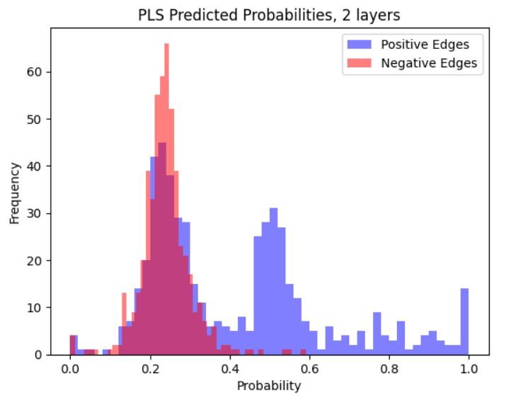
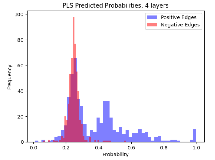
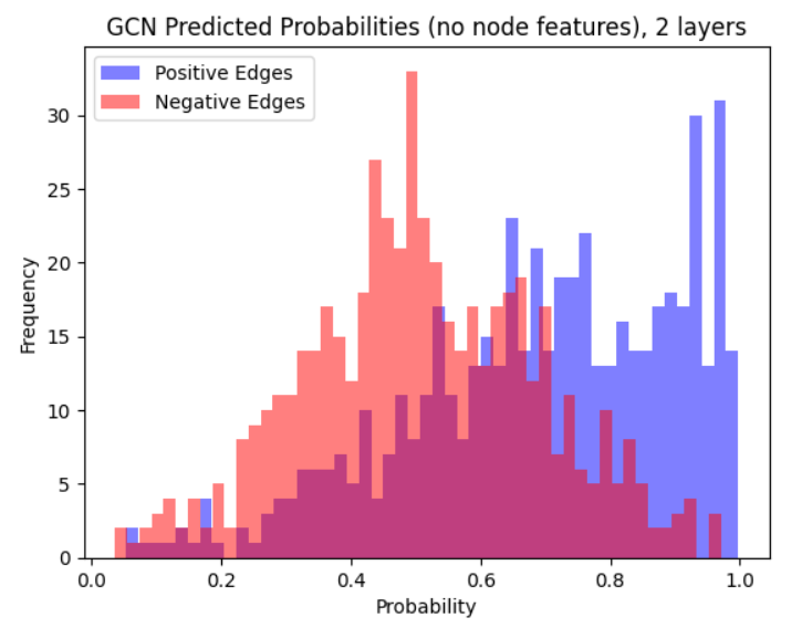
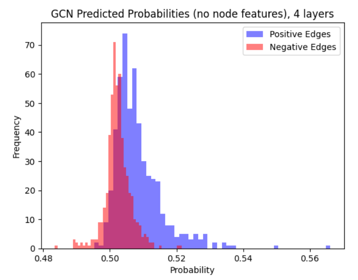
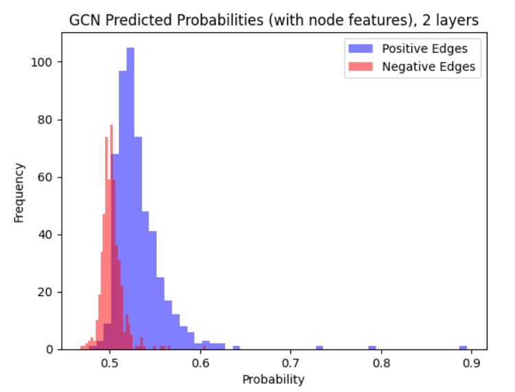
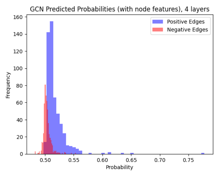
Appendix J Experiments (In-Sample)

J.1 6SSBM (80-20)

6-community symmetric stochastic block model with connection probabilities 0.8 and 0.2.

Table 9: Symmetric Stochastic Block Model with Connection Probabilities 0.8, 0.2
Cross Entropy Prob Ratio @ 100 Prob Ratio @ 500 AUC ROC
Parameters Model
rho=1, layers=2 GCN 0.587 ±\pm 0.010 1.000 ±\pm 0.000 1.000 ±\pm 0.000 0.697 ±\pm 0.002
LG-GNN 0.563 ±\pm 0.001 1.000 ±\pm 0.000 1.000 ±\pm 0.000 0.677 ±\pm 0.003
PLSG-GNN 0.583 ±\pm 0.004 1.000 ±\pm 0.000 1.000 ±\pm 0.000 0.673 ±\pm 0.004
rho=1, layers=4 GCN 0.693 ±\pm 0.000 0.973 ±\pm 0.009 0.978 ±\pm 0.006 0.640 ±\pm 0.029
LG-GNN 0.532 ±\pm 0.000 1.000 ±\pm 0.000 1.000 ±\pm 0.000 0.697 ±\pm 0.001
PLSG-GNN 0.579 ±\pm 0.002 1.000 ±\pm 0.000 0.999 ±\pm 0.001 0.680 ±\pm 0.002
rho=1/sqrt(n), layers=2 GCN 0.693 ±\pm 0.000 0.388 ±\pm 0.058 0.408 ±\pm 0.006 0.503 ±\pm 0.007
LG-GNN 0.090 ±\pm 0.001 0.458 ±\pm 0.035 0.450 ±\pm 0.006 0.503 ±\pm 0.007
PLSG-GNN 0.091 ±\pm 0.002 0.398 ±\pm 0.014 0.393 ±\pm 0.010 0.491 ±\pm 0.007
rho=1/sqrt(n), layers=4 GCN 0.693 ±\pm 0.000 0.383 ±\pm 0.009 0.376 ±\pm 0.004 0.499 ±\pm 0.007
LG-GNN 0.088 ±\pm 0.000 0.430 ±\pm 0.016 0.439 ±\pm 0.013 0.505 ±\pm 0.004
PLSG-GNN 0.089 ±\pm 0.001 0.388 ±\pm 0.009 0.388 ±\pm 0.012 0.507 ±\pm 0.001
rho=log(n)/n, layers=2 GCN 0.693 ±\pm 0.000 0.382 ±\pm 0.009 0.376 ±\pm 0.012 0.458 ±\pm 0.014
LG-GNN 0.021 ±\pm 0.001 0.367 ±\pm 0.004 0.389 ±\pm 0.002 0.517 ±\pm 0.006
PLSG-GNN 0.019 ±\pm 0.000 0.370 ±\pm 0.027 0.374 ±\pm 0.012 0.521 ±\pm 0.004
rho=log(n)/n, layers=4 GCN 0.693 ±\pm 0.000 0.405 ±\pm 0.007 0.380 ±\pm 0.005 0.496 ±\pm 0.010
LG-GNN 0.021 ±\pm 0.000 0.470 ±\pm 0.007 0.410 ±\pm 0.003 0.505 ±\pm 0.017
PLSG-GNN 0.019 ±\pm 0.000 0.380 ±\pm 0.004 0.375 ±\pm 0.007 0.513 ±\pm 0.010

J.2 6SSBM (55-45)

6-community symmetric stochastic block model with edge connection probabilities 0.55 and 0.45.

Table 10: Symmetric Stochastic Block Model with Connection Probabilities 0.55, 0.45
Cross Entropy Prob Ratio @ 100 Prob Ratio @ 500 AUC ROC
Parameters Model
rho=1, layers=2 GCN 0.693 ±\pm 0.000 0.859 ±\pm 0.004 0.852 ±\pm 0.001 0.500 ±\pm 0.001
LG-GNN 0.695 ±\pm 0.000 0.849 ±\pm 0.006 0.849 ±\pm 0.003 0.500 ±\pm 0.002
PLSG-GNN 0.693 ±\pm 0.000 0.849 ±\pm 0.006 0.849 ±\pm 0.003 0.500 ±\pm 0.002
rho=1, layers=4 GCN 0.693 ±\pm 0.000 0.847 ±\pm 0.000 0.846 ±\pm 0.003 0.500 ±\pm 0.000
LG-GNN 0.695 ±\pm 0.000 0.848 ±\pm 0.005 0.850 ±\pm 0.002 0.500 ±\pm 0.001
PLSG-GNN 0.693 ±\pm 0.000 0.853 ±\pm 0.005 0.851 ±\pm 0.002 0.501 ±\pm 0.001
rho=1/sqrt(n), layers=2 GCN 0.693 ±\pm 0.000 0.847 ±\pm 0.005 0.848 ±\pm 0.001 0.502 ±\pm 0.002
LG-GNN 0.130 ±\pm 0.000 0.852 ±\pm 0.001 0.849 ±\pm 0.000 0.503 ±\pm 0.006
PLSG-GNN 0.130 ±\pm 0.001 0.850 ±\pm 0.011 0.848 ±\pm 0.004 0.506 ±\pm 0.003
rho=1/sqrt(n), layers=4 GCN 0.693 ±\pm 0.000 0.848 ±\pm 0.002 0.847 ±\pm 0.002 0.502 ±\pm 0.006
LG-GNN 0.121 ±\pm 0.001 0.849 ±\pm 0.007 0.849 ±\pm 0.001 0.502 ±\pm 0.010
PLSG-GNN 0.131 ±\pm 0.001 0.848 ±\pm 0.005 0.852 ±\pm 0.002 0.495 ±\pm 0.004
rho=log(n)/n, layers=2 GCN 0.693 ±\pm 0.000 0.853 ±\pm 0.002 0.850 ±\pm 0.002 0.489 ±\pm 0.000
LG-GNN 0.031 ±\pm 0.000 0.845 ±\pm 0.007 0.850 ±\pm 0.003 0.508 ±\pm 0.008
PLSG-GNN 0.030 ±\pm 0.001 0.852 ±\pm 0.005 0.850 ±\pm 0.002 0.496 ±\pm 0.006
rho=log(n)/n, layers=4 GCN 0.693 ±\pm 0.000 0.851 ±\pm 0.004 0.848 ±\pm 0.002 0.487 ±\pm 0.004
LG-GNN 0.031 ±\pm 0.001 0.847 ±\pm 0.001 0.848 ±\pm 0.003 0.492 ±\pm 0.005
PLSG-GNN 0.030 ±\pm 0.001 0.856 ±\pm 0.007 0.852 ±\pm 0.003 0.508 ±\pm 0.017

J.3 10 SBM

10-community stochastic block model with parameter matrix PP that has randomly generated entries. The diagonal entries Pi,iP_{i,i} are generated as Unif(0.5,1)\text{Unif}(0.5,1), and Pi,jP_{i,j} is generated as Unif(0,min(Pi,i,Pj,j))\text{Unif}(0,\min(P_{i,i},P_{j,j})). The connection matrix is

(0.99490.30840.45530.37470.61870.00520.26260.57870.45400.67680.30840.83090.68510.05710.52250.33450.12790.01970.70630.77950.45530.68510.78540.10000.77260.18820.17360.67230.32780.60330.37470.05710.10000.61600.11680.09650.00210.18560.32480.45070.61870.52250.77260.11680.86140.54920.10980.42780.63860.11710.00520.33450.18820.09650.54920.66230.42770.00700.11450.28780.26260.12790.17360.00210.10980.42770.55280.20160.54660.04100.57870.01970.67230.18560.42780.00700.20160.88050.52330.07770.45400.70630.32780.32480.63860.11450.54660.52330.95100.48900.67680.77950.60330.45070.11710.28780.04100.07770.48900.8526)\begin{pmatrix}0.9949&0.3084&0.4553&0.3747&0.6187&0.0052&0.2626&0.5787&0.4540&0.6768\\ 0.3084&0.8309&0.6851&0.0571&0.5225&0.3345&0.1279&0.0197&0.7063&0.7795\\ 0.4553&0.6851&0.7854&0.1000&0.7726&0.1882&0.1736&0.6723&0.3278&0.6033\\ 0.3747&0.0571&0.1000&0.6160&0.1168&0.0965&0.0021&0.1856&0.3248&0.4507\\ 0.6187&0.5225&0.7726&0.1168&0.8614&0.5492&0.1098&0.4278&0.6386&0.1171\\ 0.0052&0.3345&0.1882&0.0965&0.5492&0.6623&0.4277&0.0070&0.1145&0.2878\\ 0.2626&0.1279&0.1736&0.0021&0.1098&0.4277&0.5528&0.2016&0.5466&0.0410\\ 0.5787&0.0197&0.6723&0.1856&0.4278&0.0070&0.2016&0.8805&0.5233&0.0777\\ 0.4540&0.7063&0.3278&0.3248&0.6386&0.1145&0.5466&0.5233&0.9510&0.4890\\ 0.6768&0.7795&0.6033&0.4507&0.1171&0.2878&0.0410&0.0777&0.4890&0.8526\\ \end{pmatrix}
Table 11: 10-community SBM with randomly generated parameters
Cross Entropy Prob Ratio @ 100 Prob Ratio @ 500 AUC ROC
Parameters Model
rho=1, layers=2 GCN 0.599 ±\pm 0.001 0.878 ±\pm 0.007 0.872 ±\pm 0.007 0.764 ±\pm 0.001
LG-GNN 0.588 ±\pm 0.001 0.908 ±\pm 0.008 0.867 ±\pm 0.009 0.726 ±\pm 0.002
PLSG-GNN 0.588 ±\pm 0.001 0.909 ±\pm 0.007 0.867 ±\pm 0.006 0.727 ±\pm 0.001
rho=1, layers=4 GCN 0.677 ±\pm 0.003 0.737 ±\pm 0.094 0.758 ±\pm 0.106 0.672 ±\pm 0.011
LG-GNN 0.562 ±\pm 0.008 0.868 ±\pm 0.042 0.868 ±\pm 0.037 0.780 ±\pm 0.002
PLSG-GNN 0.588 ±\pm 0.001 0.896 ±\pm 0.038 0.858 ±\pm 0.023 0.728 ±\pm 0.001
rho=1/sqrt(n), layers=2 GCN 0.693 ±\pm 0.000 0.288 ±\pm 0.022 0.315 ±\pm 0.008 0.505 ±\pm 0.003
LG-GNN 0.111 ±\pm 0.002 0.561 ±\pm 0.015 0.546 ±\pm 0.023 0.515 ±\pm 0.003
PLSG-GNN 0.110 ±\pm 0.001 0.610 ±\pm 0.008 0.577 ±\pm 0.005 0.520 ±\pm 0.005
rho=1/sqrt(n), layers=4 GCN 0.693 ±\pm 0.000 0.298 ±\pm 0.048 0.312 ±\pm 0.043 0.512 ±\pm 0.014
LG-GNN 0.105 ±\pm 0.003 0.584 ±\pm 0.036 0.564 ±\pm 0.011 0.516 ±\pm 0.008
PLSG-GNN 0.110 ±\pm 0.002 0.589 ±\pm 0.022 0.564 ±\pm 0.003 0.517 ±\pm 0.011
rho=log(n)/n, layers=2 GCN 0.693 ±\pm 0.000 0.300 ±\pm 0.017 0.307 ±\pm 0.014 0.478 ±\pm 0.019
LG-GNN 0.026 ±\pm 0.000 0.486 ±\pm 0.010 0.494 ±\pm 0.005 0.525 ±\pm 0.009
PLSG-GNN 0.024 ±\pm 0.000 0.493 ±\pm 0.012 0.490 ±\pm 0.004 0.514 ±\pm 0.018
rho=log(n)/n, layers=4 GCN 0.693 ±\pm 0.000 0.312 ±\pm 0.013 0.303 ±\pm 0.010 0.517 ±\pm 0.019
LG-GNN 0.026 ±\pm 0.002 0.498 ±\pm 0.004 0.494 ±\pm 0.007 0.517 ±\pm 0.014
PLSG-GNN 0.025 ±\pm 0.001 0.496 ±\pm 0.008 0.501 ±\pm 0.006 0.514 ±\pm 0.013

J.4 Geometric Graph

Each vertex ii has a latent feature XiX_{i} generated uniformly at random on 𝕊d1\mathbb{S}^{d-1}, d=11.d=11. Two vertices ii and jj are connected if Xi,Xjt=0.2,\langle X_{i},X_{j}\rangle\geq t=0.2, corresponding to a connection probability 0.26.\approx 0.26. Higher sparsity is achieved by adjusting tt.

Table 12: Geometric Graph with threshold 0.2 (corresponding to a connection probability of 0.26\approx 0.26)
Cross Entropy Prob Ratio @ 100 Prob Ratio @ 500 AUC ROC
Parameters Model
rho=1, layers=2 GCN 0.537 ±\pm 0.012 1.000 ±\pm 0.000 1.000 ±\pm 0.000 0.886 ±\pm 0.015
LG-GNN 0.354 ±\pm 0.005 1.000 ±\pm 0.000 1.000 ±\pm 0.000 0.916 ±\pm 0.004
PLSG-GNN 0.343 ±\pm 0.006 1.000 ±\pm 0.000 0.996 ±\pm 0.003 0.918 ±\pm 0.005
rho=1, layers=4 GCN 0.693 ±\pm 0.000 0.900 ±\pm 0.127 0.767 ±\pm 0.075 0.759 ±\pm 0.039
LG-GNN 0.305 ±\pm 0.002 1.000 ±\pm 0.000 1.000 ±\pm 0.000 0.950 ±\pm 0.002
PLSG-GNN 0.301 ±\pm 0.002 1.000 ±\pm 0.000 0.999 ±\pm 0.001 0.956 ±\pm 0.002
rho=1/sqrt(n), layers=2 GCN 0.693 ±\pm 0.000 0.333 ±\pm 0.062 0.232 ±\pm 0.030 0.848 ±\pm 0.007
LG-GNN 0.046 ±\pm 0.002 0.637 ±\pm 0.059 0.379 ±\pm 0.020 0.822 ±\pm 0.012
PLSG-GNN 0.046 ±\pm 0.002 0.453 ±\pm 0.076 0.293 ±\pm 0.035 0.844 ±\pm 0.012
rho=1/sqrt(n), layers=4 GCN 0.693 ±\pm 0.000 0.410 ±\pm 0.016 0.275 ±\pm 0.021 0.883 ±\pm 0.003
LG-GNN 0.045 ±\pm 0.001 0.637 ±\pm 0.054 0.377 ±\pm 0.024 0.827 ±\pm 0.003
PLSG-GNN 0.045 ±\pm 0.001 0.530 ±\pm 0.079 0.345 ±\pm 0.012 0.848 ±\pm 0.003
rho=log(n)/n, layers=2 GCN 0.693 ±\pm 0.000 0.003 ±\pm 0.005 0.019 ±\pm 0.005 0.624 ±\pm 0.018
LG-GNN 0.019 ±\pm 0.001 0.163 ±\pm 0.021 0.247 ±\pm 0.005 0.607 ±\pm 0.019
PLSG-GNN 0.019 ±\pm 0.000 0.100 ±\pm 0.024 0.097 ±\pm 0.014 0.611 ±\pm 0.009
rho=log(n)/n, layers=4 GCN 0.693 ±\pm 0.000 0.003 ±\pm 0.005 0.011 ±\pm 0.009 0.608 ±\pm 0.018
LG-GNN 0.019 ±\pm 0.001 0.170 ±\pm 0.022 0.237 ±\pm 0.029 0.609 ±\pm 0.032
PLSG-GNN 0.018 ±\pm 0.001 0.133 ±\pm 0.019 0.154 ±\pm 0.023 0.634 ±\pm 0.022

Appendix K Out-Sample Experiments

K.1 6SSBM (80-20)

6-community symmetric stochastic block model with connection probabilities 0.8 and 0.2.

Table 13: Symmetric Stochastic Block Model with Connection Probabilities 0.8, 0.2
Cross Entropy Prob Ratio @ 100 Prob Ratio @ 500 AUC ROC
Parameters Model
rho=1, layers=2 GCN 0.610 ±\pm 0.022 1.000 ±\pm 0.000 1.000 ±\pm 0.000 0.699 ±\pm 0.001
LG-GNN 0.569 ±\pm 0.004 0.998 ±\pm 0.004 0.998 ±\pm 0.001 0.682 ±\pm 0.002
PLSG-GNN 0.730 ±\pm 0.184 0.998 ±\pm 0.004 0.999 ±\pm 0.001 0.677 ±\pm 0.002
rho=1, layers=4 GCN 0.693 ±\pm 0.000 0.623 ±\pm 0.106 0.581 ±\pm 0.090 0.520 ±\pm 0.004
LG-GNN 0.545 ±\pm 0.004 1.000 ±\pm 0.000 1.000 ±\pm 0.000 0.698 ±\pm 0.001
PLSG-GNN 0.585 ±\pm 0.014 1.000 ±\pm 0.000 0.997 ±\pm 0.003 0.680 ±\pm 0.001
rho=1/sqrt(n), layers=2 GCN 0.693 ±\pm 0.000 0.448 ±\pm 0.028 0.423 ±\pm 0.005 0.502 ±\pm 0.008
LG-GNN 0.092 ±\pm 0.002 0.450 ±\pm 0.031 0.436 ±\pm 0.013 0.508 ±\pm 0.004
PLSG-GNN 0.091 ±\pm 0.002 0.405 ±\pm 0.004 0.387 ±\pm 0.003 0.503 ±\pm 0.003
rho=1/sqrt(n), layers=4 GCN 0.693 ±\pm 0.000 0.415 ±\pm 0.006 0.387 ±\pm 0.004 0.506 ±\pm 0.006
LG-GNN 0.088 ±\pm 0.002 0.460 ±\pm 0.011 0.436 ±\pm 0.008 0.501 ±\pm 0.014
PLSG-GNN 0.089 ±\pm 0.001 0.390 ±\pm 0.019 0.382 ±\pm 0.011 0.496 ±\pm 0.007
rho=log(n)/n, layers=2 GCN 0.693 ±\pm 0.000 0.382 ±\pm 0.018 0.371 ±\pm 0.008 0.488 ±\pm 0.010
LG-GNN 0.021 ±\pm 0.001 0.355 ±\pm 0.024 0.371 ±\pm 0.012 0.510 ±\pm 0.019
PLSG-GNN 0.019 ±\pm 0.001 0.387 ±\pm 0.049 0.377 ±\pm 0.015 0.491 ±\pm 0.030
rho=log(n)/n, layers=4 GCN 0.694 ±\pm 0.000 0.377 ±\pm 0.022 0.379 ±\pm 0.014 0.506 ±\pm 0.015
LG-GNN 0.021 ±\pm 0.000 0.460 ±\pm 0.054 0.384 ±\pm 0.011 0.499 ±\pm 0.015
PLSG-GNN 0.018 ±\pm 0.000 0.395 ±\pm 0.013 0.376 ±\pm 0.021 0.511 ±\pm 0.011

K.2 6SSBM (55-45)

6-community symmetric stochastic block model with edge connection probabilities 0.55 and 0.45.

Table 14: Symmetric Stochastic Block Model with Connection Probabilities 0.55, 0.45
Cross Entropy Prob Ratio @ 100 Prob Ratio @ 500 AUC ROC
Parameters Model
rho=1, layers=2 GCN 0.693 ±\pm 0.000 0.848 ±\pm 0.006 0.850 ±\pm 0.002 0.500 ±\pm 0.002
LG-GNN 0.698 ±\pm 0.002 0.845 ±\pm 0.005 0.846 ±\pm 0.003 0.500 ±\pm 0.001
PLSG-GNN 0.694 ±\pm 0.001 0.844 ±\pm 0.003 0.846 ±\pm 0.003 0.500 ±\pm 0.001
rho=1, layers=4 GCN 0.693 ±\pm 0.000 0.848 ±\pm 0.004 0.850 ±\pm 0.001 0.498 ±\pm 0.001
LG-GNN 0.702 ±\pm 0.001 0.847 ±\pm 0.012 0.848 ±\pm 0.004 0.499 ±\pm 0.001
PLSG-GNN 0.695 ±\pm 0.000 0.844 ±\pm 0.011 0.850 ±\pm 0.004 0.499 ±\pm 0.001
rho=1/sqrt(n), layers=2 GCN 0.693 ±\pm 0.000 0.851 ±\pm 0.004 0.850 ±\pm 0.002 0.496 ±\pm 0.004
LG-GNN 0.131 ±\pm 0.003 0.859 ±\pm 0.010 0.851 ±\pm 0.005 0.505 ±\pm 0.011
PLSG-GNN 0.131 ±\pm 0.002 0.844 ±\pm 0.007 0.850 ±\pm 0.001 0.505 ±\pm 0.003
rho=1/sqrt(n), layers=4 GCN 0.693 ±\pm 0.000 0.842 ±\pm 0.008 0.847 ±\pm 0.001 0.500 ±\pm 0.009
LG-GNN 0.123 ±\pm 0.001 0.850 ±\pm 0.003 0.849 ±\pm 0.001 0.497 ±\pm 0.016
PLSG-GNN 0.130 ±\pm 0.002 0.852 ±\pm 0.008 0.848 ±\pm 0.001 0.498 ±\pm 0.012
rho=log(n)/n, layers=2 GCN 0.693 ±\pm 0.000 0.844 ±\pm 0.007 0.850 ±\pm 0.001 0.488 ±\pm 0.031
LG-GNN 0.030 ±\pm 0.000 0.842 ±\pm 0.002 0.846 ±\pm 0.005 0.484 ±\pm 0.011
PLSG-GNN 0.029 ±\pm 0.001 0.851 ±\pm 0.001 0.849 ±\pm 0.002 0.505 ±\pm 0.008
rho=log(n)/n, layers=4 GCN 0.693 ±\pm 0.000 0.851 ±\pm 0.004 0.847 ±\pm 0.002 0.493 ±\pm 0.024
LG-GNN 0.030 ±\pm 0.002 0.844 ±\pm 0.005 0.845 ±\pm 0.003 0.488 ±\pm 0.015
PLSG-GNN 0.028 ±\pm 0.000 0.845 ±\pm 0.009 0.846 ±\pm 0.004 0.504 ±\pm 0.002

K.3 10 SBM

10-community stochastic block model with parameter matrix PP that has randomly generated entries. The diagonal entries Pi,iP_{i,i} are generated as Unif(0.5,1)\text{Unif}(0.5,1), and Pi,jP_{i,j} is generated as Unif(0,min(Pi,i,Pj,j))\text{Unif}(0,\min(P_{i,i},P_{j,j})). The connection matrix is

(0.99490.30840.45530.37470.61870.00520.26260.57870.45400.67680.30840.83090.68510.05710.52250.33450.12790.01970.70630.77950.45530.68510.78540.10000.77260.18820.17360.67230.32780.60330.37470.05710.10000.61600.11680.09650.00210.18560.32480.45070.61870.52250.77260.11680.86140.54920.10980.42780.63860.11710.00520.33450.18820.09650.54920.66230.42770.00700.11450.28780.26260.12790.17360.00210.10980.42770.55280.20160.54660.04100.57870.01970.67230.18560.42780.00700.20160.88050.52330.07770.45400.70630.32780.32480.63860.11450.54660.52330.95100.48900.67680.77950.60330.45070.11710.28780.04100.07770.48900.8526)\begin{pmatrix}0.9949&0.3084&0.4553&0.3747&0.6187&0.0052&0.2626&0.5787&0.4540&0.6768\\ 0.3084&0.8309&0.6851&0.0571&0.5225&0.3345&0.1279&0.0197&0.7063&0.7795\\ 0.4553&0.6851&0.7854&0.1000&0.7726&0.1882&0.1736&0.6723&0.3278&0.6033\\ 0.3747&0.0571&0.1000&0.6160&0.1168&0.0965&0.0021&0.1856&0.3248&0.4507\\ 0.6187&0.5225&0.7726&0.1168&0.8614&0.5492&0.1098&0.4278&0.6386&0.1171\\ 0.0052&0.3345&0.1882&0.0965&0.5492&0.6623&0.4277&0.0070&0.1145&0.2878\\ 0.2626&0.1279&0.1736&0.0021&0.1098&0.4277&0.5528&0.2016&0.5466&0.0410\\ 0.5787&0.0197&0.6723&0.1856&0.4278&0.0070&0.2016&0.8805&0.5233&0.0777\\ 0.4540&0.7063&0.3278&0.3248&0.6386&0.1145&0.5466&0.5233&0.9510&0.4890\\ 0.6768&0.7795&0.6033&0.4507&0.1171&0.2878&0.0410&0.0777&0.4890&0.8526\\ \end{pmatrix}
Table 15: 10-community SBM with randomly generated parameters
Cross Entropy Prob Ratio @ 100 Prob Ratio @ 500 AUC ROC
Parameters Model
rho=1, layers=2 GCN 0.635 ±\pm 0.014 0.709 ±\pm 0.125 0.726 ±\pm 0.108 0.716 ±\pm 0.019
LG-GNN 0.586 ±\pm 0.004 0.883 ±\pm 0.016 0.843 ±\pm 0.014 0.734 ±\pm 0.005
PLSG-GNN 0.586 ±\pm 0.004 0.886 ±\pm 0.016 0.844 ±\pm 0.013 0.735 ±\pm 0.005
rho=1, layers=4 GCN 0.801 ±\pm 0.193 0.645 ±\pm 0.025 0.633 ±\pm 0.027 0.578 ±\pm 0.109
LG-GNN 0.564 ±\pm 0.011 0.879 ±\pm 0.011 0.886 ±\pm 0.004 0.786 ±\pm 0.002
PLSG-GNN 0.592 ±\pm 0.004 0.883 ±\pm 0.013 0.836 ±\pm 0.015 0.732 ±\pm 0.001
rho=1/sqrt(n), layers=2 GCN 0.693 ±\pm 0.000 0.344 ±\pm 0.021 0.318 ±\pm 0.013 0.493 ±\pm 0.004
LG-GNN 0.115 ±\pm 0.002 0.580 ±\pm 0.020 0.557 ±\pm 0.007 0.497 ±\pm 0.009
PLSG-GNN 0.112 ±\pm 0.004 0.586 ±\pm 0.035 0.561 ±\pm 0.001 0.521 ±\pm 0.008
rho=1/sqrt(n), layers=4 GCN 0.693 ±\pm 0.000 0.285 ±\pm 0.016 0.275 ±\pm 0.006 0.486 ±\pm 0.006
LG-GNN 0.105 ±\pm 0.000 0.589 ±\pm 0.016 0.563 ±\pm 0.003 0.532 ±\pm 0.003
PLSG-GNN 0.111 ±\pm 0.002 0.578 ±\pm 0.013 0.544 ±\pm 0.009 0.508 ±\pm 0.011
rho=log(n)/n, layers=2 GCN 0.693 ±\pm 0.000 0.312 ±\pm 0.011 0.316 ±\pm 0.006 0.503 ±\pm 0.017
LG-GNN 0.026 ±\pm 0.000 0.528 ±\pm 0.029 0.504 ±\pm 0.006 0.506 ±\pm 0.015
PLSG-GNN 0.023 ±\pm 0.002 0.511 ±\pm 0.017 0.501 ±\pm 0.013 0.519 ±\pm 0.002
rho=log(n)/n, layers=4 GCN 0.693 ±\pm 0.000 0.304 ±\pm 0.027 0.304 ±\pm 0.015 0.518 ±\pm 0.005
LG-GNN 0.026 ±\pm 0.000 0.498 ±\pm 0.017 0.486 ±\pm 0.015 0.500 ±\pm 0.013
PLSG-GNN 0.024 ±\pm 0.000 0.546 ±\pm 0.018 0.505 ±\pm 0.018 0.498 ±\pm 0.016

K.4 Geometric Graph

We generate points uniformly on 𝕊d\mathbb{S}^{d} and connect two points if Xi,Xjt.\langle X_{i},X_{j}\rangle\geq t. For the following experiment, we chose d=11d=11 and t=0.3.t=0.3. This corresponds to a probability of about 0.15.

Table 16: Geometric Graph with threshold 0.2 (corresponding to a connection probability of 0.26\approx 0.26)
Cross Entropy Prob Ratio @ 100 Prob Ratio @ 500 AUC ROC
Parameters Model
rho=1, layers=2 GCN 0.573 ±\pm 0.015 1.000 ±\pm 0.000 0.996 ±\pm 0.002 0.873 ±\pm 0.020
LG-GNN 0.358 ±\pm 0.009 1.000 ±\pm 0.000 0.999 ±\pm 0.001 0.915 ±\pm 0.007
PLSG-GNN 0.350 ±\pm 0.013 0.997 ±\pm 0.005 0.999 ±\pm 0.002 0.917 ±\pm 0.010
rho=1, layers=4 GCN 0.693 ±\pm 0.000 0.813 ±\pm 0.021 0.733 ±\pm 0.079 0.591 ±\pm 0.016
LG-GNN 0.303 ±\pm 0.004 1.000 ±\pm 0.000 1.000 ±\pm 0.000 0.956 ±\pm 0.001
PLSG-GNN 0.298 ±\pm 0.004 1.000 ±\pm 0.000 1.000 ±\pm 0.000 0.958 ±\pm 0.001
rho=1/sqrt(n), layers=2 GCN 0.693 ±\pm 0.000 0.333 ±\pm 0.017 0.216 ±\pm 0.017 0.840 ±\pm 0.008
LG-GNN 0.046 ±\pm 0.003 0.523 ±\pm 0.037 0.311 ±\pm 0.021 0.818 ±\pm 0.022
PLSG-GNN 0.045 ±\pm 0.002 0.423 ±\pm 0.054 0.244 ±\pm 0.020 0.842 ±\pm 0.017
rho=1/sqrt(n), layers=4 GCN 0.693 ±\pm 0.000 0.313 ±\pm 0.021 0.207 ±\pm 0.013 0.848 ±\pm 0.021
LG-GNN 0.045 ±\pm 0.001 0.570 ±\pm 0.016 0.311 ±\pm 0.010 0.823 ±\pm 0.010
PLSG-GNN 0.045 ±\pm 0.001 0.510 ±\pm 0.014 0.289 ±\pm 0.003 0.843 ±\pm 0.013
rho=log(n)/n, layers=2 GCN 0.693 ±\pm 0.000 0.003 ±\pm 0.005 0.012 ±\pm 0.004 0.610 ±\pm 0.026
LG-GNN 0.018 ±\pm 0.000 0.210 ±\pm 0.029 0.276 ±\pm 0.005 0.616 ±\pm 0.018
PLSG-GNN 0.018 ±\pm 0.001 0.063 ±\pm 0.037 0.123 ±\pm 0.033 0.631 ±\pm 0.027
rho=log(n)/n, layers=4 GCN 0.693 ±\pm 0.000 0.007 ±\pm 0.009 0.035 ±\pm 0.007 0.607 ±\pm 0.002
LG-GNN 0.019 ±\pm 0.000 0.147 ±\pm 0.012 0.191 ±\pm 0.017 0.569 ±\pm 0.015
PLSG-GNN 0.018 ±\pm 0.000 0.107 ±\pm 0.012 0.143 ±\pm 0.018 0.607 ±\pm 0.010