This paper was converted on www.awesomepapers.org from LaTeX by an anonymous user.
Want to know more? Visit the Converter page.

Statistical and Computational Complexities of BFGS Quasi-Newton Method for Generalized Linear Models

Qiujiang Jin   Tongzheng Ren   Nhat Ho   Aryan Mokhtari Department of Electrical and Computer Engineering, UT Austin. {[email protected]}.Department of Computer Science, UT Austin. {[email protected]}.Department of Statistics and Data Sciences, UT Austin. {[email protected]}.Department of Electrical and Computer Engineering, UT Austin. {[email protected]}.
Abstract

The gradient descent (GD) method has been used widely to solve parameter estimation in generalized linear models (GLMs), a generalization of linear models when the link function can be non-linear. In GLMs with a polynomial link function, it has been shown that in the high signal-to-noise ratio (SNR) regime, due to the problem’s strong convexity and smoothness, GD converges linearly and reaches the final desired accuracy in a logarithmic number of iterations. In contrast, in the low SNR setting, where the problem becomes locally convex, GD converges at a slower rate and requires a polynomial number of iterations to reach the desired accuracy. Even though Newton’s method can be used to resolve the flat curvature of the loss functions in the low SNR case, its computational cost is prohibitive in high-dimensional settings as it is 𝒪(d3)\mathcal{O}(d^{3}), where dd the is the problem dimension. To address the shortcomings of GD and Newton’s method, we propose the use of the BFGS quasi-Newton method to solve parameter estimation of the GLMs, which has a per iteration cost of 𝒪(d2)\mathcal{O}(d^{2}). When the SNR is low, for GLMs with a polynomial link function of degree pp, we demonstrate that the iterates of BFGS converge linearly to the optimal solution of the population least-square loss function, and the contraction coefficient of the BFGS algorithm is comparable to that of Newton’s method. Moreover, the contraction factor of the linear rate is independent of problem parameters and only depends on the degree of the link function pp. Also, for the empirical loss with nn samples, we prove that in the low SNR setting of GLMs with a polynomial link function of degree pp, the iterates of BFGS reach a final statistical radius of 𝒪((d/n)12p+2)\mathcal{O}((d/n)^{\frac{1}{2p+2}}) after at most log(n/d)\log(n/d) iterations. This complexity is significantly less than the number required for GD, which scales polynomially with (n/d)(n/d).

1 Introduction

In supervised machine learning, we are given a set of nn independent samples denoted by X1,,XnX_{1},\dots,X_{n} with corresponding labels Y1,,YnY_{1},\dots,Y_{n}, that are drawn from some unknown distribution and our goal is to train a model that maps the feature vectors to their corresponding labels. We assume that the data is generated according to distribution 𝒫θ\mathcal{P}_{\theta^{*}} which is parameterized by a ground truth parameter θ\theta^{*}. Our goal as the learner is to find θ\theta^{*} by solving the empirical risk minimization (ERM) problem defined as

minθdn(θ):=1ni=1n(θ;(Xi,Yi)),\min_{\theta\in\mathbb{R}^{d}}\mathcal{L}_{n}(\theta):=\frac{1}{n}\sum_{i=1}^{n}\ell(\theta;(X_{i},Y_{i})), (1)

where (θ;(Xi,Yi))\ell(\theta;(X_{i},Y_{i})) is the loss function that measures the error between the predicted output of XiX_{i} using parameter θ\theta and its true label YiY_{i}. If we define θn\theta_{n}^{*} as an optimal solution of the above optimization problem, i.e., θnargminθdn(θ)\theta_{n}^{*}\in\arg\min_{\theta\in\mathbb{R}^{d}}\mathcal{L}_{n}(\theta), it can be considered as an approximation of the ground-truth solution θ\theta^{*}, where θ\theta^{*} is also a minimizer of the population loss defined as

minθd(θ):=𝔼[(θ;(X,Y))].\min_{\theta\in\mathbb{R}^{d}}\mathcal{L}(\theta):=\mathbb{E}\left[\ell(\theta;(X,Y))\right]. (2)

If one can solve the empirical risk efficiently, the output model could be close to θ\theta^{*}, when nn is sufficiently large. Several works have studied the complexity of iterative methods for solving ERM or directly the population loss, for the case that the objective function is convex or strongly convex with respect to θ\theta (Balakrishnan et al., 2017; Ho et al., 2020; Loh and Wainwright, 2015; Agarwal et al., 2012; Yuan and Zhang, 2013; Dwivedi et al., 2020b; Hardt et al., 2016; Candes et al., 2011). However, when we move beyond linear models, the underlying loss becomes non-convex and therefore the behavior of iterative methods could substantially change, and it is not even clear if they can reach a neighborhood of a global minimizer of the ERM problem.

The focus of this paper is on the generalized linear model (GLM) (Carroll et al., 1997; Netrapalli et al., 2015; Fienup, 1982; Shechtman et al., 2015; Feiyan Tian, 2021) where the labels and features are generated according to a polynomial link function and we have Yi=(Xiθ)p+ζiY_{i}=(X_{i}^{\top}\theta^{*})^{p}+\zeta_{i}, where ζi\zeta_{i} is an additive noise and p2p\geq 2 is an integer. Due to nonlinear structure of the generative model, even if we select a convex loss function \ell, the ERM problem denoted to the considered GLM could be non-convex with respect to θ\theta. Interestingly, depending on the norm of θ\theta^{*}, the curvature of the ERM problem and its corresponding population risk minimization problem could change substantially. More precisely, in the case that θ\|\theta^{*}\| is sufficiently large, which we refer to this case as the high signal-to-noise ratio (SNR) regime, the underlying population loss of the problem of interest is locally strongly convex and smooth. On the other hand, in the regime that θ\|\theta^{*}\| is close to zero, denoted by the low SNR regime, the underlying problem is neither strongly convex nor smooth, and in fact, it is ill-conditioned.

These observations lead to the conclusion that in the high SNR setting, due to strong convexity and smoothness of the underlying problem, gradient descent (GD) reaches the desired accuracy exponentially fast and overall it only requires logarithmic number of iterations. However, in the low SNR case, as the problem becomes locally convex, GD converges at a sublinear rate and thus requires polynomial number of iterations in terms of the sample size.

To address this issue, Ren et al. (2022a) advocated the use of GD with the Polyak step size to improve GD’s convergence in low SNR scenarios. hey demonstrated that the number of iterations could become logarithmic with respect to the sample size, when GD is deployed with the Polyak step size. However, such a method still remains a first-order algorithm and lacks any curvature approximation. Consequently, its overall complexity is directly proportional to the condition number of the problem. This, in turn, depends on both the condition number of the feature vectors’ covariance and the norm |θ||\theta^{*}|. As a result, in low SNR settings, the problem becomes ill-conditioned with a large condition number, and hence GD with the Polyak step size could be very slow. Furthermore, the implementation of the Polyak step size necessitates access to the optimal value of the objective function. As precise estimation of this optimal objective function value may not always be feasible, any inaccuracies could potentially lead to a reduced convergence rate for GD employing the Polyak step size.

Another alternative is to use a different distance metric instead of an adaptive step size to improve the convergence of GD for the low SNR setting. More precisely, Lu et al. (2018) have shown that the mirror descent method with a proper distance-generating function can solve the population loss corresponding to the low SNR setting at a linear rate. However, the linear convergence rate of mirror descent, similar to GD with Polyak step size, also depends on the condition number of the problem, and hence could lead to a slow convergence rate.

A natural approach to handle the ill-conditioning issue in the low SNR case as well as eliminating the need to estimate the optimal function value is the use of Newton’s method. As we show in this paper, this idea indeed addresses the issue of poor curvature of the problem and leads to an exponentially fast rate with contraction factor 2p22p1\frac{2p-2}{2p-1} in the population case, where pp is the degree of the polynomial link function. Moreover, in the high SNR setting, Newton’s method converges at a quadratic rate as the problem is strongly convex and smooth. Alas, these improvements come at the expense of increasing the computational complexity of each iteration to 𝒪(d3)\mathcal{O}(d^{3}) which is indeed more than the per iteration computational cost of GD that is 𝒪(d)\mathcal{O}(d). These points lead to this question:

Is there a computationally-efficient method that performs well in both high and low SNR settings at a reasonable per iteration computational cost?

Contributions. In this paper, we address this question and show that the BFGS method is capable of achieving these goals. BFGS is a quasi-Newton method that approximates the objective function curvature using gradient information and its per iteration cost is 𝒪(d2)\mathcal{O}(d^{2}). It is well-known that it enjoys a superlinear convergence rate that is independent of condition number in strongly convex and smooth settings, and hence, in the high SNR setting it outperforms GD. In the low SNR setting, where the Hessian at the optimal solution could be singular, we show that the BFGS method converges linearly and outperforms the sublinear convergence rate of GD. Next, we formally summarize our contributions.

  • Infinite sample, low SNR: For the infinite sample case where we minimize the population loss, we show that in the low SNR case the iterates of BFGS converge to the ground truth θ\theta^{*} at an exponentially fast rate that is independent of all problem parameters except the power of link function pp. We further show that the linear convergence contraction coefficient of BFGS is comparable to that of Newton’s method. This convergence result of BFGS is also of general interest as it provides the first global linear convergence of BFGS without line-search for a setting that is neither strictly nor strongly convex.

  • Finite sample, low SNR: By leveraging the results developed for the population loss of the low SNR regime, we show that in the finite sample case, the BFGS iterates converge to the final statistical radius 𝒪(1/n1/(2p+2))\mathcal{O}(1/n^{1/(2p+2)}) within the true parameter after a logarithmic number of iterations 𝒪(log(n))\mathcal{O}(\log(n)). It is substantially lower than the required number of iterations for fixed-step size GD, which is 𝒪(n(p1)/p)\mathcal{O}(n^{(p-1)/p}), to reach a similar statistical radius. This improvement is the direct outcome of the linear convergence of BFGS versus the sublinear convergence rate of GD in the low SNR case. Further, while the iteration complexity of BFGS is comparable to the logarithmic number of iterations of GD with Polyak step size, we show that BFGS removes the dependency of the overall complexity on the condition number of the problem as well as the need to estimate the optimal function value.

  • Experiments: We conduct numerical experiments for both infinite and finite sample cases to compare the performance of GD (with constant step size and Polyak step size), Newton’s method and BFGS. The provided empirical results are consistent with our theoretical findings and show the advantages of BFGS in the low SNR regime.

Outline. In Section 2, we discuss the BFGS quasi-Newton method. Section 3 details three scenarios in Generalized Linear Models (GLMs): low, middle, and high SNR regimes, outlining the characteristics of the population loss in each. Section 4 explores BFGS’s convergence in low SNR settings, highlighting its linear convergence rate, a marked improvement over gradient descent’s sublinear rate. This section also compares the convergence rates of BFGS and Newton’s method. Section 5 applies these insights to establish the convergence results of BFGS for the empirical loss n\mathcal{L}_{n} in the low SNR regime. Lastly, our numerical experiments are presented in Section 6.

2 BFGS algorithm

In this section, we review the basics of the BFGS quasi-Newton method, which is the main algorithm we analyze. Consider the case that we aim to minimize a differentiable convex function f:df:\mathbb{R}^{d}\to\mathbb{R}. The BFGS update is given by

θk+1=θkηkHkf(θk),k0,\theta_{k+1}=\theta_{k}-\eta_{k}H_{k}\nabla{f(\theta_{k})},\qquad\forall k\geq 0, (3)

where ηk\eta_{k} is the step size and Hkd×dH_{k}\in\mathbb{R}^{d\times d} is a positive definite matrix that aims to approximate the true Hessian inverse 2f(θk)1\nabla^{2}{f(\theta_{k})}^{-1}. There are several approaches for approximating HkH_{k} leading to different quasi-Newton methods, (Conn et al., 1991; Broyden, 1965; Broyden et al., 1973; Gay, 1979; Davidon, 1959; Fletcher and Powell, 1963; Broyden, 1970; Fletcher, 1970; Goldfarb, 1970; Shanno, 1970; Nocedal, 1980; Liu and Nocedal, 1989), but in this paper, we focus on the celebrated BFGS method, in which HkH_{k} is updated as

Hk=(Isk1uk1sk1uk1)Hk1(Iuk1sk1sk1uk1)+sk1sk1sk1uk1,k1,\begin{split}H_{k}=&\left(I-\frac{s_{k-1}u_{k-1}^{\top}}{s_{k-1}^{\top}u_{k-1}}\right)H_{k-1}\left(I-\frac{u_{k-1}s_{k-1}^{\top}}{s_{k-1}^{\top}u_{k-1}}\right)+\frac{s_{k-1}s_{k-1}^{\top}}{s_{k-1}^{\top}u_{k-1}},\qquad\forall k\geq 1,\end{split} (4)

where the variable variation sks_{k} and gradient displacement uku_{k} are defined as

sk1:=θkθk1,uk1:=f(θk)f(θk1),s_{k-1}:=\theta_{k}-\theta_{k-1},\qquad u_{k-1}:=\nabla{f(\theta_{k})}-\nabla{f(\theta_{k-1})}, (5)

for any k1k\geq 1 respectively. The logic behind the update in (4) is to ensure that the Hessian inverse approximation HkH_{k} satisfies the secant condition Hkuk1=sk1H_{k}u_{k-1}=s_{k-1}, while it stays close to the previous approximation matrix Hk1H_{k-1}. The update in (4) only requires matrix-vector multiplications, and hence, the computational cost per iteration of BFGS is 𝒪(d2)\mathcal{O}(d^{2}).

The main advantage of BFGS is its fast superlinear convergence rate under the assumption of strict convexity,

limkθkθoptθk1θopt=0,\lim_{k\to\infty}\frac{\|\theta_{k}-{\theta}_{opt}\|}{\|\theta_{k-1}-{\theta}_{opt}\|}=0,

where θopt{\theta}_{opt} is the optimal solution. Previous results on the superlinear convergence of quasi-Newton methods were all asymptotic, until the recent advancements on the non-asymptotic analysis of quasi-Newton methods (Rodomanov and Nesterov, 2021a, b, c; Jin and Mokhtari, 2020; Jin et al., 2022; Ye et al., 2021; Lin et al., 2021a, b). For instance, Jin and Mokhtari (2020) established a local superlinear convergence rate of (1/k)k(1/\sqrt{k})^{k} for BFGS. However, all these superlinear convergence analyses require the objective function to be smooth and strictly or strongly convex. Alas, these conditions are not satisfied in the low SNR setting, since the Hessian at the optimal solution could be singular, and hence the loss function is neither strongly convex nor strictly convex; we further discuss this point in Section 3. This observation implies that we need novel convergence analyses to study the behavior of BFGS in the low SNR setting, as we discuss in the upcoming sections.

3 Generalized linear model with polynomial link function

In this section, we formally present the generalized linear model (GLM) setting that we consider in our paper, and discuss the low and high SNR settings and optimization challenges corresponding to these cases. Consider the case that the feature vectors are denoted by XdX\in\mathbb{R}^{d} and their corresponding labels are denoted by YY\in\mathbb{R}. Suppose that we have access to nn sample points (Y1,X1),(Y2,X2),,(Yn,Xn)(Y_{1},X_{1}),(Y_{2},X_{2}),\ldots,(Y_{n},X_{n}) that are i.i.d. samples from the following generalized linear model with polynomial link function of power pp (Carroll et al., 1997), i.e.,

Yi=(Xiθ)p+ζi,\displaystyle Y_{i}=(X_{i}^{\top}\theta^{*})^{p}+\zeta_{i}, (6)

where θ\theta^{*} is a true but unknown parameter, pp\in\mathbb{N} is a given power, and ζ1,,ζn\zeta_{1},\ldots,\zeta_{n} are independent Gaussian noises with zero mean and variance σ2\sigma^{2}. The Gaussian assumption on the noise is for the simplicity of the discussion and similar results hold for the sub-Gaussian i.i.d. noise case. Furthermore, we assume the feature vectors are generated as X𝒩(0,Σ)X\sim\mathcal{N}(0,\Sigma) where Σd×d\Sigma\in\mathbb{R}^{d\times d} is a symmetric positive definite matrix. Here we focus on the settings that p+p\in\mathbb{N}^{+} and p2p\geq 2.

The above class of GLMs with polynomial link functions arise in several settings. When p=1p=1, the model in (6) is the standard linear regression model, and for the case that p=2p=2, the above setup corresponds to the phase retrieval model (Fienup, 1982; Shechtman et al., 2015; Candes et al., 2011; Netrapalli et al., 2015), which has found applications in optical imaging, x-ray tomography, and audio signal processing. Moreover, the analysis of GLMs with p2p\geq 2 also serves as the basis of the analysis on other popular statistical models. For example, as shown by Yi and Caramanis (2015); Wang et al. (2015); Xu et al. (2016); Balakrishnan et al. (2017); Daskalakis et al. (2017); Dwivedi et al. (2020a); Kwon et al. (2019); Dwivedi et al. (2020b); Kwon et al. (2021), the local landscape of log-likelihood for Gaussian mixture models and mixture linear regression models are identical to GLMs for p=2p=2.

In the case that the polynomial link function parameter in the GLM model in (6) is p=2p=2, by adapting similar arguments from Kwon et al. (2021) under the symmetric two-component location Gaussian mixture, there are essentially three regimes for estimating the true parameter θ\theta^{*}: Low signal-to-noise ratio (SNR) regime: θ/σC1(d/n)1/4\|\theta^{*}\|/\sigma\leq C_{1}(d/n)^{1/4} where dd is the dimension, nn is the sample size, and C1C_{1} is a universal constant; Middle SNR regime: C1(d/n)1/4θ/σCC_{1}(d/n)^{1/4}\!\leq\!\|\theta^{*}\|/\sigma\leq C where CC is a universal constant; High SNR regime: θ/σC\|\theta^{*}\|/\sigma\geq C. The main idea is that with different θ\theta^{*}, the optimization landscape of the parameter estimation problem changes. By generalizing the insights from the case p=2p=2, we define the following regimes for any p2p\geq 2:

  • (i) Low SNR regime: θ/σC1(d/n)1/(2p)\|\theta^{*}\|/\sigma\leq C_{1}(d/n)^{1/(2p)} where dd is the dimension, nn is the sample size, and C1C_{1} is a universal constant;

  • (ii) Middle SNR regime: C1(d/n)1/(2p)θ/σCC_{1}(d/n)^{1/(2p)}\!\leq\!\|\theta^{*}\|/\sigma\leq C where CC is a universal constant;

  • (iii) High SNR regime: θ/σC\|\theta^{*}\|/\sigma\geq C.

Note that, the rate (d/n)1/2p(d/n)^{1/2p} that we use to define the SNR regimes is from the statistical rate of estimating the true parameter θ\theta^{*} when θ\theta^{*} approaches 0. Next, we provide insight into the landscape of the least-square loss function for each regime. In particular, given the GLM in (6), the sample least-square takes the following form:

minθdn(θ):=1ni=1n(Yi(Xiθ)p)2.\min_{\theta\in\mathbb{R}^{d}}\mathcal{L}_{n}(\theta):=\frac{1}{n}\sum_{i=1}^{n}\left(Y_{i}-\left(X_{i}^{\top}\theta\right)^{p}\right)^{2}. (7)

To obtain insight about the landscape of the empirical loss function n\mathcal{L}_{n}, a useful approach is to consider that function by its population version, which we refer to as population least-square loss function:

minθd(θ):=𝔼[n(θ)],\min_{\theta\in\mathbb{R}^{d}}\mathcal{L}(\theta):=\mathbb{E}[\mathcal{L}_{n}(\theta)], (8)

where the outer expectation is taken with respect to the data.

High SNR regime. In the setting that the ground truth parameter has a relatively large norm, i.e., θC\|\theta^{*}\|\geq C for some constant C>0C>0 that only depends on σ\sigma, the population loss in (8) is locally strongly convex and smooth around θ\theta^{*}. More precisely, when θθ\|\theta-\theta^{*}\| is small, using Taylor’s theorem we have

(Xθ)p(Xθ)p=p(Xθ)p1X(θθ)+o(θθ).\displaystyle(X^{\top}\theta)^{p}-(X^{\top}\theta^{*})^{p}=p(X^{\top}\theta^{*})^{p-1}X^{\top}(\theta-\theta^{*})+o(\|\theta-\theta^{*}\|).

Hence, in a neighborhood of the optimal solution, the objective in (8) can be approximated as

(θ)=𝔼[(Y(Xθ)p)2]=𝔼[((Xθ)p+ζ(Xθ)p)2]=𝔼[((Xθ)p(Xθ)p)2]+𝔼[2ζ((Xθ)p(Xθ)p)2]+𝔼[ζ2]=𝔼[((Xθ)p(Xθ)p)2]+σ2=p2(θθ)𝔼X[X(Xθ)2p2X](θθ)+σ2+o(θθ2).\begin{split}\mathcal{L}(\theta)&=\mathbb{E}[(Y-(X^{\top}\theta)^{p})^{2}]=\mathbb{E}[((X^{\top}\theta^{*})^{p}+\zeta-(X^{\top}\theta)^{p})^{2}]\\ &=\mathbb{E}[((X^{\top}\theta^{*})^{p}-(X^{\top}\theta)^{p})^{2}]+\mathbb{E}[2\zeta((X^{\top}\theta^{*})^{p}-(X^{\top}\theta)^{p})^{2}]+\mathbb{E}[\zeta^{2}]\\ &=\mathbb{E}[((X^{\top}\theta^{*})^{p}-(X^{\top}\theta)^{p})^{2}]+\sigma^{2}\\ &=p^{2}(\theta-\theta^{*})^{\top}\mathbb{E}_{X}\left[X(X^{\top}\theta^{*})^{2p-2}X^{\top}\right](\theta-\theta^{*})+\sigma^{2}+o(\|\theta-\theta^{*}\|^{2}).\end{split}

Indeed, if θCσ\|\theta^{*}\|\geq C\sigma the above function behaves as a quadratic function that is smooth and strongly convex, assuming that o(θθ2)o(\|\theta-\theta^{*}\|^{2}) is negligible. As a result, the iterates of gradient descent (GD) converge to the solution at a linear rate and it requires κlog(1/ϵ)\kappa\log(1/\epsilon) to reach an ϵ\epsilon-accurate solution, where κ\kappa depends on the conditioning of the covariance matrix Σ\Sigma and the norm of θ\theta^{*}. In this case, BFGS converges superlinearly to θ\theta^{*} and the rate would be independent of κ\kappa, while the cost per iteration would be 𝒪(d2)\mathcal{O}(d^{2}).

Low SNR regime. As mentioned above, in the high SNR case, GD has a fast linear rate. However, in the low SNR case where θ\|\theta^{*}\| is small and θC1(d/n)1/(2p)\|\theta^{*}\|\leq C_{1}(d/n)^{1/(2p)}, the strong convexity parameter approaches zero when the sample size nn goes to infinity and the problem becomes ill-conditioned. In this case, we deal with a function that is only convex and its gradient is not Lipschitz continuous. To better elaborate on this point, let us focus on the case that θ=0\theta^{*}=0 as a special case of the low SNR setting. Considering the underlying distribution of XX, which is X𝒩(0,Σ)X\sim\mathcal{N}(0,\Sigma), for such a low SNR case, the population loss can be written as

(θ)=𝔼X[(Xθ)2p]+σ2=(2p1)!!Σ1/2θ2p+σ2.\mathcal{L}(\theta)=\mathbb{E}_{X}\left[(X^{\top}\theta)^{2p}\right]+\sigma^{2}=(2p-1)!!\|\Sigma^{1/2}\theta\|^{2p}+\sigma^{2}. (9)

Since we focus on p2p\geq 2 it can be verified that (θ)\mathcal{L}(\theta) is not strongly convex in a neighborhood of the solution θ=0\theta^{*}=0. For this class of functions, it is well-known that GD with constant step size would converge at a sublinear rate, and hence GD iterates require polynomial number of iterations to reach the final statistical radius. In the next section, we study the behavior of BFGS for solving the low SNR setting and showcase its advantage compared to GD.

Middle SNR regime. Different from the low and high SNR regimes, the middle SNR regime is generally harder to analyze as the landscapes of both the population and sample least-square loss functions are complex. Adapting the insight from middle SNR regime of the symmetric two-component location Gaussian mixtures from Kwon et al. (2021), for the middle SNR setting of the generalized linear model, the eigenvalues of the Hessian matrix of the population least-square loss function approach 0 and their vanishing rates depend on some increasing function of θ\|\theta^{*}\|. The optimal statistical rate of the optimization algorithms, such as gradient descent algorithm, for solving θ\theta^{*} depends strictly on the tightness of these vanishing rates in terms of θ\|\theta^{*}\|, which are non-trivial to obtain. In fact, to the best of our knowledge, there is no result on the convergence of iterative methods (such as GD or its variants) for GLMs with a polynomial link function in the middle SNR. Hence, we leave the study of BFGS for this setting as a future work.

4 Convergence analysis in the low SNR regime: Population loss

In this section, we focus on the convergence properties of BFGS for the population loss in the low SNR case introduced in (9). This analysis provides an intuition for the analysis of the finite sample case that we discuss in Section 5, as we expect these two loss functions to be close to each other when the number of samples nn is sufficiently large. In this section, instead of focusing on the population loss within the low SNR regime, as described in (9), we shift our attention to a more encompassing objective function, ff. Detailed in the following expression, this function encompasses the population loss function \mathcal{L} with θ=0\theta^{*}=0 as a specific example. This approach enables us to present our results in the most general setting possible. Specifically, we examine the function f:df:\mathbb{R}^{d}\rightarrow\mathbb{R}, defined as follows:

minθdf(θ)=Aθbq,\min_{\theta\in\mathbb{R}^{d}}f(\theta)=\|A\theta-b\|^{q}, (10)

where Am×dA\in\mathbb{R}^{m\times d} is a matrix, bmb\in\mathbb{R}^{m} is a given vector, and qq\in\mathbb{Z} satisfies q4q\geq 4. We should note that for q4q\geq 4, the considered objective is not strictly convex because the Hessian is singular when Aθ=bA\theta=b. Indeed, if we set m=dm=d and further let AA be Σ1/2\Sigma^{1/2} and choose b=Aθ=0b=A\theta^{*}=0, then we recover the problem in (9) for q=2pq=2p. Note that since we focus on the generalized linear model with the polynomial link function, which necessitates that pp be an integer, the parameter q=2pq=2p is also an integer.

Notice that the problem in (10), which serves as a surrogate for the finite sample problem that we plan to study in the next section, has the same solution set as the quadratic problem of minimizing Aθb2\|A\theta-b\|^{2} with solution (AA)1Ab(A^{\top}A)^{-1}A^{\top}b when AAA^{\top}A is invertible. Given this point, one might suggest that instead of minimizing (10) we could directly solve the quadratic problem which is indeed much easier to solve. This point is valid, but the goal of this section is not to efficiently solve problem (10) itself. Our goal is to understand the convergence properties of the BFGS method for solving the problem in (10) with the hope that it will provide some intuitions for the convergence analysis of BFGS for the empirical loss (7) in the low SNR regime. As we will discuss in Section 5, the convergence analysis of BFGS on the population loss which is a special case of (10) is closely related to the one for the empirical loss in (7).

Remark 1.

One remark is that population loss in (9) holds for the restrictive assumption of θ=0\theta^{*}=0, which is only a special case of the general low SNR regime of θC1(d/n)1/(2p)\|\theta^{*}\|\leq C_{1}(d/n)^{1/(2p)}. Our ultimate goal is to analyze the convergence behavior of the BFGS method applied to the empirical loss (7) of GLM problems in the low SNR regime. The errors between gradients and Hessians of the population loss with θ=0\theta^{*}=0 and θC1(d/n)1/(2p)\|\theta^{*}\|\leq C_{1}(d/n)^{1/(2p)} are upper bounded by the corresponding statistical errors between the population loss (8) and the empirical loss (7) in the low SNR regime, respectively. Therefore, the errors between iterations of applying BFGS to the population loss with θ=0\theta^{*}=0 and θC1(d/n)1/(2p)\|\theta^{*}\|\leq C_{1}(d/n)^{1/(2p)} are negligible compared to the statistical errors. Instead of directly analyzing BFGS for the population loss (8) in the general low SNR regime, studying the convergence properties of BFGS for the population loss (9) with θ=0\theta^{*}=0 can equivalently lay foundations for the convergence analysis of BFGS for the empirical loss (7) in the low SNR regime, which is the main target of this paper. The details can be found in Appendix A.4.

Our results in this section are of general interest from an optimization perspective, since there is no global convergence theory (without line-search) for the BFGS method in the literature when the objective function is not strictly convex. Our analysis provides one of the first results for such general settings. That said, it should be highlighted that our results do not hold for general convex problems, and we do utilize the specific structure of the considered convex problem to establish our results. The following examples illustrate some of the specific structures that we exploit to establish our result.

Assumption 1.

There exists θ^d\hat{\theta}\in\mathbb{R}^{d}, such that b=Aθ^b=A\hat{\theta}. In other words, bb is in the range of matrix AA.

This assumption implies that the problem in (10) is realizable, θ^\hat{\theta} is an optimal solution, and the optimal function value is zero. This assumption is satisfied in our considered low SNR setting in (9) as θ=0\theta^{*}=0 which implies b=0b=0.

Assumption 2.

The matrix AAd×dA^{\top}A\in\mathbb{R}^{d\times d} is invertible. This is equivalent to AA0A^{\top}A\succ 0.

The above assumption is also satisfied for our considered setting as we assume that the covariance matrix for our input features is positive definite. Combining Assumptions 1 and 2, we conclude that θ^\hat{\theta} is the unique optimal solution of problem (10). Next, we state the convergence rate of BFGS for solving problem (10) under the disclosed assumptions. The proof of the next theorem is available in Appendix A.1.

Theorem 1.

Consider the BFGS method in (3)-(5). Suppose Assumptions 1 and 2 hold, and the initial Hessian inverse approximation matrix is selected as H0=2f(θ0)1H_{0}=\nabla^{2}{f(\theta_{0})}^{-1}, where θ0d\theta_{0}\in\mathbb{R}^{d} is an arbitrary initial point. If the step size is ηk=1\eta_{k}=1 for all k0k\geq 0, then the iterates of BFGS converge to the optimal solution θ^\hat{\theta} at a linear rate of

θkθ^rk1θk1θ^,k1,\|\theta_{k}-\hat{\theta}\|\leq r_{k-1}\|\theta_{k-1}-\hat{\theta}\|,\quad\forall k\geq 1, (11)

where the contraction factors rk[0,1)r_{k}\in[0,1) satisfy

r0=q2q1,rk=1rk1q21rk1q1,k1.r_{0}=\frac{q-2}{q-1},\qquad r_{k}=\frac{1-r_{k-1}^{q-2}}{1-r_{k-1}^{q-1}},\quad\forall k\geq 1. (12)

Theorem 1 shows that the iterates of BFGS converge globally at a linear rate to the optimal solution of (10). This result is of interest as it illustrates the iterates generated by BFGS converge globally without any line search scheme and the step size is fixed as ηk=1\eta_{k}=1 for any k0k\geq 0. Moreover, the initial point θ0\theta_{0} is arbitrary and there is no restriction on the distance between θ0\theta_{0} and the optimal solution θ^\hat{\theta}.

We should highlight the above linear convergence result and our convergence analysis both rely heavily on the distinct structure of problem (10) and may not hold for a general convex minimization problem. Specifically, it can be shown that if we had access to the exact Hessian and could perform a Newton’s update to solve the problem in (10), then the error vectors (θkθ^)k0(\theta_{k}-\hat{\theta})_{k\geq 0} would all be parallel. This property arises due to the fact that for the problem in (10) the Newton direction is 2f(θk1)1f(θk1)=(θk1θ^)q2q1(θk1θ^)\nabla^{2}f(\theta_{k-1})^{-1}\nabla f(\theta_{k-1})=(\theta_{k-1}-\hat{\theta})-\frac{q-2}{q-1}(\theta_{k-1}-\hat{\theta}). Consequently, the next error vector θk1θ^\theta_{k-1}-\hat{\theta} computed by running one step of Newton would satisfy θkθ^=q2q1(θk1θ^)\theta_{k}-\hat{\theta}=\frac{q-2}{q-1}(\theta_{k-1}-\hat{\theta}). Therefore, the error vector at time kk, denoted by θkθ^\theta_{k}-\hat{\theta}, is parallel to the previous error vector θk1θ^\theta_{k-1}-\hat{\theta}, with the only difference being that its norm is reduced by a factor of q2q1\frac{q-2}{q-1}. Using an induction argument, it simply follows that all error vectors (θkθ^)k0(\theta_{k}-\hat{\theta})_{k\geq 0} remain parallel to each other while their norm contracts at a rate of q2q1\frac{q-2}{q-1}. This is a key point that is used in the result for Newton’s method in Theorem 3. In the convergence analysis of BFGS (stated in the proof of Theorem 1), we use a similar argument. While we cannot guarantee that the Hessian approximation matrix in the BFGS method matches the exact Hessian, we demonstrate that it can inherit this property, maintaining all error vectors (θkθ^)k0(\theta_{k}-\hat{\theta})_{k\geq 0} as parallel to each other. Additionally, we show that the norm is shrinking at a factor of rk<1r_{k}<1, which is always larger than q2q1\frac{q-2}{q-1}, yet remains independent of the problem’s condition number or dimensions. In the following theorem, we show that for q4q\geq 4, the linear rate contraction factors {rk}k=0\{r_{k}\}_{k=0}^{\infty} also converge linearly to a fixed point contraction factor rr_{*} determined by the parameter qq. The proof is available in Appendix A.2.
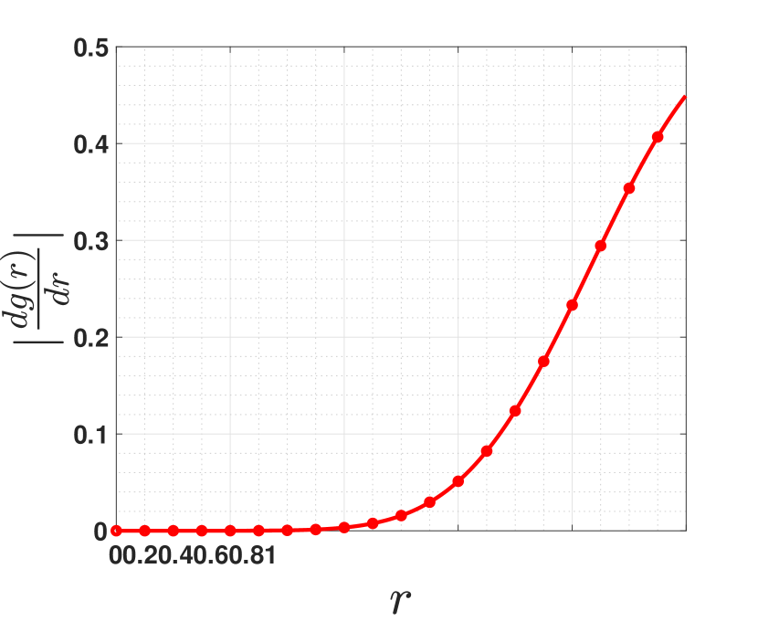
Theorem 2.

Consider the linear convergence factors {rk}k=0\{r_{k}\}_{k=0}^{\infty} defined in (12) from Theorem 1. If q4q\geq 4 and qq\in\mathbb{Z}, then the sequence {rk}k=0\{r_{k}\}_{k=0}^{\infty} converges to r(0,1)r_{*}\in(0,1) that is determined by the equation

rq1+rq2=1,r_{*}^{q-1}+r_{*}^{q-2}=1,\vspace{-0.5mm} (13)

and the rate of convergence is linear with a contraction factor that is at most 1/2{1}/{2}, i.e.,

|rkr|(1/2)k|r0r|,k0.|r_{k}-r_{*}|\leq\left({1}/{2}\right)^{k}|r_{0}-r_{*}|,\qquad\forall k\geq 0.\vspace{-0.5mm} (14)

Based on Theorem 2, the iterates of BFGS eventually converge to the optimal solution at the linear rate of rr_{*} determined by (13). Specifically, the factors {rk}k=0\{r_{k}\}_{k=0}^{\infty} converge to the fixed point rr_{*} at a linear rate with the contraction factor of 1/2{1}/{2}. Further, the linear convergence factors {rk}k=0\{r_{k}\}_{k=0}^{\infty} and their limit rr_{*} are all only determined by qq, and they are independent of the dimension dd and the condition number κA\kappa_{A} of the matrix AA. Hence, the performance of BFGS is not influenced by high-dimensional or ill-conditioned problems. This result is independently important from an optimization point of view, as it provides the first global linear convergence of BFGS without line-search for a setting that is not strictly or strongly convex, and interestingly the constant of linear convergence is independent of dimension or condition number.

Refer to caption
(a) q=4q=4.
Refer to caption
(b) q=100q=100.
Refer to caption
(c) q=4q=4.
Refer to caption
(d) q=100q=100.
Figure 1: Convergence of factors {rk}k=0\{r_{k}\}_{k=0}^{\infty} to rr_{*}.

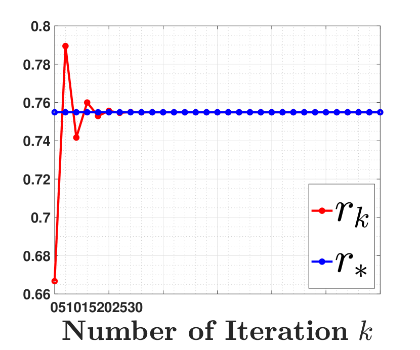
We illustrate the convergence of factors {rk}k=0\{r_{k}\}_{k=0}^{\infty} to the fixed point rr_{*} in Figure 1 for q=4q=4 and q=100q=100. In plots (a) and (b), we observe that rkr_{k} becomes close to rr_{*} after only 55 iterations. Hence, the linear convergence rate of BFGS is approximately rr_{*} after only a few iterations. We further observe in plots (c) and (d) that the factors {rk}k=0\{r_{k}\}_{k=0}^{\infty} converge to the fixed point rr_{*} at a linear rate upper bounded by 1/21/2. Note that rr_{*} is the solution of (13). These plots verify our results in Theorem 2.

Remark 2.

The cost of computing the initial Hessian inverse approximation H0=2f(θ0)1H_{0}=\nabla^{2}{f(\theta_{0})}^{-1} is 𝒪(d3)\mathcal{O}(d^{3}), but this cost is only required for the first iteration, and it is not required for k1k\geq 1 as for those iterates we update the Hessian inverse approximation matrix HkH_{k} based on the update in (4) at a cost of 𝒪(d2)\mathcal{O}(d^{2}).

Remark 3.

Although the vanilla Gradient Descent (GD) method converges at a sub-linear rate when applied to problem (10), it has been shown that other first-order methods, such as Mirror Descent with a distance-generating function h(x)=1q+2|x|q+2+12|x|2h(x)=\frac{1}{q+2}|x|^{q+2}+\frac{1}{2}|x|^{2} can solve problem (10) at a linear rate (refer to Lu et al. (2018)). However, the linear convergence rate of Mirror Descent is dependent on the condition number κ\kappa of the problem, characterized by the rate (11κ)\left(1-\frac{1}{\kappa}\right). In contrast, as demonstrated by Theorems 1 and 2, the linear convergence rate of BFGS is independent of the problem’s condition number. Consequently, in settings with low SNR, which can be ill-conditioned, we anticipate a faster convergence rate for BFGS compared to Mirror Descent. We illustrate this point in our numerical experiments presented in Figure 2.

4.1 Comparison with Newton’s method

Next, we compare the convergence results of BFGS for solving problem (10) with the one for Newton’s method. The following theorem characterizes the global linear convergence of Newton’s method with unit step size applied to the objective function in (10).

Theorem 3.

Consider applying Newton’s method to optimization problem (10) and suppose Assumptions 1 and 2 hold. Moreover, suppose the step size is ηk=1\eta_{k}=1 for any k0k\geq 0. Then, the iterates of Newton’s method converge to the optimal solution θ^\hat{\theta} at a linear rate of

θkθ^=q2q1θk1θ^,k1.\|\theta_{k}-\hat{\theta}\|=\frac{q-2}{q-1}\|\theta_{k-1}-\hat{\theta}\|,\quad\forall k\geq 1. (15)

Moreover, this linear convergence rate q2q1\frac{q-2}{q-1} is smaller than the fixed point rr_{*} defined in (13) of the BFGS quasi-Newton method, i.e., q2q1<r<2q32q2\frac{q-2}{q-1}<r_{*}<\frac{2q-3}{2q-2} for all q4q\geq 4.

The proof is available in Appendix A.3. The convergence results of Newton’s method are also global without any line search method, and the linear rate q2q1\frac{q-2}{q-1} is independent of dimension dd and condition number κA\kappa_{A}. Furthermore, the condition q2q1<r\frac{q-2}{q-1}<r_{*} implies that iterates of Newton’s method converge faster than BFGS, but the gap is not substantial as r<2q32q2r_{*}<\frac{2q-3}{2q-2}. On the other hand, the computational cost per iteration of Newton’s method is 𝒪(d3)\mathcal{O}(d^{3}) which is worse than the 𝒪(d2)\mathcal{O}(d^{2}) of BFGS.

Moving back to our main problem, one important implication of the above convergence results is that in the low SNR setting the iterates of BFGS converge linearly to the optimal solution of the population loss function, while the contraction coefficient of BFGS is comparable to that of Newton’s method which is (2p2)/(2p1)(2p-2)/(2p-1). For instance, for p=2,3,5,10p=2,3,5,10, the linear rate contraction factor of Newton’s method are 0.667,0.8,0.889,0.9470.667,0.8,0.889,0.947 and the approximate linear rate contraction factor of BFGS denoted by rr_{*} are 0.755,0.857,0.922,0.9630.755,0.857,0.922,0.963, respectively.

5 Convergence analysis in the low SNR regime: Finite sample setting

Thus far, we have demonstrated that the BFGS iterates converge linearly to the true parameter θ\theta^{*} when minimizing the population loss function \mathcal{L} of the GLM in (9) in the low SNR regime. In this section, we study the statistical behavior of the BFGS iterates for the finite sample case by leveraging the insights developed in the previous section about the convergence rate of BFGS in the infinite sample case, i.e., population loss. More precisely, we focus on the application of BFGS for solving the least-square loss function n\mathcal{L}_{n} defined in (7) for the low SNR setting. The iterates of BFGS in this case follow the update rule

θk+1n\displaystyle\theta_{k+1}^{n} =θknηkHknn(θkn),\displaystyle=\theta_{k}^{n}-\eta_{k}H_{k}^{n}\nabla\mathcal{L}_{n}(\theta_{k}^{n}), (16)

where HknH_{k}^{n} is updated using the gradient information of the loss n\mathcal{L}_{n} by the BFGS rule.

We next show that the BFGS iterates (16) {θkn}k0\{\theta_{k}^{n}\}_{k\geq 0} converge to the final statistical radius within a logarithmic number of iterations under the low SNR regime of the GLMs. To prove this claim, we track the difference between the iterates {θkn}k0\{\theta_{k}^{n}\}_{k\geq 0} generated based on the empirical loss and the iterates {θk}k0\{\theta_{k}\}_{k\geq 0} generated according to the population loss. Assuming that they both start from the same initialization θ0\theta_{0}, with the concentration of the gradient n(θ)(θ)\|\nabla\mathcal{L}_{n}(\theta)-\nabla\mathcal{L}(\theta)\| and the Hessian 2n(θ)2(θ)op\|\nabla^{2}\mathcal{L}_{n}(\theta)-\nabla^{2}\mathcal{L}(\theta)\|_{\mathrm{op}} from Mou et al. (2019); Ren et al. (2022b) we control the deviation between these two sequences. Using this bound and the convergence results of the iterates generated based on the population loss discussed in the previous section, we prove the following result for the finite sample setting. The proof is available in Appendix A.5.

Theorem 4.

Consider the low SNR regime of the GLM in (6) namely, θC1(d/n)1/(2p)\|\theta^{*}\|\leq C_{1}(d/n)^{1/(2p)}. Apply the BFGS method to the empirical loss (7) with the initial point θ0n\theta^{n}_{0}, where θ0n𝔹(θ,r)\theta^{n}_{0}\in\mathbb{B}(\theta^{*},r) for some r>0r>0, the initial Hessian inverse approximation matrix as H0=2n(θ0n)1H_{0}=\nabla^{2}{\mathcal{L}_{n}(\theta^{n}_{0})}^{-1}, where 2n(θ0n)\nabla^{2}{\mathcal{L}_{n}(\theta^{n}_{0})} is positive definite and step size ηk=1\eta_{k}=1. For any failure probability δ(0,1)\delta\in(0,1), if the number of samples is nC2(dlog(d/δ))2pn\geq C_{2}(d\log(d/\delta))^{2p}, and the number of iterations satisfies TC3log(n/d(log(1/δ)))T\geq C_{3}\log(n/d(\log(1/\delta))), then with probability 1δ1-\delta, we have

mint[T]θtnθC4(dlog(1/δ)n)12p+2,\min_{t\in[T]}\|\theta_{t}^{n}-\theta^{*}\|\leq C_{4}\left(\frac{d\log(1/\delta)}{n}\right)^{\frac{1}{2p+2}}, (17)

where C1C_{1}, C2C_{2}, C3C_{3}, and C4C_{4} are constants independent of nn and dd.

Our analysis hinges on linking the gradient and Hessian of the empirical loss to the population loss, subsequently demonstrating a convergence rate for the empirical loss based on the linear convergence established in Section 4 for the population loss. More details can be found in Appendix A.5. Theorem 4 shows that BFGS achieves an estimation accuracy of 𝒪((d/n)12p+2)\mathcal{O}((d/n)^{\frac{1}{2p+2}})in O(logn)O(\log n) iterations, which is substantialy faster than GD that requires O(np1p)O(n^{\frac{p-1}{p}}) iteations to achieve the same guarantee as shown in (Ren et al., 2022a). A few comments about Theorem 4 are in order.

Comparison to GD, GD with Polyak step size, and Newton’s method: Theorem 4 indicates that under the low SNR regime, the BFGS iterates reach the final statistical radius 𝒪(n1/(2p+2))\mathcal{O}(n^{-1/(2p+2)}) within the true parameter θ\theta^{*} after 𝒪(log(n))\mathcal{O}(\log(n)) number of iterations. The statistical radius is slightly worse than the optimal statistical radius O(n1/(2p))O(n^{-1/(2p)}). However, we conjecture that this is due to the proof technique and BFGS can still reach the optimal O(n1/(2p))O(n^{-1/(2p)}) in practice. In our experiments, in the next section, we observe that when d=4d=4 and p=2p=2, the statistical radius of BFGS is closer to the optimal radius of O(n1/4)O(n^{-1/4}) instead of O(n1/6)O(n^{-1/6}) suggested by our analysis. We leave an improvement of the statistical analysis as the future work. On the other hand, the overall iteration complexity of BFGS, which is 𝒪(log(n))\mathcal{O}(\log(n)), is indeed better than the polynomial number of iterations of GD, which is at the order of 𝒪(n(p1)/p)\mathcal{O}(n^{(p-1)/p}) (Corollary 3 in (Ho et al., 2020)).

Moreover, the complexity of BFGS is better than the one for GD with Polyak step size which is 𝒪(κlog(n))\mathcal{O}(\kappa\log(n)) iterations (Corollary 1 in (Ren et al., 2022a)), where κ\kappa is the condition number of the covariance matrix Σ\Sigma. Note that while the iteration complexity of BFGS is comparable to that of GD with Polyak step size in terms of the sample size, the BFGS overcomes the need to approximate the optimal value of the sample least-square loss n\mathcal{L}_{n}, which can be unstable in practice, and also removes the dependency on the condition number that appears in the complexity bound of GD with Polyak step size. A similar conclusion also holds for mirror descent with a distance-generating function h(x)=1q+2|x|q+2+12|x|2h(x)=\frac{1}{q+2}|x|^{q+2}+\frac{1}{2}|x|^{2}, as its linear convergence rate has a contraction factor of (11/κ)(1-1/\kappa), leading to an overall iteration complexity of 𝒪(κlog(n))\mathcal{O}(\kappa\log(n)).

Finally, the iteration complexity of BFGS is comparable to the 𝒪(log(n))\mathcal{O}(\log(n)) of Newton’s method (Corollary 3 in (Ho et al., 2020)), while per iteration cost of BFGS is substantially lower than Newton’s method.

On the minimum number of iterations: The results in Theorem 4 involve the minimum number of iterations, namely, this result holds for some 1tT1\leq t\leq T. It suggests that the BFGS iterates may diverge after they reach the final statistical radius. As highlighted in (Ho et al., 2020), such instability behavior of BFGS is inherent to fast and unstable methods. While it may sound limited, this issue can be handled via an early stopping scheme using the cross-validation approaches. We illustrate such early stopping of the BFGS iterates for the low SNR regime in Figure 3.

6 Numerical experiments

Our experiments are divided into two sections: the first focuses on iterative methods’ behavior on the population loss of GLMs with polynomial link functions, and the second examines the finite sample setting.

Refer to caption
(a) d=10,q=4d=10,q=4.
Refer to caption
(b) d=10,q=10d=10,q=10.
Refer to caption
(c) d=103,q=4d=10^{3},q=4.
Refer to caption
(d) d=103,q=10d=10^{3},q=10.
Figure 2: Convergence of Newton’s method, BFGS, GD with constant step size, GD with Polyak step size and mirror descent with constant step size for different values of dd and qq. In plot (a), m=100m=100 and η=104\eta=10^{-4}. In plot (b), m=100m=100 and η=108\eta=10^{-8}. In plot (c), m=2000m=2000 and η=1012\eta=10^{-12}. In plot (d), m=2000m=2000 and η=1015\eta=10^{-15}.

Experiments for the population loss function. In this section, we compare the performance of Newton’s method, BFGS, GD with constant step size, GD with Polyak step size, and and mirror descent with constant step size and distance generating function h(x)=1q+2xq+2+12x2h(x)=\frac{1}{q+2}\|x\|^{q+2}+\frac{1}{2}\|x\|^{2} applied to (10) which corresponds to the population loss. We choose different values of parameter mm, dimension dd and the exponential parameter qq in (10). We generate a random matrix Am×dA\in\mathbb{R}^{m\times d} and a random vector θ^d\hat{\theta}\in\mathbb{R}^{d}, and compute the vector b=Aθ^db=A\hat{\theta}\in\mathbb{R}^{d}. The initial point θ0d\theta_{0}\in\mathbb{R}^{d} is also generated randomly. To properly select the steps for GD with a fixed step size η\eta, we employed a manual grid search across the following values [1010,109,,101,1][10^{-10},10^{-9},...,10^{-1},1] and selected the value that yielded the best performance for each specific problem. In our plots, we present the logarithm of error θkθ^\|\theta_{k}-\hat{\theta}\| versus the number of iteration kk for different algorithms. All the values of different parameters mm, dd, qq and η\eta are mentioned in the caption of the plots.

Refer to caption
(a) High SNR regime.
Refer to caption
(b) Low SNR regime.
Refer to caption
(c) High SNR regime.
Refer to caption
(d) Low SNR regime.
Figure 3: Convergence of different methods when d=4d=4 in high SNR (a) and low SNR (b) regimes. Illustration of the statistical radius of BFGS in high SNR (c) and low SNR (d) regimes.

In Figure 2, we observe that GD with constant step converges slowly due to its sub-linear convergence rate. The performance of GD with Polyak step size is also poor when dimension is large or the parameter qq is huge. This is due to the fact that as dimension increases the problem becomes more ill-conditioned and hence the linear convergence contraction factor approaches 11. We observe that both Newton’s method and BFGS generate iterations with linear convergence rates, and their linear convergence rates are only affected by the parameter qq, i.e., the dimension dd has no impact over the performance of BFGS and Newton’s method. Although the convergence speed of Newton’s method is faster than BFGS, their gap is not significantly large as we expected from our theoretical results in Section 4. We also observe that mirror descent outperforms GD, but its performance is not as good as the BFGS method.

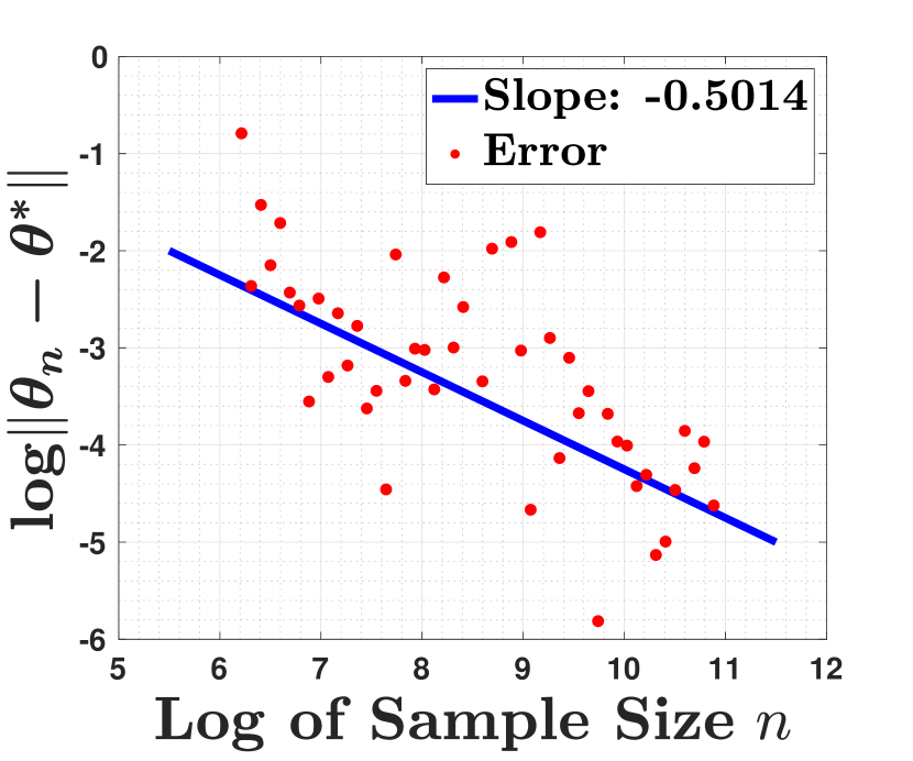
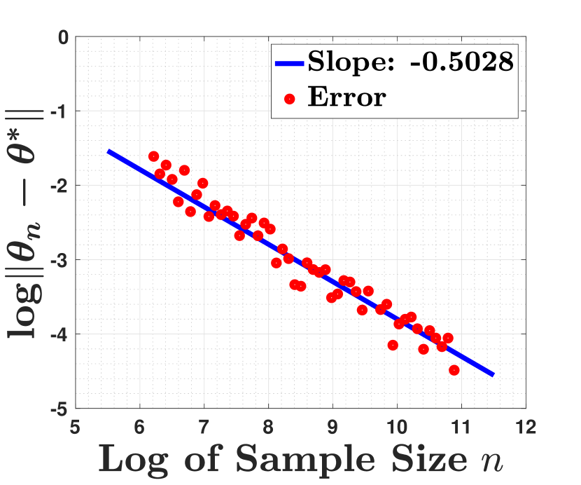
Experiments for the empirical loss function. We next study the statistical and computational complexities of BFGS on the empirical loss. In our experiments, we first consider the case that d=4d=4 and the power of the link function is p=2p=2, namely, we consider the multivariate setting of the phase retrieval problem. The data is generated by first sampling the inputs according to {Xi}i=1n𝒩(0,diag(σ12,,σ42))\{X_{i}\}_{i=1}^{n}\sim\mathcal{N}(0,\mathrm{diag}(\sigma_{1}^{2},\cdots,\sigma_{4}^{2})) where σk=(0.5)k1\sigma_{k}=(0.5)^{k-1}, and then generating their labels based on Yi=(Xiθ)2+ζiY_{i}=(X_{i}^{\top}\theta^{*})^{2}+\zeta_{i} where {ζi}i=1n\{\zeta_{i}\}_{i=1}^{n} are i.i.d. samples from 𝒩(0,0.01)\mathcal{N}(0,0.01). In the low SNR regime, we set θ=0\theta^{*}=0, and in the high SNR regime we select θ\theta^{*} uniformly at random from the unit sphere. Further, for GD, we set the step size as η=0.1\eta=0.1, while for Newton’s method and BFGS, we use the unit step size η=1\eta=1.

In plots (a) and (b) of Figure 3, we consider the setting that the sample size is n=104n=10^{4}, and we run GD, GD with Polyak step size, BFGS, and Newton’s method to find the optimal solution of the sample least-square loss n\mathcal{L}_{n}. Furthermore, for both Newton’s method and the BFGS algorithm, due to their instability, we also perform cross-validation to choose their early stopping. In particular, we split the data into training and the test sets. The training set consists of 90%90\% of the data while the test set has 10%10\% of the data. The yellow points in plots (a) and (b) of Figure 3 show the iterates of BFGS and Newton, respectively, with the minimum validation loss. As we observe, under the low SNR regime, the iterates of GD with Polyak step size, BFGS and Newton’s method converge geometrically fast to the final statistical radius while those of the GD converge slowly to that radius. Under the high SNR regime, the iterates of all of these methods converge geometrically fast to the final statistical radius. The faster convergence of GD with Polyak step size over GD is due to the optimal Polyak step size, while the faster convergence of BFGS and Newton’s method over GD is due to their independence on the problem condition number. Finally, in plots (c) and (d) of Figure 3, we run BFGS when the sample size is ranging from 10210^{2} to 10410^{4} to empirically verify the statistical radius of these methods. As indicated in the plots of that figure, under the high SNR regime, the BFGS has statistical radius is 𝒪(n1/2)\mathcal{O}(n^{-1/2}), while under the low SNR regime, its statistical radius becomes 𝒪(n1/4)\mathcal{O}(n^{-1/4}).

Refer to caption
(a) High SNR regime.
Refer to caption
(b) Low SNR regime.
Refer to caption
(c) High SNR regime.
Refer to caption
(d) Low SNR regime.
Figure 4: Convergence of different methods d=50d=50 in high SNR (a) and low SNR (b) regimes. Statistical radius of BFGS in high SNR (c) and low SNR (d) settings.
Refer to caption
(a) High SNR (d = 100).
Refer to caption
(b) Low SNR (d = 100).
Refer to caption
(c) High SNR (d = 500).
Refer to caption
(d) Low SNR (d = 500).
Figure 5: Convergence of different methods with d=100d=100 for high SNR regime are shown in (a) and low SNR regime in (b). Convergence of different methods with d=500d=500 for high SNR regime are shown in (c) and low SNR regime in (d).

To show that BFGS can also be applied to high dimension scenarios, we conduct additional experiments on the generalized linear model with input d=50,100,500d=50,100,500 and the power of link function p=2p=2. The inputs are generated by {Xi}i=1n𝒩(0,diag(σ12,,σd2))\{X_{i}\}_{i=1}^{n}\sim\mathcal{N}(0,\mathrm{diag}(\sigma_{1}^{2},\cdot,\sigma_{d}^{2})) where σk=(0.96)k1\sigma_{k}=(0.96)^{k-1}, and the remaining setting and hyper-parameters are set identical to the low dimension scenarios. The results are shown in Figure 4 and 5. As the results show, the performance of BFGS in high dimensional scenarios are nearly identical to the low dimensional scenarios.

7 Conclusions

In this paper, we analyzed the convergence rates of BFGS on both population and empirical loss functions of the generalized linear model in the low SNR regime. We showed that in this case, BFGS outperforms GD and performs similar to Newton’s method in terms of iteration complexity, while it requires a lower per iteration computational complexity compared to Newton’s method. We also provided experiments for both infinite and finite sample loss functions and showed that our empirical results are consistent with our theoretical findings. Perhaps one limitation of the BFGS method is that its computational cost is still not linear in the dimension and scales as 𝒪(d2)\mathcal{O}(d^{2}). One future research direction is to analyze some other iterative methods such as limited memory-BFGS (L-BFGS) which may be able to achieve a fast linear convergence rate in the low SNR setting, while its computational cost per iteration is 𝒪(d)\mathcal{O}(d).

References

  • Agarwal et al. (2012) A. Agarwal, S. Negahban, and M. J. Wainwright. Fast global convergence of gradient methods for high-dimensional statistical recovery. Annals of Statistics, 40(5):2452–2482, 2012.
  • Balakrishnan et al. (2017) S. Balakrishnan, M. J. Wainwright, and B. Yu. Statistical guarantees for the EM algorithm: From population to sample-based analysis. Annals of Statistics, 45:77–120, 2017.
  • Broyden et al. (1973) C. G. Broyden, J. E. Dennis Jr., Broyden, and J. J. More. On the local and superlinear convergence of quasi-Newton methods. IMA J. Appl. Math, 12(3):223–245, June 1973.
  • Broyden (1965) Charles G Broyden. A class of methods for solving nonlinear simultaneous equations. Mathematics of computation, 19(92):577–593, 1965.
  • Broyden (1970) Charles G Broyden. The convergence of single-rank quasi-Newton methods. Mathematics of Computation, 24(110):365–382, 1970.
  • Candes et al. (2011) Emmanuel J. Candes, Yonina Eldar, Thomas Strohmer, and Vlad Voroninski. Phase retrieval via matrix completion, 2011.
  • Carroll et al. (1997) R. J. Carroll, J. Fan, I. Gijbels, and M. P. Wand. Generalized partially linear single-index models. Journal of the American Statistical Association, 92:477–489, 1997.
  • Conn et al. (1991) Andrew R. Conn, Nicholas I. M. Gould, and Ph L Toint. Convergence of quasi-Newton matrices generated by the symmetric rank one update. Mathematical programming, 50(1-3):177–195, 1991.
  • Daskalakis et al. (2017) C. Daskalakis, C. Tzamos, and M. Zampetakis. Ten steps of EM suffice for mixtures of two Gaussians. In Proceedings of the 2017 Conference on Learning Theory, 2017.
  • Davidon (1959) WC Davidon. Variable metric method for minimization. Technical report, Argonne National Lab., Lemont, Ill., 1959.
  • Dwivedi et al. (2020a) R. Dwivedi, N. Ho, K. Khamaru, M. J. Wainwright, M. I. Jordan, and B. Yu. Sharp analysis of expectation-maximization for weakly identifiable models. AISTATS, 2020a.
  • Dwivedi et al. (2020b) R. Dwivedi, N. Ho, K. Khamaru, M. J. Wainwright, M. I. Jordan, and B. Yu. Singularity, misspecification, and the convergence rate of EM. Annals of Statistics, 44:2726–2755, 2020b.
  • Feiyan Tian (2021) Xiaoming Chen Feiyan Tian, Lei Liu. Generalized memory approximate message passing. https://arxiv.org/abs/2110.06069, 2021.
  • Fienup (1982) J. R. Fienup. Phase retrieval algorithms: a comparison. Appl. Opt., 21(15):2758–2769, Aug 1982. doi: 10.1364/AO.21.002758. URL http://www.osapublishing.org/ao/abstract.cfm?URI=ao-21-15-2758.
  • Fletcher (1970) Roger Fletcher. A new approach to variable metric algorithms. The computer journal, 13(3):317–322, 1970.
  • Fletcher and Powell (1963) Roger Fletcher and Michael JD Powell. A rapidly convergent descent method for minimization. The computer journal, 6(2):163–168, 1963.
  • Gay (1979) David M Gay. Some convergence properties of Broyden’s method. SIAM Journal on Numerical Analysis, 16(4):623–630, 1979.
  • Goebel and Kirk (1990) Kazimierz Goebel and W. A. Kirk. Topics in Metric Fixed Point Theory. Cambridge University Press, 1990.
  • Goldfarb (1970) Donald Goldfarb. A family of variable-metric methods derived by variational means. Mathematics of computation, 24(109):23–26, 1970.
  • Hardt et al. (2016) Moritz Hardt, Ben Recht, and Yoram Singer. Train faster, generalize better: Stability of stochastic gradient descent. In Maria Florina Balcan and Kilian Q. Weinberger, editors, Proceedings of The 33rd International Conference on Machine Learning, volume 48 of Proceedings of Machine Learning Research, pages 1225–1234, New York, New York, USA, 20–22 Jun 2016. PMLR. URL http://proceedings.mlr.press/v48/hardt16.html.
  • Ho et al. (2020) N. Ho, K. Khamaru, R. Dwivedi, M. J. Wainwright, M. I. Jordan, and B. Yu. Instability, computational efficiency and statistical accuracy. Arxiv Preprint Arxiv: 2005.11411, 2020.
  • Jin and Mokhtari (2020) Qiujiang Jin and Aryan Mokhtari. Non-asymptotic superlinear convergence of standard quasi-newton methods. arXiv preprint arXiv:2003.13607, 2020.
  • Jin et al. (2022) Qiujiang Jin, Alec Koppel, Ketan Rajawat, and Aryan Mokhtari. Sharpened quasi-newton methods: Faster superlinear rate and larger local convergence neighborhood. The 39th International Conference on Machine Learning (ICML 2022), 2022.
  • Kwon et al. (2019) J. Kwon, W. Qian, C. Caramanis, Y. Chen, , and D. Damek. Global convergence of the EM algorithm for mixtures of two component linear regression. In Conference on Learning Theory (COLT), 2019.
  • Kwon et al. (2021) J. Y. Kwon, N. Ho, and C. Caramanis. On the minimax optimality of the EM algorithm for learning two-component mixed linear regression. In AISTATS, 2021.
  • Lin et al. (2021a) Dachao Lin, Haishan Ye, and Zhihua Zhang. Explicit superlinear convergence of broyden’s method in nonlinear equations. arXiv preprint arXiv:2109.01974, 2021a.
  • Lin et al. (2021b) Dachao Lin, Haishan Ye, and Zhihua Zhang. Greedy and random quasi-newton methods with faster explicit superlinear convergence. Advances in Neural Information Processing Systems 34, 2021b.
  • Liu and Nocedal (1989) Dong C Liu and Jorge Nocedal. On the limited memory BFGS method for large scale optimization. Mathematical programming, 45(1-3):503–528, 1989.
  • Loh and Wainwright (2015) Po-Ling Loh and Martin J Wainwright. Regularized M-estimators with nonconvexity: Statistical and algorithmic theory for local optima. Journal of Machine Learning Research, 16:559–616, 2015.
  • Lu et al. (2018) Haihao Lu, Robert M Freund, and Yurii Nesterov. Relatively smooth convex optimization by first-order methods and applications. In SIAM Journal on Optimization, 28(1):333–354, 2018.
  • Mou et al. (2019) Wenlong Mou, Nhat Ho, Martin J Wainwright, Peter Bartlett, and Michael I Jordan. A diffusion process perspective on posterior contraction rates for parameters. arXiv preprint arXiv:1909.00966, 2019.
  • Netrapalli et al. (2015) Praneeth Netrapalli, Prateek Jain, and Sujay Sanghavi. Phase retrieval using alternating minimization. IEEE Transactions on Signal Processing, 63(18):4814–4826, 2015. doi: 10.1109/TSP.2015.2448516.
  • Nocedal (1980) Jorge Nocedal. Updating quasi-Newton matrices with limited storage. Mathematics of computation, 35(151):773–782, 1980.
  • Ren et al. (2022a) Tongzheng Ren, Fuheng Cui, Alexia Atsidakou, Sujay Sanghavi, and Nhat Ho. Towards statistical and computational complexities of Polyak step size gradient descent. Artificial Intelligence and Statistics Conference, 2022a.
  • Ren et al. (2022b) Tongzheng Ren, Jiacheng Zhuo, Sujay Sanghavi, and Nhat Ho. Improving computational complexity in statistical models with second-order information. arXiv preprint arXiv:2202.04219, 2022b.
  • Rodomanov and Nesterov (2021a) Anton Rodomanov and Yurii Nesterov. Greedy quasi-newton methods with explicit superlinear convergence. SIAM Journal on Optimization, 31(1):785–811, 2021a.
  • Rodomanov and Nesterov (2021b) Anton Rodomanov and Yurii Nesterov. Rates of superlinear convergence for classical quasi-newton methods. Mathematical Programming, pages 1–32, 2021b.
  • Rodomanov and Nesterov (2021c) Anton Rodomanov and Yurii Nesterov. New results on superlinear convergence of classical quasi-newton methods. Journal of Optimization Theory and Applications, 188(3):744–769, 2021c.
  • Shanno (1970) David F Shanno. Conditioning of quasi-Newton methods for function minimization. Mathematics of computation, 24(111):647–656, 1970.
  • Shechtman et al. (2015) Yoav Shechtman, Yonina C. Eldar, Oren Cohen, Henry Nicholas Chapman, Jianwei Miao, and Mordechai Segev. Phase retrieval with application to optical imaging: A contemporary overview. IEEE Signal Processing Magazine, 32(3):87–109, 2015. doi: 10.1109/MSP.2014.2352673.
  • Wang et al. (2015) Z. Wang, Q. Gu, Y. Ning, and H. Liu. High-dimensional expectation-maximization algorithm: Statistical optimization and asymptotic normality. In Advances in Neural Information Processing Systems 28, 2015.
  • Xu et al. (2016) J. Xu, D. Hsu, and A. Maleki. Global analysis of expectation maximization for mixtures of two Gaussians. In Advances in Neural Information Processing Systems 29, 2016.
  • Ye et al. (2021) Haishan Ye, Dachao Lin, Zhihua Zhang, and Xiangyu Chang. Explicit superlinear convergence rates of the sr1 algorithm. arXiv preprintarXiv:2105.07162, 2021.
  • Yi and Caramanis (2015) X. Yi and C. Caramanis. Regularized EM algorithms: A unified framework and statistical guarantees. In Advances in Neural Information Processing Systems 28, 2015.
  • Yuan and Zhang (2013) Xiao-Tong Yuan and Tong Zhang. Truncated power method for sparse eigenvalue problems. Journal of Machine Learning Research, 14(Apr):899–925, 2013.

Appendix

Appendix A Proofs

Lemma 1.

Consider the objective function in (10) satisfying Assumption 1 and 2. Then, the inverse matrix of its Hessian 2f(θ)\nabla^{2}{f(\theta)} can be expressed as

2f(θ)1=(AA)1qAθbq2(q2)(θθ^)(θθ^)q(q1)Aθbq.\nabla^{2}{f(\theta)}^{-1}=\frac{(A^{\top}A)^{-1}}{q\|A\theta-b\|^{q-2}}-\frac{(q-2)(\theta-\hat{\theta})(\theta-\hat{\theta})^{\top}}{q(q-1)\|A\theta-b\|^{q}}. (18)
Proof.

Notice that the Hessian of objective function (10) can be expressed as

2f(θ)=qAθbq2AA+q(q2)Aθbq4A(Aθb)(Aθb)A.\nabla^{2}{f(\theta)}=q\|A\theta-b\|^{q-2}A^{\top}A+q(q-2)\|A\theta-b\|^{q-4}A^{\top}(A\theta-b)(A\theta-b)^{\top}A. (19)

We use the Sherman–Morrison formula. Suppose that Xd×dX\in\mathbb{R}^{d\times d} is an invertible matrix and a,bda,b\in\mathbb{R}^{d} are two vectors satisfying that 1+bX1a01+b^{\top}X^{-1}a\neq 0. Then, the matrix X+abX+ab^{\top} is invertible and

(X+ab)1=X1X1abX11+bX1a.(X+ab^{\top})^{-1}=X^{-1}-\frac{X^{-1}ab^{\top}X^{-1}}{1+b^{\top}X^{-1}a}.

Applying the Sherman–Morrison formula with X=qAθbq2AAX=q\|A\theta-b\|^{q-2}A^{\top}A, a=q(q2)Aθbq4A(Aθb)a=q(q-2)\|A\theta-b\|^{q-4}A^{\top}(A\theta-b) and b=A(Aθb)b=A^{\top}(A\theta-b). Notice that AAA^{\top}A is invertible, hence XX is invertible and

1+bX1a=1+(Aθb)A(AA)1qAθbq2q(q2)Aθbq4A(Aθb)=1+(q2)(Aθb)A(AA)1AA(θθ^)Aθb2=1+(q2)(Aθb)(Aθb)Aθb2=q10.(Since q4.)\begin{split}&1+b^{\top}X^{-1}a\\ =&\quad 1+(A\theta-b)^{\top}A\frac{(A^{\top}A)^{-1}}{q\|A\theta-b\|^{q-2}}q(q-2)\|A\theta-b\|^{q-4}A^{\top}(A\theta-b)\\ =&\quad 1+(q-2)(A\theta-b)^{\top}A\frac{(A^{\top}A)^{-1}A^{\top}A(\theta-\hat{\theta})}{\|A\theta-b\|^{2}}\\ =&\quad 1+(q-2)\frac{(A\theta-b)^{\top}(A\theta-b)}{{\|A\theta-b\|^{2}}}\\ =&\quad q-1\neq 0.\qquad\text{(Since $q\geq 4$.)}\end{split}

Therefore, we obtain that

2f(θ)1=(AA)1qAθbq2(AA)1qAθbq2q(q2)Aθbq4A(Aθb)(A(Aθb))(AA)1qAθbq2q1=(AA)1qAθbq2(q2)q(q1)Aθbq(AA)1AA(θθ^)(θθ^)AA(AA)1=(AA)1qAθbq2(q2)(θθ^)(θθ^)q(q1)Aθbq.\begin{split}&\nabla^{2}{f(\theta)}^{-1}\\ =&\quad\frac{(A^{\top}A)^{-1}}{q\|A\theta-b\|^{q-2}}-\frac{\frac{(A^{\top}A)^{-1}}{q\|A\theta-b\|^{q-2}}q(q-2)\|A\theta-b\|^{q-4}A^{\top}(A\theta-b)(A^{\top}(A\theta-b))^{\top}\frac{(A^{\top}A)^{-1}}{q\|A\theta-b\|^{q-2}}}{q-1}\\ =&\quad\frac{(A^{\top}A)^{-1}}{q\|A\theta-b\|^{q-2}}-\frac{(q-2)}{q(q-1)\|A\theta-b\|^{q}}(A^{\top}A)^{-1}AA^{\top}(\theta-\hat{\theta})(\theta-\hat{\theta})^{\top}AA^{\top}(A^{\top}A)^{-1}\\ =&\quad\frac{(A^{\top}A)^{-1}}{q\|A\theta-b\|^{q-2}}-\frac{(q-2)(\theta-\hat{\theta})(\theta-\hat{\theta})^{\top}}{q(q-1)\|A\theta-b\|^{q}}.\end{split} (20)

As a consequence, we obtain the conclusion of the lemma. ∎

Lemma 2.

Banach’s Fixed-Point Theorem. Consider the differentiable function f:DDf:D\subset\mathbb{R}\to D\subset\mathbb{R}. Suppose that there exists C(0,1)C\in(0,1) such that |f(x)|C|f^{\prime}(x)|\leq C for any xDx\in D. Now let x0Dx_{0}\in D be arbitrary and define the sequence {xk}k=0\{x_{k}\}_{k=0}^{\infty} as

xk+1=f(xk),k0.x_{k+1}=f(x_{k}),\qquad\forall k\geq 0. (21)

Then, the sequence {xk}k=0\{x_{k}\}_{k=0}^{\infty} converges to the unique fixed point xx_{*} defined as

x=f(x),x_{*}=f(x_{*}), (22)

with linear convergence rate of

|xkx|Ck|x0x|,k0.|x_{k}-x_{*}|\leq C^{k}|x_{0}-x_{*}|,\qquad\forall k\geq 0. (23)
Proof.

Check [Goebel and Kirk, 1990]. ∎

A.1 Proof of Theorem 1

We use induction to prove the convergence results in (11) and (12). Note that b=Aθ^b=A\hat{\theta} by Assumption 1 and the gradient and Hessian of the objective function in (10) are explicitly given by

f(θ)=qAθbq2A(Aθb)=qAθbq2AA(θθ^),\nabla{f(\theta)}=q\|A\theta-b\|^{q-2}A^{\top}(A\theta-b)=q\|A\theta-b\|^{q-2}A^{\top}A(\theta-\hat{\theta}), (24)
2f(θ)=qAθbq2AA+q(q2)Aθbq4A(Aθb)(Aθb)A.\nabla^{2}{f(\theta)}=q\|A\theta-b\|^{q-2}A^{\top}A+q(q-2)\|A\theta-b\|^{q-4}A^{\top}(A\theta-b)(A\theta-b)^{\top}A. (25)

Applying Lemma 1, we can obtain that

2f(θ)1=(AA)1qAθbq2(q2)(θθ^)(θθ^)q(q1)Aθbq.\nabla^{2}{f(\theta)}^{-1}=\frac{(A^{\top}A)^{-1}}{q\|A\theta-b\|^{q-2}}-\frac{(q-2)(\theta-\hat{\theta})(\theta-\hat{\theta})^{\top}}{q(q-1)\|A\theta-b\|^{q}}. (26)

First, we consider the initial iteration

θ1=θ0H0f(θ0)=θ0f(θ0)1f(θ0),\theta_{1}=\theta_{0}-H_{0}\nabla{f(\theta_{0})}=\theta_{0}-\nabla{f(\theta_{0})}^{-1}\nabla{f(\theta_{0})},
θ1θ^=θ0θ^f(θ0)1f(θ0).\theta_{1}-\hat{\theta}=\theta_{0}-\hat{\theta}-\nabla{f(\theta_{0})}^{-1}\nabla{f(\theta_{0})}.

Notice that b=Aθ^b=A\hat{\theta} by Assumption 1 and

2f(θ0)1f(θ0)=[(AA)1qAθ0bq2(q2)(θ0θ^)(θ0θ^)q(q1)Aθ0bq]qAθbq2AA(θ0θ^)=θ0θ^q2q1(θ0θ^)AA(θ0θ^)Aθ0b2(θ0θ^)=θ0θ^q2q1(Aθ0b)(Aθ0b)Aθ0b2(θ0θ^)=θ0θ^q2q1(θ0θ^).\begin{split}&\nabla^{2}{f(\theta_{0})}^{-1}\nabla{f(\theta_{0})}\\ =&\quad\left[\frac{(A^{\top}A)^{-1}}{q\|A\theta_{0}-b\|^{q-2}}-\frac{(q-2)(\theta_{0}-\hat{\theta})(\theta_{0}-\hat{\theta})^{\top}}{q(q-1)\|A\theta_{0}-b\|^{q}}\right]q\|A\theta-b\|^{q-2}A^{\top}A(\theta_{0}-\hat{\theta})\\ =&\quad\theta_{0}-\hat{\theta}-\frac{q-2}{q-1}\frac{(\theta_{0}-\hat{\theta})^{\top}A^{\top}A(\theta_{0}-\hat{\theta})}{\|A\theta_{0}-b\|^{2}}(\theta_{0}-\hat{\theta})\\ =&\quad\theta_{0}-\hat{\theta}-\frac{q-2}{q-1}\frac{(A\theta_{0}-b)^{\top}(A\theta_{0}-b)}{\|A\theta_{0}-b\|^{2}}(\theta_{0}-\hat{\theta})\\ =&\quad\theta_{0}-\hat{\theta}-\frac{q-2}{q-1}(\theta_{0}-\hat{\theta}).\end{split} (27)

Therefore, we obtain that

θ1θ^=θ0θ^f(θ0)1f(θ0)=q2q1(θ0θ^).\theta_{1}-\hat{\theta}=\theta_{0}-\hat{\theta}-\nabla{f(\theta_{0})}^{-1}\nabla{f(\theta_{0})}=\frac{q-2}{q-1}(\theta_{0}-\hat{\theta}).

Condition (11) holds for k=1k=1 with r0=q2q1r_{0}=\frac{q-2}{q-1}. Now we assume that condition (11) holds for k=tk=t where t1t\geq 1, i.e.,

θtθ^=rt1(θt1θ^).\theta_{t}-\hat{\theta}=r_{t-1}(\theta_{t-1}-\hat{\theta}). (28)

Considering the condition b=Aθ^b=A\hat{\theta} in Assumption 1 and the condition in (28), we further have

Aθtb=A(θtθ^)=rt1A(θt1θ^)=rt1(Aθt1b),A\theta_{t}-b=A(\theta_{t}-\hat{\theta})=r_{t-1}A(\theta_{t-1}-\hat{\theta})=r_{t-1}(A\theta_{t-1}-b),

which implies that

f(θt)=qrt1q1A(θt1θ^)q2AA(θt1θ^).\nabla{f(\theta_{t})}=qr_{t-1}^{q-1}\|A(\theta_{t-1}-\hat{\theta})\|^{q-2}A^{\top}A(\theta_{t-1}-\hat{\theta}). (29)

We further show that the variable displacement and gradient difference can be written as

st1=θtθt1=θtθ^θt1+θ^=(rt11)(θt1θ^),s_{t-1}=\theta_{t}-\theta_{t-1}=\theta_{t}-\hat{\theta}-\theta_{t-1}+\hat{\theta}=(r_{t-1}-1)(\theta_{t-1}-\hat{\theta}),

and

ut1=f(θt)f(θt1)=q(rt1q11)A(θt1θ^)q2AA(θt1θ^).u_{t-1}=\nabla{f(\theta_{t})}-\nabla{f(\theta_{t-1})}=q(r_{t-1}^{q-1}-1)\|A(\theta_{t-1}-\hat{\theta})\|^{q-2}A^{\top}A(\theta_{t-1}-\hat{\theta}).

Considering these expressions, we can show that the rank-1 matrix in the update of BFGS ut1st1u_{t-1}s_{t-1}^{\top} is given by

ut1st1=q(rt1q11)(rt11)A(θt1θ^)q2AA(θt1θ^)(θt1θ^),u_{t-1}s_{t-1}^{\top}=q(r_{t-1}^{q-1}-1)(r_{t-1}-1)\|A(\theta_{t-1}-\hat{\theta})\|^{q-2}A^{\top}A(\theta_{t-1}-\hat{\theta})(\theta_{t-1}-\hat{\theta})^{\top},

and the inner product st1ut1s_{t-1}^{\top}u_{t-1} can be written as

st1ut1=q(rt1q11)(rt11)A(θt1θ^)q2(θt1θ^)AA(θt1θ^)=q(rt1q11)(rt11)A(θt1θ^)q.\begin{split}s_{t-1}^{\top}u_{t-1}&=q(r_{t-1}^{q-1}-1)(r_{t-1}-1)\|A(\theta_{t-1}-\hat{\theta})\|^{q-2}(\theta_{t-1}-\hat{\theta})^{\top}A^{\top}A(\theta_{t-1}-\hat{\theta})\\ &=q(r_{t-1}^{q-1}-1)(r_{t-1}-1)\|A(\theta_{t-1}-\hat{\theta})\|^{q}.\end{split}

These two expressions allow us to simplify the matrix Iut1st1st1ut1I-\frac{u_{t-1}s_{t-1}^{\top}}{s_{t-1}^{\top}u_{t-1}} in the update of BFGS as

Iut1st1st1ut1=IAA(θt1θ^)(θt1θ^)A(θt1θ^)2.I-\frac{u_{t-1}s_{t-1}^{\top}}{s_{t-1}^{\top}u_{t-1}}=I-\frac{A^{\top}A(\theta_{t-1}-\hat{\theta})(\theta_{t-1}-\hat{\theta})^{\top}}{\|A(\theta_{t-1}-\hat{\theta})\|^{2}}. (30)

An important property of the above matrix is that its null space is the set of the vectors that are parallel to ut1u_{t-1}. Considering the expression for ut1u_{t-1}, any vector that is parallel to AA(θt1θ^)A^{\top}A(\theta_{t-1}-\hat{\theta}) is in the null space of the above matrix. We can easily observe that the gradient defined in (29) satisfies this condition and therefore

(Iut1st1st1ut1)f(θt)=qrt1q1A(θt1θ^)q2(IAA(θt1θ^)(θt1θ^)A(θt1θ^)2)AA(θt1θ^)=qrt1q1A(θt1θ^)q2(AA(θt1θ^)AA(θt1θ^)A(θt1θ^)2A(θt1θ^)2)=0.\begin{split}&\left(I-\frac{u_{t-1}s_{t-1}^{\top}}{s_{t-1}^{\top}u_{t-1}}\right)\nabla{f(\theta_{t})}\\ =&\quad qr_{t-1}^{q-1}\|A(\theta_{t-1}-\hat{\theta})\|^{q-2}\left(I-\frac{A^{\top}A(\theta_{t-1}-\hat{\theta})(\theta_{t-1}-\hat{\theta})^{\top}}{\|A(\theta_{t-1}-\hat{\theta})\|^{2}}\right)A^{\top}A(\theta_{t-1}-\hat{\theta})\\ =&\quad qr_{t-1}^{q-1}\|A(\theta_{t-1}-\hat{\theta})\|^{q-2}\left(A^{\top}A(\theta_{t-1}-\hat{\theta})-\frac{A^{\top}A(\theta_{t-1}-\hat{\theta})\|A(\theta_{t-1}-\hat{\theta})\|^{2}}{\|A(\theta_{t-1}-\hat{\theta})\|^{2}}\right)\\ =&\quad 0.\end{split} (31)

This important observation shows that if the condition in (28) holds, then the BFGS descent direction Htf(θt)H_{t}\nabla{f(\theta_{t})} can be simplified as

Htf(θt)=(Ist1ut1st1ut1)Ht1(Iut1st1st1ut1)f(θt)+st1st1st1ut1f(θt)=st1st1st1ut1f(θt)=(rt11)2(θt1θ^)(θt1θ^)q(rt1q11)(rt11)A(θt1θ^)qqrt1q1A(θt1θ^)q2AA(θt1θ^)=1rt11rt1q1rt1q1(θt1θ^)A(θt1θ^)q2(θt1θ^)AA(θt1θ^)A(θt1θ^)q=1rt11rt1q1rt1q1(θt1θ^).\begin{split}&H_{t}\nabla{f(\theta_{t})}\\ =&\quad\left(I-\frac{s_{t-1}u_{t-1}^{\top}}{s_{t-1}^{\top}u_{t-1}}\right)H_{t-1}\left(I-\frac{u_{t-1}s_{t-1}^{\top}}{s_{t-1}^{\top}u_{t-1}}\right)\nabla{f(\theta_{t})}+\frac{s_{t-1}s_{t-1}^{\top}}{s_{t-1}^{\top}u_{t-1}}\nabla{f(\theta_{t})}\\ =&\quad\frac{s_{t-1}s_{t-1}^{\top}}{s_{t-1}^{\top}u_{t-1}}\nabla{f(\theta_{t})}\\ =&\quad\frac{(r_{t-1}-1)^{2}(\theta_{t-1}-\hat{\theta})(\theta_{t-1}-\hat{\theta})^{\top}}{q(r_{t-1}^{q-1}-1)(r_{t-1}-1)\|A(\theta_{t-1}-\hat{\theta})\|^{q}}qr_{t-1}^{q-1}\|A(\theta_{t-1}-\hat{\theta})\|^{q-2}A^{\top}A(\theta_{t-1}-\hat{\theta})\\ =&\quad\frac{1-r_{t-1}}{1-r_{t-1}^{q-1}}r_{t-1}^{q-1}(\theta_{t-1}-\hat{\theta})\frac{\|A(\theta_{t-1}-\hat{\theta})\|^{q-2}(\theta_{t-1}-\hat{\theta})^{\top}A^{\top}A(\theta_{t-1}-\hat{\theta})}{\|A(\theta_{t-1}-\hat{\theta})\|^{q}}\\ =&\quad\frac{1-r_{t-1}}{1-r_{t-1}^{q-1}}r_{t-1}^{q-1}(\theta_{t-1}-\hat{\theta}).\end{split} (32)

This simplification implies that for the new iterate θt+1\theta_{t+1}, we have

θt+1θ^=θtHtf(θt)θ^=θtθ^1rt11rt1q1rt1q1(θtθ^)rt1=1rt1q21rt1q1(θtθ^)=rt(θtθ^),\begin{split}\theta_{t+1}-\hat{\theta}&=\theta_{t}-H_{t}\nabla{f(\theta_{t})}-\hat{\theta}=\theta_{t}-\hat{\theta}-\frac{1-r_{t-1}}{1-r_{t-1}^{q-1}}r_{t-1}^{q-1}\frac{(\theta_{t}-\hat{\theta})}{r_{t-1}}\\ &=\frac{1-r_{t-1}^{q-2}}{1-r_{t-1}^{q-1}}(\theta_{t}-\hat{\theta})=r_{t}(\theta_{t}-\hat{\theta}),\end{split} (33)

where

rt=1rt1q21rt1q1.r_{t}=\frac{1-r_{t-1}^{q-2}}{1-r_{t-1}^{q-1}}. (34)

Therefore, we prove that condition (11) holds for k=t+1k=t+1. By induction, we prove the linear convergence results in (11) and (12).

One property of this convergence results is that the error vectors {θkθ^}k=0\{\theta_{k}-\hat{\theta}\}_{k=0}^{\infty} are parallel to each other with the same direction as shown in (11). This indicates that the iterations {θk}k=0\{\theta_{k}\}_{k=0}^{\infty} converge to the optimal solution θ^\hat{\theta} along the same straight line defined by θ0θ^\theta_{0}-\hat{\theta}. Only the length of each vector θkθ^\theta_{k}-\hat{\theta} reduces to zero with the linear convergence rates {rk}k=0\{r_{k}\}_{k=0}^{\infty} specified in (12) and the direction remains all the same. Notice that this is not a common property for BFGS and Newton’s method. This property requires that the initial Hessian approximation matrix is H0=2f(θ0)1H_{0}=\nabla^{2}{f(\theta_{0})}^{-1} and the convex problem must be quadratic problem (10). When the objective function is a general convex function or the initial Hessian approximation matrix is not H0=2f(θ0)1H_{0}=\nabla^{2}{f(\theta_{0})}^{-1}, there is no guarantee that the error vectors {θkθ^}k=0\{\theta_{k}-\hat{\theta}\}_{k=0}^{\infty} are parallel to each other. To better visualize this property, we have plotted cosθk=(θkθ^)(θ0θ^)/θkθ^θ0θ^\cos{\theta_{k}}={(\theta_{k}-\hat{\theta})^{\top}(\theta_{0}-\hat{\theta})}/{\|\theta_{k}-\hat{\theta}\|\|\theta_{0}-\hat{\theta}\|} of k1k\geq 1 for both Newton’s method and BFGS in Figures 6 and 7 with population loss function defined in (10). We observed that all values of cosθk\cos{\theta_{k}} are one, which indicates that all vectors {θkθ^}k=0\{\theta_{k}-\hat{\theta}\}_{k=0}^{\infty} are parallel to each other.

Refer to caption
(a) d=10,q=4d=10,q=4.
Refer to caption
(b) d=10,q=10d=10,q=10.
Refer to caption
(c) d=103,q=4d=10^{3},q=4.
Refer to caption
(d) d=103,q=10d=10^{3},q=10.
Figure 6: Values of cosθk\cos{\theta_{k}} generated by Newton’s method for different values of dd and qq.
Refer to caption
(a) d=10,q=4d=10,q=4.
Refer to caption
(b) d=10,q=10d=10,q=10.
Refer to caption
(c) d=103,q=4d=10^{3},q=4.
Refer to caption
(d) d=103,q=10d=10^{3},q=10.
Figure 7: Values of cosθk\cos{\theta_{k}} generated by the BFGS method for different values of dd and qq.

A.2 Proof of Theorem 2

Recall that we have

r0=q2q1,rk=1rk1q21rk1q1,k1.r_{0}=\frac{q-2}{q-1},\qquad r_{k}=\frac{1-r_{k-1}^{q-2}}{1-r_{k-1}^{q-1}},\qquad\forall k\geq 1. (35)

Consider that q4q\geq 4 and define the function g(r)g(r) as

g(r):=1rq21rq1,r[0,1].g(r):=\frac{1-r^{q-2}}{1-r^{q-1}},\qquad r\in[0,1]. (36)

Suppose that r(0,1)r_{*}\in(0,1) satisfying that r=g(r)r_{*}=g(r_{*}), which is equivalent to

rq1+rq2=1.r_{*}^{q-1}+r_{*}^{q-2}=1. (37)

Notice that

g(r)=(q1)rq2r2q4(q2)rq3(1rq1)2,g^{\prime}(r)=\frac{(q-1)r^{q-2}-r^{2q-4}-(q-2)r^{q-3}}{(1-r^{q-1})^{2}},

and

(q1)rq2r2q4(q2)rq3=rq3[(q1)(r1)(rq11)]=rq3(r1)(q1rq11r1)=rq3(r1)(q1i=0q2ri).\begin{split}&(q-1)r^{q-2}-r^{2q-4}-(q-2)r^{q-3}\\ =&\quad r^{q-3}[(q-1)(r-1)-(r^{q-1}-1)]\\ =&\quad r^{q-3}(r-1)(q-1-\frac{r^{q-1}-1}{r-1})\\ =&\quad r^{q-3}(r-1)(q-1-\sum_{i=0}^{q-2}r^{i}).\end{split}

Since r[0,1]r\in[0,1], we have that

rq30,r10,i=0q2rii=0q21=q1.r^{q-3}\geq 0,\quad r-1\leq 0,\quad\sum_{i=0}^{q-2}r^{i}\leq\sum_{i=0}^{q-2}1=q-1.

Therefore, we obtain that

(q1)rq2r2q4(q2)rq30,(q-1)r^{q-2}-r^{2q-4}-(q-2)r^{q-3}\leq 0,

and

|g(r)|=r2q4+(q2)rq3(q1)rq2(1rq1)2.|g^{\prime}(r)|=\frac{r^{2q-4}+(q-2)r^{q-3}-(q-1)r^{q-2}}{(1-r^{q-1})^{2}}.

Our target is to prove that for any r[0,1]r\in[0,1],

|g(r)|12.|g^{\prime}(r)|\leq\frac{1}{2}.

First, we present the plots of |g(r)||g^{\prime}(r)| for r[0,1]r\in[0,1] with 4q114\leq q\leq 11 in Figure 8. We observe that for 4q114\leq q\leq 11, |g(r)|1/2|g^{\prime}(r)|\leq{1}/{2} always holds.

Refer to caption
(a) q=4q=4.
Refer to caption
(b) q=5q=5.
Refer to caption
(c) q=6q=6.
Refer to caption
(d) q=7q=7.
Refer to caption
(e) q=8q=8.
Refer to caption
(f) q=9q=9.
Refer to caption
(g) q=10q=10.
Refer to caption
(h) q=11q=11.
Figure 8: Plots of |g(r)||g^{\prime}(r)| with r[0,1]r\in[0,1] for 4q114\leq q\leq 11.

Next, we prove that for q12q\geq 12 and any r[0,1]r\in[0,1], we have

|g(r)|=(q1)rq2r2q4(q2)rq3(1rq1)212,|g^{\prime}(r)|=\frac{(q-1)r^{q-2}-r^{2q-4}-(q-2)r^{q-3}}{(1-r^{q-1})^{2}}\leq\frac{1}{2},

which is equivalent to

r2q22r2q42rq1+2(q1)rq22(q2)rq3+10,r[0,1].r^{2q-2}-2r^{2q-4}-2r^{q-1}+2(q-1)r^{q-2}-2(q-2)r^{q-3}+1\geq 0,\qquad\forall r\in[0,1]. (38)

Define the function h(r)h(r) as

h(r):=r2q22r2q42rq1+2(q1)rq22(q2)rq3+1.h(r):=r^{2q-2}-2r^{2q-4}-2r^{q-1}+2(q-1)r^{q-2}-2(q-2)r^{q-3}+1. (39)

We obtain that

dh(r)dr=2rq4h(1)(r),\frac{dh(r)}{dr}=2r^{q-4}h^{(1)}(r), (40)

where

h(1)(r):=(q1)rq+12(q2)rq1(q1)r2+(q1)(q2)r(q2)(q3).h^{(1)}(r):=(q-1)r^{q+1}-2(q-2)r^{q-1}-(q-1)r^{2}+(q-1)(q-2)r-(q-2)(q-3). (41)

Hence, we have that

dh(1)(r)dr=(q1)h(2)(r),\frac{dh^{(1)}(r)}{dr}=(q-1)h^{(2)}(r), (42)

where

h(2)(r):=(q+1)rq2(q2)rq22r+q2.h^{(2)}(r):=(q+1)r^{q}-2(q-2)r^{q-2}-2r+q-2. (43)

Therefore, we obtain that

dh(2)(r)dr=h(3)(r):=(q+1)qrq12(q2)2rq32,\frac{dh^{(2)}(r)}{dr}=h^{(3)}(r):=(q+1)qr^{q-1}-2(q-2)^{2}r^{q-3}-2, (44)

and

dh(3)(r)dr=rq4h(4)(r),\frac{dh^{(3)}(r)}{dr}=r^{q-4}h^{(4)}(r), (45)

where

h(4)(r):=q(q+1)(q1)r22(q2)2(q3).h^{(4)}(r):=q(q+1)(q-1)r^{2}-2(q-2)^{2}(q-3). (46)

Now we define the function l(q)l(q) as

l(q):=2(q2)2(q3)q(q+1)(q1)=q314q2+33q24=q2(q14)+33(q1)+9.\begin{split}l(q):=&\quad 2(q-2)^{2}(q-3)-q(q+1)(q-1)\\ =&\quad q^{3}-14q^{2}+33q-24\\ =&\quad q^{2}(q-14)+33(q-1)+9.\end{split}

We observe that for q14q\geq 14, we have l(q)>0l(q)>0 and we calculate that l(12)=84>0l(12)=84>0 and l(13)=236>0l(13)=236>0. Hence, we obtain that l(q)>0l(q)>0 for all q12q\geq 12, which indicates that for all r[0,1]r\in[0,1],

r21<2(q2)2(q3)q(q+1)(q1),r^{2}\leq 1<\frac{2(q-2)^{2}(q-3)}{q(q+1)(q-1)},
q(q+1)(q1)r22(q2)2(q3)<0.q(q+1)(q-1)r^{2}-2(q-2)^{2}(q-3)<0.

Therefore, for all r[0,1]r\in[0,1], h(4)(r)h^{(4)}(r) defined in (46) satisfies that h(4)(r)<0h^{(4)}(r)<0 and from (45) we know that dh(3)(r)dr<0\frac{dh^{(3)}(r)}{dr}<0. Hence, h(3)(r)h^{(3)}(r) defined in (44) is decreasing function and h(3)(r)<=h(3)(0)=2<0h^{(3)}(r)<=h^{(3)}(0)=-2<0. We know that dh(2)(r)dr=h(3)(r)<0\frac{dh^{(2)}(r)}{dr}=h^{(3)}(r)<0, which implies that h(2)(r)h^{(2)}(r) defined in (43) is decreasing function. So we have that h(2)(r)h(2)(1)=1>0h^{(2)}(r)\geq h^{(2)}(1)=1>0. From (42) we know that dh(1)(r)dr>0\frac{dh^{(1)}(r)}{dr}>0 and h(1)(r)h^{(1)}(r) defined in (41) is increasing function for r[0,1]r\in[0,1]. Hence, we get that h(1)(r)h(1)(1)=0h^{(1)}(r)\leq h^{(1)}(1)=0 and from (40) we obtain that h(r)h(r) defined in(39) is decreasing function for r[0,1]r\in[0,1]. Therefore, we have that h(r)h(1)=0h(r)\geq h(1)=0 and condition (38) holds for all r[0,1]r\in[0,1], which is equivalent to |g(r)|1/2|g^{\prime}(r)|\leq{1}/{2}.

In summary, we proved that for any q12q\geq 12, we have |g(r)|1/2|g^{\prime}(r)|\leq{1}/{2}. Combining this with the results from Figure 8, we obtain that |g(r)|1/2|g^{\prime}(r)|\leq{1}/{2} holds for all q4q\geq 4. Applying Banach’s Fixed-Point Theorem from Lemma 2, we prove the final conclusion (14).

A.3 Proof of Theorem 3

Notice that the gradient and the Hessian of the objective function (10) can be expressed as

f(θ)=qAθbq2A(Aθb)=qAθbq2AA(θθ^),\nabla{f(\theta)}=q\|A\theta-b\|^{q-2}A^{\top}(A\theta-b)=q\|A\theta-b\|^{q-2}A^{\top}A(\theta-\hat{\theta}),
2f(θ)=qAθbq2AA+q(q2)Aθbq4A(Aθb)(Aθb)A.\nabla^{2}{f(\theta)}=q\|A\theta-b\|^{q-2}A^{\top}A+q(q-2)\|A\theta-b\|^{q-4}A^{\top}(A\theta-b)(A\theta-b)^{\top}A.

Applying Lemma 1, we can obtain that

2f(θ)1=(AA)1qAθbq2(q2)(θθ^)(θθ^)q(q1)Aθbq.\nabla^{2}{f(\theta)}^{-1}=\frac{(A^{\top}A)^{-1}}{q\|A\theta-b\|^{q-2}}-\frac{(q-2)(\theta-\hat{\theta})(\theta-\hat{\theta})^{\top}}{q(q-1)\|A\theta-b\|^{q}}.

Hence, we have that for any k1k\geq 1,

θk=θk12f(θk1)1f(θk1),\theta_{k}=\theta_{k-1}-\nabla^{2}{f(\theta_{k-1})}^{-1}\nabla{f(\theta_{k-1})},
θkθ^=θk1θ^2f(θk1)1f(θk1).\theta_{k}-\hat{\theta}=\theta_{k-1}-\hat{\theta}-\nabla^{2}{f(\theta_{k-1})}^{-1}\nabla{f(\theta_{k-1})}.

Notice that b=Aθ^b=A\hat{\theta} by Assumption 1 and

2f(θk1)1f(θk1)=[(AA)1qAθk1bq2(q2)(θk1θ^)(θk1θ^)q(q1)Aθk1bq]qAθbq2AA(θk1θ^)=θk1θ^q2q1(θ0θ^)AA(θk1θ^)Aθk1b2(θk1θ^)=θk1θ^q2q1(Aθk1b)(Aθk1b)Aθk1b2(θk1θ^)=θk1θ^q2q1(θk1θ^).\begin{split}&\nabla^{2}{f(\theta_{k-1})}^{-1}\nabla{f(\theta_{k-1})}\\ =&\quad[\frac{(A^{\top}A)^{-1}}{q\|A\theta_{k-1}-b\|^{q-2}}-\frac{(q-2)(\theta_{k-1}-\hat{\theta})(\theta_{k-1}-\hat{\theta})^{\top}}{q(q-1)\|A\theta_{k-1}-b\|^{q}}]q\|A\theta-b\|^{q-2}A^{\top}A(\theta_{k-1}-\hat{\theta})\\ =&\quad\theta_{k-1}-\hat{\theta}-\frac{q-2}{q-1}\frac{(\theta_{0}-\hat{\theta})^{\top}A^{\top}A(\theta_{k-1}-\hat{\theta})}{\|A\theta_{k-1}-b\|^{2}}(\theta_{k-1}-\hat{\theta})\\ =&\quad\theta_{k-1}-\hat{\theta}-\frac{q-2}{q-1}\frac{(A\theta_{k-1}-b)^{\top}(A\theta_{k-1}-b)}{\|A\theta_{k-1}-b\|^{2}}(\theta_{k-1}-\hat{\theta})\\ =&\quad\theta_{k-1}-\hat{\theta}-\frac{q-2}{q-1}(\theta_{k-1}-\hat{\theta}).\end{split}

Therefore, we prove the conclusion that for any k1k\geq 1,

θkθ^=θk1θ^2f(θk1)1f(θk1)=q2q1(θk1θ^).\theta_{k}-\hat{\theta}=\theta_{k-1}-\hat{\theta}-\nabla^{2}{f(\theta_{k-1})}^{-1}\nabla{f(\theta_{k-1})}=\frac{q-2}{q-1}(\theta_{k-1}-\hat{\theta}).

We observe that the iterations generated by Newton’s method also satisfy the parallel property, i.e., all vectors {θkθ^}k=0\{\theta_{k}-\hat{\theta}\}_{k=0}^{\infty} are parallel to each other with the same direction.

Notice that the function h(r)=rq1+rq2h(r)=r^{q-1}+r^{q-2} is strictly increasing and h(q2q1)<1h(\frac{q-2}{q-1})<1, h(r)=1h(r_{*})=1 as well as h(2q32q2)>1h(\frac{2q-3}{2q-2})>1. Hence, we know that q2q1<r<2q32q2\frac{q-2}{q-1}<r_{*}<\frac{2q-3}{2q-2}.

A.4 Elaboration of Remark 1

For the ease of presentation, we use CpC_{p} to denote any constant that is independent of dd, nn, and CpC_{p} can be varied case by case to simplify the proof. From Mou et al. [2019] and Lemma 6 of Ren et al. [2022b], we have that, as long as n=Ω((dlogd/δ)2p)n=\Omega((d\log d/\delta)^{2p}), we have the following two uniform concentration results holding with probability 1δ1-\delta:

supθ𝔹(θ,r)n(θ))(θ))Cp(θ+r)p1dlog(1/δ)/n,supθ𝔹(θ,r)2n(θ))2(θ))Cp(θ+r)p2dlog(1/δ)/n.\begin{split}\sup_{\theta\in\mathbb{B}(\theta^{*},r)}\|\nabla\mathcal{L}_{n}(\theta))-\nabla\mathcal{L}(\theta))\|\leq&C_{p}(\|\theta^{*}\|+r)^{p-1}\sqrt{d\log(1/\delta)/n},\\ \sup_{\theta\in\mathbb{B}(\theta^{*},r)}\|\nabla^{2}\mathcal{L}_{n}(\theta))-\nabla^{2}\mathcal{L}(\theta))\|\leq&C_{p}(\|\theta^{*}\|+r)^{p-2}\sqrt{d\log(1/\delta)/n}.\end{split} (47)

Notice that we have

(θ)\displaystyle\mathcal{L}(\theta) =𝔼[(Y(Xθ)p)2]=𝔼[((Xθ)p+ζ(Xθ)p)2]\displaystyle=\mathbb{E}[(Y-(X^{\top}\theta)^{p})^{2}]=\mathbb{E}[((X^{\top}\theta^{*})^{p}+\zeta-(X^{\top}\theta)^{p})^{2}]
=𝔼[((Xθ)p(Xθ)p)2]+𝔼[2ζ((Xθ)p(Xθ)p)]+𝔼[ζ2]\displaystyle=\mathbb{E}[((X^{\top}\theta^{*})^{p}-(X^{\top}\theta)^{p})^{2}]+\mathbb{E}[2\zeta((X^{\top}\theta^{*})^{p}-(X^{\top}\theta)^{p})]+\mathbb{E}[\zeta^{2}]
=𝔼[((Xθ)p(Xθ)p)2]+σ2,\displaystyle=\mathbb{E}[((X^{\top}\theta^{*})^{p}-(X^{\top}\theta)^{p})^{2}]+\sigma^{2},

where we use the fact that ζ\zeta is independent of XX and 𝔼[ζ]=0\mathbb{E}[\zeta]=0, 𝔼[ζ2]=σ2\mathbb{E}[\zeta^{2}]=\sigma^{2}. Hence, we have that

(θ)=2p𝔼[((Xθ)p(Xθ)p)(Xθ)p1X].\displaystyle\nabla\mathcal{L}(\theta)=2p\mathbb{E}[((X^{\top}\theta)^{p}-(X^{\top}\theta^{*})^{p})(X^{\top}\theta)^{p-1}X]. (48)
2(θ)=2p2𝔼[(Xθ)2p2XX]+2p(p1)𝔼[((Xθ)p(Xθ)p)(Xθ)p2)XX].\displaystyle\nabla^{2}\mathcal{L}(\theta)=2p^{2}\mathbb{E}[(X^{\top}\theta)^{2p-2}XX^{\top}]+2p(p-1)\mathbb{E}[((X^{\top}\theta)^{p}-(X^{\top}\theta^{*})^{p})(X^{\top}\theta)^{p-2})XX^{\top}]. (49)

We denote 0\mathcal{L}^{0} as the population loss function with respect to the assumption of θ=0\theta^{*}=0. Therefore, we have

0(θ)=𝔼[(Xθ)2p]+σ2.\displaystyle\mathcal{L}^{0}(\theta)=\mathbb{E}[(X^{\top}\theta)^{2p}]+\sigma^{2}. (50)
0(θ)=2p𝔼[(Xθ)2p1X].\displaystyle\nabla\mathcal{L}^{0}(\theta)=2p\mathbb{E}[(X^{\top}\theta)^{2p-1}X]. (51)
20(θ)=2p(2p1)𝔼[(Xθ)2p2XX].\displaystyle\nabla^{2}\mathcal{L}^{0}(\theta)=2p(2p-1)\mathbb{E}[(X^{\top}\theta)^{2p-2}XX^{\top}]. (52)

Hence, we have

(θ)0(θ)=Cp𝔼[(Xθ)p(Xθ)p1X]Cp𝔼[X2p]θpθp1.\displaystyle\|\nabla\mathcal{L}(\theta)-\nabla\mathcal{L}^{0}(\theta)\|=C_{p}\mathbb{E}[(X^{\top}\theta^{*})^{p}(X^{\top}\theta)^{p-1}X]\leq C_{p}\mathbb{E}[\|X\|^{2p}]\|\theta^{*}\|^{p}\|\theta\|^{p-1}.

Recall that XX is a Gaussian or sub-Gaussian random variable with 𝔼[X2p]<+\mathbb{E}[\|X\|^{2p}]<+\infty. For any θ\theta, we ahve that θθ+θθ\|\theta\|\leq\|\theta^{*}\|+\|\theta-\theta^{*}\| and in the low SNR regime, we have θC1(dn)12p\|\theta^{*}\|\leq C_{1}(\frac{d}{n})^{\frac{1}{2p}}. Hence, we have

supθ𝔹(θ,r)(θ)0(θ)\displaystyle\sup_{\theta\in\mathbb{B}(\theta^{*},r)}\|\nabla\mathcal{L}(\theta)-\nabla\mathcal{L}^{0}(\theta)\|\leq Cp(θ+r)p1dlog(1/δ)/n.\displaystyle C_{p}(\|\theta^{*}\|+r)^{p-1}\sqrt{d\log(1/\delta)/n}. (53)

Similarly, we have that

2(θ)20(θ)=Cp𝔼[(Xθ)p(Xθ)p2XX]Cp𝔼[X2p]θpθp2.\displaystyle\|\nabla^{2}\mathcal{L}(\theta)-\nabla^{2}\mathcal{L}^{0}(\theta)\|=C_{p}\mathbb{E}[(X^{\top}\theta^{*})^{p}(X^{\top}\theta)^{p-2}XX^{\top}]\leq C_{p}\mathbb{E}[\|X\|^{2p}]\|\theta^{*}\|^{p}\|\theta\|^{p-2}.
supθ𝔹(θ,r)2(θ)20(θ)\displaystyle\sup_{\theta\in\mathbb{B}(\theta^{*},r)}\|\nabla^{2}\mathcal{L}(\theta)-\nabla^{2}\mathcal{L}^{0}(\theta)\|\leq Cp(θ+r)p2dlog(1/δ)/n.\displaystyle C_{p}(\|\theta^{*}\|+r)^{p-2}\sqrt{d\log(1/\delta)/n}. (54)

Leveraging (47), (53) and (54), we obtain that

supθ𝔹(θ,r)n(θ))0(θ))Cp(θ+r)p1dlog(1/δ)/n,supθ𝔹(θ,r)2n(θ))20(θ))Cp(θ+r)p2dlog(1/δ)/n.\begin{split}\sup_{\theta\in\mathbb{B}(\theta^{*},r)}\|\nabla\mathcal{L}_{n}(\theta))-\nabla\mathcal{L}^{0}(\theta))\|\leq&C_{p}(\|\theta^{*}\|+r)^{p-1}\sqrt{d\log(1/\delta)/n},\\ \sup_{\theta\in\mathbb{B}(\theta^{*},r)}\|\nabla^{2}\mathcal{L}_{n}(\theta))-\nabla^{2}\mathcal{L}^{0}(\theta))\|\leq&C_{p}(\|\theta^{*}\|+r)^{p-2}\sqrt{d\log(1/\delta)/n}.\end{split} (55)

This explains the Remark 1 of assumption θ=0\theta^{*}=0 in section 4. The errors between gradients and Hessians of the population loss with θ=0\theta^{*}=0 and θC1(d/n)1/(2p)\|\theta^{*}\|\leq C_{1}(d/n)^{1/(2p)} are upper bounded by the corresponding statistical errors between the population loss (8) and the empirical loss (7) in the low SNR regime, respectively. Hence, 0\mathcal{L}^{0} and \mathcal{L} can be treated as equivalent.

A.5 Proof of Theorem 4

In this section, we present the proof of Theorem 4. We use \mathcal{L} and n\mathcal{L}_{n} to denote the population objective and empirical objective. Also, as discussed in the previous section, we use 0\mathcal{L}^{0} to refer to the population loss when the optimal solution is zero θ=0\theta^{*}=0. For the ease of presentation, we use CpC_{p} to denote any constant that is independent of dd, nn, and CpC_{p} can be varied case by case to simplify the proof. To prove the result for the iterates generated by the finite sample loss function, we control the gap between the gradient of 0\mathcal{L}^{0} and n\mathcal{L}_{n}. As discussed previously in (55) from A.4, we can show that in the low SNR setting, we have

supθ𝔹(θ,r)n(θ))0(θ))\displaystyle\sup_{\theta\in\mathbb{B}(\theta^{*},r)}\|\nabla\mathcal{L}_{n}(\theta))-\nabla\mathcal{L}^{0}(\theta))\|\leq Cp(θ+r)p1dlog(1/δ)/n,\displaystyle C_{p}(\|\theta^{*}\|+r)^{p-1}\sqrt{d\log(1/\delta)/n}, (56)
supθ𝔹(θ,r)2n(θ))20(θ))\displaystyle\sup_{\theta\in\mathbb{B}(\theta^{*},r)}\|\nabla^{2}\mathcal{L}_{n}(\theta))-\nabla^{2}\mathcal{L}^{0}(\theta))\|\leq Cp(θ+r)p2dlog(1/δ)/n.\displaystyle C_{p}(\|\theta^{*}\|+r)^{p-2}\sqrt{d\log(1/\delta)/n}. (57)

We further can show that θθθ\|\theta^{*}\|\leq\|\theta-\theta^{*}\| for any θ\theta. If this does not hold, then we have θθ<θC1(dn)12p\|\theta-\theta^{*}\|<\|\theta^{*}\|\leq C_{1}(\frac{d}{n})^{\frac{1}{2p}} by the definition of the low SNR regime, which indicates that θ\theta has already achieved the optimal statistical radius. Therefore, the following bounds hold with probability of at least 1δ1-\delta,

supθ𝔹(θ,r)n(θ))0(θ))\displaystyle\sup_{\theta\in\mathbb{B}(\theta^{*},r)}\|\nabla\mathcal{L}_{n}(\theta))-\nabla\mathcal{L}^{0}(\theta))\|\leq Cprp1dlog(1/δ)/n,\displaystyle C_{p}r^{p-1}\sqrt{d\log(1/\delta)/n}, (58)
supθ𝔹(θ,r)2n(θ))20(θ))\displaystyle\sup_{\theta\in\mathbb{B}(\theta^{*},r)}\|\nabla^{2}\mathcal{L}_{n}(\theta))-\nabla^{2}\mathcal{L}^{0}(\theta))\|\leq Cprp2dlog(1/δ)/n.\displaystyle C_{p}r^{p-2}\sqrt{d\log(1/\delta)/n}. (59)

In the following proof, we assume that all the results hold with probability of at least 1δ1-\delta. Given the fact that the difference between the gradient and Hessian of the finite sample loss, denoted as n\mathcal{L}_{n}, and the population loss with the optimal value at zero, denoted by 0\mathcal{L}^{0}, is of the order of statistical accuracy, and considering that the iterates generated by running BFGS on 0\mathcal{L}^{0} converge to the optimal solution at a linear rate, we show that the iterates generated by running BFGS on the finite sample loss reach the statistical accuracy in a logarithmic number of iterations of the required statistical accuracy.

To simplify our presentation, we use {θt}t0\{\theta_{t}\}_{t\geq 0} as the iterates generated by running BFGS on the population loss 0\mathcal{L}^{0} and {θtn}t0\{\theta_{t}^{n}\}_{t\geq 0} as the iterates generated by running BFGS on the finite sample loss n\mathcal{L}_{n}. We assume that θ0=θ0n\theta_{0}=\theta_{0}^{n}, i.e., the first iterates are the same for both population loss and empirical loss. Similarly, we denote the inverse Hessian approximation matrix of BFGS applied to the loss 0\mathcal{L}^{0} by {Ht}t0\{H_{t}\}_{t\geq 0} and the inverse Hessian approximation matrix of BFGS applied to the loss n\mathcal{L}_{n} by {Htn}t0\{H_{t}^{n}\}_{t\geq 0}. We have that H0=20(θ0)1H_{0}=\nabla^{2}{\mathcal{L}^{0}(\theta_{0})}^{-1} and H0n=2n(θ0n)1H_{0}^{n}=\nabla^{2}{\mathcal{L}_{n}(\theta^{n}_{0})}^{-1}. Given the results in Theorems 1 and 2, we know that the iterates generated by BFGS on 0\mathcal{L}^{0} converge to the optimal solution at a linear rate, i.e.,

θt+1θ=rt(θtθ),0<rlrtrh<1,t0,\theta_{t+1}-\theta^{*}=r_{t}(\theta_{t}-\theta^{*}),\qquad 0<r_{l}\leq r_{t}\leq r_{h}<1,\qquad\forall t\geq 0, (60)

where {rt}t=0\{r_{t}\}_{t=0}^{\infty} are the linear convergence rates and rl,rh(0,1)r_{l},r_{h}\in(0,1) are the lower and upper bounds of the corresponding linear convergence rates.

More precisely, we show that if the total number of iterations TT that we run BFGS on n\mathcal{L}_{n} is order of log of the inverse of statistical accuracy at most, i.e., T=O(log(n/d))T=O(\log(n/d)), then for any tTt\leq T we can show that the difference between the iterates generated by running BFGS on 0\mathcal{L}^{0} and n\mathcal{L}_{n} is controlled and bounded above by

θtnθtctθt1θ1pdlog(1/δ)/n,\displaystyle\|\theta_{t}^{n}-\theta_{t}\|\leq c_{t}\|\theta_{t-1}-\theta^{*}\|^{1-p}\sqrt{d\log(1/\delta)/n}, (61)

where ct=Θ(exp(t))c_{t}=\Theta(\exp(t)). Now given the fact that θt1θ\|\theta_{t-1}-\theta^{*}\| approaches zero at a linear rate, we will use induction to prove the main claim of Theorem 4. We assume that for any t<Tt<T, we have that

ctθtθpdlog(1/δ)/n1Cp1.\displaystyle c_{t}\|\theta_{t}-\theta^{*}\|^{-p}\sqrt{d\log(1/\delta)/n}\leq\frac{1}{C_{p}}\leq 1. (62)

Otherwise, our results in Theorem 4 simply follow. To prove the claim in (61) we will use an induction argument. Before doing that, in the upcoming sections we prove the following intermediate results that will be used in the induction argument.

Lemma 3.

We denote λmax(A)\lambda_{\max}(A) and λmin(A)\lambda_{\min}(A) as the largest and smallest eigenvalue of the matrix AA, we have

0(θ)Cp0θθ2p1,λmax(20(θ)))Cp1θθ2p2,θd,\displaystyle\|\nabla\mathcal{L}^{0}(\theta)\|\leq C_{p0}\|\theta-\theta^{*}\|^{2p-1},\qquad\lambda_{\max}(\nabla^{2}\mathcal{L}^{0}(\theta)))\leq C_{p1}\|\theta-\theta^{*}\|^{2p-2},\qquad\forall\theta\in\mathbb{R}^{d},
0(θ)0(θ)Cp1θθ(θθ+θθ)2p2,θ,θd,\displaystyle\|\nabla\mathcal{L}^{0}(\theta)-\nabla\mathcal{L}^{0}(\theta^{\prime})\|\leq C_{p1}\|\theta-\theta^{\prime}\|(\|\theta-\theta^{*}\|+\|\theta^{\prime}-\theta^{*}\|)^{2p-2},\qquad\forall\theta,\theta^{\prime}\in\mathbb{R}^{d},
λmin(20(θ))Cp2θθ2p2,λmin(2n(θ0))Cp3θ0θ2p2,\displaystyle\lambda_{\min}(\nabla^{2}\mathcal{L}^{0}(\theta))\geq C_{p2}\|\theta-\theta^{*}\|^{2p-2},\qquad\lambda_{\min}(\nabla^{2}\mathcal{L}_{n}(\theta_{0}))\geq C_{p3}\|\theta_{0}-\theta^{*}\|^{2p-2},

where Cp0,Cp1,Cp2C_{p0},C_{p1},C_{p2} and Cp3C_{p3} are constants that only depend on pp and the last inequalities only holds for θ0\theta_{0}.

Proof.

Recall that from (51) and (52), we have

0(θ)=2p𝔼[(Xθ)2p1X],20(θ)=2p(2p1)𝔼[(Xθ)2p2XX].\nabla\mathcal{L}^{0}(\theta)=2p\mathbb{E}[(X^{\top}\theta)^{2p-1}X],\quad\nabla^{2}\mathcal{L}^{0}(\theta)=2p(2p-1)\mathbb{E}[(X^{\top}\theta)^{2p-2}XX^{\top}].

Using Cauchy–Schwarz inequality, we get that

0(θ))=2p𝔼[(Xθ)2p1X]2p𝔼[(Xθ)2p1X]2p𝔼[X2p1X]θ2p1\displaystyle\|\nabla\mathcal{L}^{0}(\theta))\|=2p\|\mathbb{E}[(X^{\top}\theta)^{2p-1}X]\|\leq 2p\|\mathbb{E}[(\|X\|\|\theta\|)^{2p-1}X]\|\leq 2p\mathbb{E}[\|X\|^{2p-1}\|X\|]\|\theta\|^{2p-1}
2p𝔼[X2p](θθ+θ)2p12p𝔼[X2p](2θθ)2p1Cp0θθ2p1,\displaystyle\leq 2p\mathbb{E}[\|X\|^{2p}](\|\theta-\theta^{*}\|+\|\theta^{*}\|)^{2p-1}\leq 2p\mathbb{E}[\|X\|^{2p}](2\|\theta-\theta^{*}\|)^{2p-1}\leq C_{p0}\|\theta-\theta^{*}\|^{2p-1},

where we use the fact that θθθ\|\theta^{*}\|\leq\|\theta-\theta^{*}\| for any θ\theta. If this does not hold, then we have θθ<θC1(dn)12p\|\theta-\theta^{*}\|<\|\theta^{*}\|\leq C_{1}(\frac{d}{n})^{\frac{1}{2p}} by the definition of the low SNR regime, which indicates that θ\theta has already achieved the optimal statistical radius. Similarly, we have that

λmax(20(θ)))=20(θ)=2p(2p1)𝔼[(Xθ)2p2XX]\displaystyle\lambda_{\max}(\nabla^{2}\mathcal{L}^{0}(\theta)))=\|\nabla^{2}\mathcal{L}^{0}(\theta)\|=2p(2p-1)\|\mathbb{E}[(X^{\top}\theta)^{2p-2}XX^{\top}]\|
2p(2p1)𝔼[(Xθ)2p2XX]2p(2p1)𝔼[X2p2X2]θ2p2\displaystyle\leq 2p(2p-1)\|\mathbb{E}[(\|X\|\|\theta\|)^{2p-2}XX^{\top}]\|\leq 2p(2p-1)\mathbb{E}[\|X\|^{2p-2}\|X\|^{2}]\|\theta\|^{2p-2}
2p(2p1)𝔼[X2p](θ+θθ)2p2Cp1θθ2p2,\displaystyle\leq 2p(2p-1)\mathbb{E}[\|X\|^{2p}](\|\theta^{*}\|+\|\theta-\theta^{*}\|)^{2p-2}\leq C_{p1}\|\theta-\theta^{*}\|^{2p-2},

where we use the same argument that θθθ\|\theta^{*}\|\leq\|\theta-\theta^{*}\|. Using Taylor’s Theorem, we have that

0(θ)0(θ)=20(τθ+(1τ)θ)(θθ),\displaystyle\nabla\mathcal{L}^{0}(\theta)-\nabla\mathcal{L}^{0}(\theta^{\prime})=\nabla^{2}\mathcal{L}^{0}(\tau\theta+(1-\tau)\theta^{\prime})(\theta-\theta^{\prime}),

where τ[0,1]\tau\in[0,1]. Therefore, for any θ,θ\theta,\theta^{\prime}, we have that

0(θ)0(θ)20(τθ+(1τ)θ)θθ\displaystyle\|\nabla\mathcal{L}^{0}(\theta)-\nabla\mathcal{L}^{0}(\theta^{\prime})\|\leq\|\nabla^{2}\mathcal{L}^{0}(\tau\theta+(1-\tau)\theta^{\prime})\|\|\theta-\theta^{\prime}\|
Cp1τθ+(1τ)θθ2p2θθ=Cp1τ(θθ)+(1τ)(θθ)2p2θθ\displaystyle\leq C_{p1}\|\tau\theta+(1-\tau)\theta^{\prime}-\theta^{*}\|^{2p-2}\|\theta-\theta^{\prime}\|=C_{p1}\|\tau(\theta-\theta^{*})+(1-\tau)(\theta^{\prime}-\theta^{*})\|^{2p-2}\|\theta-\theta^{\prime}\|
Cp1θθ(θθ+θθ)2p2.\displaystyle\leq C_{p1}\|\theta-\theta^{\prime}\|(\|\theta-\theta^{*}\|+\|\theta-\theta^{*}\|)^{2p-2}.

Notice that 20(θ)\nabla^{2}\mathcal{L}^{0}(\theta) are positive definite for any θ\theta and 2n(θ0)\nabla^{2}\mathcal{L}_{n}(\theta_{0}) is positive definite, hence there exists Cp2C_{p2} and Cp3C_{p3} such that λmin(20(θ))Cp2θθ2p2\lambda_{\min}(\nabla^{2}\mathcal{L}^{0}(\theta))\geq C_{p2}\|\theta-\theta^{*}\|^{2p-2} for any θ\theta and λmin(2n(θ0))Cp3θ0θ2p2\lambda_{\min}(\nabla^{2}\mathcal{L}_{n}(\theta_{0}))\geq C_{p3}\|\theta_{0}-\theta^{*}\|^{2p-2}.

A.5.1 Induction base

Now we use the induction argument to prove the claim in (61). Since the initial iterate for running BFGS on 0\mathcal{L}^{0} and n\mathcal{L}_{n} are the same, we have θ0n=θ0\theta_{0}^{n}=\theta_{0}. Now for the iterates generated after the first step of BFGS, we can show that the error between the iterates of two losses θ1nθ1\|\theta_{1}^{n}-\theta_{1}\| is bounded above by

θ1nθ1=(2n(θ0))1n(θ0)(20(θ0))10(θ0)2n(θ0)120(θ0)1n(θ0)+20(θ0)1n(θ0)0(θ0)\displaystyle\begin{split}&\|\theta_{1}^{n}-\theta_{1}\|=\|(\nabla^{2}\mathcal{L}_{n}(\theta_{0}))^{-1}\nabla\mathcal{L}_{n}(\theta_{0})-(\nabla^{2}\mathcal{L}^{0}(\theta_{0}))^{-1}\nabla\mathcal{L}^{0}(\theta_{0})\|\\ \leq&\|\nabla^{2}\mathcal{L}_{n}(\theta_{0})^{-1}-\nabla^{2}\mathcal{L}^{0}(\theta_{0})^{-1}\|\|\nabla\mathcal{L}_{n}(\theta_{0})\|+\|\nabla^{2}\mathcal{L}^{0}(\theta_{0})^{-1}\|\|\nabla\mathcal{L}_{n}(\theta_{0})-\nabla\mathcal{L}^{0}(\theta_{0})\|\end{split} (63)

We observe that for invertible matrices AA and BB, we have (A1B1)=A1(BA)B1(A^{-1}-B^{-1})=A^{-1}(B-A)B^{-1}. Given this observation and the results in Lemma 3 and (59), we can show that

2n(θ0)120(θ0)12n(θ0)12n(θ0)20(θ0)20(θ0)1Cpθ0θ23pdlog(1/δ)/n,\displaystyle\begin{split}&\|\nabla^{2}\mathcal{L}_{n}(\theta_{0})^{-1}-\nabla^{2}\mathcal{L}^{0}(\theta_{0})^{-1}\|\leq\|\nabla^{2}\mathcal{L}_{n}(\theta_{0})^{-1}\|\|\nabla^{2}\mathcal{L}_{n}(\theta_{0})-\nabla^{2}\mathcal{L}^{0}(\theta_{0})\|\|\nabla^{2}\mathcal{L}^{0}(\theta_{0})^{-1}\|\\ &\leq C_{p}\|\theta_{0}-\theta^{*}\|^{2-3p}\sqrt{d\log(1/\delta)/n},\end{split}

Applying this bound into (63) and using the results in Lemma 3, the bounds in (58), we obtain that

θ1nθ1Cpθ0θ1pdlog(1/δ)/n.\displaystyle\|\theta_{1}^{n}-\theta_{1}\|\leq C_{p}\|\theta_{0}-\theta^{*}\|^{1-p}\sqrt{d\log(1/\delta)/n}. (64)

Notice that from (64), we know that (61) holds for t=1t=1. Hence, the base of induction is complete.

A.5.2 Induction hypothesis and step

Now we assume for any ktk\leq t, (61) holds, i.e., we have

θknθkckθk1θ1pdlog(1/δ)/n.\|\theta_{k}^{n}-\theta_{k}\|\leq c_{k}\|\theta_{k-1}-\theta^{*}\|^{1-p}\sqrt{d\log(1/\delta)/n}.

Consider k=t+1k=t+1, we have that

θt+1nθt+1=θtnHtnn(θtn)θt+Ht0(θt)θtnθt+Htnn(θtn)Ht0(θt).\begin{split}&\|\theta_{t+1}^{n}-\theta_{t+1}\|=\|\theta_{t}^{n}-H_{t}^{n}\nabla\mathcal{L}_{n}(\theta_{t}^{n})-\theta_{t}+H_{t}\nabla\mathcal{L}^{0}(\theta_{t})\|\\ &\leq\|\theta_{t}^{n}-\theta_{t}\|+\|H_{t}^{n}\nabla\mathcal{L}_{n}(\theta_{t}^{n})-H_{t}\nabla\mathcal{L}^{0}(\theta_{t})\|.\end{split} (65)

Recall update rules for the Hessian approximation matrices:

Htn=(Ist1n(ut1n)(ut1n)st1n)Ht1n(Iut1n(st1n)(st1n)ut1n)+st1n(st1n)(st1n)ut1n,\displaystyle H_{t}^{n}=\left(I-\frac{s_{t-1}^{n}(u_{t-1}^{n})^{\top}}{(u_{t-1}^{n})^{\top}s_{t-1}^{n}}\right)H_{t-1}^{n}\left(I-\frac{u_{t-1}^{n}(s_{t-1}^{n})^{\top}}{(s_{t-1}^{n})^{\top}u_{t-1}^{n}}\right)+\frac{s_{t-1}^{n}(s_{t-1}^{n})^{\top}}{(s_{t-1}^{n})^{\top}u_{t-1}^{n}},
Ht=(Ist1(ut1)(ut1)st1)Ht1(Iut1(st1)(st1)ut1)+st1(st1)(st1)ut1,\displaystyle H_{t}=\left(I-\frac{s_{t-1}(u_{t-1})^{\top}}{(u_{t-1})^{\top}s_{t-1}}\right)H_{t-1}\left(I-\frac{u_{t-1}(s_{t-1})^{\top}}{(s_{t-1})^{\top}u_{t-1}}\right)+\frac{s_{t-1}(s_{t-1})^{\top}}{(s_{t-1})^{\top}u_{t-1}},
st1n=θtnθt1n,ut1n=n(θtn)n(θt1n),\displaystyle s_{t-1}^{n}=\theta_{t}^{n}-\theta_{t-1}^{n},\qquad u_{t-1}^{n}=\nabla\mathcal{L}_{n}(\theta_{t}^{n})-\nabla\mathcal{L}_{n}(\theta_{t-1}^{n}),
st1=θtθt1,ut1=0(θt)0(θt1).\displaystyle s_{t-1}=\theta_{t}-\theta_{t-1},\qquad u_{t-1}=\nabla\mathcal{L}^{0}(\theta_{t})-\nabla\mathcal{L}^{0}(\theta_{t-1}).

Moreover, based on (31) we have

(Iut1st1st1ut1)0(θt)=0,\displaystyle\left(I-\frac{u_{t-1}s_{t-1}^{\top}}{s_{t-1}^{\top}u_{t-1}}\right)\nabla\mathcal{L}^{0}(\theta_{t})=0, (66)

which implies that Ht0(θt)H_{t}\nabla\mathcal{L}^{0}(\theta_{t}) can be simplified as st1st1st1ut10(θt)\frac{s_{t-1}s_{t-1}^{\top}}{s_{t-1}^{\top}u_{t-1}}\nabla\mathcal{L}^{0}(\theta_{t}). Now we proceed to bound the gap between the BFGS descent direction on n\mathcal{L}_{n} and 0\mathcal{L}^{0}, which can be upper bounded by

Htnn(θtn)Ht0(θt)=Htnn(θtn)st1st1st1ut10(θt)(Ist1n(ut1n)(ut1n)st1n)Ht1n(Iut1n(st1n)(st1n)ut1n)n(θtn)+st1n(st1n)(st1n)ut1nn(θtn)st1st1st1ut10(θt),\begin{split}&\|H_{t}^{n}\nabla\mathcal{L}_{n}(\theta_{t}^{n})-H_{t}\nabla\mathcal{L}^{0}(\theta_{t})\|=\left\|H_{t}^{n}\nabla\mathcal{L}_{n}(\theta_{t}^{n})-\frac{s_{t-1}s_{t-1}^{\top}}{s_{t-1}^{\top}u_{t-1}}\nabla\mathcal{L}^{0}(\theta_{t})\right\|\\ &\leq\left\|\left(I-\frac{s_{t-1}^{n}(u_{t-1}^{n})^{\top}}{(u_{t-1}^{n})^{\top}s_{t-1}^{n}}\right)H_{t-1}^{n}\left(I-\frac{u_{t-1}^{n}(s_{t-1}^{n})^{\top}}{(s_{t-1}^{n})^{\top}u_{t-1}^{n}}\right)\nabla\mathcal{L}_{n}(\theta_{t}^{n})\right\|\\ &+\left\|\frac{s_{t-1}^{n}(s_{t-1}^{n})^{\top}}{(s_{t-1}^{n})^{\top}u_{t-1}^{n}}\nabla\mathcal{L}_{n}(\theta_{t}^{n})-\frac{s_{t-1}s_{t-1}^{\top}}{s_{t-1}^{\top}u_{t-1}}\nabla\mathcal{L}^{0}(\theta_{t})\right\|,\end{split} (67)

Now we bound these two terms separately. The first term in (67) can be bounded above by

(Ist1n(ut1n)(ut1n)st1n)Ht1n(Iut1n(st1n)(st1n)ut1n)n(θtn)Ist1n(ut1n)(ut1n)st1nHt1n(Iut1n(st1n)(st1n)ut1n)n(θtn)Ht1n(Iut1n(st1n)(st1n)ut1n)n(θtn),\begin{split}&\left\|\left(I-\frac{s_{t-1}^{n}(u_{t-1}^{n})^{\top}}{(u_{t-1}^{n})^{\top}s_{t-1}^{n}}\right)H_{t-1}^{n}\left(I-\frac{u_{t-1}^{n}(s_{t-1}^{n})^{\top}}{(s_{t-1}^{n})^{\top}u_{t-1}^{n}}\right)\nabla\mathcal{L}_{n}(\theta_{t}^{n})\right\|\\ &\leq\left\|I-\frac{s_{t-1}^{n}(u_{t-1}^{n})^{\top}}{(u_{t-1}^{n})^{\top}s_{t-1}^{n}}\right\|\|H_{t-1}^{n}\|\left\|\left(I-\frac{u_{t-1}^{n}(s_{t-1}^{n})^{\top}}{(s_{t-1}^{n})^{\top}u_{t-1}^{n}}\right)\nabla\mathcal{L}_{n}(\theta_{t}^{n})\right\|\\ &\leq\|H_{t-1}^{n}\|\left\|\left(I-\frac{u_{t-1}^{n}(s_{t-1}^{n})^{\top}}{(s_{t-1}^{n})^{\top}u_{t-1}^{n}}\right)\nabla\mathcal{L}_{n}(\theta_{t}^{n})\right\|,\end{split} (68)

where we use the fact that Ist1n(ut1n)(ut1n)st1n1\left\|I-\frac{s_{t-1}^{n}(u_{t-1}^{n})^{\top}}{(u_{t-1}^{n})^{\top}s_{t-1}^{n}}\right\|\leq 1. Now using the fact that

(Iut1st1st1ut1)0(θt)=0,\left(I-\frac{u_{t-1}s_{t-1}^{\top}}{s_{t-1}^{\top}u_{t-1}}\right)\nabla\mathcal{L}^{0}(\theta_{t})=0,

we can further upper bound (Iut1n(st1n)(st1n)ut1n)n(θtn)\left\|\left(I-\frac{u_{t-1}^{n}(s_{t-1}^{n})^{\top}}{(s_{t-1}^{n})^{\top}u_{t-1}^{n}}\right)\nabla\mathcal{L}_{n}(\theta_{t}^{n})\right\| by

(Iut1n(st1n)(st1n)ut1n)n(θtn)=(Iut1n(st1n)(st1n)ut1n)n(θtn)(Iut1st1st1ut1)0(θt)n(θtn)0(θt)+ut1nst1nn(θtn)(st1n)ut1nut1nst10(θt)st1ut1+ut1nst10(θt)st1ut1ut1st10(θt)st1ut1n(θtn)0(θt)+ut1n|(st1n)n(θtn)(st1n)ut1nst10(θt)st1ut1|+ut1nut1|st10(θt)st1ut1|,\begin{split}&\left\|\left(I-\frac{u_{t-1}^{n}(s_{t-1}^{n})^{\top}}{(s_{t-1}^{n})^{\top}u_{t-1}^{n}}\right)\nabla\mathcal{L}_{n}(\theta_{t}^{n})\right\|\\ &=\left\|\left(I-\frac{u_{t-1}^{n}(s_{t-1}^{n})^{\top}}{(s_{t-1}^{n})^{\top}u_{t-1}^{n}}\right)\nabla\mathcal{L}_{n}(\theta_{t}^{n})-\left(I-\frac{u_{t-1}s_{t-1}^{\top}}{s_{t-1}^{\top}u_{t-1}}\right)\nabla\mathcal{L}^{0}(\theta_{t})\right\|\\ &\leq\|\nabla\mathcal{L}_{n}(\theta_{t}^{n})-\nabla\mathcal{L}^{0}(\theta_{t})\|+\left\|\frac{u_{t-1}^{n}{s_{t-1}^{n}}^{\top}\nabla\mathcal{L}_{n}(\theta_{t}^{n})}{(s_{t-1}^{n})^{\top}u_{t-1}^{n}}-\frac{u_{t-1}^{n}s_{t-1}^{\top}\nabla\mathcal{L}^{0}(\theta_{t})}{s_{t-1}^{\top}u_{t-1}}\right\|\\ &+\left\|\frac{u_{t-1}^{n}s_{t-1}^{\top}\nabla\mathcal{L}^{0}(\theta_{t})}{s_{t-1}^{\top}u_{t-1}}-\frac{u_{t-1}s_{t-1}^{\top}\nabla\mathcal{L}^{0}(\theta_{t})}{s_{t-1}^{\top}u_{t-1}}\right\|\\ &\leq\|\nabla\mathcal{L}_{n}(\theta_{t}^{n})-\nabla\mathcal{L}^{0}(\theta_{t})\|+\|u_{t-1}^{n}\|\left|\frac{(s_{t-1}^{n})^{\top}\nabla\mathcal{L}_{n}(\theta_{t}^{n})}{(s_{t-1}^{n})^{\top}u_{t-1}^{n}}-\frac{s_{t-1}^{\top}\nabla\mathcal{L}^{0}(\theta_{t})}{s_{t-1}^{\top}u_{t-1}}\right|\\ &+\|u_{t-1}^{n}-u_{t-1}\||\frac{s_{t-1}^{\top}\nabla\mathcal{L}^{0}(\theta_{t})}{s_{t-1}^{\top}u_{t-1}}|,\end{split} (69)

Next we proceed to bound the second term in (67) . The second term can be bounded as

st1n(st1n)(st1n)ut1nn(θtn)st1st1st1ut10(θt)\displaystyle\left\|\frac{s_{t-1}^{n}(s_{t-1}^{n})^{\top}}{(s_{t-1}^{n})^{\top}u_{t-1}^{n}}\nabla\mathcal{L}_{n}(\theta_{t}^{n})-\frac{s_{t-1}s_{t-1}^{\top}}{s_{t-1}^{\top}u_{t-1}}\nabla\mathcal{L}^{0}(\theta_{t})\right\|
st1n(st1n)(st1n)ut1nn(θtn)st1nst1st1ut10(θt)+st1nst1st1ut10(θt)st1st1st1ut10(θt)\displaystyle\leq\left\|\frac{s_{t-1}^{n}(s_{t-1}^{n})^{\top}}{(s_{t-1}^{n})^{\top}u_{t-1}^{n}}\nabla\mathcal{L}_{n}(\theta_{t}^{n})-\frac{s_{t-1}^{n}s_{t-1}^{\top}}{s_{t-1}^{\top}u_{t-1}}\nabla\mathcal{L}^{0}(\theta_{t})\right\|+\left\|\frac{s_{t-1}^{n}s_{t-1}^{\top}}{s_{t-1}^{\top}u_{t-1}}\nabla\mathcal{L}^{0}(\theta_{t})-\frac{s_{t-1}s_{t-1}^{\top}}{s_{t-1}^{\top}u_{t-1}}\nabla\mathcal{L}^{0}(\theta_{t})\right\|
st1n|(st1n)n(θtn)(st1n)ut1nst10(θt)st1ut1|+st1st1n|st10(θt)st1ut1|.\displaystyle\leq\|s_{t-1}^{n}\|\left|\frac{(s_{t-1}^{n})^{\top}\nabla\mathcal{L}_{n}(\theta_{t}^{n})}{(s_{t-1}^{n})^{\top}u_{t-1}^{n}}-\frac{s_{t-1}^{\top}\nabla\mathcal{L}^{0}(\theta_{t})}{s_{t-1}^{\top}u_{t-1}}\right|+\|s_{t-1}-s_{t-1}^{n}\||\frac{s_{t-1}^{\top}\nabla\mathcal{L}^{0}(\theta_{t})}{s_{t-1}^{\top}u_{t-1}}|. (70)

Putting together the upper bounds in (68), (69), and (A.5.2) into (67), we obtain that

Htnn(θtn)Ht0(θt)Ht1nn(θtn)0(θt)+(Ht1nut1n+st1n)|(st1n)n(θtn)(st1n)ut1nst10(θt)st1ut1|+(Ht1nut1nut1+st1st1n)|st10(θt)st1ut1|.\begin{split}&\|H_{t}^{n}\nabla\mathcal{L}_{n}(\theta_{t}^{n})-H_{t}\nabla\mathcal{L}^{0}(\theta_{t})\|\\ &\leq\|H_{t-1}^{n}\|\|\nabla\mathcal{L}_{n}(\theta_{t}^{n})-\nabla\mathcal{L}^{0}(\theta_{t})\|\\ &+(\|H_{t-1}^{n}\|\|u_{t-1}^{n}\|+\|s_{t-1}^{n}\|)\left|\frac{(s_{t-1}^{n})^{\top}\nabla\mathcal{L}_{n}(\theta_{t}^{n})}{(s_{t-1}^{n})^{\top}u_{t-1}^{n}}-\frac{s_{t-1}^{\top}\nabla\mathcal{L}^{0}(\theta_{t})}{s_{t-1}^{\top}u_{t-1}}\right|\\ &+(\|H_{t-1}^{n}\|\|u_{t-1}^{n}-u_{t-1}\|+\|s_{t-1}-s_{t-1}^{n}\|)|\frac{s_{t-1}^{\top}\nabla\mathcal{L}^{0}(\theta_{t})}{s_{t-1}^{\top}u_{t-1}}|.\end{split} (71)

In the following lemmas, we establish upper bounds for the expressions in the right hand side of (71).

Lemma 4.

The norm of variable variation for the finite sample loss st1ns_{t-1}^{n} and its difference form the variable variation for the population loss st1s_{t-1} are bounded above by

st1nst1(ct+ct1)θt1θ1pdlog(1/δ)/n.\displaystyle\|s_{t-1}^{n}-s_{t-1}\|\leq(c_{t}+c_{t-1})\|\theta_{t-1}-\theta^{*}\|^{1-p}\sqrt{d\log(1/\delta)/n}.

Moreover, this result implies that

st1nθt1θ.\displaystyle\|s_{t-1}^{n}\|\leq\|\theta_{t-1}-\theta^{*}\|.
Proof.

The first result simply follows from the fact that

st1nst1θtnθt+θt1nθt1\displaystyle\|s_{t-1}^{n}-s_{t-1}\|\leq\|\theta_{t}^{n}-\theta_{t}\|+\|\theta_{t-1}^{n}-\theta_{t-1}\|
(ctθt1θ1p+ct1θt2θ1p)dlog(1/δ)/n\displaystyle\leq(c_{t}\|\theta_{t-1}-\theta^{*}\|^{1-p}+c_{t-1}\|\theta_{t-2}-\theta^{*}\|^{1-p})\sqrt{d\log(1/\delta)/n}
(ct+ct1rt1p1)θt1θ1pdlog(1/δ)/n\displaystyle\leq(c_{t}+c_{t-1}r_{t-1}^{p-1})\|\theta_{t-1}-\theta^{*}\|^{1-p}\sqrt{d\log(1/\delta)/n}
(ct+ct1)θt1θ1pdlog(1/δ)/n,\displaystyle\leq(c_{t}+c_{t-1})\|\theta_{t-1}-\theta^{*}\|^{1-p}\sqrt{d\log(1/\delta)/n},

where we used the induction assumption (61) and the linear convergence results (60) for the iterates generated on the population loss. The second claim can be also proved following

st1nst1+st1nst1=θtθ(θt1θ)+θtnθt+θt1nθt1\displaystyle\|s_{t-1}^{n}\|\leq\|s_{t-1}\|+\|s_{t-1}^{n}-s_{t-1}\|=\|\theta_{t}-\theta^{*}-(\theta_{t-1}-\theta^{*})\|+\|\theta_{t}^{n}-\theta_{t}\|+\|\theta_{t-1}^{n}-\theta_{t-1}\|
(1rt1)θt1θ+ctθt1θ1pdlog(1/δ)/n\displaystyle\leq(1-r_{t-1})\|\theta_{t-1}-\theta^{*}\|+c_{t}\|\theta_{t-1}-\theta^{*}\|^{1-p}\sqrt{d\log(1/\delta)/n}
+ct1θt2θ1pdlog(1/δ)/n\displaystyle+c_{t-1}\|\theta_{t-2}-\theta^{*}\|^{1-p}\sqrt{d\log(1/\delta)/n}
(1rt1)θt1θ+1+1/rt2Cpθt1θθt1θ,\displaystyle\leq(1-r_{t-1})\|\theta_{t-1}-\theta^{*}\|+\frac{1+1/r_{t-2}}{C_{p}}\|\theta_{t-1}-\theta^{*}\|\leq\|\theta_{t-1}-\theta^{*}\|,

where we used the induction assumption (61), linear convergence results (60) and the assumption (62) that ctθt1θpdlog(1/δ)/n1Cpc_{t}\|\theta_{t-1}-\theta^{*}\|^{-p}\sqrt{d\log(1/\delta)/n}\leq\frac{1}{C_{p}} with sufficiently large CpC_{p} to make the last inequality hold. ∎

Lemma 5.

The gap between the population loss and its finite sample version evaluated at the current iterates are bounded above by

n(θtn)0(θt)(Cp+Cpct)θt1θp1dlog(1/δ)/n,\displaystyle\|\nabla\mathcal{L}_{n}(\theta_{t}^{n})-\nabla\mathcal{L}^{0}(\theta_{t})\|\leq(C_{p}+C_{p}c_{t})\|\theta_{t-1}-\theta^{*}\|^{p-1}\sqrt{d\log(1/\delta)/n},

Moreover, this result implies that

n(θtn)Cpθtθ2p1.\displaystyle\|\nabla\mathcal{L}_{n}(\theta_{t}^{n})\|\leq C_{p}\|\theta_{t}-\theta^{*}\|^{2p-1}.
Proof.

We have that

n(θtn)0(θtn)Cpθtnθp1dlog(1/δ)/n\displaystyle\|\nabla\mathcal{L}_{n}(\theta_{t}^{n})-\nabla\mathcal{L}^{0}(\theta_{t}^{n})\|\leq C_{p}\|\theta_{t}^{n}-\theta^{*}\|^{p-1}\sqrt{d\log(1/\delta)/n}
Cp(θtnθt+θtθ)p1dlog(1/δ)/n\displaystyle\leq C_{p}(\|\theta_{t}^{n}-\theta_{t}\|+\|\theta_{t}-\theta^{*}\|)^{p-1}\sqrt{d\log(1/\delta)/n}
Cp(ctθt1θ1pdlog(1/δ)/n+rt1θt1θ)p1dlog(1/δ)/n\displaystyle\leq C_{p}(c_{t}\|\theta_{t-1}-\theta^{*}\|^{1-p}\sqrt{d\log(1/\delta)/n}+r_{t-1}\|\theta_{t-1}-\theta^{*}\|)^{p-1}\sqrt{d\log(1/\delta)/n}
Cp(θt1θ+θt1θ)p1dlog(1/δ)/nCp(θt1θ)p1dlog(1/δ)/n,\displaystyle\leq C_{p}(\|\theta_{t-1}-\theta^{*}\|+\|\theta_{t-1}-\theta^{*}\|)^{p-1}\sqrt{d\log(1/\delta)/n}\leq C_{p}(\|\theta_{t-1}-\theta^{*}\|)^{p-1}\sqrt{d\log(1/\delta)/n},

where the first inequality is due to (58), the third inequality is due to the induction hypothesis (61) and linear convergence results in (60) and the forth inequality is due to assumption (62) and rt11r_{t-1}\leq 1. We also have

0(θtn)0(θt)Cpθtnθt(θtnθ+θtθ)2p2\displaystyle\|\nabla\mathcal{L}^{0}(\theta_{t}^{n})-\nabla\mathcal{L}^{0}(\theta_{t})\|\leq C_{p}\|\theta_{t}^{n}-\theta_{t}\|(\|\theta_{t}^{n}-\theta^{*}\|+\|\theta_{t}-\theta^{*}\|)^{2p-2}
Cpctθt1θ1pdlog(1/δ)/n(θtnθt+2θtθ)2p2\displaystyle\leq C_{p}c_{t}\|\theta_{t-1}-\theta^{*}\|^{1-p}\sqrt{d\log(1/\delta)/n}(\|\theta_{t}^{n}-\theta_{t}\|+2\|\theta_{t}-\theta^{*}\|)^{2p-2}
Cpctθt1θ1pdlog(1/δ)/n(ctθt1θ1pdlog(1/δ)/n\displaystyle\leq C_{p}c_{t}\|\theta_{t-1}-\theta^{*}\|^{1-p}\sqrt{d\log(1/\delta)/n}(c_{t}\|\theta_{t-1}-\theta^{*}\|^{1-p}\sqrt{d\log(1/\delta)/n}
+2rt1θt1θ)2p2\displaystyle+2r_{t-1}\|\theta_{t-1}-\theta^{*}\|)^{2p-2}
Cpctθt1θ1pdlog(1/δ)/n(θt1θ+2θt1θ)2p2\displaystyle\leq C_{p}c_{t}\|\theta_{t-1}-\theta^{*}\|^{1-p}\sqrt{d\log(1/\delta)/n}(\|\theta_{t-1}-\theta^{*}\|+2\|\theta_{t-1}-\theta^{*}\|)^{2p-2}
Cpctθt1θp1dlog(1/δ)/n,\displaystyle\leq C_{p}c_{t}\|\theta_{t-1}-\theta^{*}\|^{p-1}\sqrt{d\log(1/\delta)/n},

where the first inequality is due to results in Lemma 3, the second inequality is due to the induction hypothesis (61) and θtnθθtnθt+θtθ\|\theta_{t}^{n}-\theta^{*}\|\leq\|\theta_{t}^{n}-\theta_{t}\|+\|\theta_{t}-\theta^{*}\|, the third inequality is due to the induction hypothesis (61) and the linear convergence results (60) and the forth inequality is due to the assumption (62) and rt11r_{t-1}\leq 1. The first claim follows using the fact that

n(θtn)0(θt)n(θtn)0(θtn)+0(θtn)0(θt)\displaystyle\|\nabla\mathcal{L}_{n}(\theta_{t}^{n})-\nabla\mathcal{L}^{0}(\theta_{t})\|\leq\|\nabla\mathcal{L}_{n}(\theta_{t}^{n})-\nabla\mathcal{L}^{0}(\theta_{t}^{n})\|+\|\nabla\mathcal{L}^{0}(\theta_{t}^{n})-\nabla\mathcal{L}^{0}(\theta_{t})\|
(Cp+Cpct)θt1θp1dlog(1/δ)/n.\displaystyle\leq(C_{p}+C_{p}c_{t})\|\theta_{t-1}-\theta^{*}\|^{p-1}\sqrt{d\log(1/\delta)/n}.

Given this result, the second claim simply follows from the fact that

n(θtn)0(θt)+n(θtn)0(θt)\displaystyle\|\nabla\mathcal{L}_{n}(\theta_{t}^{n})\|\leq\|\nabla\mathcal{L}^{0}(\theta_{t})\|+\|\nabla\mathcal{L}_{n}(\theta_{t}^{n})-\nabla\mathcal{L}^{0}(\theta_{t})\|
Cpθtθ2p1+(Cp+Cpct)θt1θp1dlog(1/δ)/n\displaystyle\leq C_{p}\|\theta_{t}-\theta^{*}\|^{2p-1}+(C_{p}+C_{p}c_{t})\|\theta_{t-1}-\theta^{*}\|^{p-1}\sqrt{d\log(1/\delta)/n}
Cpθtθ2p1+Cpθt1θ2p1\displaystyle\leq C_{p}\|\theta_{t}-\theta^{*}\|^{2p-1}+C_{p}\|\theta_{t-1}-\theta^{*}\|^{2p-1}
Cpθtθ2p1+Cprt12p1θtθ2p1Cpθtθ2p1,\displaystyle\leq C_{p}\|\theta_{t}-\theta^{*}\|^{2p-1}+\frac{C_{p}}{r_{t-1}^{2p-1}}\|\theta_{t}-\theta^{*}\|^{2p-1}\leq C_{p}\|\theta_{t}-\theta^{*}\|^{2p-1},

where we used results from Lemma 3, the linear convergence rate in (60) and the assumption (62) that ctθt1θpdlog(1/δ)/n1Cp1c_{t}\|\theta_{t-1}-\theta^{*}\|^{-p}\sqrt{d\log(1/\delta)/n}\leq\frac{1}{C_{p}}\leq 1 again. ∎

Lemma 6.

The norm of gradient variation for the finite sample loss ut1nu_{t-1}^{n} and its difference form the gradient variation for the population loss ut1u_{t-1} are bounded above by

ut1nut1(Cp+Cpct+Cpct1)θt1θp1dlog(1/δ)/n.\displaystyle\|u_{t-1}^{n}-u_{t-1}\|\leq(C_{p}+C_{p}c_{t}+C_{p}c_{t-1})\|\theta_{t-1}-\theta^{*}\|^{p-1}\sqrt{d\log(1/\delta)/n}.

Moreover, this result implies that

ut1nCpθt1θ2p1.\displaystyle\|u_{t-1}^{n}\|\leq C_{p}\|\theta_{t-1}-\theta^{*}\|^{2p-1}.
Proof.

The first claim simply follows from the following bounds,

ut1nut1n(θtn)0(θt)+n(θt1n)0(θt1)\displaystyle\|u_{t-1}^{n}-u_{t-1}\|\leq\|\nabla\mathcal{L}_{n}(\theta_{t}^{n})-\nabla\mathcal{L}^{0}(\theta_{t})\|+\|\nabla\mathcal{L}_{n}(\theta_{t-1}^{n})-\nabla\mathcal{L}^{0}(\theta_{t-1})\|
(Cp+Cpct)θt1θp1dlog(1/δ)/n+(Cp+Cpct1)θt2θp1dlog(1/δ)/n\displaystyle\leq(C_{p}+C_{p}c_{t})\|\theta_{t-1}-\theta^{*}\|^{p-1}\sqrt{d\log(1/\delta)/n}+(C_{p}+C_{p}c_{t-1})\|\theta_{t-2}-\theta^{*}\|^{p-1}\sqrt{d\log(1/\delta)/n}
(Cp+Cpct)θt1θp1dlog(1/δ)/n+Cp+Cpct1rt2p1θt1θp1dlog(1/δ)/n\displaystyle\leq(C_{p}+C_{p}c_{t})\|\theta_{t-1}-\theta^{*}\|^{p-1}\sqrt{d\log(1/\delta)/n}+\frac{C_{p}+C_{p}c_{t-1}}{r_{t-2}^{p-1}}\|\theta_{t-1}-\theta^{*}\|^{p-1}\sqrt{d\log(1/\delta)/n}
(Cp+Cpct+Cpct1)θt1θp1dlog(1/δ)/n.\displaystyle\leq(C_{p}+C_{p}c_{t}+C_{p}c_{t-1})\|\theta_{t-1}-\theta^{*}\|^{p-1}\sqrt{d\log(1/\delta)/n}.

where we used the results in Lemma 5 and the linear convergence results (60) of BFGS on the population loss. The second claim simply follows from,

ut1nut1nut1+ut1\displaystyle\|u_{t-1}^{n}\|\leq\|u_{t-1}^{n}-u_{t-1}\|+\|u_{t-1}\|
n(θtn)0(θt)+n(θt1n)0(θt1)+0(θt)0(θt1)\displaystyle\leq\|\nabla\mathcal{L}_{n}(\theta_{t}^{n})-\nabla\mathcal{L}^{0}(\theta_{t})\|+\|\nabla\mathcal{L}_{n}(\theta_{t-1}^{n})-\nabla\mathcal{L}^{0}(\theta_{t-1})\|+\|\nabla\mathcal{L}^{0}(\theta_{t})-\nabla\mathcal{L}^{0}(\theta_{t-1})\|
(Cp+Cpct)θt1θp1dlog(1/δ)/n+(Cp+Cpct1)θt2θp1dlog(1/δ)/n\displaystyle\leq(C_{p}+C_{p}c_{t})\|\theta_{t-1}-\theta^{*}\|^{p-1}\sqrt{d\log(1/\delta)/n}+(C_{p}+C_{p}c_{t-1})\|\theta_{t-2}-\theta^{*}\|^{p-1}\sqrt{d\log(1/\delta)/n}
+Cpθtθt1(θtθ+θt1θ)2p2\displaystyle+C_{p}\|\theta_{t}-\theta_{t-1}\|(\|\theta_{t}-\theta^{*}\|+\|\theta_{t-1}-\theta^{*}\|)^{2p-2}
Cpθt1θ2p1\displaystyle\leq C_{p}\|\theta_{t-1}-\theta^{*}\|^{2p-1}
+Cpθt2θ2p1+Cpθtθ(θt1θ)(θtθ+θt1θ)2p2\displaystyle+C_{p}\|\theta_{t-2}-\theta^{*}\|^{2p-1}+C_{p}\|\theta_{t}-\theta^{*}-(\theta_{t-1}-\theta^{*})\|(\|\theta_{t}-\theta^{*}\|+\|\theta_{t-1}-\theta^{*}\|)^{2p-2}
Cpθt1θ2p1+Cprt22p1θt1θ2p1\displaystyle\leq C_{p}\|\theta_{t-1}-\theta^{*}\|^{2p-1}+\frac{C_{p}}{r_{t-2}^{2p-1}}\|\theta_{t-1}-\theta^{*}\|^{2p-1}
+Cp(1rt1)(θt1θ)(rt1θt1θ+θt1θ)2p2\displaystyle+C_{p}\|(1-r_{t-1})(\theta_{t-1}-\theta^{*})\|(r_{t-1}\|\theta_{t-1}-\theta^{*}\|+\|\theta_{t-1}-\theta^{*}\|)^{2p-2}
=Cpθt1θ2p1+Cprt22p1θt1θ2p1+Cp(1rt1)(1+rt1)2p2θt1θ2p1\displaystyle=C_{p}\|\theta_{t-1}-\theta^{*}\|^{2p-1}+\frac{C_{p}}{r_{t-2}^{2p-1}}\|\theta_{t-1}-\theta^{*}\|^{2p-1}+C_{p}(1-r_{t-1})(1+r_{t-1})^{2p-2}\|\theta_{t-1}-\theta^{*}\|^{2p-1}
Cpθt1θ2p1,\displaystyle\leq C_{p}\|\theta_{t-1}-\theta^{*}\|^{2p-1},

where the third inequality is due to results in Lemma 5 and Lemma 3, the forth inequality is due to assumption (62) and the fifth inequality is due to linear convergence results (60). ∎

Lemma 7.

We have the following bounds:

|(st1n)n(θtn)st10(θt)|(Cp+Cpct+Cpct1)θt1θpdlog(1/δ)/n.\displaystyle|(s_{t-1}^{n})^{\top}\nabla\mathcal{L}_{n}(\theta_{t}^{n})-s_{t-1}^{\top}\nabla\mathcal{L}^{0}(\theta_{t})|\leq(C_{p}+C_{p}c_{t}+C_{p}c_{t-1})\|\theta_{t-1}-\theta^{*}\|^{p}\sqrt{d\log(1/\delta)/n}.
|(st1n)(ut1n)st1ut1|(Cp+Cpct+Cpct1)θt1θpdlog(1/δ)/n.\displaystyle|(s_{t-1}^{n})^{\top}(u_{t-1}^{n})-s_{t-1}^{\top}u_{t-1}|\leq(C_{p}+C_{p}c_{t}+C_{p}c_{t-1})\|\theta_{t-1}-\theta^{*}\|^{p}\sqrt{d\log(1/\delta)/n}.
Proof.

The first claim holds since

|(st1n)n(θtn)st10(θt)|st1nst1n(θtn)+st1n(θtn)0(θt)\displaystyle|(s_{t-1}^{n})^{\top}\nabla\mathcal{L}_{n}(\theta_{t}^{n})-s_{t-1}^{\top}\nabla\mathcal{L}^{0}(\theta_{t})|\leq\|s_{t-1}^{n}-s_{t-1}\|\|\nabla\mathcal{L}_{n}(\theta_{t}^{n})\|+\|s_{t-1}\|\|\nabla\mathcal{L}_{n}(\theta_{t}^{n})-\nabla\mathcal{L}^{0}(\theta_{t})\|
(ct+ct1)θt1θ1pdlog(1/δ)/nCpθtθ2p1\displaystyle\leq(c_{t}+c_{t-1})\|\theta_{t-1}-\theta^{*}\|^{1-p}\sqrt{d\log(1/\delta)/n}C_{p}\|\theta_{t}-\theta^{*}\|^{2p-1}
+θt1θ(Cp+Cpct)θt1θp1dlog(1/δ)/n\displaystyle+\|\theta_{t-1}-\theta^{*}\|(C_{p}+C_{p}c_{t})\|\theta_{t-1}-\theta^{*}\|^{p-1}\sqrt{d\log(1/\delta)/n}
(Cpct+Cpct1)rt12p1θt1θpdlog(1/δ)/n+(Cp+Cpct)θt1θpdlog(1/δ)/n\displaystyle\leq(C_{p}c_{t}+C_{p}c_{t-1})r_{t-1}^{2p-1}\|\theta_{t-1}-\theta^{*}\|^{p}\sqrt{d\log(1/\delta)/n}+(C_{p}+C_{p}c_{t})\|\theta_{t-1}-\theta^{*}\|^{p}\sqrt{d\log(1/\delta)/n}
(Cpct+Cpct1)θt1θpdlog(1/δ)/n+(Cp+Cpct)θt1θpdlog(1/δ)/n\displaystyle\leq(C_{p}c_{t}+C_{p}c_{t-1})\|\theta_{t-1}-\theta^{*}\|^{p}\sqrt{d\log(1/\delta)/n}+(C_{p}+C_{p}c_{t})\|\theta_{t-1}-\theta^{*}\|^{p}\sqrt{d\log(1/\delta)/n}
(Cp+Cpct+Cpct1)θt1θpdlog(1/δ)/n,\displaystyle\leq(C_{p}+C_{p}c_{t}+C_{p}c_{t-1})\|\theta_{t-1}-\theta^{*}\|^{p}\sqrt{d\log(1/\delta)/n},

where the second inequality is due to results in Lemma 4 and Lemma 5, the third inequality is due to linear convergence rates (60) and the forth inequality is due to rt11r_{t-1}\leq 1. The second claim holds since

|(st1n)(ut1n)st1ut1|st1nst1ut1n+st1ut1nut1\displaystyle|(s_{t-1}^{n})^{\top}(u_{t-1}^{n})-s_{t-1}^{\top}u_{t-1}|\leq\|s_{t-1}^{n}-s_{t-1}\|\|u_{t-1}^{n}\|+\|s_{t-1}\|\|u_{t-1}^{n}-u_{t-1}\|
(ct+ct1)θt1θ1pdlog(1/δ)/nCpθt1θ2p1\displaystyle\leq(c_{t}+c_{t-1})\|\theta_{t-1}-\theta^{*}\|^{1-p}\sqrt{d\log(1/\delta)/n}C_{p}\|\theta_{t-1}-\theta^{*}\|^{2p-1}
+θtθt1(Cp+Cpct+Cpct1)θt1θp1dlog(1/δ)/n\displaystyle+\|\theta_{t}-\theta_{t-1}\|(C_{p}+C_{p}c_{t}+C_{p}c_{t-1})\|\theta_{t-1}-\theta^{*}\|^{p-1}\sqrt{d\log(1/\delta)/n}
=(Cpct+Cpct1)θt1θpdlog(1/δ)/n\displaystyle=(C_{p}c_{t}+C_{p}c_{t-1})\|\theta_{t-1}-\theta^{*}\|^{p}\sqrt{d\log(1/\delta)/n}
+θtθθt1+θ(Cp+Cpct+Cpct1)θt1θp1dlog(1/δ)/n\displaystyle+\|\theta_{t}-\theta^{*}-\theta_{t-1}+\theta^{*}\|(C_{p}+C_{p}c_{t}+C_{p}c_{t-1})\|\theta_{t-1}-\theta^{*}\|^{p-1}\sqrt{d\log(1/\delta)/n}
(Cpct+Cpct1)θt1θpdlog(1/δ)/n\displaystyle\leq(C_{p}c_{t}+C_{p}c_{t-1})\|\theta_{t-1}-\theta^{*}\|^{p}\sqrt{d\log(1/\delta)/n}
+(1rt1)θt1θ(Cp+Cpct+Cpct1)θt1θp1dlog(1/δ)/n\displaystyle+(1-r_{t-1})\|\theta_{t-1}-\theta^{*}\|(C_{p}+C_{p}c_{t}+C_{p}c_{t-1})\|\theta_{t-1}-\theta^{*}\|^{p-1}\sqrt{d\log(1/\delta)/n}
(Cpct+Cpct1)θt1θpdlog(1/δ)/n\displaystyle\leq(C_{p}c_{t}+C_{p}c_{t-1})\|\theta_{t-1}-\theta^{*}\|^{p}\sqrt{d\log(1/\delta)/n}
+(Cp+Cpct+Cpct1)θt1θpdlog(1/δ)/n\displaystyle+(C_{p}+C_{p}c_{t}+C_{p}c_{t-1})\|\theta_{t-1}-\theta^{*}\|^{p}\sqrt{d\log(1/\delta)/n}
(Cp+Cpct+Cpct1)θt1θpdlog(1/δ)/n,\displaystyle\leq(C_{p}+C_{p}c_{t}+C_{p}c_{t-1})\|\theta_{t-1}-\theta^{*}\|^{p}\sqrt{d\log(1/\delta)/n},

where the second inequality is due to results in Lemma 4 and Lemma 6, the third inequality is due to linear convergence rates (60). ∎

Lemma 8.

The following bounds hold:

|st10(θt)|Cpθtθ2p,|st1ut1|Cpθtθ2p,|(st1n)ut1n|Cpθtθ2p.\displaystyle|s_{t-1}^{\top}\nabla\mathcal{L}^{0}(\theta_{t})|\leq C_{p}\|\theta_{t}-\theta^{*}\|^{2p},\quad|s_{t-1}^{\top}u_{t-1}|\geq C_{p}\|\theta_{t}-\theta^{*}\|^{2p},\quad|(s_{t-1}^{n})^{\top}u_{t-1}^{n}|\geq C_{p}\|\theta_{t}-\theta^{*}\|^{2p}.
Proof.

The first claim holds since

|st10(θt)|=|(θtθt1)0(θt)|=|(θtθθt1+θ)0(θt)|\displaystyle|s_{t-1}^{\top}\nabla\mathcal{L}^{0}(\theta_{t})|=|(\theta_{t}-\theta_{t-1})^{\top}\nabla\mathcal{L}^{0}(\theta_{t})|=|(\theta_{t}-\theta^{*}-\theta_{t-1}+\theta^{*})^{\top}\nabla\mathcal{L}^{0}(\theta_{t})|
=|(11rt1)(θtθ)0(θt)||11rt1|θtθ0(θt)\displaystyle=|(1-\frac{1}{r_{t-1}})(\theta_{t}-\theta^{*})^{\top}\nabla\mathcal{L}^{0}(\theta_{t})|\leq|1-\frac{1}{r_{t-1}}|\|\theta_{t}-\theta^{*}\|\|\nabla\mathcal{L}^{0}(\theta_{t})\|
|11rh|θtθCpθtθ2p1Cpθtθ2p,\displaystyle\leq|1-\frac{1}{r_{h}}|\|\theta_{t}-\theta^{*}\|C_{p}\|\theta_{t}-\theta^{*}\|^{2p-1}\leq C_{p}\|\theta_{t}-\theta^{*}\|^{2p},

where we use the linear convergence results (60) and the results in Lemma 3. The second claim holds since

|st1ut1|=|(θtθt1)(0(θt)0(θt1))|\displaystyle|s_{t-1}^{\top}u_{t-1}|=|(\theta_{t}-\theta_{t-1})^{\top}(\nabla\mathcal{L}^{0}(\theta_{t})-\nabla\mathcal{L}^{0}(\theta_{t-1}))|
=|(θtθθt1+θ)20(τθt+(1τ)θt1)(θtθt1)|\displaystyle=|(\theta_{t}-\theta^{*}-\theta_{t-1}+\theta^{*})^{\top}\nabla^{2}\mathcal{L}^{0}(\tau\theta_{t}+(1-\tau)\theta_{t-1})(\theta_{t}-\theta_{t-1})|
=|(11rt1)(θtθ)20(τθt+(1τ)θt1)(θtθθt1+θ)|\displaystyle=|(1-\frac{1}{r_{t-1}})(\theta_{t}-\theta^{*})^{\top}\nabla^{2}\mathcal{L}^{0}(\tau\theta_{t}+(1-\tau)\theta_{t-1})(\theta_{t}-\theta^{*}-\theta_{t-1}+\theta^{*})|
=|(11rt1)2(θtθ)20(τθt+(1τ)θt1)(θtθ)|\displaystyle=|(1-\frac{1}{r_{t-1}})^{2}(\theta_{t}-\theta^{*})^{\top}\nabla^{2}\mathcal{L}^{0}(\tau\theta_{t}+(1-\tau)\theta_{t-1})(\theta_{t}-\theta^{*})|
(11rt1)2θtθ2λmin(20(τθt+(1τ)θt1))\displaystyle\geq(1-\frac{1}{r_{t-1}})^{2}\|\theta_{t}-\theta^{*}\|^{2}\lambda_{min}(\nabla^{2}\mathcal{L}^{0}(\tau\theta_{t}+(1-\tau)\theta_{t-1}))
(11rl)2θtθ2Cpτθt+(1τ)θt1θ2p2\displaystyle\geq(1-\frac{1}{r_{l}})^{2}\|\theta_{t}-\theta^{*}\|^{2}C_{p}\|\tau\theta_{t}+(1-\tau)\theta_{t-1}-\theta^{*}\|^{2p-2}
Cpθtθ2τ(θtθ)+(1τ)(θt1θ)2p2\displaystyle\geq C_{p}\|\theta_{t}-\theta^{*}\|^{2}\|\tau(\theta_{t}-\theta^{*})+(1-\tau)(\theta_{t-1}-\theta^{*})\|^{2p-2}
Cpθtθ2(τ+1τrt1)(θtθ)2p2Cp(τ+1τrh)2p2θtθ2pCpθtθ2p,\displaystyle\geq C_{p}\|\theta_{t}-\theta^{*}\|^{2}\|(\tau+\frac{1-\tau}{r_{t-1}})(\theta_{t}-\theta^{*})\|^{2p-2}\geq C_{p}(\tau+\frac{1-\tau}{r_{h}})^{2p-2}\|\theta_{t}-\theta^{*}\|^{2p}\geq C_{p}\|\theta_{t}-\theta^{*}\|^{2p},

where τ[0,1]\tau\in[0,1] and we use the Taylor’s Theorem, the linear convergence rates (60) and results in Lemma 3. The last cliam holds since

|(st1n)ut1n|=|(st1n)ut1nst1ut1+st1ut1||st1ut1||(st1n)ut1nst1ut1|\displaystyle|(s_{t-1}^{n})^{\top}u_{t-1}^{n}|=|(s_{t-1}^{n})^{\top}u_{t-1}^{n}-s_{t-1}^{\top}u_{t-1}+s_{t-1}^{\top}u_{t-1}|\geq|s_{t-1}^{\top}u_{t-1}|-|(s_{t-1}^{n})^{\top}u_{t-1}^{n}-s_{t-1}^{\top}u_{t-1}|
Cpθtθ2p(Cp+Cpct+Cpct1)θt1θpdlog(1/δ)/n\displaystyle\geq C_{p}\|\theta_{t}-\theta^{*}\|^{2p}-(C_{p}+C_{p}c_{t}+C_{p}c_{t-1})\|\theta_{t-1}-\theta^{*}\|^{p}\sqrt{d\log(1/\delta)/n}
Cpθtθ2p(Cp+Cpct)1rt1pθtθpdlog(1/δ)/n\displaystyle\geq C_{p}\|\theta_{t}-\theta^{*}\|^{2p}-(C_{p}+C_{p}c_{t})\frac{1}{r_{t-1}^{p}}\|\theta_{t}-\theta^{*}\|^{p}\sqrt{d\log(1/\delta)/n}
Cpct1θt1θpdlog(1/δ)/n\displaystyle-C_{p}c_{t-1}\|\theta_{t-1}-\theta^{*}\|^{p}\sqrt{d\log(1/\delta)/n}
Cpθtθ2pθtθ2pθtθ2pCpθtθ2p,\displaystyle\geq C_{p}\|\theta_{t}-\theta^{*}\|^{2p}-\|\theta_{t}-\theta^{*}\|^{2p}-\|\theta_{t}-\theta^{*}\|^{2p}\geq C_{p}\|\theta_{t}-\theta^{*}\|^{2p},

where we use the second claim, the results from Lemma 7 and the assumption (62). ∎

Lemma 9.

We have the following bounds:

|st10(θt)st1ut1|Cp,\displaystyle|\frac{s_{t-1}^{\top}\nabla\mathcal{L}^{0}(\theta_{t})}{s_{t-1}^{\top}u_{t-1}}|\leq C_{p},
|(st1n)n(θtn)(st1n)ut1nst10(θt)st1ut1|(Cp+Cpct+Cpct1)θt1θpdlog(1/δ)/n.\displaystyle\left|\frac{(s_{t-1}^{n})^{\top}\nabla\mathcal{L}_{n}(\theta_{t}^{n})}{(s_{t-1}^{n})^{\top}u_{t-1}^{n}}-\frac{s_{t-1}^{\top}\nabla\mathcal{L}^{0}(\theta_{t})}{s_{t-1}^{\top}u_{t-1}}\right|\leq(C_{p}+C_{p}c_{t}+C_{p}c_{t-1})\|\theta_{t-1}-\theta^{*}\|^{-p}\sqrt{d\log(1/\delta)/n}.
Proof.

The first claim holds since

|st10(θt)st1ut1|=|st10(θt)||st1ut1|Cpθt1θ2pCpθt1θ2pCp,\displaystyle|\frac{s_{t-1}^{\top}\nabla\mathcal{L}^{0}(\theta_{t})}{s_{t-1}^{\top}u_{t-1}}|=\frac{|s_{t-1}^{\top}\nabla\mathcal{L}^{0}(\theta_{t})|}{|s_{t-1}^{\top}u_{t-1}|}\leq\frac{C_{p}\|\theta_{t-1}-\theta^{*}\|^{2p}}{C_{p}\|\theta_{t-1}-\theta^{*}\|^{2p}}\leq C_{p},

where we use the results in Lemma 8. The second claim holds since

|(st1n)n(θtn)(st1n)ut1nst10(θt)st1ut1|\displaystyle\left|\frac{(s_{t-1}^{n})^{\top}\nabla\mathcal{L}_{n}(\theta_{t}^{n})}{(s_{t-1}^{n})^{\top}u_{t-1}^{n}}-\frac{s_{t-1}^{\top}\nabla\mathcal{L}^{0}(\theta_{t})}{s_{t-1}^{\top}u_{t-1}}\right|
|(st1n)n(θtn)st10(θt)||st1ut1|+|st10(θt)||st1ut1(st1n)ut1n||(st1n)ut1nst1ut1|\displaystyle\leq\frac{|(s_{t-1}^{n})^{\top}\nabla\mathcal{L}_{n}(\theta_{t}^{n})-s_{t-1}^{\top}\nabla\mathcal{L}^{0}(\theta_{t})||s_{t-1}^{\top}u_{t-1}|+|s_{t-1}^{\top}\nabla\mathcal{L}^{0}(\theta_{t})||s_{t-1}^{\top}u_{t-1}-(s_{t-1}^{n})^{\top}u_{t-1}^{n}|}{|(s_{t-1}^{n})^{\top}u_{t-1}^{n}s_{t-1}^{\top}u_{t-1}|}
|(st1n)n(θtn)st10(θt)||(st1n)ut1n|+|st10(θt)||st1ut1||st1ut1(st1n)ut1n||(st1n)ut1n|\displaystyle\leq\frac{\left|(s_{t-1}^{n})^{\top}\nabla\mathcal{L}_{n}(\theta_{t}^{n})-s_{t-1}^{\top}\nabla\mathcal{L}^{0}(\theta_{t})\right|}{|(s_{t-1}^{n})^{\top}u_{t-1}^{n}|}+\frac{|s_{t-1}^{\top}\nabla\mathcal{L}^{0}(\theta_{t})|}{|s_{t-1}^{\top}u_{t-1}|}\frac{|s_{t-1}^{\top}u_{t-1}-(s_{t-1}^{n})^{\top}u_{t-1}^{n}|}{|(s_{t-1}^{n})^{\top}u_{t-1}^{n}|}
(Cp+Cpct+Cpct1)θt1θpdlog(1/δ)/nCpθtθ2p\displaystyle\leq\frac{(C_{p}+C_{p}c_{t}+C_{p}c_{t-1})\|\theta_{t-1}-\theta^{*}\|^{p}\sqrt{d\log(1/\delta)/n}}{C_{p}\|\theta_{t}-\theta^{*}\|^{2p}}
+Cp(Cp+Cpct+Cpct1)θt1θpdlog(1/δ)/nCpθt1θ2p\displaystyle+C_{p}\frac{(C_{p}+C_{p}c_{t}+C_{p}c_{t-1})\|\theta_{t-1}-\theta^{*}\|^{p}\sqrt{d\log(1/\delta)/n}}{C_{p}\|\theta_{t-1}-\theta^{*}\|^{2p}}
Cp+Cpct+Cpct1rt12pθt1θpdlog(1/δ)/n\displaystyle\leq\frac{C_{p}+C_{p}c_{t}+C_{p}c_{t-1}}{r_{t-1}^{2p}}\|\theta_{t-1}-\theta^{*}\|^{-p}\sqrt{d\log(1/\delta)/n}
+(Cp+Cpct+Cpct1)θt1θpdlog(1/δ)/n\displaystyle+(C_{p}+C_{p}c_{t}+C_{p}c_{t-1})\|\theta_{t-1}-\theta^{*}\|^{-p}\sqrt{d\log(1/\delta)/n}
(Cp+Cpct+Cpct1)θt1θpdlog(1/δ)/n,\displaystyle\leq(C_{p}+C_{p}c_{t}+C_{p}c_{t-1})\|\theta_{t-1}-\theta^{*}\|^{-p}\sqrt{d\log(1/\delta)/n},

where we use the results from Lemma 7 and Lemma 8. ∎

Finally, we present an upper bound for the norm of the inverse Hessian approximation matrix HtH_{t}.

Lemma 10.

The norm of the inverse Hessian approximation matrix is upper bounded by

Ht1nCpθt1θ22p.\displaystyle\|H_{t-1}^{n}\|\leq C_{p}\|\theta_{t-1}-\theta^{*}\|^{2-2p}.
Proof.

Recall the update of HtnH_{t}^{n},

Htn=(Ist1n(ut1n)(ut1n)st1n)Ht1n(Iut1n(st1n)(st1n)ut1n)+st1n(st1n)(st1n)ut1n.\displaystyle H_{t}^{n}=\left(I-\frac{s_{t-1}^{n}(u_{t-1}^{n})^{\top}}{(u_{t-1}^{n})^{\top}s_{t-1}^{n}}\right)H_{t-1}^{n}\left(I-\frac{u_{t-1}^{n}(s_{t-1}^{n})^{\top}}{(s_{t-1}^{n})^{\top}u_{t-1}^{n}}\right)+\frac{s_{t-1}^{n}(s_{t-1}^{n})^{\top}}{(s_{t-1}^{n})^{\top}u_{t-1}^{n}}.

With the property of Ist1n(ut1n)(ut1n)st1n1\|I-\frac{s_{t-1}^{n}(u_{t-1}^{n})^{\top}}{(u_{t-1}^{n})^{\top}s_{t-1}^{n}}\|\leq 1 and Iut1n(st1n)(st1n)ut1n1\|I-\frac{u_{t-1}^{n}(s_{t-1}^{n})^{\top}}{(s_{t-1}^{n})^{\top}u_{t-1}^{n}}\|\leq 1, we have that

HtnIst1n(ut1n)(ut1n)st1nHt1nIut1n(st1n)(st1n)ut1n+st1n(st1n)(st1n)ut1n\displaystyle\|H_{t}^{n}\|\leq\|I-\frac{s_{t-1}^{n}(u_{t-1}^{n})^{\top}}{(u_{t-1}^{n})^{\top}s_{t-1}^{n}}\|\|H_{t-1}^{n}\|\|I-\frac{u_{t-1}^{n}(s_{t-1}^{n})^{\top}}{(s_{t-1}^{n})^{\top}u_{t-1}^{n}}\|+\|\frac{s_{t-1}^{n}(s_{t-1}^{n})^{\top}}{(s_{t-1}^{n})^{\top}u_{t-1}^{n}}\|
Ht1n+st1n2(st1n)ut1n(2n(θ0))1+i=0t1sin2(sin)(uin).\displaystyle\leq\|H_{t-1}^{n}\|+\frac{\|s_{t-1}^{n}\|^{2}}{(s_{t-1}^{n})^{\top}u_{t-1}^{n}}\leq\left\|\left(\nabla^{2}\mathcal{L}_{n}(\theta_{0})\right)^{-1}\right\|+\sum_{i=0}^{t-1}\frac{\|s_{i}^{n}\|^{2}}{(s_{i}^{n})^{\top}(u_{i}^{n})}.

From results in Lemma 4 and Lemma 8, we know that for any 0it10\leq i\leq t-1,

sin2(sin)(uin)θiθ2Cpθiθ2pCpθiθ22p.\displaystyle\frac{\|s_{i}^{n}\|^{2}}{(s_{i}^{n})^{\top}(u_{i}^{n})}\leq\frac{\|\theta_{i}-\theta^{*}\|^{2}}{C_{p}\|\theta_{i}-\theta^{*}\|^{2p}}\leq C_{p}\|\theta_{i}-\theta^{*}\|^{2-2p}.

Hence, using linear convergence results in (60), we have that for all 0it10\leq i\leq t-1,

θt1θ=j=it2rjθiθrht1iθiθ,\displaystyle\|\theta_{t-1}-\theta^{*}\|=\prod_{j=i}^{t-2}r_{j}\|\theta_{i}-\theta^{*}\|\leq r_{h}^{t-1-i}\|\theta_{i}-\theta^{*}\|,
θiθrhi+1tθt1θ,θiθ22prh(2p2)(t1i)θt1θ22p,\displaystyle\|\theta_{i}-\theta^{*}\|\geq r_{h}^{i+1-t}\|\theta_{t-1}-\theta^{*}\|,\qquad\|\theta_{i}-\theta^{*}\|^{2-2p}\leq r_{h}^{(2p-2)(t-1-i)}\|\theta_{t-1}-\theta^{*}\|^{2-2p},
i=0t1θiθ22pi=0t1rh(2p2)(t1i)θt1θ22p11rh2p2θt1θ22p.\displaystyle\sum_{i=0}^{t-1}\|\theta_{i}-\theta^{*}\|^{2-2p}\leq\sum_{i=0}^{t-1}r_{h}^{(2p-2)(t-1-i)}\|\theta_{t-1}-\theta^{*}\|^{2-2p}\leq\frac{1}{1-r_{h}^{2p-2}}\|\theta_{t-1}-\theta^{*}\|^{2-2p}.

Therefore, we obtain that

Htn(2n(θ0))1+i=0t1sin2(sin)(uin)1λmin(2n(θ0))+i=0t1Cpθiθ22p\displaystyle\|H_{t}^{n}\|\leq\left\|\left(\nabla^{2}\mathcal{L}_{n}(\theta_{0})\right)^{-1}\right\|+\sum_{i=0}^{t-1}\frac{\|s_{i}^{n}\|^{2}}{(s_{i}^{n})^{\top}(u_{i}^{n})}\leq\frac{1}{\lambda_{\min}(\nabla^{2}\mathcal{L}_{n}(\theta_{0}))}+\sum_{i=0}^{t-1}C_{p}\|\theta_{i}-\theta^{*}\|^{2-2p}
1Cpθ0θ2p2+Cp11rh2p2θt1θ22p\displaystyle\leq\frac{1}{C_{p}\|\theta_{0}-\theta^{*}\|^{2p-2}}+C_{p}\frac{1}{1-r_{h}^{2p-2}}\|\theta_{t-1}-\theta^{*}\|^{2-2p}
(rh(2p2)(t1)Cp+Cp1rh2p2)θt1θ22p\displaystyle\leq\left(\frac{r_{h}^{(2p-2)(t-1)}}{C_{p}}+\frac{C_{p}}{1-r_{h}^{2p-2}}\right)\|\theta_{t-1}-\theta^{*}\|^{2-2p}
Cpθt1θ22p.\displaystyle\leq C_{p}\|\theta_{t-1}-\theta^{*}\|^{2-2p}.

Hence, we have that

Ht1nCpθt2θ22pCp1rt222pθt1θ22p\displaystyle\|H_{t-1}^{n}\|\leq C_{p}\|\theta_{t-2}-\theta^{*}\|^{2-2p}\leq C_{p}\frac{1}{r_{t-2}^{2-2p}}\|\theta_{t-1}-\theta^{*}\|^{2-2p}
Cprh2p2θt1θ22pCpθt1θ22p.\displaystyle\leq C_{p}r_{h}^{2p-2}\|\theta_{t-1}-\theta^{*}\|^{2-2p}\leq C_{p}\|\theta_{t-1}-\theta^{*}\|^{2-2p}.

With all the above lemmas, we can complete the induction hypothesis. Applying results in Lemma 4, 5, 6, 9, and 10 into (71), we have that

Htnn(θtn)Ht0(θt)\displaystyle\|H_{t}^{n}\nabla\mathcal{L}_{n}(\theta_{t}^{n})-H_{t}\nabla\mathcal{L}^{0}(\theta_{t})\|
Ht1nn(θtn)0(θt)\displaystyle\leq\|H_{t-1}^{n}\|\|\nabla\mathcal{L}_{n}(\theta_{t}^{n})-\nabla\mathcal{L}^{0}(\theta_{t})\|
+(Ht1nut1n+st1n)|(st1n)n(θtn)(st1n)ut1nst10(θt)st1ut1|\displaystyle+(\|H_{t-1}^{n}\|\|u_{t-1}^{n}\|+\|s_{t-1}^{n}\|)\left|\frac{(s_{t-1}^{n})^{\top}\nabla\mathcal{L}_{n}(\theta_{t}^{n})}{(s_{t-1}^{n})^{\top}u_{t-1}^{n}}-\frac{s_{t-1}^{\top}\nabla\mathcal{L}^{0}(\theta_{t})}{s_{t-1}^{\top}u_{t-1}}\right|
+(Ht1nut1nut1+st1st1n)|st10(θt)st1ut1|\displaystyle+(\|H_{t-1}^{n}\|\|u_{t-1}^{n}-u_{t-1}\|+\|s_{t-1}-s_{t-1}^{n}\|)|\frac{s_{t-1}^{\top}\nabla\mathcal{L}^{0}(\theta_{t})}{s_{t-1}^{\top}u_{t-1}}|
Cpθt1θ22p(Cp+Cpct)θt1θp1dlog(1/δ)/n\displaystyle\leq C_{p}\|\theta_{t-1}-\theta^{*}\|^{2-2p}(C_{p}+C_{p}c_{t})\|\theta_{t-1}-\theta^{*}\|^{p-1}\sqrt{d\log(1/\delta)/n}
+(Cpθt1θ22pCpθt1θ2p1\displaystyle+(C_{p}\|\theta_{t-1}-\theta^{*}\|^{2-2p}C_{p}\|\theta_{t-1}-\theta^{*}\|^{2p-1}
+θt1θ)(Cp+Cpct+Cpct1)θt1θpdlog(1/δ)/n\displaystyle+\|\theta_{t-1}-\theta^{*}\|)(C_{p}+C_{p}c_{t}+C_{p}c_{t-1})\|\theta_{t-1}-\theta^{*}\|^{-p}\sqrt{d\log(1/\delta)/n}
+(Cpθt1θ22p(Cp+Cpct+Cpct1)θt1θp1dlog(1/δ)/n\displaystyle+(C_{p}\|\theta_{t-1}-\theta^{*}\|^{2-2p}(C_{p}+C_{p}c_{t}+C_{p}c_{t-1})\|\theta_{t-1}-\theta^{*}\|^{p-1}\sqrt{d\log(1/\delta)/n}
+(ct+ct1)θt1θ1pdlog(1/δ)/n)Cp\displaystyle+(c_{t}+c_{t-1})\|\theta_{t-1}-\theta^{*}\|^{1-p}\sqrt{d\log(1/\delta)/n})C_{p}
(Cp+Cpct)θt1θ1pdlog(1/δ)/n\displaystyle\leq(C_{p}+C_{p}c_{t})\|\theta_{t-1}-\theta^{*}\|^{1-p}\sqrt{d\log(1/\delta)/n}
+(Cp+Cpct+Cpct1)θt1θ1pdlog(1/δ)/n\displaystyle+(C_{p}+C_{p}c_{t}+C_{p}c_{t-1})\|\theta_{t-1}-\theta^{*}\|^{1-p}\sqrt{d\log(1/\delta)/n}
(Cp+Cpct+Cpct1)θt1θ1pdlog(1/δ)/n.\displaystyle\leq(C_{p}+C_{p}c_{t}+C_{p}c_{t-1})\|\theta_{t-1}-\theta^{*}\|^{1-p}\sqrt{d\log(1/\delta)/n}.

Hence, we prove that

Htnn(θtn)Ht0(θt)(Cp+Cpct+Cpct1)θt1θ1pdlog(1/δ)/n.\displaystyle\|H_{t}^{n}\nabla\mathcal{L}_{n}(\theta_{t}^{n})-H_{t}\nabla\mathcal{L}^{0}(\theta_{t})\|\leq(C_{p}+C_{p}c_{t}+C_{p}c_{t-1})\|\theta_{t-1}-\theta^{*}\|^{1-p}\sqrt{d\log(1/\delta)/n}. (72)

Notice that by induction and linear convergence rates (60), we observe that

θtnθtctθt1θ1pdlog(1/δ)/nct1rt11pθtθ1pdlog(1/δ)/nctrt1p1θtθ1pdlog(1/δ)/nctθtθ1pdlog(1/δ)/n.\displaystyle\begin{split}&\|\theta_{t}^{n}-\theta_{t}\|\leq c_{t}\|\theta_{t-1}-\theta^{*}\|^{1-p}\sqrt{d\log(1/\delta)/n}\leq c_{t}\frac{1}{r_{t-1}^{1-p}}\|\theta_{t}-\theta^{*}\|^{1-p}\sqrt{d\log(1/\delta)/n}\\ &\leq c_{t}r_{t-1}^{p-1}\|\theta_{t}-\theta^{*}\|^{1-p}\sqrt{d\log(1/\delta)/n}\leq c_{t}\|\theta_{t}-\theta^{*}\|^{1-p}\sqrt{d\log(1/\delta)/n}.\end{split} (73)

Therefore, leveraging (65), (72), and (73), we have that

θt+1nθt+1θtnθt+Htnn(θtn)Ht0(θt)ctθtθ1pdlog(1/δ)/n+(Cp+Cpct+Cpct1)θtθ1pdlog(1/δ)/n(Cp+Cpct+Cpct1)θtθ1pdlog(1/δ)/n.\displaystyle\begin{split}&\|\theta_{t+1}^{n}-\theta_{t+1}\|\leq\|\theta_{t}^{n}-\theta_{t}\|+\|H_{t}^{n}\nabla\mathcal{L}_{n}(\theta_{t}^{n})-H_{t}\nabla\mathcal{L}^{0}(\theta_{t})\|\\ &\leq c_{t}\|\theta_{t}-\theta^{*}\|^{1-p}\sqrt{d\log(1/\delta)/n}+(C_{p}+C_{p}c_{t}+C_{p}c_{t-1})\|\theta_{t}-\theta^{*}\|^{1-p}\sqrt{d\log(1/\delta)/n}\\ &\leq(C_{p}+C_{p}c_{t}+C_{p}c_{t-1})\|\theta_{t}-\theta^{*}\|^{1-p}\sqrt{d\log(1/\delta)/n}.\end{split}

We define that

ct+1=Cp+Cpct+Cpct1.\displaystyle c_{t+1}=C_{p}+C_{p}c_{t}+C_{p}c_{t-1}.

Then, we have that

θt+1nθt+1ct+1θtθ1pdlog(1/δ)/n.\displaystyle\|\theta_{t+1}^{n}-\theta_{t+1}\|\leq c_{t+1}\|\theta_{t}-\theta^{*}\|^{1-p}\sqrt{d\log(1/\delta)/n}.

With the standard recursion, we know that ct(Cp)tc_{t}\leq\left(C_{p}\right)^{t} for CpC_{p} large enough. Hence, (61) holds for t+1t+1.

A.5.3 Final conclusion

Therefore, using induction we proved that (61) holds for all t1t\geq 1:

θtnθtctθt1θ1pdlog(1/δ)/n,\displaystyle\|\theta_{t}^{n}-\theta_{t}\|\leq c_{t}\|\theta_{t-1}-\theta^{*}\|^{1-p}\sqrt{d\log(1/\delta)/n},

where ct=Θ(Cpt)=Θ(exp(t))c_{t}=\Theta(C_{p}^{t})=\Theta(\exp(t)). Notice that

θtnθθtnθt+θtθ\displaystyle\|\theta_{t}^{n}-\theta^{*}\|\leq\|\theta_{t}^{n}-\theta_{t}\|+\|\theta_{t}-\theta^{*}\|\leq Cptθtθ1pdlog(1/δ)/n+θtθ.\displaystyle C_{p}^{t}\|\theta_{t}-\theta^{*}\|^{1-p}\sqrt{d\log(1/\delta)/n}+\|\theta_{t}-\theta^{*}\|.

The optimal TT with minimum θTnθ\|\theta_{T}^{n}-\theta^{*}\| should satisfy that

CpTθTθpdlog(1/δ)/n=Cp,\displaystyle C_{p}^{T}\|\theta_{T}-\theta^{*}\|^{-p}\sqrt{d\log(1/\delta)/n}=C_{p},

for which we obtain T=Clog(n/dlog(1/δ))2(p+1)T=\frac{C\log(n/d\log(1/\delta))}{2(p+1)} for some constant CC that is independent of dd and nn. Therefore, we prove the final conclusion that

θTnθC(dlog(1/δ)/n)1/(2p+2),\displaystyle\|\theta_{T}^{n}-\theta^{*}\|\leq C^{\prime}(d\log(1/\delta)/n)^{1/(2p+2)},

where CC^{\prime} is a constant that is independent of dd and nn.

Appendix B Additional experiments for the medium SNR regime

Here we briefly illustrate the behavior of BFGS in Medium SNR regime. We consider the generalized linear model with d=50,100,500d=50,100,500 and p=2p=2. The inputs are still generated by {Xi}i=1n\{X_{i}\}_{i=1}^{n}, but θ\theta^{*} now is uniformly sampled from the sphere with radius n1/6n^{-1/6}.

The results are shown in Figure 9. We can see BFGS still converges fast, and the statistical radius of middle SNR regime lies between the High SNR and Low SNR. A rigorous characterization of the statistical radius of middle SNR regime will be left as future work.

Refer to caption
(a) d=50d=50.
Refer to caption
(b) d=50d=50.
Refer to caption
(c) d=100d=100.
Refer to caption
(d) d=500d=500.
Figure 9: Convergence results and statistical results for medium SNR regime with d=50d=50 are shown in (a) and (b). Convergence of different methods with d=100d=100 and d=500d=500 for medium SNR regime are shown in (c) and (d).