State-observation augmented diffusion model for nonlinear assimilation
Abstract
Data assimilation has become a crucial technique aiming to combine physical models with observational data to estimate state variables. Traditional assimilation algorithms often face challenges of high nonlinearity brought by both the physical and observational models. In this work, we propose a novel data-driven assimilation algorithm based on generative models to address such concerns. Our State-Observation Augmented Diffusion (SOAD) model is designed to handle nonlinear physical and observational models more effectively. The marginal posterior associated with SOAD has been derived and then proved to match the real posterior under mild assumptions, which shows theoretical superiority over previous score-based assimilation works. Experimental results also indicate that our SOAD model may offer improved accuracy over existing data-driven methods.
1 Introduction
The advent of modern observational facilities and devices has led to an exponential increase in the amount of data collected from the physical world. Consequently, data assimilation (DA), as an uncertainty quantification technique capable of fusing observations with physical models, has gained significant attention. Over the past few decades, the DA community has developed a series of methods to address the assimilation problem under various assumptions and constraints. Beginning with early approaches such as the nudging method and optimal interpolation, modern assimilation techniques, including the Kalman filter (KF) [26] and its variants [25, 24], variational methods, and their hybrid versions [12, 60], have demonstrated both theoretical and practical effectiveness. Nonetheless, the high dimensionality and the intrinsic nonlinearity of both the physical and the observational models have consistently rendered the assimilation problem a challenging task.
In this work, we aim to reframe the assimilation problem through the lens of generative modeling. The connection between assimilation and generative models is evident. Any assimilation algorithm focuses on combining information from both the physical models and the observational data, essentially performing posterior estimation of the state variables given the observations. The physical models contribute to the prior knowledge, which is callibrated by the likelihood probability induced by the observational operators and data. Once the posterior distribution is obtained, the mean field and other uncertainty estimations can be derived. Generative models, which have been extensively studied for decades, strive to learn data distributions in a statistical manner. They typically rely on large datasets sampled from the target distribution without any physical knowledge, assuming that all hidden patterns are embedded within the data distribution. These patterns can be extracted by generative models given sufficient data. Combining the prior knowledge learned by a generative model with appropriate likelihood modeling will offer an alternative approach to solving assimilation tasks, particularly when the underlying physics are not fully understood.
As pointed out by [45, 18], the massive influx of observational data, such as satellite observations and in-situ scientific measurements, has encouraged researchers to explore the potential of data-driven approaches. Machine learning (ML), and more specifically, deep learning (DL), has shown its exceptional capability in learning nonlinear correlations and extracting high-dimensional features from training data. Inspired by the success of DL in fields such as computer vision (CV) [55, 29] and natural language processing (NLP) [14, 52, 59], scientists are increasingly applying DL techniques within the earth and atmospheric sciences community. Recent success in training large foundation models for weather forecasting, such as FourCastNet [37], Pangu [4], GraphCast [32], and FengWu [7], have demonstrated the potential of data-driven models in handling complex global atmospheric physics. Readers may refer to [8] for a comprehensive review of other advanced work. These advancements indicate a shift towards data-driven methodologies, which may enhance our understanding and predictive capabilities in atmospheric sciences.
However, unlike forecasting or nowcasting tasks that can be directly managed by common auto-regressive models such as RNNs [23, 10, 46] and Transformers [53, 34], the assimilation problem is inherently more complex. The core of assimilation involves merging observations into the physical prior rather than just predicting future states, which necessitates a more sophisticated model to handle the intricate interactions between physical models and observations. In this study, we propose a novel data-driven DL approach specially designed for the posterior estimation in order to handle the assimilation problem. With the establishment of state-observation augmented dynamics, our approach also relaxes the linear constraints typically imposed on physical and observational models in most existing assimilation methods, thereby enhancing flexibility and adaptability to real-world applications.
2 Related works
The general idea of our work is to train a deep generative model from the training data to provide an estimation of the physical prior, which is then used for assimilation of the state variables. Generative models have been consistently studied in the field of DL. As one of the earliest generative models with DL techniques, variational AutoEncoders (VAEs) [28, 17] learn the target data distribution by maximizing the evidence lower bound (ELBO). Generative Adversarial Networks (GANs) [19, 13] are another kind of generative models, which learn the distribution through a zero-sum game between generators and discriminators. Alternatively, normalizing flows are employed not only for generating samples but also for explicitly evaluating probability densities by ensuring each layer to be invertible [16, 41, 30]. Inspired by [48], the most recent diffusion models (DMs) [35, 56, 57] have achieved impressive performances across various tasks such as image/video generation, restoration, and inpainting [21, 49, 42, 47]. A DM considers the data generation process as a reversed procedure of a forward diffusion process sending clear states to Gaussian noise. To sample from a target distribution , a denoising model is used to recover the unperturbed states from randomly generated Gaussian noise by solving a backward stochastic differential equation [50]. Thus, DMs need to learn the score function defined as the gradient of the marginal log-likelihood for each time step during training. In the context of conditional data generation, the gradient can be decomposed into the sum of the prior score function and the noised likelihood score function by Bayes’ rule, and a DM should focus on establishing surrogate models for both terms. Some works [15, 22] directly replace the noised likelihood term by a neural network. Alternatively, other works like DPS [11] and DMPS [36] have proposed deterministic models in a zero-shot setting for lower computational cost and better performance.
Data assimilation with DL enhancements has received increasing attention in recent years. Some works treat neural networks as fast emulators [6] or correctors [20] for physical models, followed by a hybrid assimilation process. Another approach addresses the high-dimensionality problem using latent assimilation (LA) [2], which seeks a lower-dimensional representation of the state variables to be assimilated using either linear Reduced-Order Models (ROMs) [38, 9] or data-driven neural networks [40, 39]. Although the LAINR [33] method has pushed the LA approach towards a much more flexible settings, these methods still rely on well-designed classical assimilation algorithms for the latent space. Deep Kalman Filter (DKF) [31] is one of the first works that directly solving the assimilation problem independent of any existing classical assimilation algorithms, which employs autoregressive models to represent the joint distribution for the state variables at multiple time steps. Score-based Data Assimilation (SDA) [43, 44] introduces the idea of using score-based generative models, demonstrating effective handling of assimilation with subsampling observational models. However, as will be shown in our experiments, SDA is still limited to simple type of observations, and the stability of the reverse-time evolution is not guaranteed with highly nonlinear observational models.
To address the challenges of nonlinearity, we propose our State-Observation Augmented Diffusion (SOAD) model to handle nonlinear assimilation tasks. Similar to previous DL-based assimilation methods, our SOAD model is fully data-driven and does not require any knowledge of the physical models. Additionally, the state-observation augmented structure not only enables us to assimilate with observations from multiple sources simultaneously, but also drops the requirement of physical knowledge with sufficient training data. Such flexibility makes our approach more adaptive to the real-world applications.
The following sections are organized as follows. First, we present the mathematical formulation of the assimilation task we focus on. Next, some basic concepts of conditional score-based generative models are introduced briefly, which is followed by a detailed deduction of our SOAD model. Theoretical analysis of SOAD has been provided as well. Finally, experiments on a two-layer quasi-geostrophic model will be exhibited to demonstrate the effectiveness of our SOAD model.
3 Methodology
3.1 Problem settings
Consider a discrete dynamical system combined with an observational model, described by the following equations
| (1) |
where represents the time index. To maintain generality, we only make the following assumptions:
-
•
The forward propagation operator is either time-independent or exhibits warningperiodic behaviors over time.
-
•
The observation operator can vary with time but can be decompsed as , where is a time-varing linear operator and remains fixed.
These assumptions are pragmatic in many practical contexts. For instance, in numerical weather prediction, the forward propagation operator is commonly assumed to have daily or seasonal periodicity. The observation operator may vary at different time steps due to limitations of observational facilities, yet the set of all possible observational variables typically remains constant. This suggests that the variation in observational operators can be adequately captured by a subsampling matrix when outputs all possible variables everywhere. While traditional assimilation often presume Gaussian noise distributions and , we will demonstrate later that these assumptions can be relaxed as well.
Given a sequence of observations , our objective is to obtain the posterior distribution of the state variables , denoted by . Next, we will detail the methodology we propose to estimate the posterior distribution effectively.
3.2 Score-based data assimilation
Score-based generative models [50] have received wide attention in the field of machine learning, offering an alternative perspective to diffusion models [21] when the number of time steps and noise levels are infinite. Here, we will briefly review the fundamental concepts behind score-based generative models.
3.2.1 score-based generative models
We start from considering the data distribution we aim to learn, denoted as . By progressively adding Gaussian noise, the distribution undergoes an approximate transformation into a standard normal distribution, and the whole process can be modeled as a forward-time diffusion process. Mathematically, following the notation in [50], we describe the diffusion process as a linear stochastical differential equation (SDE) given by
| (2) |
where and represent the drift term and diffusion coefficient, respectively, and signifies the standard Wiener process. Denoting by the transition kernel from to for , we can derive the conditional distribution
| (3) |
with the mean and the variance explicitly [51] given by
| (4) |
With appropriate choices of and , the forward diffusion process (2) transforms the data distribution into standard Gaussian noise . Under such circumstances, the reverse-time evolution, characterized by
| (5) |
is also a diffusion process [3]. Consequently, the reverse-time evolution can be used to generate samples by transforming noise back into data distribution , provided the score function of each marginal distribution is available for all .
To develop an effective score-based generative model, the key lies in minimizing the denoising score matching loss
| (6) |
as discussed in [54]. In practice, is usually parameterized as a denoising network
| (7) |
and we can rewrite the optimization problem as
| (8) |
Upon successful training of the denoising network, we are abole to generate samples by evolving the reverse-time process from an initial random sample . Classical numerical solvers for general SDEs such as Euler-Maruyama and stochastic Runge-Kutta methods, and the ancestral sampling [21, 50] are appliable. Recently, to increase the sampling efficiency, the exponential integrator (EI) discretization scheme [58]
| (9) |
has also been proposed. These schemes often work together with the predictor-corrector sampling strategy by performing a few steps of Langevin Monte Carlo (LMC) sampling [50]
| (10) |
for better performances.
3.2.2 conditional score models
While score-based generative models we have introduced above can be directly used for unconditional sampling with well-trained denoising models, assimilation tasks require estimating the conditional distribution , where we employ the abbreviations and . Note that the conditional score function can be decomposed as
| (11) | ||||
by Bayes’ formula, where the additional term is usually called the adversarial gradient
| (12) |
To incorporate conditional information, one may introduce a separate network for the adversarial gradient alongside the original denoising network as suggested in [15, 22]. Alternatively, a conditional denoising network can be trained directly to approximate , and such an idea has been widely used in many class-conditional generation and text-to-image/video generation tasks [42, 47].
Instead of training a different denoising network, some other approaches focus on estimating the reverse-time transition kernel in (12) to compute the time-dependent likelihood explicitly. By Tweedie’s formula, DPS [11] proposes a delta-function approximation
| (13) |
where the estimator is defined as
| (14) |
to approximate the conditional mean
| (15) |
Based on the uninformative-prior assumption, DMPS [36] replaces the transition kernel with a Gaussian distribution
| (16) |
to take the uncertainty into consideration. In particular, for a linear Gaussian observational model
| (17) |
the DPS and DMPS estimators become
| (18) |
by substituting (14), (16) and (17) into (12). SDA [43, 44] suggests the approximation
| (19) |
to seek a balance between stability and accuracy, where the hyperparameter related to the variance of the data distribution is tuned empirically. Nonetheless, such an approximation is still based on the linearity assumption for the observational operator, which has shown limitations in our experiments.
3.3 State-Observation Augmented Diffusion model
3.3.1 augmented dynamical system
To handle the potential nonlinearity of the observational model, we propose to consider an augmented version of (1). Let denote the concatenation of the state variables and all possible observation variables , then we have
| (20) |
For the observed states, there exists linked to such that
| (21) |
In this way, we have essentially established an equivalent augmented system
| (22) |
Clearly, the forward propagation operator inherits the periodicity of . The observational operator corresponding to is now a time-dependent subsampling matrix, which simplifies the assimilation process.
By concatenating and as and over consecutive time steps, respectively, the assimilation problem we focus on is transformed into a posterior estimation for . The prior implicitly encodes the physical dynamics as well as the model error, and the observational model becomes a linear Gaussian model
| (23) |
with and representing the concatenated versions of the subsampling operator and the observation noise , respectively.
3.3.2 estimation for the time-dependent likelihood
In general, our State-Observation Augmented Diffusion (SOAD) model follows the principles of score-based generative models described above. Our SOAD model estimates the joint unconditional distribution for , which includes the physical states to be assimilated, the clean observation outputs as well as their interactions induced by the observational operator. For notation convenience, we alias and with and , respectively, and we use and for the probability densities of the augmented and the noised observation .
To establish the conditional diffusion model, we continue from the Bayes’ rule
| (24) |
adapted from (11)(12) in the current context, where we still use the notation
| (25) |
The prior component can be provided by a trained diffusion model for as
| (26) |
according to (6)(7)(8), so it suffices to obtain a good estimation for the time-dependent likelihood component ,
By Applying Bayes’ rule again, we have
| (27) |
up to a constant. If we consider a Gaussian prior for with a covariance matrix , then is also Gaussian, whose covariance matrix has a closed form
| (28) |
Similar to [11], the mean of may be provided by Tweedie’s formula (15). Therefore, we use the following estimation for the reverse-time transition kernel
| (29) |
It follows that can be computed analytically once the observation likelihood is provided explicitlys. For instance, given the observational model with Gaussian noise
| (30) |
the time-dependent likelihood becomes
| (31) |
To sum up, we have
Theorem 3.1.
Proof.
The first part is evident from the previous deduction. To show the second part, we may notice that is scalar as long as is scalar, so it follows that
| (33) |
where we use the fact that is a subsampling matrix and thus has orthonormal rows. ∎
In practice, we treat as a hyperparameter to be tuned as it is hard to evaluate explicitly for a trained diffusion model. Meanwhile, a certain clipping mechanism for the covariance is required to stabilize the generation process when the diffusion step is near 1. Fortunately, the model performances are not sensitive to the choice of as well as the clipping mechanism. See Algorithm 1 for one of the possible implementations.
Remark.
We need to clarify that one should not confuse our SOAD estimator with the SDA estimator (19) proposed by [43, 44]. First of all, we only apply our estimator to the augmented model (20), where the observational operator is linear. The linearity makes the time-dependent marginal likelihood a Gaussian distribution under mild assumptions (See Theorem 3.1). Contrastly, the SDA estimator is just a Gaussian approximation of the real , and the linearization of may contribute to unneglectable error since the observational operator may show high nonlinearity. Besides, the approximation term in SDA does not prevent the covariance from exploding when the diffusion step approaches 1, resulting a prior for with unreasonable infinite covariance.
3.3.3 forward-diffusion corrector
Since in our augmented model, is a linear transformation of , or more specifically, a subsampling version of up to an observational error, part of the denoised results can be directly replaced by a perturbed version of to stabilize the reverse-time diffusion process. To be more precise, let be the diffusion state at time with the initial state , then
| (34) |
with a standard Gaussian noise . We propose to substitute at diffusion time with , where . To align their means and covariances, we set
| (35) |
whenever is positive-semidefinite.
We need to emphasize that, such a condition only fails for small time steps especially when the observation noise is not too large since under typical choices of diffusion schedulers. In other words, our replacements provide reliable estimation of most of the time.
3.3.4 implementation
We describe the detailed denoising procedure in this subsection, where we set for simplicity. Similar deduction can be applied to other more complex settings.
Let and be the ratios of the diffusion parameters at adjoint time step and , respectively. We choose the EI discretization scheme (9)
| (36) |
for the reverse-time stepper, where we define . By plugging (24), (26) and (33) into the definition of , we have
| (37) | ||||
The whole denoising process is summarized in Algorithm 1.
4 Experiments
To show the advantages of our proposed SOAD model, we conduct experiments on the two-layer quasi-geostrophic model. The Score-based Data Assimilation (SDA) method [43, 44] is used as the baseline due to its effectiveness, particularly for linear observations. Our experimental results indicate that our SOAD model is more suitable for dealing with highly nonlinear observations.
This section is structured as follows. We start by outlining the dataset and the network training procedures for the experiments. Next, we detail the observation operators as well as the assimilation settings we used for testing. A comparative analysis of our SOAD model and the SDA baseline with various observational operators is presented. Besides, we also try to explore the long-term behavior of our model and its capability of handling multiple observations simultaneously.
4.1 dataset
Consider the two-layer quasi-geostrophic (QG) evolution equation
| (38) | ||||
with the potential vorticities
| (39) |
and the mean potential vorticity gradients
| (40) |
The horizontal Jacobian is defined as
| (41) |
and “” indicates the small-scale dissipation. To accelerate the preparation process, the dataset has been generated by a Python package pyqg-jax111https://github.com/karlotness/pyqg-jax as a Jax [5] implementation of the original pyqg [1] library, and all the other equation parameters follow the default configurations (See Appendix A).
To create our dataset, we set the solution domain as with 15-minute time steps. The QG equation is evolved from 10 different random initial states separately. After a warm-up period of 5 years, the reference states are downsampled from the trajectories to a spatial resolution of with a tempporal resolution of hours for 100,000 model days, which leads to a dataset of size in total.
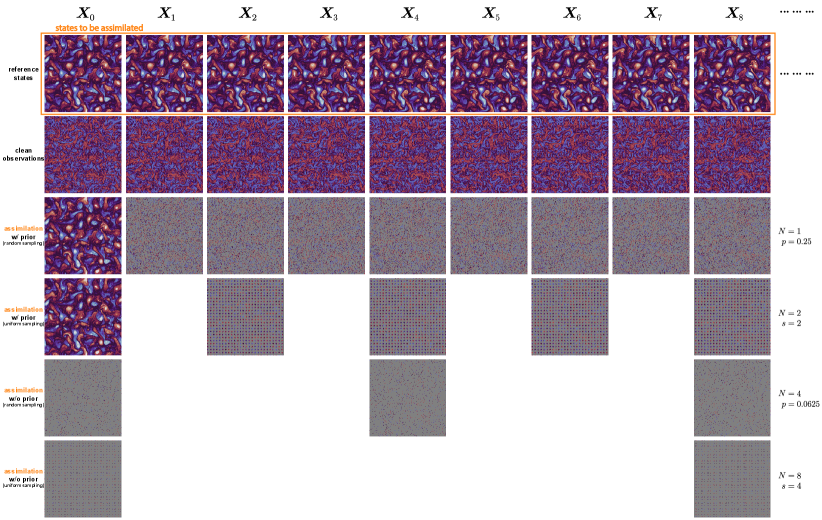
Since the evolution of the two-layer QG model does not depend on time, we assumes that the vorticity snapshots of shape within a fixed time range follow the same data distribution. Consequently, we divide each trajectory into 1,000 windows and retain only the first 32 snapshots from every 100 snapshots to avoid temporal correlations. Such a process transforms the dataset into windows of size . Figure 1 visualizes the generated data for a single time step.

4.2 network structures and training procedures
To ensure a fair comparison with the SDA baseline, we adopt the same network structure for the denoising network , which ultilizes a U-Net structure mixed with temporal convolutions and embeddings for diffusion time steps . The only difference between our network and the SDA baseline lies in the input channels because we require additional channels to concatenate the state variables with the clean observations to form the augmented states .
We use the first 8,000 windows for training and reserve the remaining 2,000 windows for valiation and testing. During training, a chunk of length 9 from each window of length 32 is selected randomly to create a mini-batch for the networks. All networks are trained with the Adam optimizer [27], employing a learning rate of and a weight decay of . To stabilize the training process, all inputs are normalized using the empirical mean and variance of the entire training dataset.
4.3 observations
To test our SOAD model and make comparisons with the baseline, we consider the following observational model
| (42) |
where denotes the time step index. consists of the two-layer vorticities at time step , and stands for the associated noisy observations.
We consider two different types of element-wise observations defined as
| (43) |
We refer to as the “easy” case since it is injective and monotonic, while is termed the “hard” case due to its highly nonlinear behavior. Apart from these straightforward choices, we also consider the vorticity-to-velocity mapping
| (44) |
to explore the potential of our model for real applications. Here, are the velocity components for the -th layer and denotes a multiplication with component-wise scalars so that the outputs approximately have zero means and unit deviations. Such a choice is inspired by the fact that velocity components are often directly observed rather than the related vorticity in the real world. To compute , (39) is solved for the streamfunctions in the spectral space, and then the velocity components are calculated by the streamfunctions. Note that we cannot conclude whether is easier or harder, as the operator is linear but the mapping rule is much more complex.
We test with subsampling matrices of two different types: random sampling from the grid with ratio , and uniform strided observation with stride , corresponding to a observational ratio222For spatial stride , the actual observational ratio is slightly above 1% since the snapshot size is not divisible by 10, but we omit this minor difference for simplicity.. To study assimilation performance using obserations with various time intervals, is set for every time steps. See Figure 2 for detailed illustrations.
4.4 assimilation
In the assimilation experiments, we fix our assimilation window to 9 time steps. This means we have observations subsampled from 9 consecutive steps, and our goal is to assimilate all the state variables within this time interval. We choose random ratios and strides for the subsampling with time intervals .
To make quantitative comparisons, we use the rooted mean-square error (RMSE)
| (45) |
to evaluate the assimilated state . Recall that consists of vorticities on two levels, and here we use for their normalized versions. is the reference solution, and stands for the spatial resolution. Since all the data have been normalized in advance, the RMSE results from different models and various assimilation settings are comparable. To decrease randomness, all the following experiments are run 5 times with different random seeds, and the averaged RMSEs are reported unless specified otherwise.
4.4.1 assimilation with prior
In practical applications, assimilation is usually performed sequentially once new observations become available, so we start with the classical assimilation settings that additionally provide the models with a background prior for the first step. We choose the background prior as an ideal Gaussian perturbation with a known covariance . Formally, the observational model for the first step is modified as
| (46) |
where is the background prior with noise variance . See Figure 2 (3rd and 4th rows) for visualization.
Our experiments start with the element-wise observations and . The averaged RMSEs over all the 9 time steps for the assimilated states are summarized in Figure 3.


Our SOAD model performs slightly worse as the time interval increases and the observational ratio or decreases, which aligns with our intuition that the assimilation task becomes more difficult with sparser observations. In the most challenging case, where the observations are available only every 8 time steps with a ratio of , the RMSEs are around 0.2 and 0.3 for the easy and hard observations, respectively. This indicates that our method is still able to extract the physical features from rare observations to some extent. In contrast, the SDA baseline shows a significant performance drop even when the observations are available everywhere for each time step. The inferior performance is likely due to the linearity assumption for the observation operator in the SDA formulations, which is unsuitable for highly nonlinear observations.
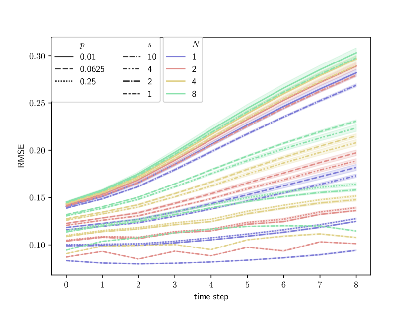
Additionally, the step-wise RMSEs for our SOAD model are exhibited in Figure 4. In both observation cases, The increments of RMSEs at observational ratios of 100% and 25% are mild, and no significant changes in RMSEs are observed when the easier is replaced with the harder . Moreover, relatively lower assimilation errors are obtained whenever observational data are available, supporting the idea that more observations enhance the assimilation process. By comparing results with the same observational ratios (), we may conclude that regular (uniform) observations are more beneficial for the assimilation process than irregular (random) ones.

To explore the potential of our SOAD model in real applications, we also test it with the vorticity-to-velocity mapping , and the results are shown in Figure 5. We do not include the performance of the SDA baseline since it diverges in all cases. Performances of the SDA baseline for are not included since it ends with divergence for all the cases. The averaged RMSEs in Figure 5(a) are lower than those in Figure 3(a) and Figure 3(c), which may be attributed to the linearity of the observational operator . The results indicate that our SOAD approach is capable of handling the vorticity-to-velocity mapping,a more practical observational model in real applications. Although SOAD shows faster increasing RMSEs with higher uncertainty for (Figure 5(b)) compared with and (Figure 4), the subsequent experiments may offer some evidences that the assimilation process is unlikely to diverge.


In practice, we cannot always expect the availability of the exact probability distribution for background prior. Background errors may result from many aspects, such as unresolved sub-scale features, temporal interpolations and physical parameterizations. Therefore, we investigate whether the discrepancy between our background prior model (46) and the real distribution affects the assimilation performance. We conduct experiments with the same settings as before but feed a background prior with unknown noise
| (47) |
into the model instead of . Here, is the forward propagation model of the QG equations, and stands for the snapshot at the previous time step. Comparisons between the step-wise RMSEs are displayed in Figure 6, where we fix and . Even with incorrect background prior assumptions, our SOAD model has the ability of self-correction with a few time steps of observations. Another interesting observation is that the RMSEs for the hard observation are lower than those for and . One possible explanation is that when the observational data is sufficient for the model to capture the dynamics, observations from a harder operator may provide more detailed information since is much more sensitive to the input.

4.4.2 assimilation without background prior
To explore the assimilation performance in the absence of any background prior, we remove the modification (46) and conduct the assimilation process solely from observational data. Even if starting with a background prior, any assimilation method will gradually forget the initial state information as more observations are assimilated. Therefore, the results shown in this section are likely to reveal the long-term behaviors of the assimilation methods.
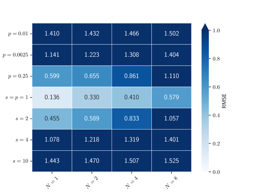
All assimilation results are recorded as heatmaps of RMSEs in Figure 7. In general, our SOAD model performs well for both the and the observations, with slightly higher accuracy for the latter. The observation appears to be the most challenging across all the testing observational operators.
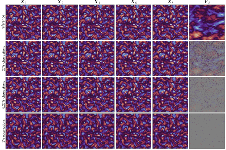
To visualize the assimilated states, we have plotted the assimilated vorticities with random observational ratios in Figure 8, Figure 9 and Figure 10 for , and , respectively. For clarity, we only include the vorticities and the associated observations for the first layer, as they contain more small-scale details. For the observation, our SOAD is capable of recovering most of the physical features until reaches , in which case the assimilated states still share much similarity with the ground truth. With the harder , the SOAD model fails to reconstruct the real system states when , consistent with the previous results shown in Figure 7(b). Surprisingly, the assimilated states with rare observations do not collapse and still follow certain dynamics, suggesting that the lack of observational data, rather than incapacity of learning the dynamics, leads to the failure. Finally, when the observation is the the vorticity-to-velocity mapping , the assimilated states are closer to the ground truth even when observations are available at only of the grids. We believe that the success may result from the linearity of . The results indicate that our SOAD approach is stable when handling highly nonlinear observations in the long term performs well on non-element-wise observations such as the vorticity-to-velocity mapping , which is a promising sign for real applications.


4.4.3 assimilation with multiple observations
In this subsection, we discuss another important features of our SOAD approach: the ability to handle observations from different modalities. Such a capability is crucial for real applications since the observations are usually collected from various sources like satellites, weather radars, and in-situ observations. Each source may provides different physical variables in different formats. We have tested our SOAD approach with various combinations of the three observations , and . Same as the previous subsection, we do not add any background prior for the first step in order to study the long-term behaviors. The results are displayed in Figure 11.


As the collection of observations expands, the uncertainties of the assimilation errors shrink, and the averaged RMSEs decrease as well due to the additional information inferred from the observations. This phenomenon implies that our SOAD approach also follows the intuitive principle that more observations are beneficial for the assimilation process. Figure 11(d) gathers the best performances for each observation collections when , and the overlapping areas are marked with the corresponding observation combinations.
5 Conclusion
In this study, we have proposed a noval data assimilation approach using the State-Observation Augmented Diffusion (SOAD) model, which does not rely on any traditional assimilation algorithms. Our SOAD model does not assume linearity for eith the physical or observational models, but it can still achieve the posterior probability under mild conditions, potentially offering an advantage over most traditional algorithms. The flexibility and applicability of our SOAD have been demonstrated in various testing settings on the two-layer quasi-geostrophic model, indicating its promise for future real-world applications.
One of the most significant features of our SOAD is the use of augmented dynamical models. The augmented model is essentially a linearized equivalent form associated with the original assimilation task, enabling us to focus on linear observational models even if the original problem are highly nonlinear. By using the score-based generative model as the backbone, our SOAD can learn the prior distribution of the physical states. Additionally, a deterministic estimation for the time-dependent marginal likelihood as well as a forward-diffusion corrector is proposed to help fuse the physical information embedded within the available observations with the state variables, which is crucial for the assimilation process.
Further improvements and extensions of our approach are also necessary. One possible direction is to analyze the convergence rates and conditions when considering training errors. The stability of the assimilation is one of the major concerns particularly in real-world applications. Moreover, the current SOAD approach has only been tested on the two-layer quasi-geostrophic model. Therefore, comprehensive tests on other idealized and real-world models is required to fully evaluate its effectiveness. Generalizing our SOAD approach to more complex tasks other than assimilation could also be a promising direction for future research.
Data availability
All the codes for data generation, network training and assimilation experiments are available at https://github.com/zylipku/SOAD.
References
- [1] Ryan Abernathey, rochanotes, Andrew Ross, Malte Jansen, Ziwei Li, Francis J. Poulin, Navid C. Constantinou, Anirban Sinha, Dhruv Balwada, SalahKouhen, Spencer Jones, Cesar B Rocha, Christopher L. Pitt Wolfe, Chuizheng Meng, Hugo van Kemenade, James Bourbeau, James Penn, Julius Busecke, Mike Bueti, and Tobias. pyqg/pyqg: v0.7.2, may 2022.
- [2] Maddalena Amendola, Rossella Arcucci, Laetitia Mottet, Cesar Quilodran Casas, Shiwei Fan, Christopher Pain, Paul Linden, and Yi-Ke Guo. Data assimilation in the latent space of a neural network. arXiv preprint arXiv:2012.12056, 2020.
- [3] Brian D.O. Anderson. Reverse-time diffusion equation models. Stochastic Processes and their Applications, 12(3):313–326, 1982.
- [4] Kaifeng Bi, Lingxi Xie, Hengheng Zhang, Xin Chen, Xiaotao Gu, and Qi Tian. Pangu-weather: A 3d high-resolution model for fast and accurate global weather forecast. arXiv preprint arXiv:2211.02556, 2022.
- [5] James Bradbury, Roy Frostig, Peter Hawkins, Matthew James Johnson, Chris Leary, Dougal Maclaurin, George Necula, Adam Paszke, Jake VanderPlas, Skye Wanderman-Milne, and Qiao Zhang. JAX: composable transformations of Python+NumPy programs, 2018.
- [6] Ashesh Chattopadhyay, Ebrahim Nabizadeh, Eviatar Bach, and Pedram Hassanzadeh. Deep learning-enhanced ensemble-based data assimilation for high-dimensional nonlinear dynamical systems. Journal of Computational Physics, 477:111918, 2023.
- [7] Kang Chen, Tao Han, Junchao Gong, Lei Bai, Fenghua Ling, Jing-Jia Luo, Xi Chen, Leiming Ma, Tianning Zhang, Rui Su, et al. Fengwu: Pushing the skillful global medium-range weather forecast beyond 10 days lead. arXiv preprint arXiv:2304.02948, 2023.
- [8] Shengchao Chen, Guodong Long, Jing Jiang, Dikai Liu, and Chengqi Zhang. Foundation models for weather and climate data understanding: A comprehensive survey. arXiv preprint arXiv:2312.03014, 2023.
- [9] Sibo Cheng, Jianhua Chen, Charitos Anastasiou, Panagiota Angeli, Omar K. Matar, Yi-Ke Guo, Christopher C. Pain, and Rossella Arcucci. Generalised latent assimilation in heterogeneous reduced spaces with machine learning surrogate models. J. Sci. Comput., 94(1), jan 2023.
- [10] Kyunghyun Cho, Bart Van Merriënboer, Dzmitry Bahdanau, and Yoshua Bengio. On the properties of neural machine translation: Encoder-decoder approaches. arXiv preprint arXiv:1409.1259, 2014.
- [11] Hyungjin Chung, Jeongsol Kim, Michael Thompson Mccann, Marc Louis Klasky, and Jong Chul Ye. Diffusion posterior sampling for general noisy inverse problems. In International Conference on Learning Representations, 2023.
- [12] A. M. Clayton, A. C. Lorenc, and D. M. Barker. Operational implementation of a hybrid ensemble/4d-var global data assimilation system at the met office. Quarterly Journal of the Royal Meteorological Society, 139(675):1445–1461, 2013.
- [13] Antonia Creswell, Tom White, Vincent Dumoulin, Kai Arulkumaran, Biswa Sengupta, and Anil A. Bharath. Generative adversarial networks: An overview. IEEE Signal Processing Magazine, 35(1):53–65, 2018.
- [14] Jacob Devlin, Ming-Wei Chang, Kenton Lee, and Kristina Toutanova. Bert: Pre-training of deep bidirectional transformers for language understanding. arXiv preprint arXiv:1810.04805, 2018.
- [15] Prafulla Dhariwal and Alexander Nichol. Diffusion models beat gans on image synthesis. Advances in neural information processing systems, 34:8780–8794, 2021.
- [16] Laurent Dinh, David Krueger, and Yoshua Bengio. Nice: Non-linear independent components estimation. arXiv preprint arXiv:1410.8516, 2014.
- [17] Carl Doersch. Tutorial on variational autoencoders. arXiv preprint arXiv:1606.05908, 2016.
- [18] A. J. Geer. Learning earth system models from observations: machine learning or data assimilation? Philosophical Transactions of the Royal Society A: Mathematical, Physical and Engineering Sciences, 379(2194):20200089, 2021.
- [19] Ian Goodfellow, Jean Pouget-Abadie, Mehdi Mirza, Bing Xu, David Warde-Farley, Sherjil Ozair, Aaron Courville, and Yoshua Bengio. Generative adversarial networks. Commun. ACM, 63(11):139–144, oct 2020.
- [20] Mohamad Abed El Rahman Hammoud, Naila Raboudi, Edriss S. Titi, Omar Knio, and Ibrahim Hoteit. Data assimilation in chaotic systems using deep reinforcement learning, 2024.
- [21] Jonathan Ho, Ajay Jain, and Pieter Abbeel. Denoising diffusion probabilistic models. arXiv preprint arxiv:2006.11239, 2020.
- [22] Jonathan Ho and Tim Salimans. Classifier-free diffusion guidance. arXiv preprint arXiv:2207.12598, 2022.
- [23] Sepp Hochreiter and Jürgen Schmidhuber. Long short-term memory. Neural Comput., 9(8):1735–1780, nov 1997.
- [24] Brian R Hunt, Eric J Kostelich, and Istvan Szunyogh. Efficient data assimilation for spatiotemporal chaos: A local ensemble transform kalman filter. Physica D: Nonlinear Phenomena, 230(1-2):112–126, 2007.
- [25] Andrew H Jazwinski. Stochastic processes and filtering theory. Courier Corporation, 2007.
- [26] Rudolph Emil Kalman. A new approach to linear filtering and prediction problems. 1960.
- [27] Diederik P. Kingma and Jimmy Ba. Adam: A method for stochastic optimization. In ICLR, 2015.
- [28] Diederik P Kingma and Max Welling. Auto-encoding variational bayes. arXiv preprint arXiv:1312.6114, 2013.
- [29] Alexander Kirillov, Eric Mintun, Nikhila Ravi, Hanzi Mao, Chloe Rolland, Laura Gustafson, Tete Xiao, Spencer Whitehead, Alexander C Berg, Wan-Yen Lo, et al. Segment anything. In Proceedings of the IEEE/CVF International Conference on Computer Vision, pages 4015–4026, 2023.
- [30] Ivan Kobyzev, Simon JD Prince, and Marcus A Brubaker. Normalizing flows: An introduction and review of current methods. IEEE transactions on pattern analysis and machine intelligence, 43(11):3964–3979, 2020.
- [31] Rahul G. Krishnan, Uri Shalit, and David Sontag. Deep kalman filters, 2015.
- [32] Remi Lam, Alvaro Sanchez-Gonzalez, Matthew Willson, Peter Wirnsberger, Meire Fortunato, Alexander Pritzel, Suman Ravuri, Timo Ewalds, Ferran Alet, Zach Eaton-Rosen, et al. Graphcast: Learning skillful medium-range global weather forecasting. arXiv preprint arXiv:2212.12794, 2022.
- [33] Zhuoyuan Li, Bin Dong, and Pingwen Zhang. Latent assimilation with implicit neural representations for unknown dynamics. Journal of Computational Physics, 506:112953, 2024.
- [34] Ze Liu, Yutong Lin, Yue Cao, Han Hu, Yixuan Wei, Zheng Zhang, Stephen Lin, and Baining Guo. Swin transformer: Hierarchical vision transformer using shifted windows. In Proceedings of the IEEE/CVF international conference on computer vision, pages 10012–10022, 2021.
- [35] Calvin Luo. Understanding diffusion models: A unified perspective. arXiv preprint arXiv:2208.11970, 2022.
- [36] Xiangming Meng and Yoshiyuki Kabashima. Diffusion model based posterior samplng for noisy linear inverse problems. arXiv preprint arXiv:2211.12343, 2022.
- [37] Jaideep Pathak, Shashank Subramanian, Peter Harrington, Sanjeev Raja, Ashesh Chattopadhyay, Morteza Mardani, Thorsten Kurth, David Hall, Zongyi Li, Kamyar Azizzadenesheli, et al. Fourcastnet: A global data-driven high-resolution weather model using adaptive fourier neural operators. arXiv preprint arXiv:2202.11214, 2022.
- [38] Suraj Pawar and Omer San. Equation-free surrogate modeling of geophysical flows at the intersection of machine learning and data assimilation. Journal of Advances in Modeling Earth Systems, 14(11):e2022MS003170, 2022.
- [39] S. G. Penny, T. A. Smith, T.-C. Chen, J. A. Platt, H.-Y. Lin, M. Goodliff, and H. D. I. Abarbanel. Integrating recurrent neural networks with data assimilation for scalable data-driven state estimation. Journal of Advances in Modeling Earth Systems, 14(3):e2021MS002843, 2022.
- [40] Mathis Peyron, Anthony Fillion, Selime Gürol, Victor Marchais, Serge Gratton, Pierre Boudier, and Gael Goret. Latent space data assimilation by using deep learning. Quarterly Journal of the Royal Meteorological Society, 147(740):3759–3777, 2021.
- [41] Danilo Rezende and Shakir Mohamed. Variational inference with normalizing flows. In International conference on machine learning, pages 1530–1538. PMLR, 2015.
- [42] Robin Rombach, Andreas Blattmann, Dominik Lorenz, Patrick Esser, and Björn Ommer. High-resolution image synthesis with latent diffusion models. In Proceedings of the IEEE/CVF conference on computer vision and pattern recognition, pages 10684–10695, 2022.
- [43] François Rozet and Gilles Louppe. Score-based data assimilation. In Thirty-seventh Conference on Neural Information Processing Systems, 2023.
- [44] François Rozet and Gilles Louppe. Score-based data assimilation for a two-layer quasi-geostrophic model. 2023.
- [45] M. G. Schultz, C. Betancourt, B. Gong, F. Kleinert, M. Langguth, L. H. Leufen, A. Mozaffari, and S. Stadtler. Can deep learning beat numerical weather prediction? Philosophical Transactions of the Royal Society A: Mathematical, Physical and Engineering Sciences, 379(2194):20200097, 2021.
- [46] Xingjian Shi, Zhourong Chen, Hao Wang, Dit-Yan Yeung, Wai-Kin Wong, and Wang-chun Woo. Convolutional lstm network: A machine learning approach for precipitation nowcasting. Advances in neural information processing systems, 28, 2015.
- [47] Uriel Singer, Adam Polyak, Thomas Hayes, Xi Yin, Jie An, Songyang Zhang, Qiyuan Hu, Harry Yang, Oron Ashual, Oran Gafni, et al. Make-a-video: Text-to-video generation without text-video data. arXiv preprint arXiv:2209.14792, 2022.
- [48] Casper Kaae Sønderby, Tapani Raiko, Lars Maaløe, Søren Kaae Sønderby, and Ole Winther. Ladder variational autoencoders. Advances in neural information processing systems, 29, 2016.
- [49] Jiaming Song, Chenlin Meng, and Stefano Ermon. Denoising diffusion implicit models. arXiv preprint arXiv:2010.02502, 2020.
- [50] Yang Song, Jascha Sohl-Dickstein, Diederik P Kingma, Abhishek Kumar, Stefano Ermon, and Ben Poole. Score-based generative modeling through stochastic differential equations. In International Conference on Learning Representations, 2021.
- [51] Simo Särkkä and Arno Solin. Applied Stochastic Differential Equations. Institute of Mathematical Statistics Textbooks. Cambridge University Press, 2019.
- [52] Hugo Touvron, Thibaut Lavril, Gautier Izacard, Xavier Martinet, Marie-Anne Lachaux, Timothée Lacroix, Baptiste Rozière, Naman Goyal, Eric Hambro, Faisal Azhar, et al. Llama: Open and efficient foundation language models. arXiv preprint arXiv:2302.13971, 2023.
- [53] Ashish Vaswani, Noam Shazeer, Niki Parmar, Jakob Uszkoreit, Llion Jones, Aidan N Gomez, Łukasz Kaiser, and Illia Polosukhin. Attention is all you need. Advances in neural information processing systems, 30, 2017.
- [54] Pascal Vincent. A connection between score matching and denoising autoencoders. Neural computation, 23(7):1661–1674, 2011.
- [55] Athanasios Voulodimos, Nikolaos Doulamis, Anastasios Doulamis, and Eftychios Protopapadakis. Deep learning for computer vision: A brief review. Computational Intelligence and Neuroscience, 2018(1):7068349, 2018.
- [56] Ling Yang, Zhilong Zhang, Yang Song, Shenda Hong, Runsheng Xu, Yue Zhao, Wentao Zhang, Bin Cui, and Ming-Hsuan Yang. Diffusion models: A comprehensive survey of methods and applications. ACM Computing Surveys, 56(4):1–39, 2023.
- [57] Yiyuan Yang, Ming Jin, Haomin Wen, Chaoli Zhang, Yuxuan Liang, Lintao Ma, Yi Wang, Chenghao Liu, Bin Yang, Zenglin Xu, et al. A survey on diffusion models for time series and spatio-temporal data. arXiv preprint arXiv:2404.18886, 2024.
- [58] Qinsheng Zhang and Yongxin Chen. Fast sampling of diffusion models with exponential integrator. arXiv preprint arXiv:2204.13902, 2022.
- [59] Wayne Xin Zhao, Kun Zhou, Junyi Li, Tianyi Tang, Xiaolei Wang, Yupeng Hou, Yingqian Min, Beichen Zhang, Junjie Zhang, Zican Dong, et al. A survey of large language models. arXiv preprint arXiv:2303.18223, 2023.
- [60] Shujun Zhu, Bin Wang, Lin Zhang, Juanjuan Liu, Yongzhu Liu, Jiandong Gong, Shiming Xu, Yong Wang, Wenyu Huang, Li Liu, Yujun He, Xiangjun Wu, Bin Zhao, and Fajing Chen. A 4denvar-based ensemble four-dimensional variational (en4dvar) hybrid data assimilation system for global nwp: System description and primary tests. Journal of Advances in Modeling Earth Systems, 14(8):e2022MS003023, 2022. e2022MS003023 2022MS003023.
Appendix A Configurations of the two-layer quasi-geostrophic model
We list the parameters (as defaults in pyqg-jax333https://pyqg-jax.readthedocs.io/en/latest/reference.models.qg_model.html) we used to generate the QG test dataset.
-
•
Domain size: ;
-
•
Linear drag in lower layer: ;
-
•
Amplitude of the spectral spherical filter with parameter to obtain the small-scale dissipation;
-
•
Gravity: ;
-
•
Gradient of coriolis parameter: ;
-
•
Deformation radius: ;
-
•
Layer thickness: , ;
-
•
Upper/Lower layer flow: , .
Readers may refer to pyqg444https://pyqg.readthedocs.io/en/latest/equations/notation_twolayer_model.html for the detailed numerical stepper.