State-dependent driving: A route to non-equilibrium stationary states
Abstract
We study three different experiments that involve dry friction and periodic driving, and which employ both single and many-particle systems. These experimental set-ups, besides providing a playground for investigation of frictional effects, are relevant in broad areas of science and engineering. Across all these experiments, we monitor the dynamics of objects placed on a substrate that is being moved in a horizontal manner. The driving couples to the degrees of freedom of the substrate, and this coupling in turn influences the motion of the objects. Our experimental findings suggest emergence of stationary-states with non-trivial features. We invoke a minimalistic phenomenological model to explain our experimental findings. Within our model, we treat the injection of energy into the system to be dependent on its dynamical state, whereby energy injection is allowed only when the system is in its suitable-friction state. Our phenomenological model is built on the fact that such a state-dependent driving results in a force that repeatedly toggles the frictional states in time, and serves to explain our experimental findings.
1 Introduction
A common parlor trick to demonstrate inertia is to place a coin on a post card, and then quickly pull the card. If the pull is quick enough, the coin remains almost in its place while the card gets pulled out. While the trick and its many variations (pulling a book out of a stack of books, or, the game Jenga) are themselves very instructive, they nevertheless leave a few pertinent questions related to the stationary-state dynamics unanswered. The coin is attached to the card by forces of friction. Common wisdom tells us that if the acceleration of the card is larger than a critical value, the coin will begin to slip with respect to the card. However, as soon as the coin starts to slip, a crack opens up on the interface [1, 2], and this results in weakening of the frictional coupling between the card and the coin. Since there is dissipation, the coin loses momentum and eventually heals the crack, and the frictional coupling regains its strength. The whole process of weakening and strengthening of the frictional coupling undergoes repeated cycles in time. In such a scenario, does the coin eventually move with uniform velocity or does it accelerate? In this paper, we will show that the qualitative aspects of this particularly simple experiment and some variants of it can be explained in terms of a phenomenological model in which the rate of energy injection into a system depends on its dynamical state.
1.1 Degrees of freedom and internal states of a system
In a more general setting, the aforementioned scenario would be an example of an interacting system evolving in presence of drive and dissipation. In our studied systems, input of energy through the external drive at the level of the substrate (e.g., the card) affects the evolution of the frictional states of the objects (e.g., the coin) placed on the substrate and may cause in time random transitions between the different frictional states. These transitions in turn would act back on the time evolution of the objects, resulting in an intricate (and intriguing, in many-body complex systems) interplay between the dynamics of the objects and that of the frictional states [3, 4]. In the context of the coin and the plate, the qualitatively different frictional states are that of slipping (low-friction state) and sticking (high-friction state). If the coin is replaced by a sphere, then the frictional states may be identified with rolling (low-friction state) and sliding (high-friction state) motion.
It is evidently of interest to ask: what is the long-time behavior of the aforementioned class of systems? Does the system achieve a stationary state with a time-independent distribution of the degrees of freedom of the objects? We may in general anticipate that a balance between drive and dissipation does in fact lead the system to a stationary state. Presence of an external drive precludes the possibility for the stationary state to be an equilibrium one. Consequently, any stationary state the system relaxes to at long times would be a generic nonequilibrium stationary state (NESS) [5]. In this work, we highlight the subtleties that come into play in the dynamics, by presenting three experiments - (i) a single coin on a platform oscillating along one axis and (ii) a single sphere and (iii) a collection of spheres placed on an orbiting platform [6]. The first experiment is one dimensional in nature, and from its detailed study, we establish that at a phenomenological level, the coupling between the plate and the coin can be modeled by a viscous force-like velocity dependent term. In the second experiment, the center-of-mass of the sphere covers a two-dimensional space, and it does so under the influence of two orthogonal forces. From this experiment, we establish that the stochasticity in the trajectory of the sphere comes from the randomness in the amplitudes of the two orthogonal forces. In the third experiment, we introduce interactions between the particles, and establish that the resulting velocity distribution attains a unique velocity distribution with the tail, which is exponential in nature, gaining weight with increasing density of spheres. This observation is surprising, since collision-induced cooling is at the heart of many observable NESS states in granular systems.
Following the experimental results, we present a minimalistic one-particle theoretical model that captures the essence of the experimental findings, and provides us with a framework to understand such scenarios. Within our model, we treat the injection of energy to the system to be dependent on its dynamical state, whereby energy injection is allowed only when the system is in a suitable-friction state of the system. The idea of state-dependent driving is rooted in various biological systems, where the functionality of a state is maintained by an organism by constantly regulating the activity of its various internal processes. In the context of active systems, this would translate to the idea of prescribing a local density-dependent mobility to the particles. It is known that such quorum-sensing interactions can give rise to motility-induced phase transitions [7]. Another example is that of enzymes locally enhancing diffusion by self-regulating the phoretic [8] and hydrodynamic forces generated by themselves. This can lead to such functional behavior as antichemotaxis [9].
1.2 Dry friction models and their limitations
The experiments and numerics presented in this paper are considered for frictional systems. At a first glance, the experimental scenarios considered here might appear commonplace and well studied. It is thus important that we discuss the conventional method of treating apparently similar problems using the well-established framework of friction and point out the differences between the ones that are exhaustively discussed in the literature from the ones studied here.
The problem with dry friction:
A solid that is frictionally coupled to a substrate is put to motion when the force applied to the body exceeds , where is the normal force exerted by the solid on the substrate and is the coefficient of friction. When the relative velocity between the substrate and the body is zero, then , the coefficient of static friction, and , where is the force of friction. However, when the object is in motion, then , the coefficient of kinetic friction, and . Here is a positive real number that characterizes the transition from a stuck to a moving phase, and is also a positive real number that characterizes the friction forces when the object is slipping with respect to the substrate. The above description is the Coulomb description of dry friction. For other phenomenological models of dry friction, see Ref. [10]. In general, the coefficients of friction are defined for a pair of materials, and . Thus, forms an admissible set , i.e., . Unlike viscous friction, where as , there exists a velocity gap in dry friction, i.e., the velocity becomes zero if the magnitude of the applied force becomes smaller than a threshold value [11]. Dry friction breaks the time-reversible symmetry associated with the dynamics of bodies. This loss of symmetry is sometimes reflected in the non-linear (often chaotic) dynamics exhibited by these systems [12, 13]. The presence of an admissible set of friction values and the velocity gap makes the problem of dry friction not amenable to an analysis within the framework of deterministic dynamics.
Modeling Friction as a mechanical instability:
Friction is considered to be a nonlinear phenomenon [14], and models like the Prandtl-Tomlinson associate this nonlinearity with mechanical instabilities (for an historical account, see Ref. [15, 16]). Within the framework of these models, the overall response of the mechanical system is understood in terms of the ratio of two potentials: one associated with the substrate - body interaction and the other associated with elastic coupling between the body and an external anchor point [17, 18]. This anchor point can either remain stationary or have a well-defined trajectory. If the ratio of these two potentials is less than one, the overall motion of the body is smooth. On the other hand, when this ratio is large, the sliding motion becomes jagged (slip-stick motion), and the system continuously exhibits a series of elastic instabillity transitions (see chapter 10 of Ref. [18]). Thus, Prandtl-Tomlinson is essentially a two-body model which in itself or whose close variants like the ones that incorporate stress-augmented thermal activation process [19] has been successfully used to understand a wide range of frictional problems encountered in experimental studies using a variety of friction force microscopes (FFM) [16, 15, 20]. The dynamics of the model that comprises a single particle being dragged with velocity on a one-dimensional substrate considered to be a sinusoidal potential is described by the equation of motion
| (1) |
where represents Gaussian, white noise satisfying and is the temperature. In the above equation, is the damping coefficient, while the force is obtained from the potential . Here, and are respectively the amplitude and the periodicity of the sinusoidal potential, while represents the strength of the harmonic coupling between the particle and the substrate. Friction associated with extended objects is treated within the framework of Frenkel-Kontorova (FK) like models [21]. Here, the elastic energy associated with the coupling between the body and the anchor point is replaced by the energy associated with the deformation of the body itself. As a result, the response of soft objects in presence of frictional force is very different from that of the more rigid ones - a phenomenon that is known as the Aubry transition [22]. Rigid objects tend to move smoothly, while soft objects exhibit slip-stick motion.
Almost all experimental realizations in friction are classified into two types, one where the force is directly applied to the object, e.g., an atomic force microscope tip being dragged over a substrate or where the body is held with a spring to a point in space and the substrate moves below it [23, 24, 25, 26]. In either case, the two competing energy scales can be easily identified and hence, these situations are amenable to detailed analysis. However, there may be situations, e.g. coin on a horizontally vibrating plate [27], where identifying two separate energies, one of which is due to the application of a force on the system of interest and the other due to its motion against a frictionally-coupled substrate, may not be possible. This happens when the processes by which energy is injected and dissipated are not separated in space and time. This is precisely the dynamical scenario that we address in this work.
Stochastic aspects of Friction:
Though the force of friction is an easily measured quantity, its value is highly sensitive to experimental conditions. Often, measured friction forces vary from one experiment to another and also these are known to strongly age with time [28, 29]. For dry friction, the local structure of the interlocking interfaces plays a key role. Since the area of this interlocking region is small, each patch of the interface corresponds to different values of friction. This lack of self-averaging necessitates the use of a stochastic dynamics to study the problem. In doing so, one may invoke stochasticity in the configuration space through the modeling of making and breaking of contacts [30, 31]. Alternatively, one may invoke stochasticity in the energy space whereby energy injection and dissipation are modeled as stochastic processes. In this paper, in contrast to earlier work, we follow the second approach and propose a model in which the energy transfer between a moving substrate and a body is treated as a stochastic variable whose value depends on the ‘state’ of the system. Here, we use the term ‘state’ in the same sense as described in the leading paragraph of Sec. 1.1. One may recall that phenomenological models of friction like the ‘rate-state model’ [32, 33, 34, 35] also invoke the concept of states in a different sense, without however explicitly identifying the states. However, many recent works have attempted to do so by treating friction as localized electro-plastic response of the contact zone [36].
2 Results
2.1 A coin on an oscillating plate
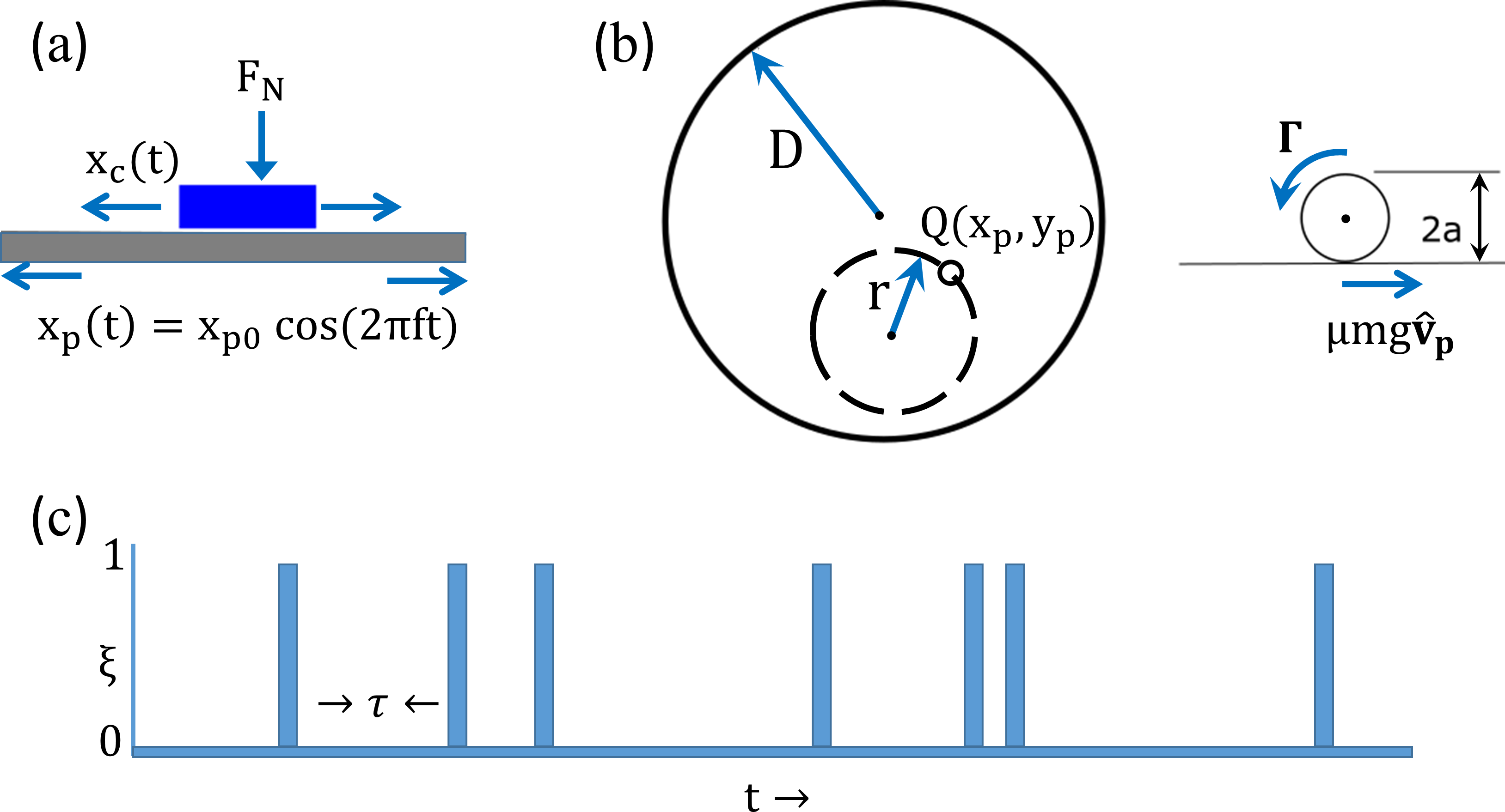
A coin is placed on a plate that is being vibrated in the direction, see Fig. 1(a). The motion of both the coin and the plate is measured simultaneously. The plate moves sinusoidally, , where is the position of a point on the plate, is the amplitude of vibration, and is the driving frequency.
2.1.1 Experimental results
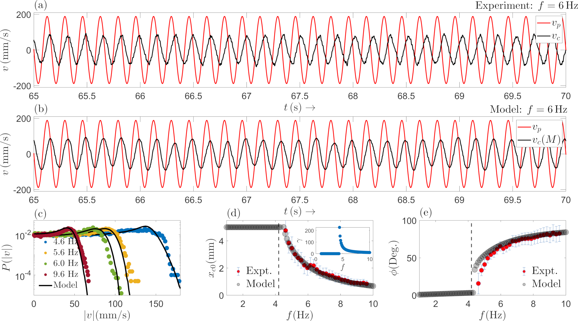
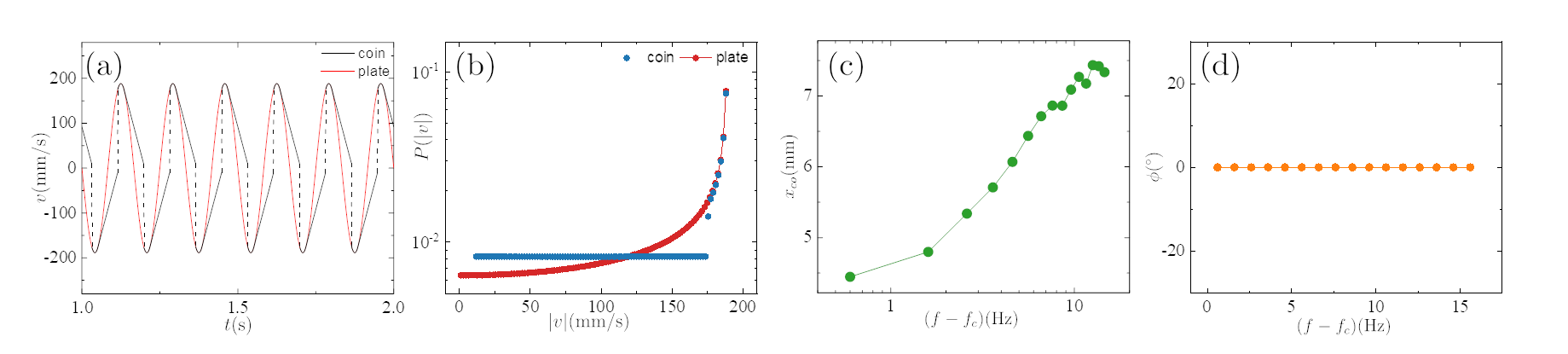
For small values of , the coin remains stuck to the plate, while for larger values of , it begins to slip with respect to the plate. Typical time traces of the velocity of the center of mass of the coin and a point fixed on the plate for Hz are shown in Fig. 2(a). In the phase in which the coin slips with respect to the plate, its center of mass drifts slowly in time. However, for small time intervals, its response , namely, the location of its center of mass, is approximately sinusoidal, and has the same frequency of variation as that of the plate. The probability distribution of , the magnitude of the velocity of the center of mass of the coin, is plotted in Fig. 2(c); the distribution is obtained by sampling the trajectories in the long-time limit over a time window. The variation of the time-averaged amplitude of displacement of the coin and its phase difference with respect to the plate in the long-time limit is plotted in Fig. 2, panels (d) and (e), respectively, as a function of the driving frequency.
Our main experimental observations may be summarized as follows:
-
1.
At long times, the velocity as well as the displacement of the coin is approximately sinusoidal in time (Fig. 2(a)).
-
2.
The velocity distribution of the coin has a tail that is exponential (Fig. 2(c)).
-
3.
The time-averaged amplitude of the displacement of the coin decreases with the drive frequency (Fig. 2(d)).
-
4.
The phase difference saturates to a large value with increase in the drive frequency (Fig. 2(e)). This is in contrast to what is seen in the case of a damped, driven harmonic oscillator with a real damping constant, which in turn precludes use of noisy harmonic oscillator to model our experimental scenario. The case of a complex damping constant is discussed in the appendix.
2.1.2 Discussion
The most evident way to describe the system would be to use the Coulomb friction model [18]. If the driving frequency is such that the amplitude of the sinusoidal forcing exerted by the plate is larger than the maximum static friction force, i.e., , with being the coefficient of static friction between the coin and the plate and the mass of the coin, the coin will undergo both stick and slip motion periodically. In the stuck state, i.e., when , trajectory of the coin will follow the sinusoidal nature of the trajectory of the plate. However, as soon as the driving force exceeds , the coin will start to slip with respect to the plate and it will then move under a constant acceleration due to the force of kinetic friction . Here, is the coefficient of kinetic friction between the coin and the plate. Hence, the velocity of the coin will be partly sinusoidal and partly linear in a single period. This model gives rise to a deterministic velocity profile. This is in stark contrast to the noisy sinusoidal nature of the velocity observed in the experiments. In addition, the velocity distribution, the amplitude and the phase response of the coin as obtained from the Coulomb friction model of friction is very different from what is observed in the experiments. We have provided the details in the appendix.
2.1.3 Model
The response of the system for and is qualitatively different. For , the coin and the plate behave as a single rigid object, i.e., , which is unlike the situation for . The description below is limited to the latter case only.
Experiments suggest that the coin never gets stuck to the plate at the smallest time scale over which the motion of the coin and the plate is measured, i.e., . Hence, to explain the experimental observations, we propose that the coin has access to (i) a ‘high-friction’ state (which in a limiting case becomes the stuck state) and (ii) a ‘low-friction’ state (or a slip state). Without the presence of ‘high-friction’ state, the coin would never experience the external driving applied to the plate and hence, the response of the coin would never reflect the waveform of the drive. However, over a large parameter regime, we find that the amplitude of the coin is smaller than that of the plate. Thus, it is reasonable to assume that the ‘high-friction’ state survives over a timescale that is smaller than the smallest time scale of measurement, and that during this time scale, , a fraction of the momentum of the plate gets transferred to the coin. Here, it becomes necessary to differentiate between a ‘stuck’ state (observed for ) and a ‘high-friction’ state. In contrast to a ‘high-friction’ state, in a ‘stuck’ state, the entire momentum and hence, the entire force would be transferred from the plate to the coin. We assume the transitions between the high-friction and the low-friction state to occur randomly in time. We thus propose a stochastic variant of the Coulomb friction model for the motion of the coin on the vibrated plate which captures the essential qualitative features of its dynamics observed in the experiments described above.
To be consistent with the experiment, we choose to describe the motion of the center of mass of the coin in an inertial frame, i.e., in the laboratory frame. With respect to such a frame, the plate on which the coin is placed is being vibrated sinusoidally in time, so that its velocity at time reads . When the coin is in the ‘high-friction’ state, the equation of motion of its center of mass is the usual Newton’s equation of motion:
| (2) |
where is the velocity of the coin, while is the force experienced by the coin due to transfer of momentum from the plate to the coin. Here, the quantity is the mass of the plate and as defined earlier is the timescale over which the ‘high-friction’ state survives and during which the momentum of the vibrating plate is transferred to the coin. On the other hand, when the coin is in the ‘low-friction’ (slip) state, it is detached from the plate, and consequently, it moves in presence of an effective damping force that dissipates in time the initial momentum of the coin at the instant of detachment from the plate. Hence, in the ‘low-friction’ state, the equation of motion of center of mass is given by , where is a phenomenological dissipation constant. The coin toggles randomly in time between the ‘high-friction’ and the ‘low-friction’ state. Introducing a random variable taking on values 1 or 0 corresponding to the ‘high-friction’ and the ‘low-friction’ state, respectively, one may on the basis of the foregoing write down the equation of motion of the center of mass as a stochastic differential equation, a Langevin-like equation, of the form
| (3) |
Equation (9) has to be supplemented by another equation describing the time evolution of the instantaneous , namely, . While derivation of an exact form of the latter would invariably involve a detailed modeling of the dynamics of the contact region via which the friction force is transmitted, we here offer a phenomenological description for the evolution of in terms of a stochastic Markov process, namely, between times and , the variable is updated to read with probability , while with the complementary probability . Here, is a dynamical parameter. It then follows that the random time between two successive occurrences of the value unity for is distributed as an exponential: , and that the average is given by . As a function of time, appears as a set of impulses distributed randomly in time, as shown in Fig. 1(c). For a given drive, the parameter is a phenomenological parameter. To fit our experimental data we require . This suggests strain rate induced weakening of the contact zone which could possibly arise from the reduction of contact area with increasing strain rate [37]. A reduction in results in re-scaling of the relaxation time , which thereby influences the momentum transfer process via . For the coin to slip, the contact zone must reach a critical size [38]. Further, given describes the dynamics at the contact it also likely to influence the time scale associated with the growth of the slip region of the contact zone. We thus assume to be a function of . This forms the rationale for assuming a linear dependence between and which is used to fit the data. The specific forms of and as a function of are given in the appendix.
It is interesting and pertinent that we draw a parallel between Eq. (9) and the usual form of the Langevin equation that one encounters in describing say the paradigmatic Brownian motion. Besides the nature of the stochastic noise, which in the latter is a Gaussian, white noise and in Eq. (9) is a dichotomous noise, one very important difference is the following. In the case of the Brownian motion, the strength of the noise term is a constant that does not depend on the value of the dynamical variable in question (more precisely, the constant is by virtue of the fluctuation-dissipation theorem related to the equilibrium temperature of the ambient medium). By contrast, in Eq. (9), the strength of the noise term is explicitly dependent on the value of the dynamical variable being studied. Another point worth mentioning is that the noise in the case of Brownian motion is considered stationary, while in our case, the noise is non-stationary.
Another interesting parallel that one may draw is between the dynamics (9) and the dynamics of a driven, damped harmonic oscillator evolving in presence of noise. In such an approach, one may consider the noise to be multiplicative, in the sense that it appears as a coefficient of the damping term in the dynamics, i.e., . The problem with this approach is that even when the coin is slipping, there will be the unphysical dynamics of momentum transfer between the coin and the plate. In contrast, the model presented here is nevertheless founded on physical reasoning, as presented in the paragraph preceding Eq. (9).
Note that in the dynamics described by Eq. (9), the force
experienced by the coin is being continually reset in time between the
pure sinusoidal drive and the entirely dissipative form as the random
variable toggles in time between its two-possible values.
Equation (9) may be considered representative of a class of stochastic dynamical systems in which the force resets stochastically in time between a set of possible values, the two-state process considered here being the simplest one may conceive.
The dynamics described by Eq. (9) involves two time scales
, setting the average time between two impulses, and
. We work in the regime in which . Consequently,
in the long-time limit, we expect the velocity to vary sinusoidally
in time with occasional jump in values as an effect of toggling acting
on a time scale that is faster compared to the sinusoidal variation.
As far as the parameter is concerned, its magnitude would set
the cut-off scale of the velocity in the slip state.
Figure 2, panels (b)-(e) compare the results obtained from numerical simulation of the dynamics (9) with the experimental findings. In panel (b), we see that consistent with our expectations mentioned above, the velocity does represent an almost sinusoidal variation in time and correspondingly, the velocity distribution in (c) exhibits a peak at a value around the amplitude value of the sinusoidal variation in (b). The toggling phenomenon manifests itself as deviations from a pure sinusoidal variation in (b) and contributes to a width around the peak in the distribution in (c). It is remarkable that our phenomenological model (9) is able to reproduce in a rather striking manner the experimental features of the coin dynamics in (a) and the velocity distribution in (c). Moreover, the distribution has a tail that is exponential, as seen in panel (c). In simulations, this is a result of dissipation set by in the dynamics (9). Moreover, the amplitude and the phase response as obtained from the simulations are in good agreement with the experimental data (see Fig. 2 (d) and (e)). As for the coin-trick problem that was proposed in the introduction, we expect the coin to move with a constant velocity. The magnitude of the velocity would depend on the coefficient of friction and the acceleration of the card being pulled out.
2.2 A sphere on an orbital shaker
In the above experiment, the stochasticity in the forcing term arises
from the toggling between the ‘high-friction’ and the ‘low-friction’ state of the coin. In the
second experiment that we describe now, we place a stainless steel ball (a sphere of mass , radius , and moment of inertia ) on a plate connected
to an orbital shaker. The schematic setup of the experimental setup is shown in Fig. 1(b).
Here, the system can toggle between the rolling (without slipping) and the sliding state. With an orbital shaker, the plate moves in an orientation-preserving manner such that each point on the plate moves on a circle of the same radius : a given point on the plate moves as , , where is the center of the circle about which the chosen point moves. Each point on the plate has a center associated with it. The motion of the sphere comes from the force that is exerted at the point of contact between the sphere and the moving plate. This frictional force affecting the velocity of the center of mass of the ball as , with the coefficient of friction, the acceleration due to gravity, and being the velocity of a point on the plate, exerts a torque about an axis parallel to the platform and passing through the center of mass of the sphere, i.e.,
| (4) |
where is the angular velocity of the sphere.
An isolated sphere on the plate performs a swirling motion
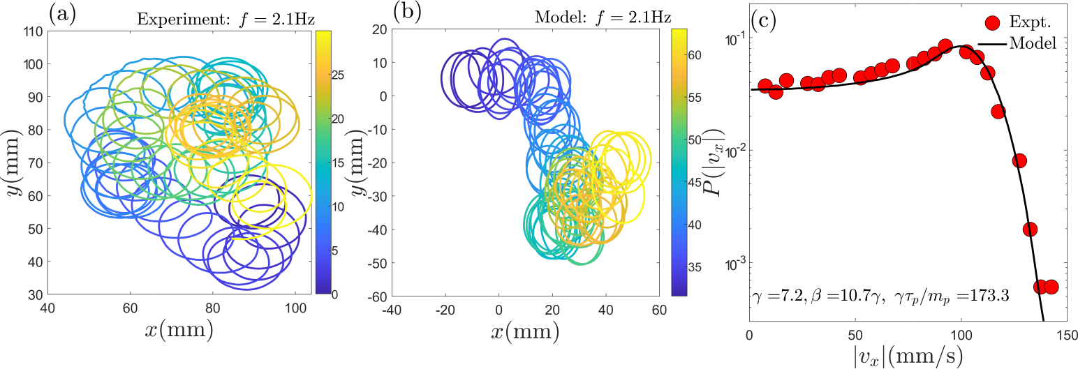
[39, 40, 6]. An example of such a motion for in the reference frame of the moving plate is shown in Fig. 3(a). In experiments, the long-time
trajectory of both the position and the velocity of the sphere is not
deterministic.
2.2.1 Experimental results
Effectively, this is a two-dimensional
version of the previous problem, wherein the particle-substrate
interaction generates the randomness in the motion. Individually, both the - and the
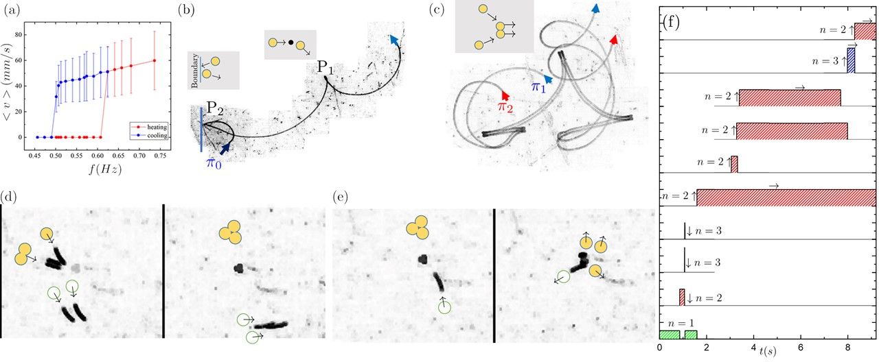
-components of the motion are approximately sinusoidal in nature. The abrupt alteration in the trajectory marked as in Fig. 4 (b) is an example of such scattering. Occasional collisions
with the boundary leads to additional randomness in the trajectories. An instance of this kind of scattering is shown as in Fig. 4 (b). These scattering events introduce a random phase difference between the two components which
results in the randomization of the trajectories.
The probability
distribution of the magnitude of the -component of the velocity, ,
of a rolling sphere for representative value of is plotted in
Fig. 3(c). A similar distribution is seen for also. In
the tails, the velocity distribution varies as , with . This is very
different from the well-known Maxwell distribution, in which case .
2.2.2 Model
Similar to previous experiment, we postulate that the noise in the trajectory arises from occasional slipping of the ball with respect to the plate. These partial slips have a concomitant toggling between the sliding and the rolling state of the system, and hence, similar to the previous example, the resulting noise can also be considered dichotomous. Thus, the Langevin-like equation of motion of the velocity of the center of mass of the ball has the form
| (5) |
with . Here, and correspond to sliding and rolling states respectively. It is to be noted that contrary to the coin on the plate problem, here momentum transfer from the plate to the sphere happens in the rolling (‘low-friction’) state. This is due to the fact in a pure rolling motion (without slipping), the contact point of the sphere is temporarily at rest with respect to the plate. On the other hand, in the sliding state which in this case is a relatively ‘high-friction’ state, the sphere moves in the presence of the damping force.
However, when there are more than one particle in the system, the inter-particle collisions also contribute to the over all noise in the trajectories. In the following subsection, we consider the case of many spheres on an orbital shaker.
2.3 Collection of spheres on an orbital shaker
In the third experiment, we put number of balls on the same setup. Care has been taken to ensure that the driven plate is kept as much horizontal as possible which can be seen from the inset in Fig. 5 (b). It shows the averaged intensity of a stack of 600 images taken at an interval of 1 s. The homogeneous distribution of particle density clearly shows that particles are mostly concentrated at the center of the plate. This also indicates that particle-wall collisions occur rarely as compared to inter particle collisions (wall is indicated by the dotted circular red line).
2.3.1 Experimental Results
The trajectories shown in Fig. 4 (b) and (c) are obtained by averaging a sequence of images, each taken with a time interval of ms. The micrographs in Fig. 4 (c) to (d) highlight the influence exerted by one particle on the other. When two spheres collide tangentially, two events can occur - (i) the spheres alter their direction and continue swirling, or, (ii) they form a bound dyad-like pair; This pair moves together mostly in a reciprocating manner, rolling back and forth in the direction that is perpendicular to the line joining the centers of the two balls. In the direction that is along the line joining the two centers, the pair does a sliding motion. Figure 4(c) shows two trajectories and that correspond to a collision and formation of a transiently stable dyad structure. In its dyad form, the two trajectories move parallel to each other. This structure is short lived and often spontaneously break apart. When it does so, the trajectories and depart from each other. The destabilization of the dyads can be brought about either by a particle-substrate or a particle-particle scattering event. In the case of the trajectory shown in Fig. 4(c), it is the particle-substrate scattering that destabilizes the dyad.
Occasionally, a third ball bumps into the two-particle pair. This can either destabilize the dyad or can form a compact three-particle triad. For spheres in contact, rolling in the same direction causes shearing of the contact region [3]. Thus, a triad cannot roll and, hence, it either becomes static or does small sliding motion. Figure 4(d) shows a sequence of micrographs that captures the event corresponding to the formation of the triad. These micrographs are obtained by using exposure time of ms. This long exposure produces a motion-induced dilation effect of the objects. Thus, moving objects in these micrographs will appear extended, and its shape tells us about the nature of motion, e.g., a roller’s motion will appear as a curved line, and dyads will appear as parallel straight lines. For static objects, motion-induced elongation is absent, and the objects appear as dots. The leftmost frame shows a dyad and a nearby rolling isolated sphere. The other two particles in the frame are present to provide a reference.
After collision, the three spheres form a static triad. Absence of substantial motion for this triad can be inferred from the lack of motion- induced dilation (see the second frame of the micrograph in Fig. 4 (d) and first frame in Fig. 4 (e)). For any higher-order structure involving more than 3 spheres that can form, the only available mode of movement is sliding. So the transitions in these structures are limited to stuck to sliding states. For the values of reported in this paper, the clusters (dyads, triads and higher order structures) are only transiently stable. Structures involving more than 3 particles are destabilized by particle collisions. An instance of this destabilization can be seen in Fig. 4(e). Figure 4(f) shows the corresponding sequence of formation and dissolution of particle clusters for a system of 11 particles that is being driven. The system begins with no clustering, i.e., and then quickly shows clustering. We find that dyads are the most frequently formed clusters and that these can be stable for few seconds. Occasionally, we do observe triads , but these structures compared to the dyads are relatively less stable.
The very fact that two moving particles can come to a halt after a collision points us to instances where the momentum is not conserved. Moreover, the transitions between the rolling, siding and the stuck states are hysteretic in nature, i.e., the frequency at which a moving particle makes a transition to the stuck state is lower than the corresponding transition from a stuck to a moving state. Figure. 4 (a) shows this hysteresis between stuck and rolling states for a single sphere.
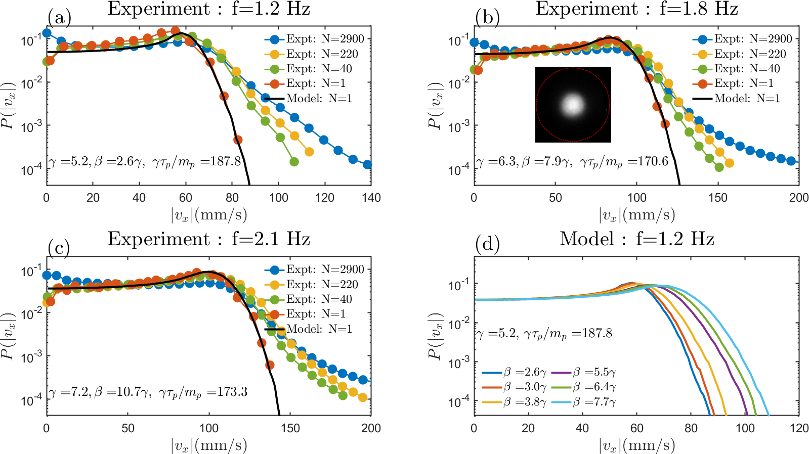
With each hysteretic transition, a certain amount of kinetic energy is lost. It would thus be natural to expect higher particle density to result in higher frictional dissipation and hence, lower velocities. However, contrary to this, we observe in Fig. 5 (a), (b) and (c) the tail of the velocity distribution , with , to increase with the density.
2.4 Model
There is as yet no agreement on the value of , with different experiments showing different values, e.g., references [41, 42] report as an universal parameter, while other experiments [43, 44, 45, 46] find to depend on system parameters, where could take on values close to 2. There exists multiple models to explain this deviation, e.g., presence of clustering [47], non-uniformity of granular temperature [48, 49], nature of noise injected by the drive [50, 49]. In most experiments, the strength of the noise is assumed to be a parameter controlled externally, e.g., energising a shaker more injects more noise to a granular gas, and it is assumed to be independent of the density of the particles. In the present situation, noise is injected when the particle toggles its state. Thus, with increasing density, the toggling increases in ways that are described in Fig. 4, and, hence, the strength of the noise increases.
In our model dynamics Eq. (5), which we now invoke as an effective single-particle dynamics to describe qualitatively the features observed in our experiment, the parameter parameterizes the frequency of this toggling. The model does well in reproducing the single particle velocity distribution functions for different values of the drive frequency. The data obtained from the numerical model are shown as black lines in Fig. 5 (a-c). For the many particle case it is mainly the initial part of the tail that fits well with the data.
2.5 The uniqueness of the stationary state
We now provide justification for claiming that the stationary state obtained for the experiments mentioned in this paper is qualitatively different from that observed in other driven systems. There is a large class of driven systems where the energy injection happens at the boundary [51, 52, 53, 54, 55, 56, 57, 58, 59, 60, 45, 43, 46, 42], e.g., balls on an electromagnetic shaker vibrating vertically or balls in a sinusoidally driven boxes. The height gained by the ball increases with the increase in frequency of the shaker (provided the peak displacement of the shaker does not change with the frequency). This is qualitatively opposite to what we observe for the coin on the moving plate where coin’s displacement reduces with increasing frequency of the moving plate. It may be noted here that for the coin on the plate, the point of energy injection is not spatially separated from where the energy is dissipated. It is the point of contact with the plate through which the system gains energy through momentum transfer, and it is also the same point through which energy is dissipated via friction. Similarly, the velocity distribution obtained for the spheres on the orbital shaker is also qualitatively different from that obtained in other experiments involving vibrated granular materials. For most low density systems, the tail of the velocity distribution varies as . There is a large spread in the value of reported in literature ranging from to . In contrast, we find that for the present method of driving, the tail of the velocity distribution has an exponential decay, i.e., . Moreover, the strength of the tail grows with increasing density.
Conclusion
In conclusion we first summarize the main experimental findings of the paper, then enumerate the salient features and the assumptions inherent in developing the state dependent driving model of the systems and comment on the success and shortcomings of the model.
Experiments:
Across all the three experiments we find the following essential features. (i) Abrupt alterations in the dynamics are associated with toggling of the frictional state. (ii) The tail of the velocity distribution has an exponential nature. In the context of many-particle systems, this tail gains weight with increasing density.
Model:
We have constructed a one-particle theoretical model that captures the essence of the experimental findings. Within our model, we treat the injection of energy into the system to be dependent on its dynamical state. In writing down the model we have made the following assumptions.
-
1.
We have treated the frictional coupling parameter as a stochastic variable whose togging in time is taken to be a Markov process that has two states; on () and off (). This Markovian assumption is a simplification of the underlying frictional process that is known to have memory associated with it.
-
2.
There is a single time scale in the problem given by the constant parameter whose inverse sets the time scale of toggling between the frictional states.
-
3.
In absence of a microscopic model that establishes the functional dependence between the and , we have chosen both to linearly vary with .
In spite of these assumptions, we find that our state dependent energy injection model does well in capturing the features of the experiments that are enumerated above. However in terms of exact matching this model leaves room for further improvement for many particle systems, see Fig. 5, panels (a)-(d), by, e.g., relaxing the assumptions mentioned above.
Systems with multiple components maintain themselves in a stable state by constantly regulating energy flow and dissipation, e.g., homeostasis in a biological setting is maintained by constant regulation of chemical processes, a governor in a combustion engine uses the inertial forces acting on it to limit the fuel injection. In physical terms, one can think of the system to be consisting of two parts, the body and the environment. The body is the place where the energy is dissipated and to maintain the processes in the body energy has to flow from the environment to the body. The rate of dissipation is a function of the inward energy flux and by controlling this flux, the body maintains a desired stationary state. Though such self-sustained stationary states are common to biological, chemical and system science settings, there seems to be a gap in realizing this regulation process in a more prosaic physical setting, particularly in situations where the energy injection and dissipation processes are clearly identified. In this paper, we have shown that for multiple experimental settings that span from a single particle to multiple particles, a state-dependent energy injection process can lead to a nontrivial stationary state in driven frictional systems. This stationary state is maintained by continued toggling between the different frictional states of the system. The energy injected to any of these states is a function of the state itself. We also provide a simple single parameter theoretical description of the various experimental realizations. Our work provides a new paradigm for finding routes to achieve non-equilibrium stationary states. It is only natural that future work in this direction would be to understand the conditions under which the stationary-state is maintained and the processes by which a given stationary state becomes unstable and a new stationary state is arrived at. This could possibly open new avenues to understand modes of failure leading to destabilization in complex systems.
Method
Experiment 1: A brass coin of diameter is placed on a groove on an aluminum plate. The groove has length and a thickness slightly larger than the diameter of the coin so that the coin is restricted to move in the direction only. The plate is kept on top of a shaker executing simple harmonic motion in the direction, see Fig. 1(a). The amplitude of the vibration () is . The motion of both the coin and the plate is observed simultaneously at from a camera fixed in the laboratory frame for a duration of . The coefficient of static friction measured between the coin and the plate is . The critical frequency below which the coin is completely stuck to the plate is calculated to be . Image processing is done in Matlab. We have done the experiments for other pairs of materials namely Aluminium coin on Aluminium plate, Acrylic coin on Aluminium plate and Acrylic coin on Acrylic plate. The experimental results as well as the results from numerical simulation for these pairs are provided in appendix.
Experiment 2: A single stainless steel ball of diameter is confined on an cylindrical container of diameter and height made of anodized aluminum, with a glass plate used as a lid for the container to enforce a two-dimensional geometry for the problem. The container is placed on a square platform, and the entire assembly along with a camera (used for imaging) is made to perform an orientation-preserving horizontal circular motion (orbital motion). The amplitude of the circular motion () is . Images are captured at at a resolution of for a duration of . Image processing is done in Matlab and ImageJ.
Experiment 3: number of stainless steel balls are placed on the same setup as Experiment 2. Particle tracking is done by using the algorithm mentioned in [61].
Appendix A Appendices
A.1 Coin on a moving plate : Comparison between experimental and numerical results across different pairs of materials.
At the microscopic level, the toggling between the frictional states is determined by the formation and rupture of the contact zone between the particle and the moving plate. Thus the noise associated with the toggling is closely related to the dynamics of this contact zone (interface). For the contact to break a critical yielding stress of the contact zone needs to be exceeded. In the framework of rate-state model of friction, for the contact to break a critical slip length needs to be reached [32]. Within this model, is a linear function of the frictional coupling strength .
In general the coupling between the plate and the particle is viscoelastic [62, 63], and hence the frequency response of can be written in terms of the storage modulus () and loss modulus () as,
| (6) |
Here , and is the characteristic length scale of the coin. Within the framework of Maxwell’s model of viscoelasticity,
| (7) | |||||
| (8) |
Here and are the zero-frequency viscosity and rigidity, respectively, and is the only relaxation time in the problem.
The following equation describes the motion of the particle (see the main paper for details).
| (9) |
For and we have
| (10) |
Here is the phase difference between the plate and the coin and which is a function of the toggling rate is the time averaged value of the dichotomous noise .
For values of ,
| (11) | |||||
| (12) |
In the limit of , we obtain a frequency weakening response of the frictional coupling , i.e., and = 0.
| (13) | |||||
| (14) | |||||
| (15) |
In this limit and . These observations are consistent with our experimental observations.
The stochasticity associated with the toggling process has its microscopic origin in the variation of the instantaneous value of the length at which the slip is initiated. This is closely related to the yielding process of the interface and hence the strength of the noise associated with this process should be proportional to the mechanical properties of the interface, thus should be a function of the frictional coupling that is described by .
| Coin on Plate | |||||||
|---|---|---|---|---|---|---|---|
| (Hz) | (kg/s) | (Hz) | (Hz) | ||||
| Brass on Aluminium | 4.4 | 12 | 2.2 | 10.7 | 238 | 1562 | 0.21 |
| Aluminium on Aluminium | 5.4 | 12 | 4 | 14 | 238 | 1562 | 0.45 |
| Acrylic on Aluminium | 5.15 | 55 | 55 | 7 | 222 | 2000 | 0.38 |
| Acrylic on Acrylic | 6 | 55 | 55 | 3 | 1250 | 500 | 0.66 |
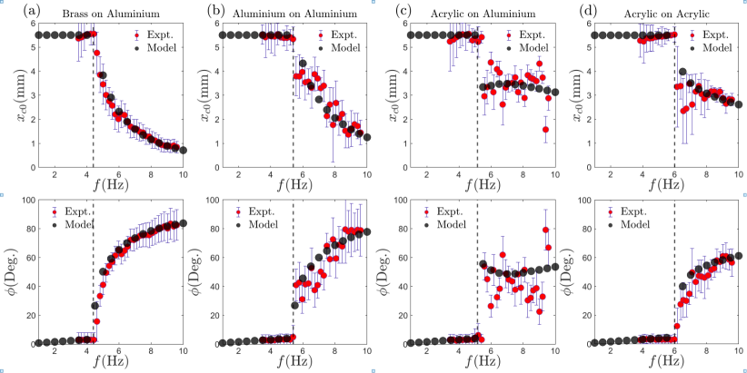
In absence of a microscopic model that establishes the functional dependence between the two, we have chosen both and to linearly vary with . Here is the reduced frequency of the drive and denotes the critical drive frequency beyond which the coin begins to slip. The choice of this linear variation was necessitated to account for the strain rate induced weakening of the frictional coupling. We take the following functional forms of the parameters and to describe their dependence on the drive frequency .
| (16) | |||||
| (17) |
Moreover, the dimensionless parameter
was taken to be a constant whose value depends on the pair of the material involved in the frictional process. The comparison between the results obtained from the simulation and the experiments across different pairs of coin and the plate materials is provided in Fig. 6. These results also highlight the contrasting frictional response of pairs involving hard (metals, Gpa, GPa) materials and those involving softer (polymethyl methacrylate (Acrylic), GPa) materials. Hard materials with larger values of elastic constant have larger critical slip lengths and hence are less prone to frictional instabilities, these materials exhibit a continuous type of transition across . In contrast, the pairs involving acrylic (a softer material that lower rigidity modulus and hence small critical slip length ) are more prone to frictional instabilities and hence exhibit an abrupt jump across the transition. These features are captured well within the model. The comparison of the experimental findings with that obtained from the model are provided in Fig. 6 for different pairs of materials.
A.2 Predictions from the Coloumb Model
In performing the simulations for the Coulomb friction model [18] we have assumed . The simulated velocity profile is shown in Fig. 7(a). It can be noted that there are discontinuous jumps in the velocity plot marked as dotted lines. This happens because of the presence of the velocity gap in the coulomb friction model associated with the transition of the coin from the slip state to the stuck state as pointed out in section on “Dry friction models and their limitations” of the main paper. The corresponding velocity distribution of the coin is plotted in Fig. 7(b) (blue dots). As a reference the velocity distribution of the plate is also plotted alongside (red dots). Since the velocity of the coin is linear in time in the slip state, it corresponds to the constant part of the distribution function in Fig. 7(b). Whereas, in the stuck state the velocity of the coin follows that of the plate, which corresponds to the part which follows the increasing part of the distribution. A small part of the lower velocity range is absent in the velocity distribution of the coin which falls in the velocity gap mentioned above. The amplitude and phase difference of the coin with respect to the plate are shown in Fig. 7(c) and (d) respectively. Clearly they do not agree with the experimental data.
Shamik Gupta acknowledges support from the Science and Engineering Research Board (SERB), India under SERB-TARE scheme Grant No. TAR/2018/000023, SERB-MATRICS scheme Grant No. MTR/2019/000560, and SERB-CRG scheme Grant No. CRG/2020/000596.
The authors Soumen Das and Shankar Ghosh thank Prajwal Panda, Anit Sane and Soham Bhattacharya for their help in the experiments.
References
- [1] Malthe-Sørenssen A 2021 Nature Physics 17 983–985
- [2] Svetlizky I and Fineberg J 2014 Nature 509 205–208
- [3] Kumar D, Nitsure N, Bhattacharya S and Ghosh S 2015 Proceedings of the National Academy of Sciences 201500665
- [4] Das S and Ghosh S 2020 Physical Review Research 2 013142
- [5] Livi R and Politi P 2017 Nonequilibrium statistical physics: a modern perspective (Cambridge University Press)
- [6] Aumaître S, Schnautz T, Kruelle C A and Rehberg I 2003 Physical Review Letters 90 114302 ISSN 0031-9007, 1079-7114 URL http://link.aps.org/doi/10.1103/PhysRevLett.90.114302
- [7] Tailleur J and Cates M 2008 Physical review letters 100 218103
- [8] Golestanian R and Ajdari A 2008 Physical review letters 100 038101
- [9] Jee A Y, Dutta S, Cho Y K, Tlusty T and Granick S 2018 Proceedings of the National Academy of Sciences 115 14–18
- [10] Pennestrì E, Rossi V, Salvini P and Valentini P P 2016 Nonlinear dynamics 83 1785–1801
- [11] Ghosh S, Merin A and Nitsure N 2017 Journal of Physics: Condensed Matter 29 355001
- [12] Stelter P 1992 Nonlinear dynamics 3 329–345
- [13] Denny M 2004 European journal of physics 25 311
- [14] Urbakh M, Klafter J, Gourdon D and Israelachvili J 2004 Nature 430 525–528
- [15] Schwarz U D and Holscher H 2016 ACS nano 10 38–41
- [16] Popov V L and Gray J 2014 Prandtl-tomlinson model: a simple model which made history The history of theoretical, material and computational mechanics-mathematics meets mechanics and engineering (Springer) pp 153–168
- [17] Vanossi A, Manini N, Urbakh M, Zapperi S and Tosatti E 2013 Reviews of Modern Physics 85 529
- [18] Persson B N 2013 Sliding friction: physical principles and applications (Springer Science & Business Media)
- [19] Krylov S Y, Jinesh K, Valk H, Dienwiebel M and Frenken J 2005 Physical Review E 71 065101
- [20] Gnecco E and Meyer E 2015 Fundamentals of Friction and Wear on the Nanoscale (Springer)
- [21] Braun O M, Kivshar Y and Kivshar Y S 2004 The Frenkel-Kontorova model: concepts, methods, and applications (Springer Science & Business Media)
- [22] Peyrard M and Aubry S 1983 Journal of Physics C: Solid State Physics 16 1593
- [23] Sándor B, Járai-Szabó F, Tél T and Néda Z 2013 Physical Review E 87 042920
- [24] Abe Y and Kato N 2014 Nonlinear Processes in Geophysics 21 841–853
- [25] Carlson J M and Langer J 1989 Physical Review Letters 62 2632
- [26] Gagnon L, Morandini M and Ghiringhelli G L 2020 Archive of Applied Mechanics 90 107–126
- [27] Buguin A, Brochard F and De Gennes P G 2006 The European Physical Journal E 19 31–36
- [28] Müser M H 2008 Proceedings of the National Academy of Sciences 105 13187–13188
- [29] Li Q, Tullis T E, Goldsby D and Carpick R W 2011 Nature 480 233–236
- [30] Albertini G, Karrer S, Grigoriu M D and Kammer D S 2021 Journal of the Mechanics and Physics of Solids 147 104242
- [31] Feng Q 2003 Computer methods in applied mechanics and engineering 192 2339–2354
- [32] Dieterich J H 1979 Journal of Geophysical Research: Solid Earth 84 2161–2168
- [33] Ruina A 1983 Journal of Geophysical Research: Solid Earth 88 10359–10370
- [34] Van den Ende M, Chen J, Ampuero J P and Niemeijer A 2018 Tectonophysics 733 273–295
- [35] Tian K, Goldsby D L and Carpick R W 2018 Physical review letters 120 186101
- [36] Baumberger T, Berthoud P and Caroli C 1999 Physical Review B 60 3928
- [37] Scholz C H 2019 The mechanics of earthquakes and faulting (Cambridge university press)
- [38] Uenishi K and Rice J R 2003 Journal of Geophysical Research: Solid Earth 108
- [39] Scherer M A, Kötter K, Markus M, Goles E and Rehberg I 2000 Physical Review E 61 4069
- [40] Aumaitre S, Kruelle C and Rehberg I 2001 Physical Review E 64 041305
- [41] Losert W, Cooper D, Delour J, Kudrolli A and Gollub J 1999 Chaos: An Interdisciplinary Journal of Nonlinear Science 9 682–690
- [42] Rouyer F and Menon N 2000 Physical review letters 85 3676
- [43] Kudrolli A and Henry J 2000 Physical Review E 62 R1489
- [44] Van Zon J and MacKintosh F 2004 Physical review letters 93 038001
- [45] Olafsen J and Urbach J S 1999 Physical Review E 60 R2468
- [46] Blair D L and Kudrolli A 2001 Physical Review E 64 050301
- [47] Van Noije T and Ernst M 1998 Granular Matter 1 57–64
- [48] Nie X, Ben-Naim E and Chen S 2000 EPL (Europhysics Letters) 51 679
- [49] Puglisi A, Loreto V, Marconi U M B and Vulpiani A 1999 Physical Review E 59 5582
- [50] Prasad V, Das D, Sabhapandit S and Rajesh R 2017 Physical Review E 95 032909
- [51] Kudrolli A, Wolpert M and Gollub J P 1997 Physical Review Letters 78 1383
- [52] Falcon É, Wunenburger R, Évesque P, Fauve S, Chabot C, Garrabos Y and Beysens D 1999 Physical review letters 83 440
- [53] Opsomer E, Ludewig F and Vandewalle N 2011 Physical Review E 84 051306
- [54] Noirhomme M, Cazaubiel A, Darras A, Falcon E, Fischer D, Garrabos Y, Lecoutre-Chabot C, Merminod S, Opsomer E, Palencia F et al. 2018 EPL (Europhysics Letters) 123 14003
- [55] Bougie J, Moon S J, Swift J and Swinney H L 2002 Physical Review E 66 051301
- [56] Meerson B, Pöschel T, Sasorov P V and Schwager T 2004 Physical Review E 69 021302
- [57] Eshuis P, Van Der Weele K, Van Der Meer D, Bos R and Lohse D 2007 Physics of Fluids 19 123301
- [58] Sack A, Heckel M, Kollmer J E, Zimber F and Pöschel T 2013 Physical review letters 111 018001
- [59] Clement E and Rajchenbach J 1991 EPL (Europhysics Letters) 16 133
- [60] Warr S, Huntley J M and Jacques G T 1995 Physical Review E 52 5583
- [61] Jaqaman K, Loerke D, Mettlen M, Kuwata H, Grinstein S, Schmid S L and Danuser G 2008 Nature methods 5 695–702
- [62] Prerna Sharma, Shankar Ghosh, and S Bhattacharya. Microrheology of a sticking transition. Nature Physics, 4(12):960–966, 2008.
- [63] Deepak Kumar, S Bhattacharya, and Shankar Ghosh. Weak adhesion at the mesoscale: particles at an interface. Soft Matter, 9(29):6618–6633, 2013.