State Constrained Stochastic Optimal Control for Continuous and Hybrid Dynamical Systems Using DFBSDE

The derivation presented in this section was originally proposed in [22], it is summarized here for completeness. Let $\mathbf{V}(\cdot,\cdot)$ be the value function $\mathbf{V}(\mathbf{x},t)\in\mathbb{R}_{+}$ defined as

Using (2) and Bellman’s principle [1] yields

where $\mathbf{h}$ denotes the Hamiltonian

the differential operator of $\mathbf{V}$ is given by

$\mathbf{V}_{t}(\mathbf{x},t)\in\mathbb{R}$ is the partial derivative of $\mathbf{V}$ with respect to $t$, and $\mathbf{V}_{\mathbf{x}}(\mathbf{x},t)\in\mathbb{R}^{n\times 1}$ and $\mathbf{V}_{\mathbf{x}\mathbf{x}}(\mathbf{x},t)\in\mathbb{R}^{n\times n}$ denote the first and second partial derivatives, respectively, of $\mathbf{V}$ with respect to $\mathbf{x}$. To consider control constraints [22], we define $\mathbf{r}(\mathbf{u})$ as

with $\mathbf{u}_{i}^{\max}$ being the $i$-th element of $\mathbf{U}_{\max}$ and

In (9), $c_{i}$ weights the importance between different control inputs. Using first-order conditions to solve for an analytic solution of the optimal control action that achieves the infimum of the Hamiltonian yields

with $\mathbf{R}=\mathrm{diag}(c_{1},\cdots,c_{m})$. Solving (11) for $\mathbf{u}^{*}$ in yields

with “$*$” denoting element-wise multiplication. The control is saturated between $[-\mathbf{U}_{\max},\mathbf{U}_{\max}]$. Define $\mathbf{y}(t)=\mathbf{V}(\mathbf{x}(t),t)$. From (7), we can write a stochastic system for the optimal value function

which is in the form of a FBSDE (the forward part consists of (13b) (13d), the backward part consists of (13a) (13c)). The forward and backward parts are of the form of a forward SDE (FSDE) and a backward SDE (BSDE), respectively. For details regarding the derivation from (7) to (13), the reader is referred to [22][6].

In this section, we consider incorporating state constraints into the FBSDE framework using a penalty function based approach. A perfect penalty function would be zero inside the constraint boundary and infinity outside. We propose two differentiable and numerically stable alternatives to a perfect penalty function. The first option is a penalty function based on logistic functions (PFL). When the state constraint has both an upper bound $\mathbf{b}_{\max}$ and lower bound $\mathbf{b}_{\min}$, the $i$-th element of PFL would be

where $L\in\mathbb{R}^{+}$ determines the maximum value of the penalty, $\mathbf{k}\in\mathbb{R}^{+}$ determines the steepness of the boundary (larger $k$ leads to steeper boundaries), and $\mu=(\mathbf{b}_{\min}+\mathbf{b}_{\max})/2$. The proposed penalty function consists of two parts: the first consists of two logistics functions, which give the valley shape; the second sets the minimum value of the penalty function to zero. The second option is a rectified-linear-unit (ReLU) based function which is defined as $\mathbf{ReLU}(x)=\max(x,0)$. When an upper and lower bound exist, the penalty function is

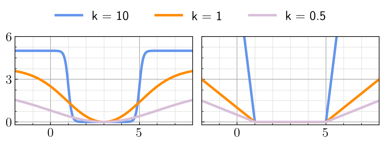
Similar to (3.2), $\mathbf{k}$ represents steepness of the constraint boundaries. However, in (3.2), there is no bound on the penalty function magnitude. An example of these two types of penalty functions with varying steepness is shown in Fig. 1. When only an upper bound exists, i.e., $\mathbf{c}(\mathbf{x})\leq\mathbf{b}$, the lower bound is set to be $-\infty$, and when only a lower bound exists, i.e., $\mathbf{c}(\mathbf{x})\geq\mathbf{b}$, the upper bound is set to be $\infty$. The main difference between these two penalty functions is their values within the constraint boundary. For PFL, the value of the penalty function is only close to zero when a large $\mathbf{k}$ value is utilized. Otherwise, states within but close to constraint boundaries will have a positive penalty function value. The ReLU-based penalty function is always zero within the bound. Specific use cases are demonstrated in Section 4. After applying penalty function $\mathbf{p}(\mathbf{x})$, the instantaneous state cost is $\bar{\mathbf{q}}(\mathbf{x})=\mathbf{q}(\mathbf{x})+\mathbf{p}(\mathbf{x})$. Ideally, we would pick larger $\mathbf{k}$ and $L$ to ensure a steeper boundary and larger penalty. While a controller without access to measurements of future noise can not guarantee that state constraints will be met for all time due to stochastic nature of the system dynamics, note that the penalty functions guide the learning towards a robust controller that does not violate state constraints (at least under the disturbances seen during training). The expected value of the integral of $\mathbf{p}(\mathbf{x})$ is at most $J^{\mathbf{u}}$. If $J^{\mathbf{u}}$ is finite and $\mathbf{p}(\mathbf{x})$ is a perfect penalty function, the constraint is satisfied except on a set of measure zero.

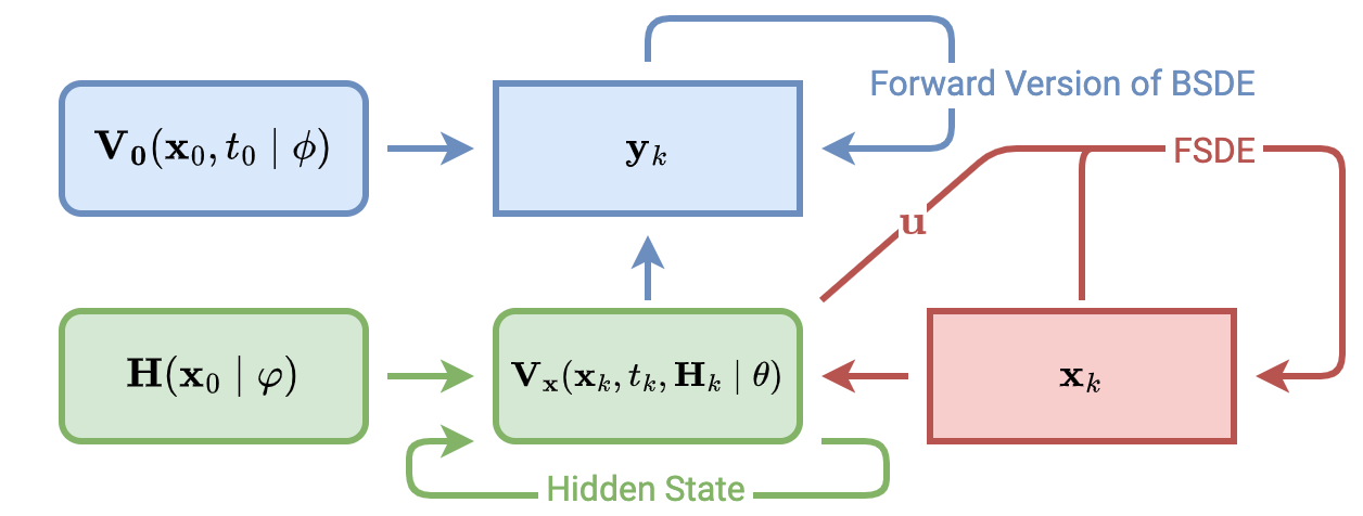
The solution of the FBSDE in (13) requires backward integration in time and the fact that $\mathbf{V}_{\mathbf{x}}(\mathbf{x})$ is unknown creates additional difficulties in utilizing classical numerical integration approaches. To deal with backward integration in time, following the formulation in [22], we can estimate the value function at time zero using a DNN, which is parameterized by $\phi$, i.e., $\mathbf{V}_{\mathbf{0}}(\mathbf{x},t_{0})$. This allows the forward integration of the BSDE. We can then rewrite the FBSDE as two FSDEs. For unknown $\mathbf{V}_{\mathbf{x}}(\mathbf{x},t)$ values, it can also be estimated using a DNN parameterized by $\theta$, i.e., $\mathbf{V}_{\mathbf{x}}(\mathbf{x},t\mid\theta)$. We deploy an LSTM-based architecture [13] for $\mathbf{V}_{\mathbf{x}}(\mathbf{x},t\mid\theta)$, which has been shown to be superior to dense-layer-based architectures [22]. Linear regression based approaches have also been considered, but are inferior due to compounding error. Assuming the initial state and time horizon are fixed [22], the initial value function is a learned fixed value $\mathbf{V}_{\mathbf{0}}(\phi)$. Due to the use of LSTMs, two changes need to be made to the DFBSDE algorithm. First, a separate network $\mathbf{H}_{0}(\varphi)$ is used to estimate the initial hidden state values. Second, $\mathbf{y}_{k}$ will also depend on the hidden state values $\mathbf{H}_{k}$. The FBSDE can be forward integrated by discretizing the time as follows

where $k\geq 1$, $\Delta{t}=T/N$, $\Delta{\mathbf{x}}_{k}=\dot{\mathbf{x}}(k\Delta{t})\Delta{t}$ and $\Delta{\mathbf{w}}_{k}=\dot{\mathbf{w}}(k\Delta{t})\Delta{t}$. The calculation of $\mathbf{x}_{k}$ and $\mathbf{y}_{k}$ is illustrated in Fig. 2. To learn the weights, we minimize the least square loss between the estimated terminal value function and the measured terminal cost,

where $M$ is the batch size and the superscript $j$ denotes the $j$-th set of data in the batch. The detailed DFBSDE algorithm is shown in Algorithm 1.

For the penalty function, if $\mathbf{k}$ is set to a large value in the initial stage of training, numerical instabilities can arise due to large gradients generated by states within the steep region near the constraint boundary. On the other hand, if the values of $\mathbf{k}$ are kept small, it would not be effective since the penalty for constraint violation is small. Thus, we propose to update $\mathbf{k}$ during training so that it gradually increases. The update scheme is as follows. For a given $\mathbf{k}$, the DNN is trained until convergence; then, $\mathbf{k}$ is updated. A metric to check for convergence is the variance of the episode-wise cost over a few episodes; the episode window size is denoted as $\eta$. If the iterates are converging, the variance will be small. Convergence is determined by comparing the square root of the variance with a threshold $\beta\in\mathbf{R}_{+}$; if it is smaller than $\beta$, $\mathbf{k}$ is updated as $\mathbf{k}\leftarrow\mathbf{k}+\delta$. This condition is checked every $\eta$ iterations. Additionally, if the condition is not satisfied after $\eta^{\prime}$ iterations, then also $\mathbf{k}$ is updated since it could be stuck at a local minimum. Empirically, we have found $\eta=500$, $\mathbf{k}=1.5$, $\delta=0.5$, and $\Delta_{\delta}=0.25$ to be reasonable values to start with. Both $\delta$ and $\Delta_{\delta}$ can be increased if training is stable and faster growth of $\mathbf{k}$ is desired; otherwise, $\delta$ and/or $\Delta_{\delta}$ should be reduced. During training, the variance decreases. Thus, $\beta$ should also decrease after each update: $\beta=\gamma\beta$, with $\gamma\in(0,1)$. To make the decrease in $\beta$ smoother, we gradually increase $\gamma$ to 1 using $\gamma=\gamma+\Delta$ with $\Delta\in\mathbb{R}_{+}$. Similarly, the acceleration of $k$ is made negative, i.e., $\delta=\delta+\Delta_{\delta}$, with $\Delta_{\delta}\in\mathbb{R}_{-}$, leading to finer-grained changes in $k$ at later stages of training. The initial value of $\beta$ can be determined after the training converges for the first iteration of Algorithm 2. From empirical evaluations, we find $\gamma=0.9$ and $\Delta=0.02$ to be reasonable values. The penalty function update scheme is shown in Algorithm 2.

This section will discuss the adaptations required for the DFBSDE algorithm to handle HD systems. HD systems consist of two phases: a continuous dynamic phase and a phase of a deterministic discrete jump. Such an HD system is very common, e.g., a biped. The FBSDE formulation in (13) is only for continuous dynamics. Inspired by the cyclic motion in human walking, we treat the hybrid dynamics as having multiple cycles, where the dynamics are continuous within each cycle. For the case of bipedal locomotion, each cycle will be a footstep; at the end of each cycle, the swing foot lands on the ground (more on this in Section 4). The main challenges in adapting the DFBSDE framework to HD systems are robustness to the initial state and assurance of cyclic motion. This requires the initial value function estimator to be robust to a wide range of states. The loss function (17) only trains the estimator for a fixed $\mathbf{x}_{0}$. To ensure that the learned value function estimator is robust to variations in the initial state, we can train it such that it provides an accurate estimation for all of the states recorded. The measured cost-to-go can approximate the value function

Using (18), we can learn the initial value function using

Thus, the loss function for the Hybrid FBSDE (HFBSDE) becomes

with the terminal cost calculated using the state after the jump $\mathbf{x}_{N}^{+}$ and $\lambda\in\mathbb{R}_{+}$ adjusts the weighting between the two losses. This terminal cost encourages cyclic motion.

The task for the cart-pole system is to swing the pole up and stabilize it at the top. The cart-pole dynamics are

The cart position and pendulum angle are represented by $x$ and $\theta$, respectively. The pendulum angle is zero when it is pointed downwards. The state of the cart-pole system is $[x,\ \theta,\ \dot{x},\ \dot{\theta}]^{T}$. In our experiments, we set the cart mass to $M=1.0$kg, the pole mass to $m=0.01$kg (point mass at the tip), the pole length to $\ell=0.5$m, $\mathbf{x}_{0}=\mathbf{0}_{4\times 1}$, and the target state as $[0,\pi,0,0]^{T}$. The control is saturated at $\pm 10$N, the cart position is constrained between $\pm 1.5$m, and the cart velocity is constrained between $\pm 2.5$m. The time horizon is chosen to be $2.5$ sec and the time step is $\Delta{t}=1/110$ sec (this specific value of $\Delta{t}$ is chosen randomly). We use the state cost function

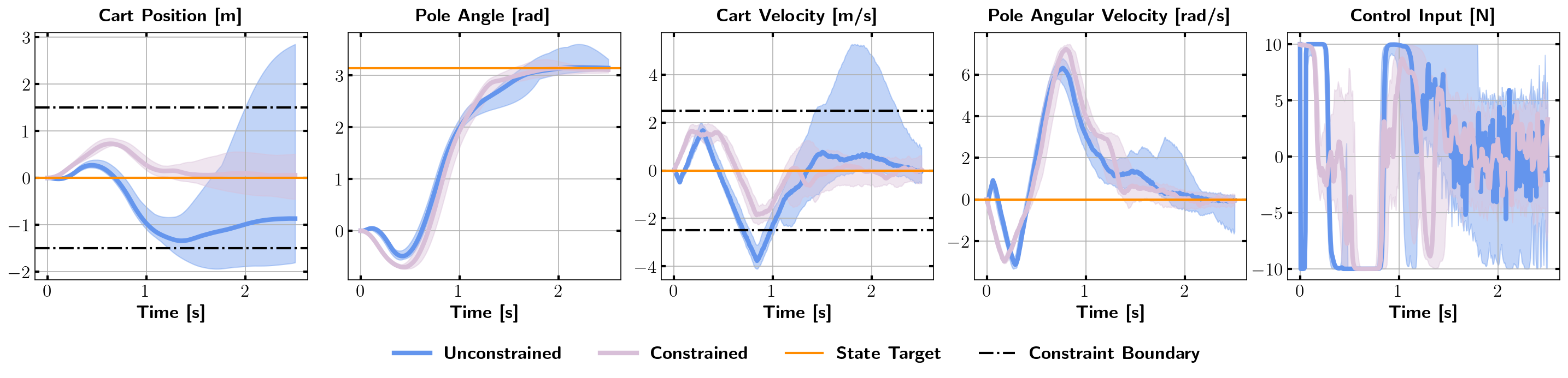
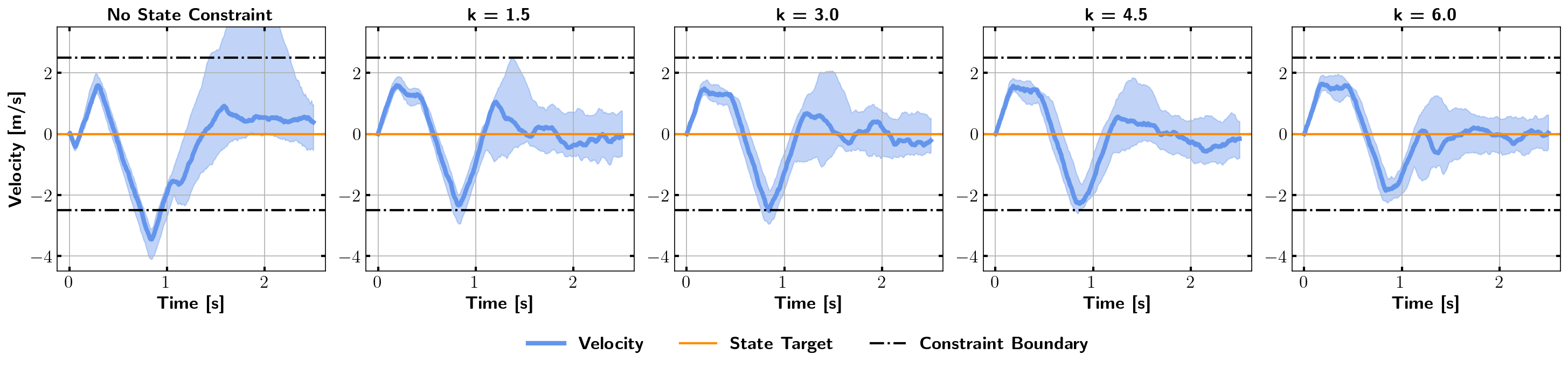
where $\bar{\mathbf{x}}$ is the target state, $\mathbf{Q}$ is the cost weight matrix for the state, and $\mathbf{Q}_{N}$ is the terminal state cost matrix. We use the control cost defined in (9). The cost matrices are chosen as $\mathbf{Q}=\mathbf{Q}_{N}=\mathrm{diag}([0.5,\ 1.0,\ 0.1,\ 0.1])$ and $\mathbf{R}=[0.1]$. $\mathbf{p}(\cdot)$ is the penalty function, in this example $\mathbf{p}(\cdot)$ is a logistics function-based penalty function (3.2), with $\mathbf{c}(\mathbf{x})=[x,\dot{x}]^{T}$ and $\mathbf{b}_{\max}=-\mathbf{b}_{\min}=[1.5,2.5]^{T}$. Fig. 3 shows the state trajectories generated by the trained controller. The state trajectory generated by the trained constrained DFBSDE controller satisfies the state constraints, while they are violated significantly under the trained unconstrained controller. The effect of the penalty function can be immediately seen in Fig. 4, even with a small $k$ value. With $k=1.5$, the part of the trajectory that lies outside the constraint boundaries is greatly reduced. After gradually increasing $k$ to $6.0$, following Algorithm 2, the entire cart velocity trajectory lies within the constraint boundaries. We also tested directly training with $k=6.0$ without the adaptive update. The algorithm becomes numerically unstable after one epoch due to large gradients. This demonstrates that our method provides a stable training scheme.

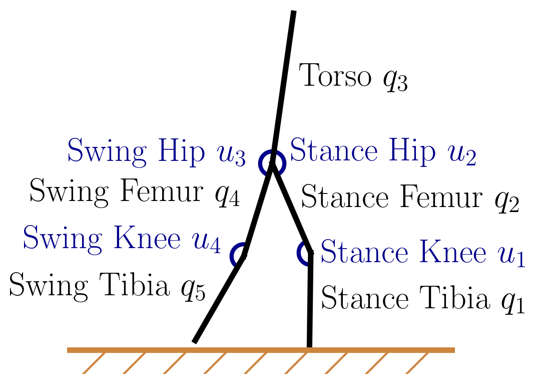
The biped model of interest is shown in Fig. 5, derived from [3]. The leg on the ground is the stance leg, the leg in the air is the swing leg, and the link representing the upper body is the torso. The biped state $\mathbf{x}\in\mathbb{R}^{10\times 1}$ consists of the link angles with respect to the horizontal plane $\mathbf{q}\in\mathbb{R}^{5\times 1}$ and the link angular velocities $\dot{\mathbf{q}}\in\mathbb{R}^{5\times 1}$, i.e., $\mathbf{x}=[\mathbf{q}^{T},\ \dot{\mathbf{q}}^{T}]^{T}$. Note that the $\mathbf{q}$ denoted here is different from the state cost function $\mathbf{q}(\mathbf{x})$. The biped model has four actuated joints at the knee and hip joints. The control $\mathbf{u}\in\mathbb{R}^{5\times 1}$ consists of the applied torque at the actuated joints $\mathbf{u}=[0,\ u_{1},\ u_{2},\ u_{3},\ u_{4}]^{T}$, where the $0$ corresponds to the unactuated stance ankle. The output of the controller will only consist of $\tilde{\mathbf{u}}=[u_{1},\ u_{2},\ u_{3},\ u_{4}]$, then a mapping matrix $T=[\mathbf{0},\ \mathbf{I}_{4\times 4}]$ is used to obtain $\mathbf{u}=T\tilde{\mathbf{u}}$. The parameters of the biped model can be found in [15]. The five-link biped dynamics is

where $\mathbf{M}(\mathbf{q})\in\mathbb{R}^{5\times 5}$ is the inertia matrix, $\mathbf{C}(\mathbf{q},\dot{\mathbf{q}})\in\mathbb{R}^{5\times 5}$ the Coriolis matrix, and $G(\mathbf{q})\in\mathbb{R}^{5\times 1}$ the gravitational terms. The dynamics is in the form of (1) after considering stochastic noise. A heel strike (HS) occurs when the biped comes into contact with the ground, which signals the termination of the current step, and initiation of the next step. During this transition, the swing and stance legs are swapped. We assume this transition is instantaneous, the biped is symmetric, and the new swing leg leaves the ground once the HS occurs (i.e., no double support phase). The joint indexing depends on the current swing and stance leg definition. Defining the joint angles right before HS as $\mathbf{q}^{-}\in\mathbb{R}^{5\times 1}$ and the joint angles right after HS as $\mathbf{q}^{+}\in\mathbb{R}^{5\times 1}$, we have $\mathbf{q}^{+}=\tilde{\mathbf{I}}_{5\times 5}\mathbf{q}^{-}$, where $\tilde{\mathbf{I}}_{5\times 5}\in\mathbb{R}^{5\times 5}$ is the anti-diagonal matrix. The HS creates an instantaneous change in angular velocity. Defining the angular velocity before HS as $\dot{\mathbf{q}}^{-}\in\mathbb{R}^{5\times 1}$ and the angular velocity after HS as $\dot{\mathbf{q}}^{+}\in\mathbb{R}^{5\times 1}$, we have $\mathbf{x}^{+}=\mathbf{f}_{H}(\mathbf{x}^{-})$, with $\mathbf{f}_{H}:\mathbb{R}^{10\times 1}\rightarrow\mathbb{R}^{10\times 1}$ being the deterministic HS transition map [15].

To generate realistic walking motion, we need to avoid hyperextension in the knee. We transform this constraint into a variant of the ReLU-based penalty function in (3.2): $\mathbf{p}(\mathbf{x})=\alpha\mathbf{ReLU}(-(q_{4}-q_{5}))$ where $\alpha$ is a weighting coefficient for the penalty function, and $q_{4}$ and $q_{5}$ are defined in Fig. 5. A quadratic cost is applied to the control. We choose $\mathbf{R}=\mathrm{diag}([2,\ 0.2,\ 0.2,\ 2])$. This choice of $\mathbf{R}$ implies that hip motors are more powerful than knee motors, which is true for many robots. The state cost $\mathbf{q}(\mathbf{x})$ is the weighted distance between the state $\mathbf{x}$ and a nominal terminal state $\bar{\mathbf{x}}$ plus the penalty

with $\mathbf{Q}=10\mathbf{I}_{10\times 10}$. The terminal state cost has the same form as (25), the sole difference is replacing the state cost matrix with $\mathbf{Q}_{N}=10\mathbf{Q}$. The target state is chosen to be

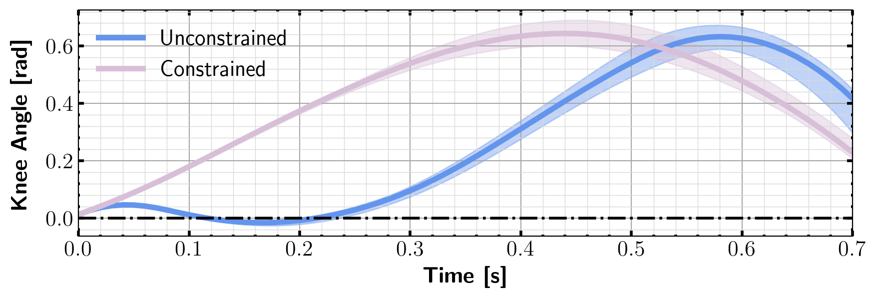
A comparison between the motion generated by the constrained and unconstrained DFBSDE controller is given in Fig. 6. The unconstrained controller hyperextends the swing knee, while the constrained controller does not. Since the chosen penalty function could constrain the system directly, the $k$ value doesn’t need to be updated. In previous examples, the penalty functions are logistic function based. This works well when the constraint set is large since it creates a buffer between the interior of the constraint set and its boundary. However, the constraint set for locomotion tasks is relatively small, making ReLU functions a better candidate. For the five-link biped experiments, we use a time step of 0.01s.

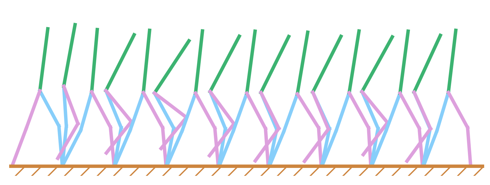
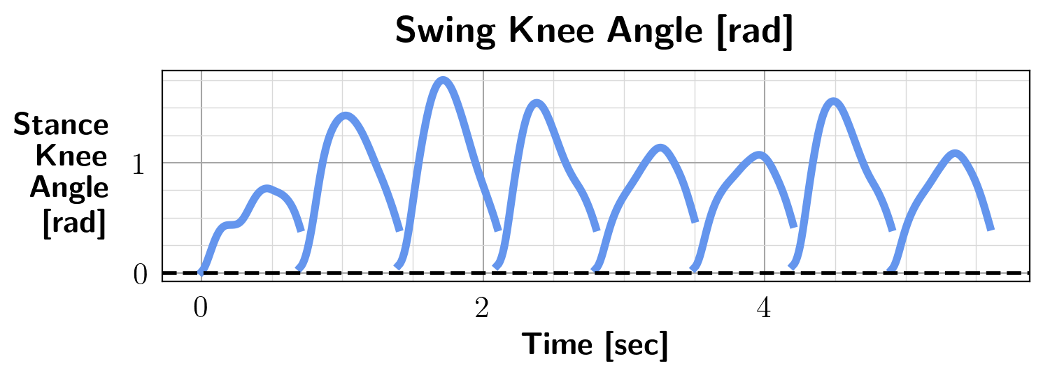
Variations in the initial states make dissecting a multi-step walking problem into multiple single-step walking problems a challenging task. We train a robust controller to deal with this issue. We find it difficult for a single controller to handle all possible initial configurations. Thus, we use an ensemble of controllers, where each controller handles a range of initial configurations around a nominal state. For the duration of one footstep, only one controller is used, which is the controller in the ensemble that has the shortest distance between the initial state and its nominal state. The nominal state of a controller is known a priori. After training, the motion generated by this approach is shown in Fig. 7, where the ensemble size is three. The corresponding swing knee angle is shown in Fig. 6. It can be seen that no hyperextension occurred, which shows the effectiveness of enforcing the state constraints. On average, the initial range each controller can handle spans 6.03 deg for the joint angles and 19.01 deg/sec for the joint velocities. Fig. 7 shows a tucking motion generated by the torso and the swing leg. This is due to our biped model’s relatively small control authority over the torso. Without the forward angular momentum generated by the tucking motion, the torso gradually tilts back over multiple steps. Since there is no direct control over the torso, it is difficult for the DFBSDE controller to recover. We also compared the computation time of our proposed method for obtaining the control for one time step with trajectory optimization [15] (TO). As expected, our approach generates comparable results while being computationally more efficient. Solving for the control action requires 0.96s for a Hermite-Simpson TO approach, compared with 5.6ms for our proposed method.

References

- [1] R.E. Bellman. Dynamic programming. Dover, New York, 2003.
- [2] Y. Chen, Y. Shi, and B. Zhang. Optimal control via neural networks: A convex approach. In Proceedings of International Conference on Learning Representations, New Orleans, LA, May 2019.
- [3] C. Chevallereau, G. Abba, Y. Aoustin, F. Plestan, E.R. Westervelt, C. Canudas-De-Wit, and J.W. Grizzle. RABBIT: a testbed for advanced control theory. IEEE Control Systems Magazine, 23(5):57–79, 2003.
- [4] L.G. Crespo and J. Sun. Stochastic optimal control via bellman’s principle. Automatica, 39(12):2109–2114, 2003.
- [5] B. Dai, P. Krishnamurthy, and F. Khorrami. Learning a better control barrier function. In Proceedings of IEEE Conference on Decision and Control, Cancun, Mexico, pages 945–950, December 2022.
- [6] B. Dai, P. Krishnamurthy, A. Papanicolaou, and F. Khorrami. State constrained stochastic optimal control using LSTMs. In Proceedings of the American Control Conference, New Orleans, LA, pages 1294–1299, May 2021.
- [7] B. Dai, V.R. Surabhi, P. Krishnamurthy, and F. Khorrami. Learning locomotion controllers for walking using deep FBSDE. CoRR, abs/2107.07931, 2021.
- [8] Bolun Dai, Heming Huang, Prashanth Krishnamurthy, and Farshad Khorrami. Data-efficient control barrier function refinement. In Proceedings of the American Control Conference, San Diego, CA, May 2023. (To Appear).
- [9] Bolun Dai, Rooholla Khorrambakht, Prashanth Krishnamurthy, Vinícius Gonçalves, Anthony Tzes, and Farshad Khorrami. Safe navigation and obstacle avoidance using differentiable optimization based control barrier functions. CoRR, abs/2304.08586, 2023.
- [10] M. Demetriou and E. Bakolas. Navigating over 3d environments while minimizing cumulative exposure to hazardous fields. Automatica, 115:108859, 2020.
- [11] M. Diehl, H.J. Ferreau, and N. Haverbeke. Efficient numerical methods for nonlinear mpc and moving horizon estimation. Nonlinear model predictive control, pages 391–417, 2009.
- [12] L. Hewing and M.N. Zeilinger. Scenario-based probabilistic reachable sets for recursively feasible stochastic model predictive control. IEEE Control Systems Letters, 4(2):450–455, 2019.
- [13] S. Hochreiter and J. Schmidhuber. Long short-term memory. Neural Computation, 9(8):1735–1780, 1997.
- [14] R. Sinnet J. Grizzle, C. Chevallereau and A. Ames. Models, feedback control, and open problems of 3d bipedal robotic walking. Automatica, 50(8):1955–1988, 2014.
- [15] M. Kelly. An introduction to trajectory optimization: How to do your own direct collocation. SIAM Review, 59(4):849–904, 2017.
- [16] M. Lorenzen, F. Dabbene, R. Tempo, and F. Allgöwer. Stochastic mpc with offline uncertainty sampling. Automatica, 81:176–183, 2017.
- [17] M.N. Mistry, J. Buchli, and S. Schaal. Inverse dynamics control of floating base systems using orthogonal decomposition. In Proceedings of the IEEE International Conference on Robotics and Automation, Anchorage, AK, pages 3406–3412, May 2010.
- [18] M. Neunert, M. Stäuble, M. Giftthaler, C.D. Bellicoso, J. Carius, C. Gehring, M. Hutter, and J. Buchli. Whole-body nonlinear model predictive control through contacts for quadrupeds. IEEE Robotics and Automation Letters, 3(3):1458–1465, 2018.
- [19] M. Pereira, Z. Wang, I. Exarchos, and E.A. Theodorou. Safe optimal control using stochastic barrier functions and deep forward-backward sdes. In Proceedings of Conference on Robot Learning, Cambridge, MA, volume 155, pages 1783–1801, November 2020.
- [20] L. Di Persio and M. Garbelli. Deep learning and mean-field games: A stochastic optimal control perspective. Symmetry, 13(1):14, 2021.
- [21] J. Viereck and L. Righetti. Learning a centroidal motion planner for legged locomotion. In Proceedings of the IEEE International Conference on Robotics and Automation, Xi’an, China, pages 4905–4911, May 2021.
- [22] Z. Wang, M.A. Pereira, and E.A. Theodorou. Learning deep stochastic optimal control policies using forward-backward SDEs. In Proceedings of Robotics: Science and Systems XV, Freiburg im Breisgau, Germany, June 2019.