STAS: Spatial-Temporal Return Decomposition for Multi-agent Reinforcement Learning
Abstract
Centralized Training with Decentralized Execution (CTDE) has been proven to be an effective paradigm in cooperative multi-agent reinforcement learning (MARL). One of the major challenges is credit assignment, which aims to credit agents by their contributions. While prior studies have shown great success, their methods typically fail to work in episodic reinforcement learning scenarios where global rewards are revealed only at the end of the episode. They lack the functionality to model complicated relations of the delayed global reward in the temporal dimension and suffer from inefficiencies. To tackle this, we introduce Spatial-Temporal Attention with Shapley (STAS), a novel method that learns credit assignment in both temporal and spatial dimensions. It first decomposes the global return back to each time step, then utilizes the Shapley Value to redistribute the individual payoff from the decomposed global reward. To mitigate the computational complexity of the Shapley Value, we introduce an approximation of marginal contribution and utilize Monte Carlo sampling to estimate it. We evaluate our method on an Alice & Bob example and MPE environments across different scenarios. Our results demonstrate that our method effectively assigns spatial-temporal credit, outperforming all state-of-the-art baselines.
Introduction
In recent years, significant progress has been made in the field of cooperative multi-agent reinforcement learning, demonstrating its potential to solve diverse problems across several domains (Du et al. 2023), such as Real-Time Strategy games (Vinyals et al. 2019), distributed control (Busoniu, Babuska, and De Schutter 2008), and robotics (Perrusquía, Yu, and Li 2021). However, cooperative games present a considerable challenge known as the credit assignment problem, which involves determining each agent’s contribution using the centralized controller. Furthermore, real-world environments are complex and unpredictable, leading to long-term delayed and discontinuous rewards, and causing inefficiencies in the learning process. For instance, in the game of Go, the agent may not receive rewards until the outcome is determined. These nontrivial features pose significant challenges to existing methods that mainly rely on dense rewards to learn a policy that maximizes long-term returns. Additionally, the lack of dense rewards can make finding optimal solutions difficult, resulting in high variance during training and potential failure to complete the task.
Substantial progress has been made in solving the credit assignment problem, with notable approaches including QMIX (Rashid et al. 2020), QTRAN (Son et al. 2019), and SQDDPG (Wang et al. 2020a). However, these methods do not address delayed reward environments. Recently, several studies have focused on temporal return decomposition methods that aim to decompose the return on a temporal scale (Liu et al. 2019a; Ren et al. 2022; Arjona-Medina et al. 2019). These methods use a Markovian proxy reward function to replace environmental rewards, converting the delayed reward problem into a dense reward problem. Inspired by this progress, we consider addressing the challenge of sparse or delayed rewards in multi-agent tasks.
In this paper, we consider a new task called the spatial-temporal return decomposition problem, in which the algorithm must not only decompose the delayed episodic return to each time step but also assign credits to each agent according to their contribution. To solve this problem, we propose a novel approach called STAS, which establishes a connection between credit assignment and return decomposition. The Shapley value (Shapley 1997; Bilbao and Edelman 2000; Sundararajan and Najmi 2020) is a well-known concept for computing relationships in cooperative games, as it considers all possible orderings in which players could join a coalition and determines the average marginal contribution of each player across all possible orderings. Inspired by that, STAS first uses a temporal attention to analyze state correlations within episodes, providing essential information for calculating Shapley values. Then it employs spatial attention module that uses Shapley values to allocate global rewards based on each agent’s contribution. We also introduce a random masked mechanism to overcome the computational complexity of the Shapley value by simulating different coalitions. In the spatial-temporal return decomposition problem, pinpointing key frames and the most contributory agent is vital for clear rewards that highlight actions positively impacting the final goal. By using a dual transformer structure, STAS can identify key steps with the temporal transformer and use the spatial transformer to find the key agents. This enables STAS to obtain a Markovian reward, resulting in a better simulation of dense reward situations. Finally, with successfully decomposed delayed return, single-agent can be effectively trained using policies such as PPO (Schulman et al. 2017) or SAC (Haarnoja et al. 2018).
In summary, our contributions are three-fold. Firstly, we define the Spatial-Temporal Return Decomposition Problem and propose STAS, which connects credit assignment with return decomposition to solve the problem. Secondly, we introduce a dual transformer structure that utilizes a temporal transformer to identify key steps in long-time intervals and a spatial transformer to find the most contributory agents. We also leverage the Shapley value to compute the contribution of each agent and design a random masked attention mechanism to approximate it. Lastly, we validate our approach in a challenging environment, Alice & Bob, showing superior performance and effective cooperative pattern learning. Additionally, our method excels in general tasks in the Multi-agent Particle Environment (MPE), surpassing all baselines.
Related Work
Return decomposition. Return decomposition, or temporal credit assignment, seeks to partition delayed returns into individual step contributions. Earlier methods relied on naive principles, such as count-based (Gangwani, Zhou, and Peng 2020; Liu et al. 2019a) or return-equivalent contribution analysis (Arjona-Medina et al. 2019; Patil et al. 2022; Zhang et al. 2023). Han et al. (2022) remodeled the problem and divided the value network into a history return predictor and a current reward one as HC-decompostion. Ren et al. (2022) proposed a concise method to utilize Monte Carlo Sampling as a time step sampler to decrease the computing complexity as well as the high variance. Although She, Gupta, and Kochenderfer (2022) initially addressed sparse rewards in credit assignment, their method falls short in extremely delayed reward scenarios, with only terminal rewards at the trajectory’s end. More recently, Xiao, Ramasubramanian, and Poovendran (2022) utilized attention structure to expand the return decomposition to multi-agent tasks as well as assign the reward to each agent in an implicit way by an end-to-end model.
Credit assignment. Credit assignment methods can be divided into implicit and explicit methods. Implicit methods treat the global value and the local value as a whole for end-to-end learning. Earlier methods ((Sunehag et al. 2018; Rashid et al. 2020)) developed a network to aggregate the Q-values of each agent into a global Q-value based on additivity or monotonicity. Subsequent methods attempt to delve deeper into the characteristics of IGM to achieve more accurate estimation (Son et al. 2019; Wang et al. 2021) or employ other approaches such as Taylor expansion to estimate global value (Yang et al. 2020; Wang et al. 2020b).
On the other hand, explicit methods attempt to establish an explicit connection between the global value and local value, enhancing the interpretability of the model by introducing algebraic relationships. Foerster et al. (2018) compute each agent’s advantage with a counterfactual baseline, while Wang et al. (2020a) introduced Shapley value to calculate the contribution of each agent. Li et al. (2021) combined counterfactual baseline and Shapley value to calculate each agent’s contribution in different coalitions. Du et al. (2019) learns per-agent intrinsic reward functions to evade credit assignment issue. Explicit methods typically employ the Actor-Critic architecture, which allows us to observe the contribution of each agent to the global reward, but this may result in high computational complexity.
Preliminaries
Cooperative Multi-Agent Reinforcement Learning In a fully cooperative multi-agent task (Panait and Luke 2005), agents need to work independently to achieve a common goal. Usually it can be described as a tuple: . Let denote the set of agents. Denote the joint state space of the agents as and the joint action space of the agents as respectively. is the state transition function. At time step , let with each being the state from agent . Accordingly, let with each indicating the action taken by the agent . All agents will share a global reward from environment . is a discount factor and is the distribution of the initial state . The goal of the agents is to find optimal policies that achieve maximum global return, where and is the length of horizon.
Shapley Value Shapley value is a popular method for computing individual contributions in cooperative games (Shapley 1997; Bilbao and Edelman 2000; Sundararajan and Najmi 2020). Given a coalitional game where is the number of players cooperating together and refers to the value function describing the payoff that a coalition can obtain. For a particular player , let denote an arbitrary subset that does not contain player and denote the attendance of player in subset . Then the marginal contribution of player in can be defined as:
| (1) |
The Shapley Value of player can be computed from the marginal contribution of player in all subsets of :
| (2) |
One crucial characteristic of the Shapley value is its efficiency property, which guarantees that the sum of the Shapley values of all agents equals the value of the grand coalition, i.e., .
Return Decomposition In Episodic Reinforcement Learning. Commonly, agents receive a reward immediately after execution of action at state . However, in the setting of episodic reinforcement learning (Liu et al. 2019b; Xiao, Ramasubramanian, and Poovendran 2022), agents can only obtain one global reward feedback at the end of the trajectory. Let denote a trajectory of length . We assume all trajectories terminate in finite steps. Then the episodic return function is defined on the trajectory space. The goal of episodic reinforcement learning in the multi-agent setting is to maximize the trajectory return, . Therefore, the extremely sparse rewards will introduce large bias and variance (Arjona-Medina et al. 2019; Ng, Harada, and Russell 1999) into the process of training, let alone the lower sample efficiency when agents share such global rewards. In practice, we assume that the episodic return has some structure in nature, e.g., a sum-decomposable form (Ren et al. 2022):
| (3) |
This assumption is quite feasible and widely adopted in empirical studies (Liu et al. 2019a), where the task can be quantified by an additive metric, e.g., number of defeated enemies or team score in a sports match.
Method
In this paper, we address the challenge of fully cooperative multi-agent systems with episodic global return. We propose the STAS framework in Fig 1, which decomposes the return in both temporal and spatial dimensions.
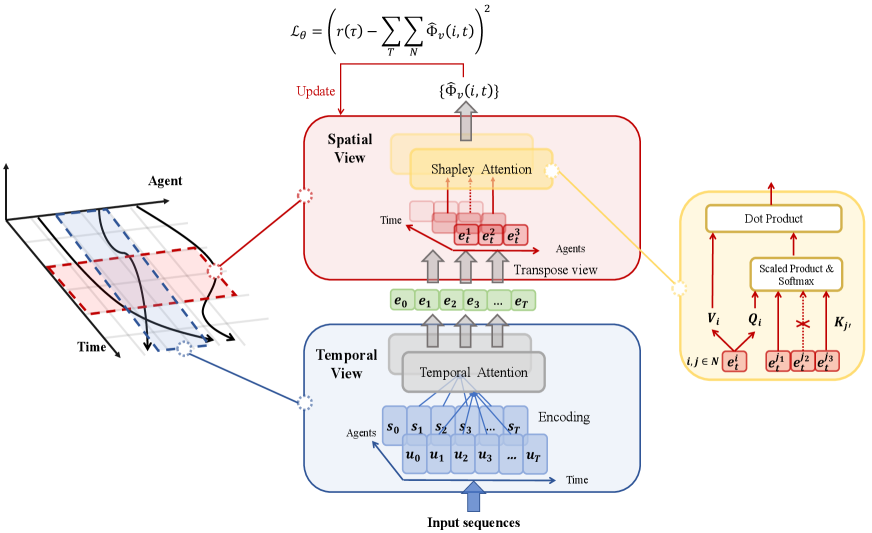
Following Eq. (3), we assume that the sum of dense global rewards along the episode can reconstruct the final return given at the last time step. Similarly, the global reward equates to the sum of all distributed individual rewards.
| (4) |
where is the distributed reward for each agent. As mentioned previously, the use of Shapley Value in cooperative games has proven beneficial, distributing the payoff of each agent and leading to faster convergence rates. Consequently, we calculate the Shapley value as the actual distributed reward for each agent.
Spatial Decomposition: Shapley Value
As indicated in (2), the Shapley Value of agent at time is computed by iterating through all possible subsets of the grand coalition:
| (5) |
where represents subsets that exclude agent , and is the marginal contribution of agent for a coalition at time :
| (6) |
where and .
Marginal Contribution Approximation In practice, it is difficult and unstable to either learn a global value function for each time step or a local value function for arbitrary coalition. When the number of agents increases, the computational complexity grows exponentially. Therefore, we propose a simple method to approximate the marginal contribution. Suppose all agents take actions sequentially to join a grand coalition . Then we define a function to estimate marginal contribution as:
where , , is an ordered coalition that agent is about to join and is the parameters of the function. It is easy to extend the above definition to the game where agents take actions simultaneously, by taking expectation over all possible permutations of coalition . In practice, we use self-attention (Shaw, Uszkoreit, and Vaswani 2018) to implement such marginal contribution approximation. The query vector for agent at time step is denoted as , where represents the encoding of the state and action of agent at time step , and is a trainable query projection matrix. Similarly, the key and value vectors for agent at time are denoted as and , respectively. The self-attention weight can be computed as follows:
| (7) |
where represents the dimension of the and . The attention weight can be interpreted as a correlation between agent and at time . When viewed from the perspective of agent , signifies that agent is not in the coalition that agent is preparing to join. Thus, a straightforward mask on other agents is sufficient to model the process of agent joining arbitrary coalition :
| (8) |
After masking irrelevant agents, the masked attention function in a matrix form:
| (9) |
where is a Hadamard product. And it is reasonable to represent the approximation of the marginal contribution of agent , i.e., . We believe that such modeling can maintain the property of exact marginal contribution.
Shapley Value Approximation As the number of agents in a multi-agent system grows, computing the exact Shapley Value for each agent becomes increasingly difficult, even when using marginal contribution approximation. To address this challenge, recent studies (Ghorbani and Zou 2019; Maleki et al. 2013) have proposed approximate methods as an alternative to the exact computation of Shapley Value. These approximation methods allow for more efficient estimation of the Shapley Value, while still capturing the essential information about each agent’s contribution to the team’s performance. To mitigate the unacceptable computational burden brought by traversing all possible coalitions, we also adopt Monte Carlo estimation for Shapley Value approximation:
| (10) |
Although other estimation methods are available (Zhou et al. 2023), for the sake of simplicity and the absence of prior knowledge, we deem Monte Carlo estimation to be both necessary and sufficient for spatial reward decomposition.
Temporal Decomposition
Due to the efficiency property of the Shapley Value, the sum of all distributed payoffs equals the value of grand coalition. Therefore, we can get the estimated global reward at time from the Shapley Value approximation of each agent, and the estimated final return can be written as:
| (11) |
In fact, the marginal contribution of an agent is seldom independent across time unless the relevant information from previous states has already been considered. To decompose the episodic return into a Markovian proxy reward function, the relations between actions and state transitions along trajectories must be established.
In practice, sequential modeling methods like Long short-term memory (LSTM) (Sak, Senior, and Beaufays 2014) or Transformer (Vaswani et al. 2017) are favored to encode the trajectory. Similar to Eq. (9), we adopt an attention function with causality masks on the state-action encoding to incorporate temporal information. Specifically, we have
| (12) |
where the query matrix is obtained by applying the trainable matrix to the output of a feed-forward layer that encodes raw state and action embeddings. Similarly, the key and value matrices are generated by the trainable matrices and , respectively. The self-attention weight is calculated using a softmax function applied to the scaled dot product of the query and key matrices, with the scaling factor and the causality mask . is a causality mask with its first -th entries equal to , and remaining entries . It ensures that at each time step , the model only attends to the states and actions before .
Overall objective
With the estimated return from Eq. (11), we can train the return decomposition model by the following objective:
| (13) |
where is the approximation of the Shapley Value of agent at time , denotes the trajectories collected in the experience buffer and denotes the parameter of the return decomposition model. The details of the training algorithm are shown in algorithm 1.
Policy optimization For every policy, the complete trajectory’s global states and actions can be fed into the return decomposition model to derive rewards for each agent at each time step, denoted as . Subsequently, the policy can be updated using algorithms like PPO (Schulman et al. 2017) or SAC (Haarnoja et al. 2018).
Experiments
In this section, we conduct experiments to evaluate the performance and effectiveness of our proposed method on the challenging problem of spatial-temporal return decomposition. We evaluate our approach using two different implementations and test it on three different environments: a newly designed environment “Alice & Bob”, as well as the cooperative navigation and predator-prey scenarios in the general multi-agent benchmark MPE (Lowe et al. 2017). The source code is available at https://github.com/zowiezhang/STAS.
Evaluate Algorithms
We compared our method with other several baseline algorithms in a scenario where rewards are given only at the game’s end. Agents receive a reward at each step and the sum of all rewards, i.e., the episodic return, after the game ends. We have evaluated two implementations of our method:
-
•
STAS (ours) denotes the default implementation of our algorithm. First, we input the state-action sequence into a temporal attention module, which is designed to extract essential information from previous states. Next, we use a Shapley attention module to approximate the Shapley value for each agent. The predicted Shapley value is a measure of an agent’s instant contribution to the team’s final performance.
-
•
STAS-ML (ours) is our alternative implementation, where “ML” stands for multi-layers. We organize temporal and spatial components into layers, each comprising a single temporal attention module and a single Shapley attention module. By stacking multiple layers, we construct our final prediction of the Shapley value. Each layer captures increasingly complex dependencies and interactions among agents, resulting in more accurate estimates of their individual contributions.
We compare with several existing baselines under the same settings, including QMIX (Rashid et al. 2020), COMA (Foerster et al. 2018) and SQDDPG (Wang et al. 2020a)
The specific implementation of our methods We utilize a temporal attention module to extract crucial information from previous states. To ensure causality, each state only receives information from earlier states through a causality mask. Positional embedding is employed to capture the relative positions of each state in the sequence. The Shapley attention module processes the learned embeddings for each agent to estimate their Shapley value. Our policy model is based on independent PPO (Schulman et al. 2017).

Extreme delayed reward environment
In this experiment section, we designed a toy example environment called “Alice & Bob” to verify the effectiveness of our method in an extremely delayed reward setting, as illustrated in Fig 2. In this task, agents Alice and Bob, unable to communicate, must collaboratively secure a treasure within a set number of steps, following a specific order and relying solely on their individual environmental states. They must adapt to the cooperative pattern dictated by the environment. The task’s complexity is heightened by an extremely delayed reward system, where rewards accumulate and are only dispensed upon task completion, posing a substantial challenge to solving methods.
Environment settings
At the beginning of the task, both Alice and Bob are locked in a room, but Alice can use the key in her room to unlock Bob’s room. Once the key is touched, the door of Bob’s room will be opened. Then Bob can get out of the room and find the key to Alice’s room. After both of them get out of the room, they can go and get the treasure. The reward setting is that if any of them hit the wall when exploring, they will get a minus reward -0.2; if at the end of the game, they reach the treasure, they will get an extra reward of 200 and finish the task, and if they still not get the treasure within the maximum step, they will get the reward sum of each step as the whole return to force stop the task. Each agent has 4 different actions, namely, move_up, move_down, move_left and move_right.
Results


| COMA | QMIX | SQDDPG | STAS | |
|---|---|---|---|---|
| Coefficient | ||||
| Two-tailed -value | 0.9218 |
As presented in Fig 3, our methods STAS and STAS-ML outperform baselines, with STAS soaring to an average reward of 200 and a treasure rate of 0.9 at 30k episodes. QMIX improves slightly at 10k episodes but then declines. SQDDPG improves after 60k episodes, reaching an average reward of 130 and a treasure rate of 0.65. COMA is ineffective, with minimal rewards and a treasure rate of 0. The variance of QMIX and SQDDPG is high throughout training. Our results demonstrate our method’s effectiveness in a challenging, extremely delayed reward environment, successfully learning cooperation patterns.
Multi-agent Particle Environment
Environment settings
We selected two scenarios from MPE, namely cooperative navigation and predator-prey, to evaluate the performance of all algorithms. In task cooperative navigation, agents are asked to reach landmarks. Agents are rewarded based on how far any agent is from each landmark and penalized if they collide with other agents. In task predator-prey, agents cooperate to catch preys. Agents are rewarded when any of them catch the prey and penalized if they stay away from the preys. All preys are controlled by a pre-trained policy. In our settings, rewards are only revealed at the end of each episode.
Results
The results in Fig 4 demonstrate our approach’s superior performance and sample efficiency over all baselines, particularly in environments with delayed rewards. Baselines show increased variance and ineffectiveness as agent numbers rise, likely due to the complexity in assessing individual agent contributions in larger cooperative systems without mid-term global rewards. While STAS-ML surpasses STAS in the predator-prey task with three agents, it shows comparable results in other tasks. This implies that forgoing Shapley Value properties may reduce performance in complex scenarios but enhance sample efficiency in simpler, smaller-agent tasks.
Ablations
We conducted several ablation experiments to evaluate different components of the STAS. Fig 5(a) demonstrates the impact of different practical methods of the spatial transformer. It shows that when the sample number of Shapley value approximation is 1, not only is the performance the worst but the variance is also larger, making it less stable. When the sample number is 5, the performance is optimal, as increasing the sample number leads to a more accurate estimation of the true value. However, when the sample number is 3, the performance is already close to that of 5, indicating that the performance is good enough with 3 samples.
Fig 5(b) demonstrates the impact of using different numbers of layers in the STAS-ML. When the number of layers is 1, the performance shows higher variance and is less stable. This may be because a single layer is not sufficient to extract high-level hidden information. As the number of layers increases, the performance significantly improves. When the number of layers is 3 and 5, the performance is already very close, indicating that the model is able to extract the relevant information about the interactions between the agents with several layers.
Following Wang et al. (2020a), we conducted an experiment to verify the effectiveness of the Shapley value. We computed the Pearson coefficient correlating the credits assigned to each agent with the inverse of their distance to the prey in a predator-prey scenario involving three agents. Table 1 indicates that our approach surpasses all baseline methods in fairness. Moreover, SQDDPG demonstrates considerable effectiveness. These results robustly confirm our rationale for integrating Shapley value to effectively address credit assignment challenges.
Conclusion
In this paper, we focus on the credit assignment problem in multi-agent learning with delayed episodic return. We introduce return decomposition methods to this problem, and we propose an novel approach called STAS. Our approach utilizes the Shapley value to evaluate each agent’s contribution and combines these contributions on both spatial and temporal scales to fit with the real episodic return from the environment. Our experimental results demonstrate that STAS outperforms all baselines, showing lower variance and faster convergence speed. In future work, we plan to include more baselines while extending it to more challenging tasks.
Acknowledgments
This work is sponsored by National Natural Science Foundation of China (62376013), Collective Intelligence & Collaboration Laboratory (Open Fund Project No. QXZ23014101)
References
- Arjona-Medina et al. (2019) Arjona-Medina, J. A.; Gillhofer, M.; Widrich, M.; Unterthiner, T.; Brandstetter, J.; and Hochreiter, S. 2019. RUDDER: Return Decomposition for Delayed Rewards. In NeurIPS 32, 13544–13555.
- Bilbao and Edelman (2000) Bilbao, J. M.; and Edelman, P. H. 2000. The Shapley value on convex geometries. Discrete Applied Mathematics, 103(1-3): 33–40.
- Busoniu, Babuska, and De Schutter (2008) Busoniu, L.; Babuska, R.; and De Schutter, B. 2008. A Comprehensive Survey of Multiagent Reinforcement Learning. IEEE Transactions on Systems, Man, and Cybernetics, Part C (Applications and Reviews), 38(2): 156–172.
- Du et al. (2019) Du, Y.; Han, L.; Fang, M.; Dai, T.; Liu, J.; and Tao, D. 2019. LIIR: learning individual intrinsic reward in multi-agent reinforcement learning. In Proceedings of the 33rd International Conference on Neural Information Processing Systems (NeurIPS), 4403–4414.
- Du et al. (2023) Du, Y.; Leibo, J. Z.; Islam, U.; Willis, R.; and Sunehag, P. 2023. A Review of Cooperation in Multi-agent Learning. arXiv preprint arXiv:2312.05162.
- Foerster et al. (2018) Foerster, J. N.; Farquhar, G.; Afouras, T.; Nardelli, N.; and Whiteson, S. 2018. Counterfactual Multi-Agent Policy Gradients. In AAAI 2018, 2974–2982.
- Gangwani, Zhou, and Peng (2020) Gangwani, T.; Zhou, Y.; and Peng, J. 2020. Learning Guidance Rewards with Trajectory-space Smoothing. In NeurIPS 33.
- Ghorbani and Zou (2019) Ghorbani, A.; and Zou, J. 2019. Data shapley: Equitable valuation of data for machine learning. In International Conference on Machine Learning, 2242–2251. PMLR.
- Haarnoja et al. (2018) Haarnoja, T.; Zhou, A.; Hartikainen, K.; Tucker, G.; Ha, S.; Tan, J.; Kumar, V.; Zhu, H.; Gupta, A.; Abbeel, P.; et al. 2018. Soft actor-critic algorithms and applications. arXiv preprint arXiv:1812.05905.
- Han et al. (2022) Han, B.; Ren, Z.; Wu, Z.; Zhou, Y.; and Peng, J. 2022. Off-Policy Reinforcement Learning with Delayed Rewards. In ICML 2022, volume 162, 8280–8303.
- Li et al. (2021) Li, J.; Kuang, K.; Wang, B.; Liu, F.; Chen, L.; Wu, F.; and Xiao, J. 2021. Shapley Counterfactual Credits for Multi-Agent Reinforcement Learning. In KDD 2021, 934–942.
- Liu et al. (2019a) Liu, Y.; Luo, Y.; Zhong, Y.; Chen, X.; Liu, Q.; and Peng, J. 2019a. Sequence Modeling of Temporal Credit Assignment for Episodic Reinforcement Learning. CoRR, abs/1905.13420.
- Liu et al. (2019b) Liu, Y.; Luo, Y.; Zhong, Y.; Chen, X.; Liu, Q.; and Peng, J. 2019b. Sequence modeling of temporal credit assignment for episodic reinforcement learning. arXiv preprint arXiv:1905.13420.
- Lowe et al. (2017) Lowe, R.; Wu, Y.; Tamar, A.; Harb, J.; Abbeel, P.; and Mordatch, I. 2017. Multi-Agent Actor-Critic for Mixed Cooperative-Competitive Environments. NeurIPS 30.
- Maleki et al. (2013) Maleki, S.; Tran-Thanh, L.; Hines, G.; Rahwan, T.; and Rogers, A. 2013. Bounding the estimation error of sampling-based Shapley value approximation. arXiv preprint arXiv:1306.4265.
- Ng, Harada, and Russell (1999) Ng, A. Y.; Harada, D.; and Russell, S. 1999. Theory and application to reward shaping. In Proceedings of the Sixteenth International Conference on Machine Learning.
- Panait and Luke (2005) Panait, L.; and Luke, S. 2005. Cooperative multi-agent learning: The state of the art. Autonomous agents and multi-agent systems, 11: 387–434.
- Patil et al. (2022) Patil, V. P.; Hofmarcher, M.; Dinu, M.; Dorfer, M.; Blies, P. M.; Brandstetter, J.; Arjona-Medina, J. A.; and Hochreiter, S. 2022. Align-RUDDER: Learning From Few Demonstrations by Reward Redistribution. In ICML 2022, volume 162, 17531–17572.
- Perrusquía, Yu, and Li (2021) Perrusquía, A.; Yu, W.; and Li, X. 2021. Multi-agent reinforcement learning for redundant robot control in task-space. International Journal of Machine Learning and Cybernetics, 12: 231–241.
- Rashid et al. (2020) Rashid, T.; Farquhar, G.; Peng, B.; and Whiteson, S. 2020. Weighted QMIX: Expanding Monotonic Value Function Factorisation for Deep Multi-Agent Reinforcement Learning. In NeurIPS 33.
- Ren et al. (2022) Ren, Z.; Guo, R.; Zhou, Y.; and Peng, J. 2022. Learning Long-Term Reward Redistribution via Randomized Return Decomposition. In ICLR 2022.
- Sak, Senior, and Beaufays (2014) Sak, H.; Senior, A. W.; and Beaufays, F. 2014. Long short-term memory recurrent neural network architectures for large scale acoustic modeling.
- Schulman et al. (2017) Schulman, J.; Wolski, F.; Dhariwal, P.; Radford, A.; and Klimov, O. 2017. Proximal policy optimization algorithms. arXiv preprint arXiv:1707.06347.
- Shapley (1997) Shapley, L. S. 1997. A value for n-person games. Classics in game theory, 69.
- Shaw, Uszkoreit, and Vaswani (2018) Shaw, P.; Uszkoreit, J.; and Vaswani, A. 2018. Self-attention with relative position representations. arXiv preprint arXiv:1803.02155.
- She, Gupta, and Kochenderfer (2022) She, J.; Gupta, J. K.; and Kochenderfer, M. J. 2022. Agent-time attention for sparse rewards multi-agent reinforcement learning. arXiv preprint arXiv:2210.17540.
- Son et al. (2019) Son, K.; Kim, D.; Kang, W. J.; Hostallero, D.; and Yi, Y. 2019. QTRAN: Learning to Factorize with Transformation for Cooperative Multi-Agent Reinforcement Learning. In ICML 2019, volume 97, 5887–5896.
- Sundararajan and Najmi (2020) Sundararajan, M.; and Najmi, A. 2020. The many Shapley values for model explanation. In International conference on machine learning, 9269–9278. PMLR.
- Sunehag et al. (2018) Sunehag, P.; Lever, G.; Gruslys, A.; Czarnecki, W. M.; Zambaldi, V. F.; Jaderberg, M.; Lanctot, M.; Sonnerat, N.; Leibo, J. Z.; Tuyls, K.; and Graepel, T. 2018. Value-Decomposition Networks For Cooperative Multi-Agent Learning Based On Team Reward. In AAMAS 2018, 2085–2087.
- Vaswani et al. (2017) Vaswani, A.; Shazeer, N.; Parmar, N.; Uszkoreit, J.; Jones, L.; Gomez, A. N.; Kaiser, Ł.; and Polosukhin, I. 2017. Attention is all you need. Advances in neural information processing systems, 30.
- Vinyals et al. (2019) Vinyals, O.; Babuschkin, I.; Czarnecki, W. M.; Mathieu, M.; Dudzik, A.; Chung, J.; Choi, D. H.; Powell, R.; Ewalds, T.; Georgiev, P.; et al. 2019. Grandmaster level in StarCraft II using multi-agent reinforcement learning. Nature, 575(7782): 350–354.
- Wang et al. (2020a) Wang, J.; Zhang, Y.; Kim, T.; and Gu, Y. 2020a. Shapley Q-Value: A Local Reward Approach to Solve Global Reward Games. In AAAI 2020, 7285–7292.
- Wang et al. (2020b) Wang, T.; Dong, H.; Lesser, V. R.; and Zhang, C. 2020b. ROMA: Multi-Agent Reinforcement Learning with Emergent Roles. In ICML 2020, volume 119, 9876–9886.
- Wang et al. (2021) Wang, Y.; Han, B.; Wang, T.; Dong, H.; and Zhang, C. 2021. DOP: Off-Policy Multi-Agent Decomposed Policy Gradients. In ICLR 2021.
- Xiao, Ramasubramanian, and Poovendran (2022) Xiao, B.; Ramasubramanian, B.; and Poovendran, R. 2022. Agent-Temporal Attention for Reward Redistribution in Episodic Multi-Agent Reinforcement Learning. In AAMAS 2022, 1391–1399.
- Yang et al. (2020) Yang, Y.; Hao, J.; Liao, B.; Shao, K.; Chen, G.; Liu, W.; and Tang, H. 2020. Qatten: A General Framework for Cooperative Multiagent Reinforcement Learning. CoRR, abs/2002.03939.
- Zhang et al. (2023) Zhang, Y.; Du, Y.; Huang, B.; Wang, Z.; Wang, J.; Fang, M.; and Pechenizkiy, M. 2023. Interpretable Reward Redistribution in Reinforcement Learning: A Causal Approach. In Thirty-seventh Conference on Neural Information Processing Systems.
- Zhou et al. (2023) Zhou, Z.; Xu, X.; Sim, R. H. L.; Foo, C. S.; and Low, B. K. H. 2023. Probably approximate Shapley fairness with applications in machine learning. In Proceedings of the AAAI Conference on Artificial Intelligence, volume 37, 5910–5918.