Stabilizing Linear Passive-Aggressive Online Learning with Weighted Reservoir Sampling
Abstract
Online learning methods, like the seminal Passive-Aggressive (PA) classifier, are still highly effective for high-dimensional streaming data, out-of-core processing, and other throughput-sensitive applications. Many such algorithms rely on fast adaptation to individual errors as a key to their convergence. While such algorithms enjoy low theoretical regret, in real-world deployment they can be sensitive to individual outliers that cause the algorithm to over-correct. When such outliers occur at the end of the data stream, this can cause the final solution to have unexpectedly low accuracy. We design a weighted reservoir sampling (WRS) approach to obtain a stable ensemble model from the sequence of solutions without requiring additional passes over the data, hold-out sets, or a growing amount of memory. Our key insight is that good solutions tend to be error-free for more iterations than bad solutions, and thus, the number of passive rounds provides an estimate of a solution’s relative quality. Our reservoir thus contains previous intermediate weight vectors with high survival times. We demonstrate our WRS approach on the Passive-Aggressive Classifier (PAC) and First-Order Sparse Online Learning (FSOL), where our method consistently and significantly outperforms the unmodified approach. We show that the risk of the ensemble classifier is bounded with respect to the regret of the underlying online learning method.
1 Introduction
Online learning algorithms are especially attractive when working with high-volume and high-dimensional streaming data, out-of-core processing, and other throughput-sensitive applications [1]. For example, the seminal Vowpal Wabbit uses importance-weighted online learning algorithms [2] to reach high quality solutions quickly, with an optional second pass using LBFGS to refine the solution. The MOA library still uses the Pegasos algorithm as its linear classifier [3]. Most relevantly, online learning algorithms are particularly appealing for binary classification tasks, such as web spam classification [1]. Such algorithms often enjoy fast theoretical convergence rates due to their fast adaptation to errors on individual data points, as opposed to batch or offline learning.
However, in real-world deployment, online algorithms can be very sensitive to noisy observations in the data stream and over-correct, resulting in out-of-sample performance dropping precipitously between timesteps. Indeed, in many cases (see Figure 1), an online learning algorithm might achieve over test accuracy after a given timestep, but then see its test accuracy drop by after over-correcting on the next observation in the data stream. In many real-world settings, it may be infeasible computationally or memory-wise to maintain a hold-out evaluation set to select the highest-performance solutions learned by our online algorithm. It may also be practically infeasible to train our classifier over multiple passes of a given dataset or when online algorithms are used for “any-time” ready predictions.
In this paper, we introduce a weighted reservoir sampling (WRS) [4] based approach that dramatically mitigates the aforementioned accuracy fluctuations. Our proposed method, WRS-Augmented Training (WAT), neither requires a hold-out evaluation set nor additional passes over the training data. Most importantly, WAT can be used to stabilize any passive-aggressive online learning algorithm. We demonstrate the promise of our WAT method on the Passive Aggressive Classifier (PAC) [5] and First-Order Sparse Online Learning (FSOL) [1] methods — creating two new methods PAC-WRS and FSOL-WRS. Strikingly, across 16 benchmark datasets, WAT is able to mitigate test accuracy fluctuations in all 16 datasets on FSOL and 14 datasets on PAC. To analyze the theoretical effectiveness of our method, we situate our approach in the online-to-batch conversion literature, enabling us to obtain generalization bounds on i.i.d. data streams.

2 Review of related work
Our work is motivated in part by a real-world need in malware detection [6], in which large datasets make online methods particularly attractive [7, 8], and a naturally noisy labeling process inhibits standard passive-aggressive methods [9, 10, 11, 12]. We show results for the EMBER malware benchmark in Appendix C.
Online learning. In online learning for linear binary classification, one maintains a solution vector , where is the dimensionality of our data points (usually quite large), and represents the timestep. At each timestep , we observe a single observation from a high-throughput data stream, with feature vector and class label . Given , an online learning algorithm will make a minor (potentially no effect) update to to output , before receiving the next in the data stream. The classification rule using on any test point is simply . The goal is that as , the sequence of will enjoy low cumulative loss. Towards this end, many online learning algorithms with various update rules have been proposed in the literature, including the Passive-Aggressive Classifier (PAC) [5], the Adaptive Regularization of Weight Vectors (AROW) methods [13] and the Adaptive Subgradient method (ADAGRAD) [14]. Some online learning algorithms have also been designed to specifically learn sparse solutions for (proportion of zero entries), such as Truncated Gradient method [15], Stochastic MIrror Descent Algorithm made Sparse method (SMIDAS) [16], Regularized Dual Averaging (RDA) method [17], and First-Order and Second-Order Sparse Online Learning methods (FSOL and SSOL) [1]. In general, these sparsity-inducing methods are powered by some combination of solution truncation and L1 norm minimization.
Passive-aggressive online learning. Within the family of online learning algorithms, a passive-aggressive algorithm is one whose update rule makes no update to if is classified correctly with sufficient margin. That is, we passively leave . If a margin error occurs, we aggressively update such that the error is fully correct (though a regularization penalty will tamper the degree of aggressiveness). Usually, correct classification with sufficient margin is defined using the hinge loss — the algorithm remains passive at timestep if Next, we introduce the two passive-aggressive algorithms that we will use to test our WRS-Augmented Training method.
Passive-Aggressive Classifier (PAC). Introduced by Crammer et al., PAC is actually a family of three algorithms: PA, PA-I, and PA-II [5]. The base PA algorithm update rule seeks to solve the following constrained optimization problem:
Because of the hard constraint of forcing to satisfy , the optimization is particularly vulnerable to noisy data. As such, Crammer et al. introduce a new constrained optimization function with a slackness hyperparameter to allow for some residual hinge loss and induce less aggressive, but presumably more stable updates:
where setting corresponds to PA-I and to PA-II. From initial testing, PA-I and PA-II performed very similarly, with a slight edge to PA-II. As such, for this paper, we will focus on PA-II, which performs the following closed-form update when in aggressive mode [5]: For the remainder of this paper, “PAC" will refer to PA-II.
First-Order Sparse Online Learning (FSOL). Introduced by Zhao et al. [1], FSOL is a passive-aggressive algorithm which attempts to find sparse solutions for . Governed by a learning rate and a sparsity parameter , FSOL keeps track of two vectors and performs the following update rules when in aggressive mode [1]:
where and takes the maximum of each element in and . Zhao et al. note that the above update rules are identical to that of Xiao’s RDA method with soft -norm regularization [17, 1].
Weighted Reservoir Sampling (WRS). Suppose we have a collection of items , with corresponding nonnegative weights . Our goal is to collect a size- weighted random sample from in one pass (imagine this process is indexed by time), where the population size is potentially unknown. Introduced by Efraimidis and Spirakis [4], weighted random sampling with a reservoir, which we shorten to weighted reservoir sampling (WRS), is an algorithm that allows us to collect such a size- weighted random sample under the aforementioned conditions. Specifically, as we are making our one pass through the items in , at each timestep , we maintain and update a reservoir — a temporary storage unit with a maximum capacity of items, with each item in the reservoir a potential candidate for our final size- sample. At time , the items that are currently in the reservoir will constitute our sample of size-. We invite the interested reader to look at Algorithm A in [4] for specific details.
Online-to-batch conversion. Online learning algorithms such as PAC generally do not impose any restrictions on the distribution of the training data sequence. Their regret bounds aim to control the cumulative loss of the algorithm over any sequence of data, compared with a minimal-loss fixed model : . When using a fixed model to classify unseen data, we need to impose an i.i.d. assumption on the data stream in order to measure the risk, or expected generalization error, of the model. Note that the distribution itself is arbitrary and can still permit outliers or mixtures. Then the population risk is defined as .
To theoretically describe our algorithm, we leverage work on online-to-batch conversion, which takes an online algorithm with known regret bounds on an i.i.d. sequence of data and extracts a stable final model with low risk. For example, in the online perceptron algorithm, earlier work studied the pocket approach, which selects the longest-surviving model in the sequence as the final model [18, 19]. Other well-known approaches use the uniform average of the whole model sequence or the best-performing model over a validation set [20].
As will be seen, our method generalizes these approaches to utilize multiple long-survival models as an ensemble model. Furthermore, we will introduce novel improvements, including a limited-size reservoir with probabilistic sampling. The risk bounds for our WAT model leverage improved techniques from [21, 22]. Our experimental results also demonstrate that our novel conversion technique outperforms prior baselines (see Appendix D).
3 Our method: WRS-Augmented Training (WAT)
In one extreme, if a candidate solution from a passive-aggressive algorithm had perfect classification with sufficient margin on any given data point, then the subsequent number of passive steps taken after time (i.e., number of timesteps that our algorithm is in passive mode before going aggressive again) would be infinite. In the other extreme, if a candidate solution had extremely low performance, then our passive-aggressive algorithm is likely to go aggressive very soon after time , implying a very small subsequent number of passive steps after time . In short, our key insight is that high-performing solutions tend to be error-free for more iterations than low-performing solutions. As such, the subsequent number of passive steps taken after the formation of provides an estimate of ’s relative quality (i.e., test accuracy).
However, we do not want to take the intermediate solution that had the most passive updates as this, too, can be noise (and luck) sensitive. Ideally, we would like to sample from the merging distribution of as they occur, and take an average of those solutions to obtain a singular, highly robust, solution vector that performs well with little variance. But, we do not wish to store all due to intractability.
Putting these thoughts together, our WRS-Augmented Training (WAT) method functions as follows. Given a base passive-aggressive algorithm (e.g., PAC or FSOL), we will run said algorithm through our data stream , as normal, but keep a size- reservoir of promising candidate solutions. The reservoir approach allows us to run through our data stream and collect a weighted random sample of candidate solutions of size-, weighted by their subsequent number of passive steps and without storing all intermediate solutions.
Naturally, this setup is suited for Efraimidis and Spirakis’s WRS algorithm. Procedurally, every timestep that our algorithm goes aggressive, we obtain a new active candidate solution. Right before we apply our aggressive mode update rule, we will add the outgoing candidate solution to our size- reservoir (and remove a current resident of the reservoir, if necessary) following the steps of the WRS algorithm. At any timestep , we can form an ensemble solution by taking an average of the candidate solutions currently in our reservoir. Hopefully, at any timestep , will have more stable test performance than the current active candidate solution .
3.1 WAT variants
We will experiment with a few additional variants of the WAT method. First, instead of weighting using the subsequent number of passive steps (which we denote as standard weights), what if we weight using the exponentiated subsequent number of passive steps (which we denote as exponential weights)? The idea with exponential weights is that it is closer in practice to deterministically picking the candidate solutions with the largest number of subsequent passive steps, while still maintaining some stochasticity — i.e., a “greedier" policy. Second, when constructing our ensemble solution , should we take a simple average of the residents in our reservoir or a weighted average? Third, there are reasonable concerns that constructing via averaging might negate the sparsity advantages of a method like FSOL, due to different candidates in the reservoir containing s in different entries. However, if the majority of candidate solutions in the reservoir contain s at a given entry, what if we tried zeroing out said entry in , as it is likely to be uninformative? We denote this add-on as voting-based zeroing.
We present the WAT method in full detail in Algorithm 1. To clarify, the elements in the data structures , , and (all of which are size- arrays) are paired with each other, so that when we add/remove an element in , the corresponding elements in and are removed as well. To be fully clear, contains candidate solution vectors , with each . The vector contains scalar values , and likewise for the vector .
3.2 Theoretical Analysis
One of the goals of our method is to choose a set of effective models as the algorithm runs live, without the need for expensive evaluation on a validation set. In this section we first provide validity arguments for using observed survival as a proxy to select high-accuracy models. These are finite-sample bounds based on reasoning about the reservoir . Note that we are interested in studying generalization to unseen data, a complementary setting to prior work which shows convergence in terms of training set error for the perceptron model [19]. After establishing validity, we will turn to learning bounds for our ensemble model risk in the i.i.d. setting. Proofs are deferred to Appendix A.
Validity analysis. We assume a given dataset is an i.i.d. sequence sampled from a generating distribution . We first suppose that is the 0-1 loss, that is . Then the risk is the probability that a random is misclassified by . At any time , we have an online model , for which we define the survival time to be the number of subsequent correct classifications, stopping when misclassifies a sample. As does not change until an error occurs, at any finite time we only collect updated models into .
Our first result bounds the difference in risk among two models in : (1) the minimal-risk hypothesis which we do not know, and (2) the longest-surviving hypothesis which we observe. We also denote and to be their respective survival times.
Theorem 1.
Let be the updated outputs of an online PA algorithm on inputs . Also define as the minimal achievable risk of any model, such that almost surely. Then
This immediately leads to
Corollary 1.
With prob. , .
While this bound explains the use of top-1 survival in the worst case, we further justify the use of an ensemble (or reservoir) of top-surviving models. Specifically, given the use of top- models, there is always a certain probability that the top- can lower the risk. Since is a base case, this implies that any value of is worthy of consideration, until this probability decays to 0.
To simplify the notation, we sort the models in by decreasing survival time , with corresponding re-indexed weights and risks . We also add an assumption, that there is a partition of such that and , and that . That is, there is a set of good and bad models in terms of risk. In the Appendix we show that the assumption is readily satisfied.
Theorem 2.
Let be the averaged risk of the top- surviving models, and let be the averaged risk including the next highest survival model. Then with probability at least .
Finally note that we can define an averaged model (weighted or unweighted) . For any convex with risk , such as the hinge loss, Jensen’s inequality gives .
Learning bounds. Now we turn to generalization bounds of our method, when run to a fixed stopping time . We assume more generally that is convex, such as the hinge loss. Furthermore we suppose that the loss of any point in the training set is bounded by . This is a safe assumption for many passive-aggressive algorithms, where the input data is normalized and the update steps are not too large.
Theorem 3.
Suppose is convex and bounded from above by . By time , suppose the reservoir contains models, with survival time of each at least . Let be the cumulative loss of the WAT reservoir sequence, with formally defined in the proof. Then w.p. ,
The result shows that the risk of the ensemble model is stochastically bounded by the cumulative loss of the online procedure. By applying known regret bounds for the underlying online algorithms (e.g. PAC or FSOL), we can further bound the risk in terms of the original learner, and subsequently the optimal risk. In particular, we can “abstract out” the actual online learning method in the proof, as a generic regret bound of form , for any . Depending on the algorithm often or even .
With this in hand, we can show that the risk actually approaches the minimal risk. One additional assumption is required: (the WRS sequence has lower cumulative loss than the original learner). By definition, the reservoir contains the models which have longest survivals, and hence lowest regret density. So this statement is readily satisfied, as long as the distributions of non-zero losses are not different among the two sequences. In fact, under certain conditions, the inequality is likely strict which further improves the bound. Altogether we obtain:
Theorem 4.
Given a PA algorithm, let be its cumulative loss, and be the algorithm-specific excess regret. Then with probability , the deviation in risk of our WRS model from the optimal model is bounded as
Dataset Sparsity Avazu (App) [23] (via LIBSVM) 1000000 14596137 10217295 4378842 0.999985 Avazu (Site) [23] (via LIBSVM) 1000000 25832830 18082981 7749849 0.999985 Criteo (via LIBSVM) 1000000 51882752 36317926 15564826 0.999961 Dexter [24] 20000 600 420 180 0.995319 Dorothea [25] 100000 1150 805 345 0.990909 KDD2010 (Algebra) [26] (via LIBSVM) 20216830 8918054 6242637 2675417 0.999998 MNIST8 (4+9) [27, 28] (via LIBSVM) 784 1591785 1114249 477536 0.757170 News20 [29] (via LIBSVM) 1355191 19954 13967 5987 0.999664 Newsgroups (Binary, CS) [30, 31] (via sklearn) 101631 18311 12817 5494 0.999049 PCMAC [32] 3289 1943 1360 583 0.985418 RCV1 [33] (via LIBSVM) 47236 697641 488348 209293 0.998451 Real-Sim (McCallum via LIBSVM) 20958 72201 50540 21661 0.997549 SST-2 [34] 13757 67337 47135 20202 0.999421 URL [35] (via LIBSVM) 3231961 2396130 1677291 718839 0.999964 W8A [36] (via LIBSVM) 300 59245 41471 17774 0.957585 Webspam [37] (via LIBSVM) 254 350000 244999 105001 0.664833
4 Numerical experiments
We combine WAT with base PAC and FSOL, forming two new methods PAC-WRS and FSOL-WRS111Code available at https://github.com/FutureComputing4AI/Weighted-Reservoir-Sampling-Augmented-Training. We evaluate their performances across 16 binary classification datasets listed in Table 1. Please see Appendix B for more dataset details. We are interested in three metrics: 1) Final test accuracy: proportion of test set data points correctly-classified by solution obtained after making one pass through the training data. 2) Final sparsity: proportion of zeroes in our classification solution obtained after making one pass through the training data. 3) Relative oracle performance (ROP): let be the test accuracy of our base model (either PAC or FSOL) at time and be the test accuracy of our model of interest (either base PAC, base FSOL, PAC-WRS, or FSOL-WRS). Then, define to be the cumulative maximum test accuracy of the base method at time . In other words, represents the highest performance we could obtain if we had an oracle telling us which candidate solution vector we encountered was best. Then, define . Intuitively, if a method has very stable test accuracy over time with minimal fluctuations, then ROP should be close to , or negative (i.e. achieving a higher test accuracy than the oracle). In contrast, a large, positive ROP suggests fluctuations in test accuracy.
Because we are interested in the stability of WAT’s test-set accuracy over the entirety of the training run, it is most illustrative to look at figures when possible. Representative figures will be shown in the main paper, with all figures for all datasets in the appendix. When running any algorithm (PAC, FSOL, PAC-WRS, or FSOL-WRS) on any dataset, we perform a random 70/30 train-test split. We begin by tuning the , , and hyperparameters for base PAC and FSOL, with details located in Appendix B. For PAC-WRS and FSOL-WRS, we use the hyperparameters for the corresponding base models, but try all possible WAT variants of weighting scheme (standard or exponential), averaging scheme (simple vs. weighted), voting-based zeroing (True or False), and reservoir size . We perform five trials for each PAC-WRS and FSOL-WRS variant with randomized shuffles of the training and test data, running through the training data only once for each trial. All candidate solutions are initialized as the vector. Please see more experimental details in Appendix B.
4.1 Stabilizing test performance
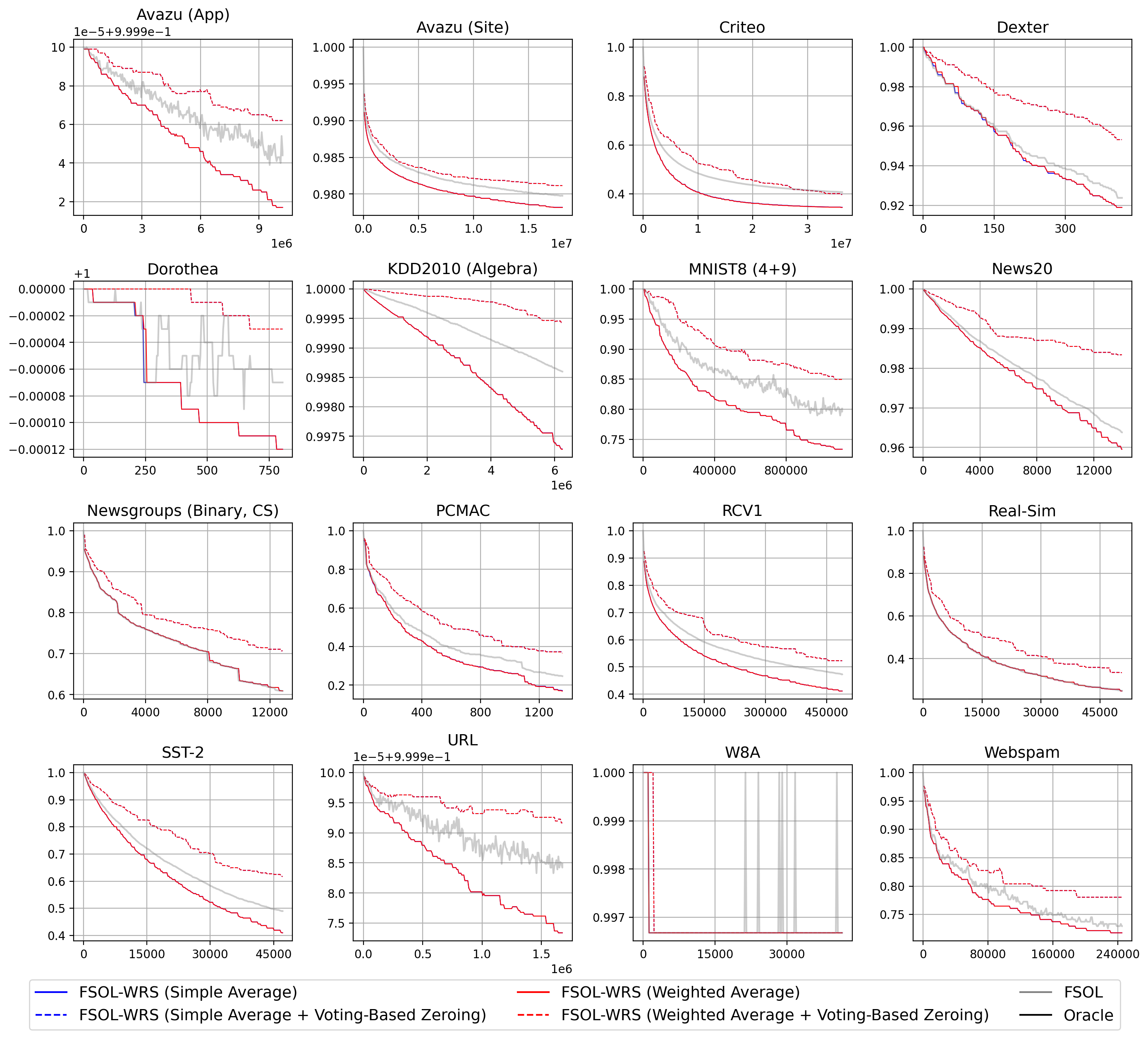
Figure 1 shows visually how PAC-WRS and FSOL-WRS are highly-effective at stabilizing base PAC and FSOL’s wildly-fluctuating test accuracy on Avazu (App) and News20. Corresponding figures for all 16 datasets and PAC-WRS/FSOL-WRS variants can be found in Appendix G.2. From Figure 2, we see that PAC-WRS is highly-effective at reducing ROP compared to base PAC, and that the larger the reservoir size , the more stable the resultant test accuracy for becomes. Furthermore, looking more carefully at MNIST8 (4+9), we observe that many PAC-WRS variants were able to achieve negative ROP values, suggesting that could achieve higher test accuracies than even the oracle. Corresponding figures for all 16 datasets can be found in Appendix G.1.

Simple Average Weighted Average Standard Exp. Standard Exponential PAC 13 14 13 11 FSOL 16 13 16 11
From Table 2, we observe that FSOL-WRS with standard weights and simple averaging successfully stabilized test accuracy in all 16 tested datasets compared to base FSOL, as measured via ROP.
PAC-WRS with exponential weights and simple averaging successfully stabilized test accuracy in 14 of 16 tested datasets compared to base PAC. Following the best practices in [38, 39], we perform Wilcoxon signed-rank tests for statistical significance on the differences in ROP between PAC/FSOL-WRS versus base PAC and FSOL, taking into account performance on all 16 datasets. At a significance level of , we find that both PAC/FSOL-WRS achieve statistically-significant reductions in ROP compared to their corresponding base models when equipped with standard weights ( in each case, see Table 6 in Appendix F).
These results also suggest that standard weights are preferable to exponential weights. This makes sense because using exponential weights may be too “greedy," causing the algorithm to overly trust in the number of passive steps as an indicator of test performance, polluting the reservoir with poor “lucky" candidate solutions, and refusing to remove them later.
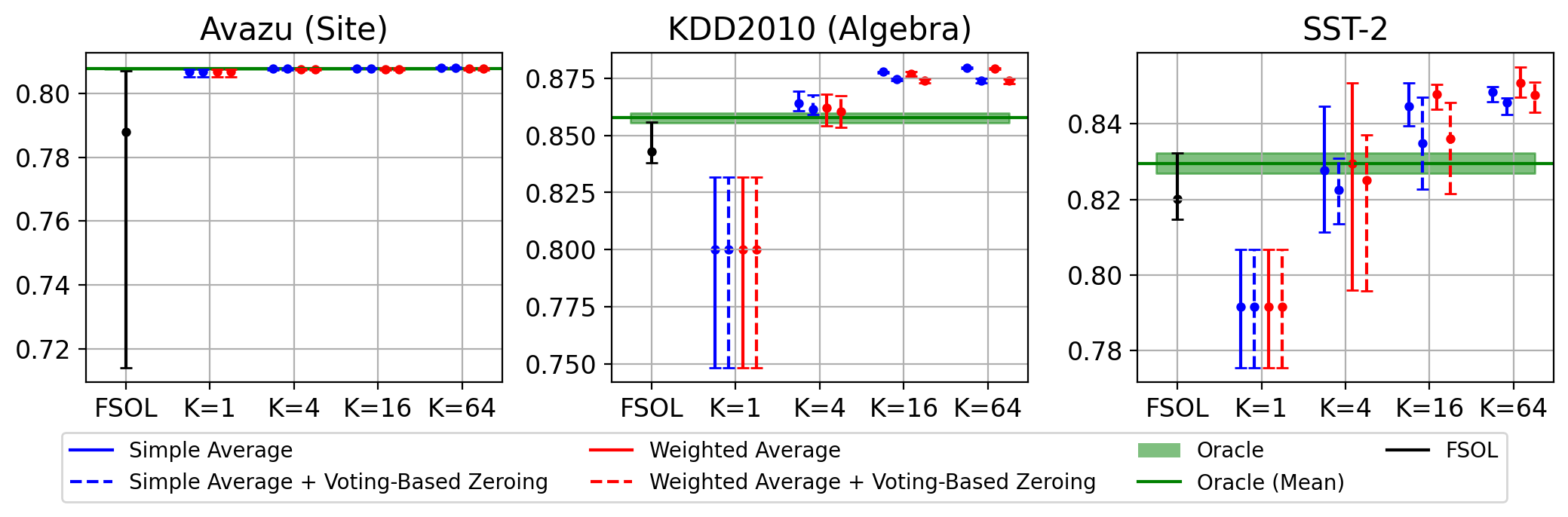
A note on final test accuracy. From Figure 3, we see that the final test accuracies achieved by FSOL-WRS are not only higher on average than base FSOL, but also have significantly lower variance. On these datasets, there is no significant difference between FSOL-WRS variants with or without voting-based zeroing. As expected, final test accuracy seems to be higher for larger values of reservoir size . However, Wilcoxon signed-rank tests to compare PAC-WRS and FSOL-WRS’s improvements in final test accuracy over base PAC and FSOL indicate that FSOL-WRS with standard weights yields a statistically-significant improvement in final test accuracy compared to base FSOL, but PAC-WRS does not compared to base PAC (see Table 7 in Appendix F). One hypothesis for this discrepancy is that it is relatively unlikely for any given training data point to cause a massive drop in test accuracy. Furthermore, subsequent data points will usually help the base model self-correct (see Appendix G.2). Thus, this explains why the base method’s mean final test accuracy after a particular fixed timestep (e.g., ) will not differ significantly from that of the WRS-augmented method, especially not across only 5 trials.
Nonetheless, there are enough data points in the training stream that these massive fluctuations in test accuracy could still happen thousands of times throughout the training process, corroborating what we saw in Figure 1. If such a drop in test accuracy were to occur at an unlucky timestep when the model training is stopped, the consequences could be unacceptable. Furthermore, in continuously updated “any-time” environments, it is hard to assess if one of these drops has occurred. As such, WAT is valuable as a simple and effective way of preventing such fluctuations in test accuracy.
Simple Average Weighted Average PAC 10 12 FSOL 15 15
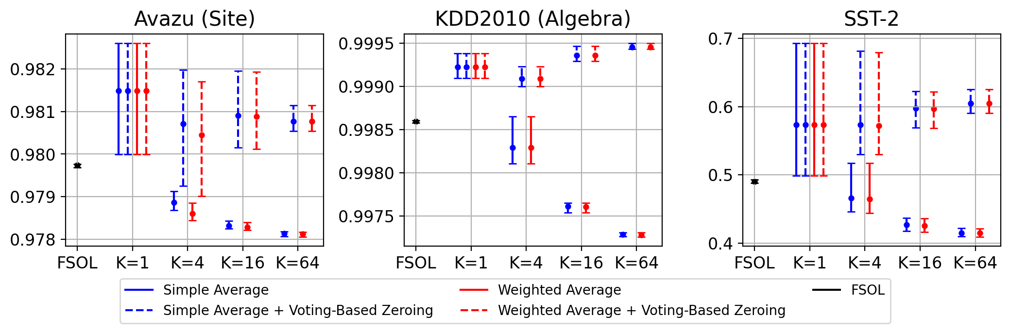
Preservation of sparsity. Finally, we aim to retain the favorable weight sparsity from FSOL. From Figure 4, we observe that even with reservoir size , the final sparsities achieved by FSOL-WRS are quite similar to that of base FSOL. Furthermore, we observe that with voting-based zeroing, FSOL-WRS often achieves even higher sparsity than the base model. Please see Appendix G.1 for additional errorbar-type plots and Appendix G.2 for sparsity over timestep. One explanation for why even FSOL-WRS variants without voting-based zeroing can achieve similar sparsity to base FSOL is that the final reservoir will likely contain candidate solutions from significantly earlier timesteps, when weights were sparser due to fewer aggressive updates. Thus, WAT can maintain sparsity despite the use of weight averaging.
4.2 Ablations and extensions
Top- ablation. A natural question that one might ask is — instead of probabilistically sampling candidate solutions, what if we deterministically picked the top- candidate solutions with the largest subsequent numbers of passive steps and took their simple and/or weighted average? Setting , we see from Table 3 that the best top- PAC/FSOL variants are not as effective as stabilizing test accuracy as the best PAC/FSOL-WRS variants, as shown in Table 2 and measured via ROP. Furthermore, Wilcoxon signed-rank test -values from Table 4 also suggest that this top- ablation cannot produce as statistically-significant increases in test accuracy stability compared to WAT, as measured via ROP. Like WAT, top- is also ineffective at producing statistically-significant increases in final test accuracy on PAC. On FSOL, top- can produce statistically significant increases in final test accuracy, but these -values are over an order of magnitude larger than FSOL-WRS’s (see Table 7 in Appendix F). As such, WAT is still the best for stabilizing test accuracy.
Relative Oracle Performance Final Test Accuracy Simple Average Weighted Average Simple Average Weighted Average PAC 0.162 0.0298 0.214 0.255 FSOL 0.00270 0.00270 0.0130 0.0130
Additional ablations and comparisons. For the interested reader, in Appendix D we include empirical performance comparisons of WRS-Augmented Training against two traditional ensembling mechanisms: moving average (e.g., averaging the most-recently-observed weight vectors at each timestep) and exponential average (e.g., forming an ensemble vector at each timestep), where is the base algorithm’s candidate solution at timestep . In short, especially in more real-world, large-scale settings where evaluation and checking are prohibitively expensive, WRS-Augmented Training is the fastest, most accurate, and most reliable method compared to all the aforementioned baselines.
Modifying WAT for non-passive aggressive methods. While the main theoretical and empirical results in this paper were primarily oriented towards passive-aggressive base models, in Appendix E, we include empirical simulations of applying a modified form of WRS-Augmented Training on top of three non-passive-aggressive online learning methods: Stochastic Gradient Descent with Momentum [40], ADAGRAD [14], and Truncated Gradient Descent [15]. In general, our modified WRS-Augmented Training effectively mitigates test accuracy when it exists, and does minimal harm when it does not.
5 Conclusion, limitations, and future work
In this paper, we introduced WRS-Augmented Training (WAT), a procedure that can be used to stabilize any passive-aggressive online learning algorithm, neither requiring a hold-out evaluation set nor additional passes over the training data. We applied WAT to base PAC and FSOL, demonstrating across 16 datasets that WAT is highly effective at mitigating the massive fluctuations in test accuracy between timesteps that affect many online learning algorithms. WAT runs at minimal cost, with only a fixed multiple on memory for multiple weight vectors to be saved.
One limitation of this work is that WAT implicitly assumes that the training and test data come from fixed distributions that do not change over time. However, some data distributions will evolve over time. As such, a candidate solution that entered the reservoir early on due to having a large number of subsequent passive steps might not actually retain its performance as the data distribution evolves over time. While they may eventually be replaced, non-IID adaptions may be useful in the future.
References
- [1] Peilin Zhao, Dayong Wang, Pengcheng Wu, and Steven CH Hoi. A Unified Framework for Sparse Online Learning. ACM Transactions on Knowledge Discovery from Data (TKDD), 14(5):1–20, 2020.
- [2] Nikos Karampatziakis and John Langford. Online Importance Weight Aware Updates, 2011.
- [3] Albert Bifet, Geoff Holmes, Bernhard Pfahringer, Philipp Kranen, Hardy Kremer, Timm Jansen, and Thomas Seidl. Moa: Massive online analysis, a framework for stream classification and clustering. In Proceedings of the first workshop on applications of pattern analysis, pages 44–50. PMLR, 2010.
- [4] Pavlos S Efraimidis and Paul G Spirakis. Weighted Random Sampling with a Reservoir. Information Processing Letters, 97(5):181–185, 2006.
- [5] Koby Crammer, Ofer Dekel, Joseph Keshet, Shai Shalev-Shwartz, and Yoram Singer. Online Passive-Aggressive Algorithms. Journal of Machine Learning Research, 7(19):551–585, 2006.
- [6] Edward Raff, Bobby Filar, and James Holt. Getting Passive Aggressive About False Positives: Patching Deployed Malware Detectors. In 2020 International Conference on Data Mining Workshops (ICDMW), pages 506–515. IEEE, nov 2020.
- [7] H. S. Anderson and P. Roth. EMBER: An Open Dataset for Training Static PE Malware Machine Learning Models. ArXiv e-prints, April 2018.
- [8] Richard Harang and Ethan M. Rudd. Sorel-20m: A large scale benchmark dataset for malicious pe detection. In Proceedings of the Conference on Applied Machine Learning for Information Security, 2021.
- [9] Robert J Joyce, Edward Raff, Charles Nicholas, and James Holt. MalDICT: Benchmark Datasets on Malware Behaviors, Platforms, Exploitation, and Packers. Proceedings of the Conference on Applied Machine Learning in Information Security, 2023.
- [10] Robert J Joyce, Edward Raff, and Charles Nicholas. A Framework for Cluster and Classifier Evaluation in the Absence of Reference Labels. In Proceedings of the 14th ACM Workshop on Artificial Intelligence and Security (AISec ’21). Association for Computing Machinery, 2021.
- [11] Robert J Joyce, Edward Raff, and Charles Nicholas. Rank-1 Similarity Matrix Decomposition For Modeling Changes in Antivirus Consensus Through Time. In Proceedings of the Conference on Applied Machine Learning for Information Security, 2021.
- [12] Robert J. Joyce, Tirth Patel, Charles Nicholas, and Edward Raff. AVScan2Vec: Feature Learning on Antivirus Scan Data for Production-Scale Malware Corpora. In Proceedings of the 16th ACM Workshop on Artificial Intelligence and Security, AISec ’23, page 185–196, New York, NY, USA, 2023. Association for Computing Machinery.
- [13] Koby Crammer, Alex Kulesza, and Mark Dredze. Adaptive Regularization of Weight Vectors. Machine learning, 91:155–187, 2013.
- [14] John Duchi, Elad Hazan, and Yoram Singer. Adaptive Subgradient Methods for Online Learning and Stochastic Optimization. Journal of Machine Learning Research, 12(7), 2011.
- [15] John Langford, Lihong Li, and Tong Zhang. Sparse Online Learning via Truncated Gradient. Journal of Machine Learning Research, 10(3), 2009.
- [16] Shai Shalev-Shwartz and Ambuj Tewari. Stochastic Methods for L1 Regularized Loss Minimization. In Proceedings of the 26th Annual International Conference on Machine Learning, pages 929–936, 2009.
- [17] Lin Xiao. Dual Averaging Method for Regularized Stochastic Learning and Online Optimization. Advances in Neural Information Processing Systems, 22, 2009.
- [18] Yoav Freund and Robert E Schapire. Large Margin Classification Using the Perceptron Algorithm. In Proceedings of the eleventh annual conference on Computational learning theory, pages 209–217, 1998.
- [19] Marco Muselli. On convergence properties of pocket algorithm. IEEE Transactions on Neural Networks, 8(3):623–629, 1997.
- [20] Nicolo Cesa-Bianchi, Alex Conconi, and Claudio Gentile. On the Generalization Ability of On-line Learning Algorithms. IEEE Transactions on Information Theory, 50(9):2050–2057, 2004.
- [21] Nicolo Cesa-Bianchi and Claudio Gentile. Improved Risk Tail Bounds for On-line Algorithms. IEEE Transactions on Information Theory, 54(1):386–390, 2008.
- [22] Ofer Dekel. From Online to Batch Learning with Cutoff-Averaging. Advances in Neural Information Processing Systems, 21, 2008.
- [23] Steve Wang and Will Cukierski. Click-Through Rate Prediction. Kaggle. https://kaggle.com/competitions/avazu-ctr-prediction, 2014.
- [24] Isabelle Guyon, Steve Gunn, Asa Ben-Hur, and Gideon Dror. Dexter. UCI Machine Learning Repository, 2008. DOI: https://doi.org/10.24432/C5P898.
- [25] Isabelle Guyon, Steve Gunn, Asa Ben-Hur, , and Gideon Dror. Dorothea. UCI Machine Learning Repository, 2008. DOI: https://doi.org/10.24432/C5NK6X.
- [26] J. Stamper, A. Niculescu-Mizil, S. Ritter, G.J. Gordon, and K.R. Koedinger. Algebra I 2008-2009. Challenge Data Set from KDD Cup 2010 Educational Data Mining Challenge. Find it at http://pslcdatashop.web.cmu.edu/KDDCup/downloads.jsp, 2010.
- [27] Jingwei Liang and Clarice Poon. Screening for Sparse Online Learning. arXiv preprint arXiv:2101.06982, 2021.
- [28] Gaëlle Loosli, Stéphane Canu, and Léon Bottou. Training Invariant Support Vector Machines using Selective Sampling. In Léon Bottou, Olivier Chapelle, Dennis DeCoste, and Jason Weston, editors, Large Scale Kernel Machines, pages 301–320. MIT Press, Cambridge, MA., 2007.
- [29] S Sathiya Keerthi, Dennis DeCoste, and Thorsten Joachims. A Modified Finite Newton Method for Fast Solution of Large Scale Linear SVMs. Journal of Machine Learning Research, 6(3), 2005.
- [30] Ken Lang. Newsweeder: Learning to Filter NetNews. In Proceedings of the Twelfth International Conference on Machine Learning, pages 331–339, 1995.
- [31] F. Pedregosa, G. Varoquaux, A. Gramfort, V. Michel, B. Thirion, O. Grisel, M. Blondel, P. Prettenhofer, R. Weiss, V. Dubourg, J. Vanderplas, A. Passos, D. Cournapeau, M. Brucher, M. Perrot, and E. Duchesnay. Scikit-learn: Machine Learning in Python. Journal of Machine Learning Research, 12:2825–2830, 2011.
- [32] Jundong Li, Kewei Cheng, Suhang Wang, Fred Morstatter, Robert P Trevino, Jiliang Tang, and Huan Liu. Feature Selection: A Data Perspective. ACM Computing Surveys (CSUR), 50(6):94, 2018.
- [33] David D Lewis, Yiming Yang, Tony Russell-Rose, and Fan Li. Rcv1: A New Benchmark Collection for Text Categorization Research. Journal of machine learning research, 5(Apr):361–397, 2004.
- [34] Richard Socher, Alex Perelygin, Jean Wu, Jason Chuang, Christopher D Manning, Andrew Y Ng, and Christopher Potts. Recursive Deep Models for Semantic Compositionality over a Sentiment Treebank. In Proceedings of the 2013 Conference on Empirical Methods in Natural Language Processing, pages 1631–1642, 2013.
- [35] Justin Ma, Lawrence K Saul, Stefan Savage, and Geoffrey M Voelker. Identifying Suspicious urls: An Application of Large-Scale Online Learning. In Proceedings of the 26th Annual International Conference on Machine Learning, pages 681–688, 2009.
- [36] John C Platt. Fast Training of Support Vector Machines Using Sequential Minimal Optimization. 1998.
- [37] Steve Webb, James Caverlee, and Calton Pu. Introducing the Webb Spam Corpus: Using Email Spam to Identify Web Spam Automatically. In CEAS, 2006.
- [38] Alessio Benavoli, Giorgio Corani, and Francesca Mangili. Should We Really Use Post-Hoc Tests Based on Mean-Ranks? Journal of Machine Learning Research, 17(5):1–10, 2016.
- [39] Janez Demšar. Statistical Comparisons of Classifiers over Multiple Data Sets. Journal of Machine Learning Research, 7(1):1–30, 2006.
- [40] Ilya Sutskever, James Martens, George Dahl, and Geoffrey Hinton. On the importance of initialization and momentum in deep learning. In International conference on machine learning, pages 1139–1147. PMLR, 2013.
- [41] David A Freedman. On tail probabilities for martingales. the Annals of Probability, pages 100–118, 1975.
Appendix A Proofs
A.1 Validity analysis
Proof of Theorem 1. The main statement involves two independent bounds. See the proofs for Theorem 5 and Theorem 6.
Theorem 5.
Let be the updated outputs of an online PA algorithm on inputs . Define and as previously. Also define as the minimal achievable risk of any model, such that almost surely.
Then
Proof.
First note that while is a constant value for any fixed , and are random variables induced by the distribution of . The sequence of observed samples affects both the algorithm’s output as well as the subsequent survival of .
Next, we define the event of interest . For a given realization of let the set . Then
We aim to split this into separate events and apply a union bound, but the contents and size of depend on .
Therefore we enumerate the models within each in the order they are received: , up to , enabling the index to refer to the corresponding model in any realization of . Then we can split the event that a hypothesis in the reservoir has longer survival into the union of events on each ordered hypothesis.
We have
To further clarify, the probabilities are computed over the probability space of , and depends on the realization of . Lemma 1 allows us to reason about the dependent model instances as independent geometric variables, but we need to extract into a instance-independent state. Thus we need to condition on the weight values, and then bound the probability uniformly across the expectation, using the premise that the weight risks are -distant. ∎
Theorem 6.
(Alternative bound) Let the same conditions hold as in Theorem 5. Then
Proof.
As before, let . Then
The event implies had or was tied for the highest survival, and we make the simplification that ties are resolved in favor of . Then
where in the third step, we apply Lemma 3. In the last step, we use the premise to suppose that there is at least one hypothesis which is -worse than .
Considering the first-term only,
∎
Remark.
Note that this gives the worst-case bound presuming no knowledge over the distribution of risks among the hypotheses. In such a scenario, the worst case is that all hypotheses achieve except for one which is . This is unrealistically adversarial, but the bound can easily be tightened by adding assumptions that the risks are well-behaved and applying those in the last step.
Lemma 1.
Let be the misclassification risk. Suppose an online learner outputs hypothesis at time after observing samples . Let be the subsequent survival time of , conditional on the observed sequence . Also let be the survival of over the distribution of sample sequences from . Then has a Geometric distribution with parameter . In addition .
Proof.
For the first statement, observe that when sampling independently from ,
Since each i.i.d. sample has a probability to be misclassified, the number of trials until the first misclassification is a Geometric distribution with parameter .
For the second, we need to consider a sequence of correct/incorrect classifications by as a Bernoulli process of r.v. with parameter , with a stopping time indicated by the first misclassification. is a random variable and we see that . Similarly can be defined on another Bernoulli process starting from . From the memoryless property, these have the same distribution. ∎
Lemma 2.
Given random variables and which are independent Geometric with parameters and respectively (e.g. PMF of is , then
and
Proof.
For the first statement,
For the second, note that
∎
Lemma 3.
Let be independent Geometric random variables with respective parameters . Let be independent. Then
Proof.
by independence. Substitute the PMF and CMFs of the geometric distribution to finish. ∎
Proof of Theorem 2.
Proof.
Note that
We now consider a subset of this event. We will compute the probability that and that . By definition, this latter event falls into .
For this to occur, note from Lemma 1 that each survival is drawn from a Geometric distribution. We want the chance that the largest survivals are from set and then the next largest is from . For additional simplicity, we further minimize the probability of this event by assigning all entries in risk and all entries in risk .
Conditioning on , all entries from are below except for one, which is equal to . There are ways to pick this largest one.
Then of the models in are also below , and are above . There are ways to choose such .
Finally this probability is summed over all values of . This is
As before, to get a simpler expression, we just consider , yielding
∎
We also discuss the additional assumption of this Theorem to show that it is readily satisfied.
Assumption. There is a partition of such that and , and that . That is, there is a set of good and bad models in terms of risk.
We can set to be any small number that satisfies a partition within the reservoir separating "good" from "bad" models – e.g. works. For demonstration, suppose the underlying risks of the models in the reservoir range from 0.1 to 0.3, with 0.1 being the best risk . Then . then contains the models with risks in and contains those with risks in . The only time this isn’t satisfied for any is if one of the partitions always ends up empty, which only happens if all the models have the same risk, a highly unlikely scenario where it is obvious that an ensemble isn’t needed.
A.2 Learning bounds
Our bound follows from the following lemma from [22]. This itself is based on martingale inequalities from [41] and developments in [21].
Lemma 4 (Dekel).
Let be a sequence of real-valued random variables and let be a sequence of random variables such that . Also assume that for all . Define , and let . Then for any and ,
From this we obtain our learning bound. The proof follows analogously to the one in [22], with modifications to handle our specific algorithm.
Proof of Theorem 3.
Proof.
In our method we have a reservoir containing models with associated weights . We focus on the case where the weight is equal to the passive steps survived by the model. To simplify this proof we consider a slightly modified algorithm, where all models with survival exceeding a threshold are included in the reservoir.
| (1) |
We rewrite the weighted average of the reservoir models as a function of the entire training sequence of length by defining to be 1 if is in and 0 otherwise. Furthermore on the first instance that joins , the is instead set to . This makes the weighting deterministic with respect to the information at time , at the cost of the reservoir size not being explicitly defined. While this is analogous to a top-k averaging scheme, the full WRS scheme will follow from the same reasoning, with a more complicated definition of . This is because all decision-making is performed using information that has already been seen.
Then we write , and our goal is to control . Furthermore, define the cumulative loss as . (We note that this term is a little different from the observed cumulative WRS loss because of the requirement of reweighting on the -th survival.)
In the lemma, let and let . Noting that is deterministic when conditioning on , the assumptions are met. Then with probability , we have .
Now , where the first equality uses the fact that is determined by the filtration , and the second similarly uses the conditioning information to fix and the i.i.d. assumption over .
Finally, we have from Jensen’s inequality.
Dividing the previous statement by , we put the pieces together to conclude
Finally, note that is the total time steps involved with the reservoir weights, which is at least with weights and the minimal survival time of the reservoir. Substituting completes the proof.
∎
Proof of Theorem 4.
Proof.
Combining the penultimate form of Theorem 3 (with instead of ) and the deduction that we have
Next, we turn our attention to the generic base-model online regret bound. From this we get .
We need to bound the cumulative loss of , that is , in terms of the risk: . Using an application of Hoeffding bound, we get
which holds with probability .
Combining the undesired tail events under the union bound, we get
with probability . As before, substitute in for to complete.
∎
Remark. The use of the online regret bound also indicates that the base models are improving over time. This means that their risks are decreasing, and hence the observed survival times are increasing. Thus even in the error term without in the denominator, is an increasing function of so we expect the error terms to decay in .
Appendix B Additional details on methods and experimental setups
B.1 Datasets
Of the 16 datasets used in our study (see Table 1), 14 are directly from existing repositories and/or literature, while 2 of them — Newsgroups (Binary, CS) and SST-2 — were modified from pre-existing assets. First, Newsgroups (binary, CS) was formed by taking the original multi-class Newsgroups dataset hosted in [31] and combining the labels “Computers" and “Science" as a class, and all other labels as the class. Second, SST-2 is a sentiment classification dataset originally containing text excerpts that we transformed into a linear classification dataset by using the CountVectorizer from [31].
B.2 Base PAC and FSOL hyperparameter tuning
We start our set of experiments by tuning the hyperparameter for base PAC, testing values in the set . For base FSOL, following Zhao et al.’s approach, we test values in and values in . For each dataset, we perform five runs of our base PAC and FSOL variants with randomized shuffles of the training and test data, running through the training data only once for each run. For each dataset, we pick the , , and values corresponding to the base PAC and FSOL variants, within the top 2.5% in terms of final test accuracy, that had the highest ROP, with all metrics averaged across the five runs. This experimental choice was made to strike a balance between simulating as difficult and risky conditions as possible and still choosing useful base model variants.
B.3 Metrics logging
Given that some of our datasets contain up to 36 million training points, it would be computationally and storage-wise unfeasible to record metrics at each timestep. As such, for each dataset, we record metrics at evenly-spaced timesteps (exact number depends on divisibility and integer division of by ) throughout the training stream, in addition to the initial and final timesteps. As such ROP was also approximated by proxying oracle accuracy by taking the cumulative maximum base model test accuracy across timesteps where metrics were recorded. As shown in the over-time figures in Appendix G.2, such a reduced resolution still tells us a very clear picture, while cutting down computation and storage requirements by many orders of magnitude.
B.4 Compute requirements and code availability
All experiments were run on a Linux computing cluster with 32 nodes, each with 40 Intel Xeon E5-2650 CPU cores and a total of 500 GB of RAM per node, managed using SLURM. Nonetheless, no experiments require multiprocessing or multiple cores. Depending on dataset size, some trials could take less than a minute to run, while the largest datasets would take a couple hours at max. However, larger datasets like Criteo will require 32 GB of RAM to load the dataset into memory.
Our source code for reproducing all experiments can be found at https://github.com/FutureComputing4AI/Weighted-Reservoir-Sampling-Augmented-Training/tree/main. All experiments were run on CPU.
Appendix C Applications to Malware Classification
Given that the original motivation for this work was a real-world need in malware detection, we present empirical results of PAC, PAC-WRS, FSOL, and FSOL-WRS on the EMBER malware classification dataset [7]. The EMBER dataset is comprised of features extracted from 1.1M benign and malicious Windows portable executable files and thus can be considered very close to a real-world test case of our WRS-Augmented Training method on a real-world deployment setting.
In Figure 5, we observe that both base PAC and FSOL experience significant and frequent test accuracy fluctuations throughout the training process. However, both PAC-WRS and FSOL-WRS very successfully mitigate these test accuracy fluctuations and even outperform the oracle model, all without the use of a separate validation set.

Indeed, WRS-Augmented Training is a promising tool towards stabilizing test accuracy performance in real-world deployment settings like malware detection.
Appendix D Comparisons to other ensembling and averaging schemes
One natural question a reader may ask is: how does WRS-Augmented Training compare to traditional weight-averaging schemes such as moving average (e.g., averaging the most-recently-observed weight vectors at each timestep) or exponential average (e.g., forming an ensemble vector at each timestep), where is the base algorithm’s candidate solution at timestep .
From Figures 6 and 7, we observe that the exponential average scheme is consistently ineffective at mitigating the test accuracy instabilities of the base models PAC and FSOL. The stability of the exponential average scheme is usually not much better than that of the base model, which makes sense because it still puts the majority of the weighting on the most recent candidate solution. From these figures, we also observe that the moving average also has very mixed effectiveness. Overall, we see that WRS-Augmented Training is more preferable to the moving average. This makes sense because with WRS-Augmented Training, we are much more selective about the quality of the candidate solutions that we retain in our reservoir, compared to moving average, which necessarily by definition must include poor-performing solutions as they appear.
Third, from Table 5222For Table 5, we are still waiting on a full set of results over multiple seeds for Criteo and Avazu (Site) for moving average, but because we are studying online algorithms, we can still share full-epoch results for one seed, and partial-epoch results for the other seeds as they exist today. We will update our paper accordingly when the results are finished. We also emphasize that the moving average method, on larger datasets, is multiple times slower per iteration, on average, than our WRS-Augmented Training, contributing to this delay. The general trends are already very clear from the results presented below., we see that for datasets with dimension , the moving average method can be significantly computationally slower per iteration than WRS-Augmented Training. For example, with PAC as the base model, the moving average method was, on average, x slower per iteration than WRS-Augmented Training on KDD2010 (Algebra) and x slower per iteration than WRS-Augmented Training on URL. Similar trends hold when using FSOL as the base algorithm. These results make sense because with WRS-Augmented Training, we do not always add candidate solutions to our reservoir for averaging, while with the moving average method, we must always add new candidate solutions into our set. These insertion and deletion costs will accrue over time. On smaller datasets, the moving average is faster or slower depending on the dataset, but runtime is dominated by IO and all methods finish within minutes. However, in more real-world, large-scale settings where evaluation and checking are prohibitively expensive, WRS-Augmented Training is the fastest, most accurate, and most reliable method compared to all the baselines.


PAC FSOL Dataset D Moving Avg. Expo. Avg. Moving Avg. Expo. Avg. Webspam 254 0.953 0.717 0.738 0.613 W8A 300 0.420 0.353 0.368 0.336 MNIST8 (4+9) 784 1.125 0.885 0.968 0.887 PCMAC 3289 0.483 0.312 0.377 0.235 SST-2 13757 0.903 0.431 0.748 0.411 Dexter 20000 0.577 0.143 0.285 0.066 Real-Sim 20958 0.949 0.624 0.707 0.564 RCV1 47236 1.825 0.892 1.366 1.011 Dorothea 100000 1.194 0.190000 0.580 0.254 Newsgroups (Binary, CS) 101631 3.587 1.042 1.376 0.543 Avazu (App) 1000000 8.357 2.507 8.078 2.544 Avazu (Site) 1000000 18.704 3.207 11.612 3.683 Criteo 1000000 14.267 2.876 7.009 2.381 News20 1355191 4.288 1.356 3.376 1.153 URL 3231961 10.050 3.945 9.124 4.058 KDD2010 (Algebra) 20216830 6.579 2.402 6.778 2.301
Appendix E Modified WRS-Augmented Training on non-passive aggressive online learning methods
In this section, we explore applying a modified form of WRS-Augmented Training (WAT) on top of three non-passive-aggressive online learning methods: Stochastic Gradient Descent with Momentum [40], ADAGRAD [14], and Truncated Gradient Descent [15], all using default hyperparameters. We emphasize that these three methods are not passive-aggressive as they always update their weight vectors at each time step, even if the data point was correctly classified. As such, the original WAT is not directly applicable.
However, we can modify WAT as follows. First, we define a pseudo-passive step as one where the current solution candidate made no classification error (i.e., no more concept of margin). Second, at a time step when the current solution candidate does make an error, we will sample the last weight vector before a mistake was made into our reservoir with probability proportional to the number of pseudo-passive steps, before resetting our counter. The rest of WAT operates as normal under this pseudo-passive step weighting.
From Figures 8 - 10, we observe that all three non-passive-aggressive online algorithms, in particular Stochastic Gradient Descent with Momentum (SGD+M) and Truncated Gradient Descent (TGD), are susceptible to experiencing concerning fluctuations in test accuracy. Consistently, across the algorithms, we observe that when such fluctuations are present, modified WAT effectively mitigates such fluctuations very well. On the other hand, when there is little fluctuation in the base model (e.g., see ADAGRAD), applying modified WAT will do little to no harm. We emphasize that WAT was not designed for non-passive-aggressive algorithms, but is still demonstrably useful and adaptable to a wider class of base models, which can constitute fruitful future work.


Appendix F Tables of -values for Wilcoxon Signed-Rank Tests
Below, we provide full tables of -values computed using Wilcoxon Signed-Rank Tests towards probing the statistical significance of the differences in ROP and final test accuracy between PAC/FSOL-WRS and their base model counterparts.
Simple Average Weighted Average Standard Exponential Standard Exponential PAC 0.0150 0.0199 0.0386 0.325 FSOL 0.000437 0.0879 0.000437 0.0787
Simple Average Weighted Average Standard Exponential Standard Exponential PAC 0.408 0.196 0.501 0.856 FSOL 0.00836 0.313 0.00836 0.679
Appendix G Additional results figures for PAC-WRS and FSOL-WRS
G.1 Uncertainty-quantified aggregate metrics across runs
Below, we provide figures with error bars (minimum and maximum across 5 trials) showing the relative oracle performances (ROP), final test accuracies, and final sparsities of PAC-WRS and FSOL-WRS alongside the base PAC and FSOL models, across all 16 datasets. The main takeaways are that a) PAC-WRS and FSOL-WRS overall incur substantially-lower ROP than their corresponding base models; b) PAC-WRS and FSOL-WRS overall achieve comparable, if not improved, final test accuracy compared to their corresponding base models, consistently with lower variance, too; c) the final sparsities of PAC-WRS and FSOL-WRS are overall comparable, if not higher than those of their corresponding base models.
G.1.1 FSOL and FSOL-WRS


G.1.2 PAC and PAC-WRS


G.2 Test accuracies and sparsities over time
Below, we provide figures showing test accuracies and sparsities over time on individual runs of PAC-WRS and FSOL-WRS, compared against their base model counterparts, on all 16 datasets. The main takeaways are that a) test accuracies over time on PAC-WRS and FSOL-WRS are overall much stabler, if not also higher, than their base model counterparts (and much closer to that of the oracle); b) applying WAT to PAC and FSOL does not significantly impact sparsity — in some cases, especially with voting-based zeroing, sparsity actually increases compared to the base model!
G.2.1 FSOL and FSOL-WRS


G.2.2 PAC and PAC-WRS


NeurIPS Paper Checklist
-
1.
Claims
-
Question: Do the main claims made in the abstract and introduction accurately reflect the paper’s contributions and scope?
-
Answer: [Yes]
-
Justification: Please see our Abstract and Introduction.
-
Guidelines:
-
•
The answer NA means that the abstract and introduction do not include the claims made in the paper.
-
•
The abstract and/or introduction should clearly state the claims made, including the contributions made in the paper and important assumptions and limitations. A No or NA answer to this question will not be perceived well by the reviewers.
-
•
The claims made should match theoretical and experimental results, and reflect how much the results can be expected to generalize to other settings.
-
•
It is fine to include aspirational goals as motivation as long as it is clear that these goals are not attained by the paper.
-
•
-
2.
Limitations
-
Question: Does the paper discuss the limitations of the work performed by the authors?
-
Answer: [Yes]
-
Justification: Please see Section 5.
-
Guidelines:
-
•
The answer NA means that the paper has no limitation while the answer No means that the paper has limitations, but those are not discussed in the paper.
-
•
The authors are encouraged to create a separate "Limitations" section in their paper.
-
•
The paper should point out any strong assumptions and how robust the results are to violations of these assumptions (e.g., independence assumptions, noiseless settings, model well-specification, asymptotic approximations only holding locally). The authors should reflect on how these assumptions might be violated in practice and what the implications would be.
-
•
The authors should reflect on the scope of the claims made, e.g., if the approach was only tested on a few datasets or with a few runs. In general, empirical results often depend on implicit assumptions, which should be articulated.
-
•
The authors should reflect on the factors that influence the performance of the approach. For example, a facial recognition algorithm may perform poorly when image resolution is low or images are taken in low lighting. Or a speech-to-text system might not be used reliably to provide closed captions for online lectures because it fails to handle technical jargon.
-
•
The authors should discuss the computational efficiency of the proposed algorithms and how they scale with dataset size.
-
•
If applicable, the authors should discuss possible limitations of their approach to address problems of privacy and fairness.
-
•
While the authors might fear that complete honesty about limitations might be used by reviewers as grounds for rejection, a worse outcome might be that reviewers discover limitations that aren’t acknowledged in the paper. The authors should use their best judgment and recognize that individual actions in favor of transparency play an important role in developing norms that preserve the integrity of the community. Reviewers will be specifically instructed to not penalize honesty concerning limitations.
-
•
-
3.
Theory Assumptions and Proofs
-
Question: For each theoretical result, does the paper provide the full set of assumptions and a complete (and correct) proof?
-
Answer: [Yes]
-
Guidelines:
-
•
The answer NA means that the paper does not include theoretical results.
-
•
All the theorems, formulas, and proofs in the paper should be numbered and cross-referenced.
-
•
All assumptions should be clearly stated or referenced in the statement of any theorems.
-
•
The proofs can either appear in the main paper or the supplemental material, but if they appear in the supplemental material, the authors are encouraged to provide a short proof sketch to provide intuition.
-
•
Inversely, any informal proof provided in the core of the paper should be complemented by formal proofs provided in appendix or supplemental material.
-
•
Theorems and Lemmas that the proof relies upon should be properly referenced.
-
•
-
4.
Experimental Result Reproducibility
-
Question: Does the paper fully disclose all the information needed to reproduce the main experimental results of the paper to the extent that it affects the main claims and/or conclusions of the paper (regardless of whether the code and data are provided or not)?
-
Answer: [Yes]
-
Guidelines:
-
•
The answer NA means that the paper does not include experiments.
-
•
If the paper includes experiments, a No answer to this question will not be perceived well by the reviewers: Making the paper reproducible is important, regardless of whether the code and data are provided or not.
-
•
If the contribution is a dataset and/or model, the authors should describe the steps taken to make their results reproducible or verifiable.
-
•
Depending on the contribution, reproducibility can be accomplished in various ways. For example, if the contribution is a novel architecture, describing the architecture fully might suffice, or if the contribution is a specific model and empirical evaluation, it may be necessary to either make it possible for others to replicate the model with the same dataset, or provide access to the model. In general. releasing code and data is often one good way to accomplish this, but reproducibility can also be provided via detailed instructions for how to replicate the results, access to a hosted model (e.g., in the case of a large language model), releasing of a model checkpoint, or other means that are appropriate to the research performed.
-
•
While NeurIPS does not require releasing code, the conference does require all submissions to provide some reasonable avenue for reproducibility, which may depend on the nature of the contribution. For example
-
(a)
If the contribution is primarily a new algorithm, the paper should make it clear how to reproduce that algorithm.
-
(b)
If the contribution is primarily a new model architecture, the paper should describe the architecture clearly and fully.
-
(c)
If the contribution is a new model (e.g., a large language model), then there should either be a way to access this model for reproducing the results or a way to reproduce the model (e.g., with an open-source dataset or instructions for how to construct the dataset).
-
(d)
We recognize that reproducibility may be tricky in some cases, in which case authors are welcome to describe the particular way they provide for reproducibility. In the case of closed-source models, it may be that access to the model is limited in some way (e.g., to registered users), but it should be possible for other researchers to have some path to reproducing or verifying the results.
-
(a)
-
•
-
5.
Open access to data and code
-
Question: Does the paper provide open access to the data and code, with sufficient instructions to faithfully reproduce the main experimental results, as described in supplemental material?
-
Answer: [Yes]
-
Justification: Please see our GitHub at https://github.com/FutureComputing4AI/Weighted-Reservoir-Sampling-Augmented-Training/tree/main, with a detailed README.md file.
-
Guidelines:
-
•
The answer NA means that paper does not include experiments requiring code.
-
•
Please see the NeurIPS code and data submission guidelines (https://nips.cc/public/guides/CodeSubmissionPolicy) for more details.
-
•
While we encourage the release of code and data, we understand that this might not be possible, so “No” is an acceptable answer. Papers cannot be rejected simply for not including code, unless this is central to the contribution (e.g., for a new open-source benchmark).
-
•
The instructions should contain the exact command and environment needed to run to reproduce the results. See the NeurIPS code and data submission guidelines (https://nips.cc/public/guides/CodeSubmissionPolicy) for more details.
-
•
The authors should provide instructions on data access and preparation, including how to access the raw data, preprocessed data, intermediate data, and generated data, etc.
-
•
The authors should provide scripts to reproduce all experimental results for the new proposed method and baselines. If only a subset of experiments are reproducible, they should state which ones are omitted from the script and why.
-
•
At submission time, to preserve anonymity, the authors should release anonymized versions (if applicable).
-
•
Providing as much information as possible in supplemental material (appended to the paper) is recommended, but including URLs to data and code is permitted.
-
•
-
6.
Experimental Setting/Details
-
Question: Does the paper specify all the training and test details (e.g., data splits, hyperparameters, how they were chosen, type of optimizer, etc.) necessary to understand the results?
-
Answer: [Yes]
-
Justification: Please see Algorithm 1, Section 4, and Appendix B, as well as our GitHub at https://github.com/FutureComputing4AI/Weighted-Reservoir-Sampling-Augmented-Training/tree/main.
-
Guidelines:
-
•
The answer NA means that the paper does not include experiments.
-
•
The experimental setting should be presented in the core of the paper to a level of detail that is necessary to appreciate the results and make sense of them.
-
•
The full details can be provided either with the code, in appendix, or as supplemental material.
-
•
-
7.
Experiment Statistical Significance
-
Question: Does the paper report error bars suitably and correctly defined or other appropriate information about the statistical significance of the experiments?
-
Answer: [Yes]
-
Guidelines:
-
•
The answer NA means that the paper does not include experiments.
-
•
The authors should answer "Yes" if the results are accompanied by error bars, confidence intervals, or statistical significance tests, at least for the experiments that support the main claims of the paper.
-
•
The factors of variability that the error bars are capturing should be clearly stated (for example, train/test split, initialization, random drawing of some parameter, or overall run with given experimental conditions).
-
•
The method for calculating the error bars should be explained (closed form formula, call to a library function, bootstrap, etc.)
-
•
The assumptions made should be given (e.g., Normally distributed errors).
-
•
It should be clear whether the error bar is the standard deviation or the standard error of the mean.
-
•
It is OK to report 1-sigma error bars, but one should state it. The authors should preferably report a 2-sigma error bar than state that they have a 96% CI, if the hypothesis of Normality of errors is not verified.
-
•
For asymmetric distributions, the authors should be careful not to show in tables or figures symmetric error bars that would yield results that are out of range (e.g. negative error rates).
-
•
If error bars are reported in tables or plots, The authors should explain in the text how they were calculated and reference the corresponding figures or tables in the text.
-
•
-
8.
Experiments Compute Resources
-
Question: For each experiment, does the paper provide sufficient information on the computer resources (type of compute workers, memory, time of execution) needed to reproduce the experiments?
-
Answer: [Yes]
-
Justification: Please see Appendix B.
-
Guidelines:
-
•
The answer NA means that the paper does not include experiments.
-
•
The paper should indicate the type of compute workers CPU or GPU, internal cluster, or cloud provider, including relevant memory and storage.
-
•
The paper should provide the amount of compute required for each of the individual experimental runs as well as estimate the total compute.
-
•
The paper should disclose whether the full research project required more compute than the experiments reported in the paper (e.g., preliminary or failed experiments that didn’t make it into the paper).
-
•
-
9.
Code Of Ethics
-
Question: Does the research conducted in the paper conform, in every respect, with the NeurIPS Code of Ethics https://neurips.cc/public/EthicsGuidelines?
-
Answer: [Yes]
-
Justification: We have carefully read the NeurIPS Code of Ethics and have made sure that our research conforms to it.
-
Guidelines:
-
•
The answer NA means that the authors have not reviewed the NeurIPS Code of Ethics.
-
•
If the authors answer No, they should explain the special circumstances that require a deviation from the Code of Ethics.
-
•
The authors should make sure to preserve anonymity (e.g., if there is a special consideration due to laws or regulations in their jurisdiction).
-
•
-
10.
Broader Impacts
-
Question: Does the paper discuss both potential positive societal impacts and negative societal impacts of the work performed?
-
Answer: [N/A]
-
Justification: This paper introduces a foundational research method that does not have any direct paths to negative societal impacts, aside from the general interactions of machine learning with society.
-
Guidelines:
-
•
The answer NA means that there is no societal impact of the work performed.
-
•
If the authors answer NA or No, they should explain why their work has no societal impact or why the paper does not address societal impact.
-
•
Examples of negative societal impacts include potential malicious or unintended uses (e.g., disinformation, generating fake profiles, surveillance), fairness considerations (e.g., deployment of technologies that could make decisions that unfairly impact specific groups), privacy considerations, and security considerations.
-
•
The conference expects that many papers will be foundational research and not tied to particular applications, let alone deployments. However, if there is a direct path to any negative applications, the authors should point it out. For example, it is legitimate to point out that an improvement in the quality of generative models could be used to generate deepfakes for disinformation. On the other hand, it is not needed to point out that a generic algorithm for optimizing neural networks could enable people to train models that generate Deepfakes faster.
-
•
The authors should consider possible harms that could arise when the technology is being used as intended and functioning correctly, harms that could arise when the technology is being used as intended but gives incorrect results, and harms following from (intentional or unintentional) misuse of the technology.
-
•
If there are negative societal impacts, the authors could also discuss possible mitigation strategies (e.g., gated release of models, providing defenses in addition to attacks, mechanisms for monitoring misuse, mechanisms to monitor how a system learns from feedback over time, improving the efficiency and accessibility of ML).
-
•
-
11.
Safeguards
-
Question: Does the paper describe safeguards that have been put in place for responsible release of data or models that have a high risk for misuse (e.g., pretrained language models, image generators, or scraped datasets)?
-
Answer: [N/A]
-
Justification: This paper does not involve any data or models that have a high risk for misuse.
-
Guidelines:
-
•
The answer NA means that the paper poses no such risks.
-
•
Released models that have a high risk for misuse or dual-use should be released with necessary safeguards to allow for controlled use of the model, for example by requiring that users adhere to usage guidelines or restrictions to access the model or implementing safety filters.
-
•
Datasets that have been scraped from the Internet could pose safety risks. The authors should describe how they avoided releasing unsafe images.
-
•
We recognize that providing effective safeguards is challenging, and many papers do not require this, but we encourage authors to take this into account and make a best faith effort.
-
•
-
12.
Licenses for existing assets
-
Question: Are the creators or original owners of assets (e.g., code, data, models), used in the paper, properly credited and are the license and terms of use explicitly mentioned and properly respected?
-
Answer: [Yes]
-
Justification: We enumerate and cite all datasets in Table 1. Aside from our own preprocessed versions of Newsgroups (Binary, CS) and SST-2, the 14 other datasets are all publicly available.
-
Guidelines:
-
•
The answer NA means that the paper does not use existing assets.
-
•
The authors should cite the original paper that produced the code package or dataset.
-
•
The authors should state which version of the asset is used and, if possible, include a URL.
-
•
The name of the license (e.g., CC-BY 4.0) should be included for each asset.
-
•
For scraped data from a particular source (e.g., website), the copyright and terms of service of that source should be provided.
-
•
If assets are released, the license, copyright information, and terms of use in the package should be provided. For popular datasets, paperswithcode.com/datasets has curated licenses for some datasets. Their licensing guide can help determine the license of a dataset.
-
•
For existing datasets that are re-packaged, both the original license and the license of the derived asset (if it has changed) should be provided.
-
•
If this information is not available online, the authors are encouraged to reach out to the asset’s creators.
-
•
-
13.
New Assets
-
Question: Are new assets introduced in the paper well documented and is the documentation provided alongside the assets?
-
Answer: [Yes]
-
Justification: Please see the README.md file in our accompanying GitHub https://github.com/FutureComputing4AI/Weighted-Reservoir-Sampling-Augmented-Training/tree/main.
-
Guidelines:
-
•
The answer NA means that the paper does not release new assets.
-
•
Researchers should communicate the details of the dataset/code/model as part of their submissions via structured templates. This includes details about training, license, limitations, etc.
-
•
The paper should discuss whether and how consent was obtained from people whose asset is used.
-
•
At submission time, remember to anonymize your assets (if applicable). You can either create an anonymized URL or include an anonymized zip file.
-
•
-
14.
Crowdsourcing and Research with Human Subjects
-
Question: For crowdsourcing experiments and research with human subjects, does the paper include the full text of instructions given to participants and screenshots, if applicable, as well as details about compensation (if any)?
-
Answer: [N/A]
-
Justification: No crowdsourcing or work with human subjects was performed for this paper.
-
Guidelines:
-
•
The answer NA means that the paper does not involve crowdsourcing nor research with human subjects.
-
•
Including this information in the supplemental material is fine, but if the main contribution of the paper involves human subjects, then as much detail as possible should be included in the main paper.
-
•
According to the NeurIPS Code of Ethics, workers involved in data collection, curation, or other labor should be paid at least the minimum wage in the country of the data collector.
-
•
-
15.
Institutional Review Board (IRB) Approvals or Equivalent for Research with Human Subjects
-
Question: Does the paper describe potential risks incurred by study participants, whether such risks were disclosed to the subjects, and whether Institutional Review Board (IRB) approvals (or an equivalent approval/review based on the requirements of your country or institution) were obtained?
-
Answer: [N/A]
-
Justification: This paper does not have any study participants and/or crowdsourcing.
-
Guidelines:
-
•
The answer NA means that the paper does not involve crowdsourcing nor research with human subjects.
-
•
Depending on the country in which research is conducted, IRB approval (or equivalent) may be required for any human subjects research. If you obtained IRB approval, you should clearly state this in the paper.
-
•
We recognize that the procedures for this may vary significantly between institutions and locations, and we expect authors to adhere to the NeurIPS Code of Ethics and the guidelines for their institution.
-
•
For initial submissions, do not include any information that would break anonymity (if applicable), such as the institution conducting the review.
-
•