Stability of strong viscous shock wave under periodic perturbation for 1-D isentropic navier-stokes system in the half space

Lin Chang School of Mathematical Sciences, Beihang University, Beijing, China [email protected] , Lin He College of Mathematics, Sichuan University, Chengdu, China [email protected] and Jin Ma School of Mathematics and Information Science, Shandong Technology and Business University, Yantai 264005, P. R. China [email protected]

Abstract.

In this paper, a viscous shock wave under space-periodic perturbation of 1-D isentropic Navier-Stokes system in the half space is investigated. It is shown that if the initial periodic perturbation around the viscous shock wave is small, then the solution time asymptotically tends to a viscous shock wave with a shift partially determined by the periodic oscillations. Moreover, the strength of the shock wave could be arbitrarily large. This result essentially improves the previous work ”A. Matsumura, M. Mei, Convergence to travelling fronts of solutions of the p-system with viscosity in the presence of a boundary. Arch. Ration. Mech. Anal. 146 (1999), no. 1, 1-22.” where the strength of shock wave is sufficiently small and the initial periodic oscillations vanish.

Key words and phrases:

Impermeable wall problem, Large amplitude shock, Space-periodic perturbation, Asymptotic stability

1. Introduction

We consider a one-dimensional isentropic Navier-Stokes system for a general viscous gas, i.e.,

\left\{\begin{array}[]{ll}v_{t}-u_{x}=0,&\\ u_{t}+p_{x}=(\mu(v)\frac{u_{x}}{v})_{x},&\end{array}\right.

(1.1)

where $v(x,t)$ is the specific volume, $u(x,t)$ the fluid velocity and $p=av^{-\gamma}$ is the pressure. Constant $a>0$ , $\gamma>1$ are adiabatic constants. $\mu(v)=\mu_{0}v^{-\alpha}$ is the viscosity coefficient with $\alpha\geq 0$ . Without loss of generality, we assume $\mu_{0}=1$ in what follows.

The system (1.1) is a basic system of hydrodynamic equations, it has a variety of wave phenomena, such as viscous shock waves and rarefaction waves. So it is important to study the stability of the viscous shock wave for system (1.1). The stability of viscous shock wave for the Cauchy problem has been extensively studied in a large literature since the pioneer works of [5, 22], see the other interesting works [4, 7, 9, 12, 13, 16, 17, 18, 20, 23, 27, 15] as the shock wave is weak.

Physicists and engineers are more concerned with the stability of large amplitude shock (strong shock). However, the stability of large amplitude shock (strong shock) is challenging in mathematics. There have been no research results of this area until the last few years.

In 2010, Matsumura-Wang [25] proved that the large amplitude shock wave is asymptotically stable by a clever weighted energy method as $\alpha>\frac{\gamma-1}{2}$ . In 2016, Vasseur-Yao [28] successfully removed the condition $\alpha>\frac{\gamma-1}{2}$ by introducing a new variable called “effective velocity”. Recently, He-Huang [6] extended the result of [28] to general pressure $p(v)$ and general viscosity $\mu(v)$ , where $\mu(v)$ could be any positive smooth function.

On the other hand, it is also interesting to investigate the stability of viscous shock waves for the initial-boundary value problem. In this paper, we considered an impermeable wall problem of (1.1) in the half space $x\geq 0$ , i.e.,

\left\{\begin{array}[]{ll}(v,u)(x,0)=(v_{0},u_{0})(x)\longrightarrow(v_{+}+\zeta(x),u_{+}+\varphi(x)),~{}x\rightarrow+\infty,&\\ u(0,t)=0,~{}~{}t\in{R_{+}},&\end{array}\right.

(1.2)

where $v_{+}>0,u_{+}<0$ . And $\left(\zeta,\varphi\right)$ are periodic functions with period $\pi>0$ and satisfy

\int_{0}^{\pi}\left(\zeta,\varphi\right)(x)dx=0.

(1.3)

When the periodic functions $\left(\zeta,\varphi\right)$ vanish, Matsumura-Mei [21] considered the impermeable wall problem (1.1), (1.2) in 1999. And recently, an interesting result by [3] considering the multi-dimensional case of this problem.

The impermeable wall means that the velocity at the boundary $x=0$ must be zero because there is no flow across the boundary. They showed in [21] that when $\alpha=0$ the solution of (1.1),(1.2) tends to a 2-viscous shock wave connecting the left state $(v_{-},0)$ and the right one $(v_{+},u_{+})$ provided that both the strength of shock and the initial perturbation are small and the 2-viscous shock is initially far away from the boundary, where $v_{-}$ is determined by the RH condition, i.e.,

\displaystyle\left\{\begin{array}[]{ll}-s_{2}(v_{+}-v_{-})-(u_{+}-u_{-})=0,&\\ -s_{2}(u_{+}-u_{-})+(p(v_{+})-p(v_{-}))=0.&\end{array}\right.

(1.6)

Moreover, we assume that $u_{-}=0$ . The condition that the strength of shock is small was removed from [2]. The condition that the shock is initially far away from the boundary was removed from [24]. How to remove both these two conditions mentioned above at the same time is still open. Let us briefly recall the idea of [24].

Since $u(0,t)=0$ at the boundary, we can exchange the impermeable wall problem (1.1) and (1.2) in the half space to the Cauchy problem in the whole space by defining $({{\tilde{v}}}(x,t),\tilde{u}(x,t))=(v(-x,t),-u(-x,t))$ as $x<0$ so that $(\tilde{v},\tilde{u})(x,t)$ still satisfies the system (1.1) in the whole space, i.e.,

\left\{\begin{array}[]{ll}\tilde{v}_{t}-\tilde{u}_{x}=0,&\\ \tilde{u}_{t}+p({\tilde{v}})_{x}=(\frac{{\tilde{u}}_{x}}{{\tilde{v}}^{\alpha+1}})_{x},~{}~{}x\in{R}&\end{array}\right.

(1.7)

equipped with the initial data

({\tilde{v}_{0}},{\tilde{u}_{0}})(x)=:({\tilde{v}},{\tilde{u}})(x,0)=\left\{\begin{array}[]{ll}(v_{0}(-x),-u_{0}(-x)),&x\leq 0,\\ (v_{0}(x),u_{0}(x)),&x\geq 0,\\ \end{array}\right.

(1.8)

satisfying

(\tilde{v}_{0},{\tilde{u}_{0}})(x)\rightarrow\left\{\begin{array}[]{ll}(v_{+},u_{+}),&(x\rightarrow+\infty),\\ (v_{+},-u_{+}),&(x\rightarrow-\infty).\end{array}\right.

(1.9)

Refer to caption — (a) Combination of the two shock waves

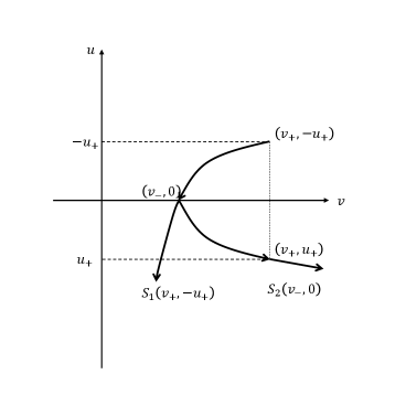
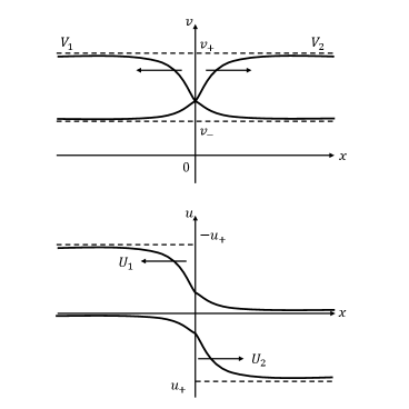
It is obvious that the solution of the Cauchy problem (1.7)-(1.9) confined in the half line $x>0$ is exactly the one of the impermeable wall problem (1.1),(1.2). In view of the far field states at $x=\pm\infty$ given by (1.9), it is expected that the solution to (1.7)-(1.9) asymptotically tends to a composite wave consisting of 1-viscous shock wave connecting $(v_{+},-u_{+})$ at the left and an intermediate state $(v_{\star},u_{\star})$ at the right, and 2-viscous shock wave connecting $(v_{\star},u_{\star})$ at the left and $(v_{+},u_{+})$ at the right. Fortunately $(v_{\star},u_{\star})=(v_{-},0)$ by the principle of RH condition and (1.9), see Fig (A), where $S_{1}(v_{+},-u_{+})$ means the 1-shock curve in the phase plane $(v,u)$ starting from the left state $(v_{+},-u_{+})$ and $S_{2}(v_{-},0)$ means the 2-shock curve in the phase plane $(v,u)$ starting from the left state $(v_{-},0)$ . The Figure B contains the graphs of the shock waves in the planes $(x,v)$ and $(x,u)$ . The wall $x=0$ can be regarded as a mirror and the 1-viscous shock is a mirror image of the 2-viscous shock in the plane $(x,v)$ , and the interaction between the 2-shock and the boundary $x=0$ for the impermeable wall problem (1.1)-(1.2) is replaced to consider the one between the 2-shock and its mirrored shock for the Cauchy problem (1.7)-(1.9).

In this paper, we want to improve the work of [2] where $\zeta=\varphi=0$ . Motivated by [24], the extended initial data in (1.8) satisfies

(\tilde{v}_{0},{\tilde{u}_{0}})(x)\rightarrow\left\{\begin{array}[]{ll}(v_{+}+\zeta(x),u_{+}+\varphi(x)),&(x\rightarrow+\infty),\\ (v_{+}+\zeta(-x),-u_{+}-\varphi(-x)),&(x\rightarrow-\infty).\end{array}\right.

(1.10)

We outline the strategy as follows. We apply the anti-derivative method to study the stability of the traveling wave solution $(V_{2}^{S},U_{2}^{S})(x-s_{2}t)$ , in which the anti-derivative of the perturbation ( $\tilde{v}-V_{2}^{S},\tilde{u}-U_{2}^{S}$ ), namely, $(\phi,\psi)(x,t)=\int_{-\infty}^{x}(\tilde{v}-V_{2}^{S},\tilde{u}-U_{2}^{S})(y,t)dy$ , “should” belong to some Sobolev spaces like $H^{2}(\mathbb{R})$ . However, the method above can not be applicable directly in this paper since ( $\tilde{v}-U_{2}^{S},\tilde{u}-U_{2}^{S}$ ) oscillates at the far field and hence does not belong to any $L^{p}$ space for $p\geq 1$ . Motivated by [30], we introduce a suitable ansatz $(V,U)(x,t)$ , which has the same oscillations as the solution $(\tilde{v},\tilde{u})(x,t)$ at the far field, so that $\int_{-\infty}^{x}(\tilde{v}-V,\tilde{u}-U)(x,t)dx$ belongs to some Sobolev spaces and the anti-derivative method is still available.

The rest of the paper will be arranged as follows. In Section 2, a suitable ansatz is constructed and the main results are stated. In Section 3, the stability problem is reformulated to a perturbation equation around the ansatz. In Section 4, the a priori estimates are established. In Section 5, the main results are proved. In Section 6, some complementary proofs are provided.

Notation. The functional $\|\cdot\|_{L^{p}(\Omega)}$ defined by $\|f\|_{L^{p}(\Omega)}=(\int_{\Omega}|f|^{p}(\xi){d\xi})^{\frac{1}{p}}$ . When $\Omega=(-\infty,\infty)$ , the symbol $\Omega$ is often omitted. As $p=2$ , we denote for simplicity,

\|f\|=\left(\int_{-\infty}^{\infty}f^{2}(\xi){d\xi}\right)^{\frac{1}{2}}.

In addition, $H^{m}$ denotes the $m$ -th order Sobolev space of functions defined by

\|f\|_{m}=\left(\sum_{k=0}^{m}\|\partial^{k}_{\xi}f\|^{2}\right)^{\frac{1}{2}}.

2. Preliminaries and the Main Theorem

2.1. Preliminaries

As pointed out by [21, 2], when perturbation functions $\zeta,\varphi$ vanish, the solution of the impermeable wall problem (1.1)-(1.2) is expected to tend toward the outgoing viscous shock $(V_{2}^{S},U_{2}^{S})(\xi_{2})$ satisfying

\left\{\begin{array}[]{ll}{-s_{2}}(V_{2}^{S})^{\prime}-(U_{2}^{S})^{\prime}=0,&\\ {-s_{2}}(U^{S}_{2})^{\prime}+p(V^{S}_{2})^{\prime}=\left(\frac{(U^{S}_{2})^{\prime}}{(V^{S}_{2})^{\alpha+1}}\right)^{\prime},&\\ (V^{S}_{2},U^{S}_{2})(-\infty)=(v_{-},0),\quad(V^{S}_{2},U^{S}_{2})(+\infty)=(v_{+},u_{+}),&\end{array}\right.

(2.1)

where ${}^{\prime}=d/d\xi_{2}$ , $\xi_{2}=x-s_{2}t$ , $s_{2}$ is the shock speed determined by the R-H condition (1.6) and $v_{\pm}>0,u_{+}<0$ are given constants. Using $(\ref{2.1})_{1}$ and $(\ref{2.1})_{2}$ , it follows that

\displaystyle\begin{split}&{s}_{2}^{2}(V^{S}_{2})^{\prime}+p(V^{S}_{2})^{\prime}=\left(\frac{-s_{2}(V^{S}_{2})^{\prime}}{(V^{S}_{2})^{\alpha+1}}\right)^{\prime}.\end{split}

(2.2)

Integrate (2.2) over $(-\infty,\xi_{2})$ . one has

\displaystyle\begin{split}&\frac{s_{2}(V^{S}_{2})^{\prime}}{(V^{S}_{2})^{\alpha+1}}=-{s}_{2}^{2}(V^{S}_{2})-p(V^{S}_{2})-b:=h(V^{S}_{2}),\quad V^{S}_{2}(\pm\infty)=v_{\pm},\end{split}

\displaystyle\begin{split}&U^{S}_{2}=-s_{2}(V^{S}_{2}-v_{-})=-s_{2}(V^{S}_{2}-v_{+})+u_{+},\end{split}

(2.3)

where $b=-s_{2}^{2}v_{-}-p(v_{-})=-s_{2}^{2}v_{+}-p(v_{+})$ . For abbreviation, we denote $s_{2}$ by $s$ . We have the following lemma.

Lemma 2.1 ([21]).

There exists a unique viscous shock $(V^{S}_{2},U^{S}_{2})(\xi_{2})$ up to a shift satisfying

\displaystyle 0<v_{-}<V^{S}_{2}(\xi_{2})<v_{+},\quad h(V^{S}_{2})>0,\quad(U^{S}_{2})^{\prime}<0,

\displaystyle\left|V^{S}_{2}(\xi)-v_{\pm}\right|=O(1)\theta e^{-c_{\pm}|\xi_{2}|},

(2.4)

as $\xi_{2}\rightarrow\pm\infty,$ where $\theta=\left|v_{+}-v_{-}\right|$ , $c_{\pm}=\frac{v_{\pm}^{\alpha+1}}{s}|p^{\prime}(v_{\pm})+s^{2}|$ , $s=\frac{-u_{+}}{v_{+}-v_{-}}.$

The initial data are assumed to satisfied

\displaystyle\begin{split}&v_{0}(x)-\zeta(x)-V_{2}^{S}(x-\beta_{1})\in L^{1}\cap H^{1}(R_{+}),\\ &u_{0}(x)-\varphi(x)-U_{2}^{S}(x-\beta_{1})\in L^{1}\cap H^{1}(R_{+}),\end{split}

(2.5)

and

u_{0}(0)=0

(2.6)

as compatibility condition, where $\beta_{1}>0$ is a constant. Set

\displaystyle(A_{0},B_{0})(x):=-\int_{x}^{\infty}(v_{0}(y)-\zeta(y)-V_{2}^{S}(y-\beta_{1}),u_{0}(y)-\varphi(y)-U_{2}^{S}(y-\beta_{1}))dy.

We further assume that

\displaystyle(A_{0},B_{0})\in L^{2}(R_{+}).

(2.7)

Borrowing from the idea of [24], we construct a composite wave. By [24], the mirrored shock $(V^{S}_{1},U^{S}_{1})(\xi_{1}),\xi_{1}=x-s_{1}t,s_{1}=-s$ , satisfies

\left\{\begin{array}[]{ll}{s}(V^{S}_{1})^{\prime}-{U^{S}_{1}}^{\prime}=0,&\\ {s}(U^{S}_{1})^{\prime}+p(V^{S}_{1})^{\prime}=(\frac{(U^{S}_{1})^{\prime}}{(V^{S}_{1})^{\alpha+1}})^{\prime},&\\ (V^{S}_{1},U^{S}_{1})(-\infty)=(v_{+},-u_{+}),\quad(V^{S}_{1},U^{S}_{1})(+\infty)=(v_{-},0).&\end{array}\right.

(2.8)

Thanks [21], one has

V^{S}_{1}(\xi)=V^{S}_{2}(-\xi),\quad U^{S}_{1}(\xi)=-U^{S}_{2}(-\xi),~{}~{}\forall\xi\in{R}.

(2.9)

The composite wave by two viscous shock weaves is defined as

\displaystyle\begin{split}\tilde{V}(x,t;\beta):=&V_{1}^{S}(x+st+\beta)+V^{S}_{2}(x-st-\beta)-v_{-},\\ \tilde{U}(x,t;\beta):=&U_{1}^{S}(x+st+\beta)+U^{S}_{2}(x-st-\beta),\end{split}

(2.10)

where $\beta$ is a constant. Motivated by [10, 8, 14, 11], we need two periodic solutions to (1.1) to establish the ansatz. Some properties of the solution are listed.

Lemma 2.2.

[11] Assume that $(v_{0},u_{0})(x)\in H^{k}(0,\pi)$ with $k\geq 2$ is periodic with period $\pi>0$ and average $(\bar{v},\bar{u}).$ Then there exists $\varepsilon_{0}>0$ such that if

\varepsilon_{1}:=\|{(v_{0},u_{0})-({\bar{v}},{\bar{u}})}\|_{H^{k}(0,\pi)}\leq\varepsilon_{0},

there exits a unique periodic solution

(v,u)(x,t)\in C\big{(}0,+\infty;H^{k}(0,\pi)\big{)}

to (1.1) with the initial data $(v,u)(x,0)=(v_{0},u_{0})(x),$ which has the average $({\bar{v}},{\bar{u}}),$ and satisfies

\|{(v,u)-({\bar{v}},{\bar{u}})}\|_{H^{k}(0,\pi)}(t)\leq C\varepsilon_{1}e^{-2\sigma_{0}t},\quad t\geq 0,

where the constants $C>0$ and $\sigma_{0}>0$ are independent of $\varepsilon_{1}$ and $t.$

2.2. Ansatz

In order to make the anti-derivative method is available, we choose a suitable pair of ansatz $(V,U)$ such that $\lim_{x\rightarrow\pm\infty}(v-V,u-U)(x,t)=(0,0)$ for any $t\geq 0$ . Motivated by [29], we define that the periodic solutions $\left(v_{l,r},u_{l,r}\right)$ of (1.1) as $x\rightarrow\mp\infty$ for all $t\geq 0,$ which have the periodic initial data:

\displaystyle\begin{split}&\left(v_{r},u_{r}\right)(x,0)=(v_{+},u_{+})+\left(\zeta,\varphi\right)(x),\\ &\left(v_{l},u_{l}\right)(x,0)=(v_{+},-u_{+})+\left(\zeta,-\varphi\right)(-x).\end{split}

For the viscous shocks $\left(V^{S}_{1},U^{S}_{1}\right)$ and $\left(V^{S}_{2},U^{S}_{2}\right),$ define

\displaystyle\begin{split}g_{1}(x)&:=\frac{V^{S}_{1}(x)-v_{+}}{v_{-}-v_{+}}=\frac{U^{S}_{1}(x)+u_{+}}{u_{+}},\\ g_{2}(x)&:=\frac{V^{S}_{2}(x)-v_{-}}{v_{+}-v_{-}}=\frac{U^{S}_{2}(x)}{u_{+}},\end{split}

(2.11)

where we have used the R-H condition (1.6). It is straightforward to check that $0\leq g_{i}(x)\leq 1$ and $g_{i}^{\prime}(x)>0$ for $i=1,2.$ With functions $v_{l,r},u_{l,r},g_{1,2}$ in hand, we are ready to construct the ansatz. Let $\mathcal{X}(t),\mathcal{Y}(t)$ are two $C^{1}$ curves on $[0,+\infty)$ which will be determined later. Set

	$\displaystyle V(x,t):={}$	$\displaystyle v_{l}(x,t)\left[1-g_{1}(x+st+{\mathcal{X}})\right]+v_{-}\left[g_{1}(x+st+{\mathcal{X}})-g_{2}(x-st-{\mathcal{X}})\right]$
		$\displaystyle+v_{r}(x,t)g_{2}(x-st-{\mathcal{X}}),$
	$\displaystyle U(x,t):={}$	$\displaystyle u_{l}(x,t)\left[1-g_{1}(x+st+{\mathcal{Y}})\right]+u_{r}(x,t)g_{2}(x-st-{\mathcal{Y}}).$

Plugging the ansatz $(V,U)$ into (1.1), we have

\begin{cases}V_{t}-U_{x}=(F_{1,1}+F_{1,2}+\mathcal{X}^{\prime}F_{1,3})_{x},&\\ U_{t}+p(V)_{x}-\mu\big{(}\frac{\partial_{x}U}{V}\big{)}_{x}=(F_{2,1}+F_{2,2}+\mathcal{Y}^{\prime}F_{2,3})_{x},&\end{cases}

(2.12)

where

F_{i,j}=\int_{-\infty}^{x}f_{i,j}(y,t)dy;i=1,2;\quad j=2,3,

\begin{cases}F_{1,1}=u_{l}\left[g_{1}(x+st+{\mathcal{Y}})-g_{1}(x+st+{\mathcal{X}})\right]\\ \qquad\quad-u_{r}\left[g_{2}(x-st-{\mathcal{Y}})-g_{2}(x-st-{\mathcal{X}})\right],\\ f_{1,2}=\left[-s(v_{l}-v_{+})+(u_{l}+u_{+})\right]g_{1}^{\prime}(x+st+{\mathcal{X}})\\ \qquad\quad-\left[s(v_{r}-v_{+})+(u_{r}-u_{+})\right]g_{2}^{\prime}(x-st-{\mathcal{X}}),\\ f_{1,3}=(v_{-}-v_{l})g_{1}^{\prime}(x+st+{\mathcal{X}})\\ \qquad\quad+(v_{-}-v_{r})g_{2}^{\prime}(x-st-{\mathcal{X}}),\end{cases}

and

\begin{cases}F_{2,1}=p(V)-p(v_{l})\left[1-g_{1}(x+st+{\mathcal{Y}})\right]-p(v_{r})g_{2}(x-st-{\mathcal{Y}})\\ \qquad\quad-\big{[}\frac{U_{x}}{V^{\alpha+1}}-\frac{u_{lx}}{v_{l}^{\alpha+1}}(1-g_{1}(x+st+{\mathcal{Y}}))-\frac{u_{rx}}{v_{r}^{\alpha+1}}g_{2}(x-st-{\mathcal{Y}})\big{]},\\ f_{2,2}=\big{[}-su_{l}-p(v_{l})+\frac{u_{lx}}{v_{l}^{\alpha+1}}\big{]}g^{\prime}_{1}(x+st+{\mathcal{Y}}))\\ \qquad\quad-\big{[}su_{r}-p(v_{r})+\frac{u_{rx}}{v_{r}^{\alpha+1}}\big{]}g_{2}^{\prime}(x-st-{\mathcal{Y}}),\\ f_{2,3}=-u_{l}g^{\prime}_{1}(x+st+{\mathcal{Y}}))-u_{r}g_{2}^{\prime}(x-st-{\mathcal{Y}}).\end{cases}

2.3. Location of The Shift ${\mathcal{X}}(t)$ and ${\mathcal{Y}}(t)$ .

To apply the anti-derivative method which is always used to study the stability of viscous shock, introduced in [26], we expect that

\displaystyle\begin{split}0=&\int_{-\infty}^{\infty}\left(\begin{array}[]{cccc}{\tilde{v}}(x,t)-V(x,t)\\ \tilde{u}(x,t)-U(x,t)\end{array}\right),\quad\forall t\geq 0.\end{split}

When $t=0$ , the shifts $\mathcal{X}(0)$ and $\mathcal{Y}(0)$ should satisfy

\displaystyle\begin{split}0=&\int_{-\infty}^{\infty}\left(\begin{array}[]{cccc}\tilde{v}_{0}(x)-V(x,0)\\ \tilde{u}_{0}(x)-U(x,0)\end{array}\right)dx:=\left(\begin{array}[]{cccc}I_{1}(\mathcal{X}(0))\\ I_{2}(\mathcal{Y}(0))\end{array}\right).\end{split}

(2.13)

Our next task is to show $\mathcal{X}(t),\mathcal{Y}(t)$ when $t>0$ . To make the system (2.12) as a conservative form, the curves $\mathcal{X}(t)$ and $\mathcal{Y}(t)$ should satisfy

\displaystyle\mathcal{X}^{\prime}(t)=-\lim_{x\rightarrow\infty}\frac{F_{1,2}(x,t)}{F_{1,3}(x,t)},~{}\mathcal{Y}^{\prime}(t)=-\lim_{x\rightarrow\infty}\frac{F_{2,2}(x,t)}{F_{2,3}(x,t)},

(2.14)

With the aid of (2.2), we know $F_{1,3}\neq 0,F_{2,3}\neq 0$ , provided that the initial periodic perturbations $\left(\zeta,\varphi\right)$ are small. Due to (1.8) and (2.9), $\tilde{u}_{0}(x),U(x,0)$ are odd functions and ${\tilde{v}}_{0}(x),V(x,0)$ are even functions, thus $I_{02}=0$ , i.e, we can choose any $\mathcal{Y}_{0}$ to guarantee that $I_{2}(\mathcal{Y}_{0})=0$ . For $I_{2}(\mathcal{X}_{0})=0$ , using (2.4) and (2.9), one gets that

\displaystyle\begin{split}I_{1}(\omega)=2&\int_{0}^{\infty}[v_{0}(x)-\tilde{q}(x)-V^{S}_{2}(x-\omega)]+[v_{-}-V^{S}_{1}(x+\omega)]dx\\ =2&\int_{0}^{\infty}[v_{0}(x)-\tilde{q}(x)-V^{S}_{2}(x-\omega)]dx-2\int_{0}^{\infty}\frac{1}{s}U^{S}_{1}(x+\omega)dx\\ =2&\int_{0}^{\infty}[{v}_{0}(x)-\tilde{q}(x)-V^{S}_{2}(x-\omega)]dx+2\int_{0}^{\infty}\frac{1}{s}U^{S}_{2}(-x-\omega)dx\\ =2&\int_{0}^{\infty}[{v}_{0}(x)-\tilde{q}(x)-V^{S}_{2}(x-\omega)]dx+2\int_{0}^{\infty}U^{S}_{2}(-st-\omega)dt.\end{split}

(2.15)

where

\displaystyle\begin{split}\tilde{q}(x)=&\zeta(-x)\left[1-g_{1}(x+\omega)\right]+\zeta(x)\left[g_{2}(x-\omega)\right].\end{split}

(2.16)

By directly calculate, we have $I_{1}(\infty)=\infty$ , $I_{1}(-\infty)=-\infty$ .

\displaystyle\begin{split}I_{1}^{\prime}(\omega)&=2\left\{(v_{+}-v_{-})-\int_{0}^{\infty}[\zeta(-x)g_{1}^{\prime}(x+\omega)+\zeta(x)g_{2}^{\prime}(x-\omega)]dx\right\}\\ &\geq 2\left\{(v_{+}-v_{-})-\|\zeta\|_{L_{\infty}}\int_{0}^{\infty}[g_{1}^{\prime}(x+\omega)+g_{2}^{\prime}(x-\omega)]dx\right\}\\ &\geq 2\left\{(v_{+}-v_{-})-2\varepsilon\right\}.\end{split}

(2.17)

Moreover, choosing $\varepsilon$ suitable small, we have $3(v_{+}-v_{-})\geq I_{1}^{\prime}(\omega)\geq v_{+}-v_{-}>0$ Thus there exists a unique constant $\mathcal{X}_{0}$ such that $I_{1}(\mathcal{X}_{0})=0$ . Moreover, using $I_{1}(\mathcal{X}_{0})=I_{1}(\beta_{1})+\int_{\beta_{1}}^{\mathcal{X}_{0}}I_{1}^{\prime}(s)ds$ , the constant $\mathcal{X}_{0}$ is between $\frac{1}{2}\tilde{M}+\beta_{1}$ and $\frac{3}{2}\tilde{M}+\beta_{1}$ , where

\displaystyle\begin{split}\tilde{M}=&\frac{1}{v_{-}-v_{+}}\left(\int_{0}^{\infty}[{v}_{0}(x)-\tilde{q}(x)-V^{S}_{2}(x-\beta_{1})]dx+\int_{0}^{\infty}U^{S}_{2}(-st-\beta_{1})dt\right)\\ =&\frac{1}{v_{-}-v_{+}}\left(\int_{0}^{\infty}[{v}_{0}(x)-\zeta(x)-V^{S}_{2}(x-\beta_{1})]dx+\int_{0}^{\infty}U^{S}_{2}(-st-\beta_{1})dt\right)\\ &-\frac{1}{v_{-}-v_{+}}\left(\int_{0}^{\infty}\left[\zeta(x)[g_{2}(x-\beta_{1})-1\right]+\zeta(-x)\left[1-g_{1}(x+\beta_{1})\right]dx\right)\\ \leq&\frac{1}{v_{-}-v_{+}}\left(\int_{0}^{\infty}[{v}_{0}(x)-\zeta(x)-V^{S}_{2}(x-\beta_{1})]dx+\int_{0}^{\infty}U^{S}_{2}(-st-\beta_{1})dt\right)+C\varepsilon,\end{split}

(2.18)

where we have used the following inequality

\displaystyle\begin{split}&\int_{0}^{\infty}\left[\zeta(x)[g_{2}(x-\beta_{1})-1\right]+\zeta(-x)\left[1-g_{1}(x+\beta_{1})\right]dx\\ =&\frac{-1}{(v_{-}-v_{+})}\int_{0}^{\infty}\zeta(x)\left[V^{S}_{2}(x-\beta_{1})-v_{+}\right]+\zeta(-x)\left[V^{S}_{1}(x+\beta_{1})-v_{-}\right]dx\\ \leq&C\|\zeta(x)\|_{L_{\infty}}\int_{0}^{\infty}\left|V^{S}_{2}(x-\beta_{1})-v_{+}\right|+\left|V^{S}_{1}(x+\beta_{1})-v_{-}\right|dx\leq C\varepsilon.\end{split}

(2.19)

By (2.5), we know $\tilde{M}$ exists. Thus we can obtain the curves $\mathcal{X}(t)$ and $\mathcal{Y}(t)$ . More precisely, it holds that

Lemma 2.3.

Assume that (1.3), (1.6) hold. Then there exists an $\varepsilon_{0}>0$ such that if

\|{\zeta}\|_{H^{2}(0,\pi)}+\|\varphi\|_{H^{2}(0,\pi)}<\varepsilon<\varepsilon_{0},

there exists a constant pair $(\mathcal{X},\mathcal{Y})(0)$ satisfying (2.13) where $\mathcal{X}(0)$ is uniquely determined and $\mathcal{Y}(0)$ can take any constant. Moreover, there exists a unique solution $(\mathcal{X},\mathcal{Y})(t)\in C^{1}(0,+\infty)$ to the system (2.14) with the fixed initial data $(\mathcal{X},\mathcal{Y})(0)=(\mathcal{X}_{0},\mathcal{Y}_{0}$ ) satisfying

|{\left(\mathcal{X}^{\prime},\mathcal{Y}^{\prime}\right)(t)}|+|{\left(\mathcal{X},\mathcal{Y}\right)(t)-\left(\mathcal{X}_{\infty},\mathcal{Y}_{\infty}\right)}|\leq C\varepsilon e^{-2\sigma_{0}t},\qquad t\geq 0.

Moreover, the corresponding constant locations $\mathcal{X}_{\infty},\mathcal{Y}_{\infty}$ as follows,

	$\displaystyle\mathcal{X}_{\infty}=~{}$	$\displaystyle\mathcal{X}_{0}+\frac{1}{2(v_{+}-v_{-})\pi}\left\{\int_{0}^{\pi}\int_{0}^{x}\zeta(y)-\zeta(-y)dydx\right.,$		(2.20)
		$\displaystyle\left.+2\pi\int_{0}^{+\infty}\left[\zeta(x)\left(1-g_{2}(x+\mathcal{X}_{0})\right)-\zeta(x)\left(1-g_{1}(x-\mathcal{X}_{0})\right)\right]dx\right\},$

and

$\displaystyle\mathcal{Y}_{\infty}=~{}$	$\displaystyle\mathcal{Y}_{0}+\frac{1}{2u_{+}\pi}\left\{\int_{0}^{\pi}\int_{0}^{x}\varphi(y)+\varphi(-y)dydx\right.$	(2.21)
	$\displaystyle-\int_{0}^{+\infty}\int_{0}^{\pi}\left[p(v_{l})-p({v}_{r})\right]dxdt$
	$\displaystyle\left.+\int_{0}^{\pi}g(v_{+}+\zeta(-x))-g(v_{+}+\zeta(x))dx\right\},$

where $g(v)=\frac{1}{\alpha}v^{-\alpha},$ if $\alpha\neq 0$ ; $g(v)=-\ln v$ , if $\alpha\neq 0$ .

Since the proof of Lemma 2.3 is similar to that in [29, 11], we put it in section 6.

2.4. the Main Result

We define

\displaystyle\begin{split}&\phi_{0}(x)=-\int^{\infty}_{x}\widetilde{v}_{0}(y)-V(y,0)dy,\\ &\psi_{0}(x)=-\int^{\infty}_{x}\widetilde{u}_{0}(y)-U(y,0)dy.\end{split}

In view of (2.13), we further assume that

\displaystyle(\phi_{0},\psi_{0})\in H^{2}(R).

(2.22)

Using the arbitrariness of $\mathcal{Y}_{0}$ , one can find a suitable $\mathcal{Y}_{0}$ , such that $\mathcal{X}_{\infty}=\mathcal{Y}_{\infty}$ . From now on, we denote $\beta:=\mathcal{X}_{\infty}=\mathcal{Y}_{\infty},\tilde{V}(x,t;\beta)=\tilde{V}(x,t),\tilde{U}(x,t;\beta)=\tilde{U}(x,t)$ for simple.

Lemma 2.4.

Suppose that (2.22) holds, there exists a positive constant $\delta_{1}$ such that if

\|\phi_{0}\|_{2}+\|\psi_{0}\|_{2}+\beta_{1}^{-1}+\varepsilon\leq\delta_{1},

then the Cauchy problem (1.7),(1.10) has a unique global solution $(\widetilde{v},\widetilde{u})(x,t)$ satisfying

\displaystyle\begin{split}&{\widetilde{v}(x,t)}-V(x,t)\in C^{0}([0,+\infty);H^{1})\cap L^{2}([0,+\infty);H^{2}),\\ &{\widetilde{u}(x,t)}-U(x,t)\in C^{0}([0,+\infty);H^{1})\cap L^{2}([0,+\infty);H^{1}),\\ \end{split}

(2.23)

and

\displaystyle\begin{split}&\sup_{x\in{R}}|{\widetilde{v}(x,t)}-V(x,t)|\rightarrow 0,\text{ as }t\rightarrow+\infty,\\ &\sup_{x\in{R}}|{\widetilde{u}(x,t)}-U(x,t)|\rightarrow 0,\text{ as }t\rightarrow+\infty.\end{split}

(2.24)

Now, we turn to the original initial-value problem. Our main theorem is:

Theorem 2.1.

For any given constants $u_{+}<0$ and $v_{+}>0$ , if (2.5)-(2.7) hold. There exists a positive constant $\delta_{2}$ such that if

\|A_{0}\|_{H^{2}({R}_{+})}+\|B_{0}\|_{H^{2}({R}_{+})}+\beta_{1}^{-1}+\varepsilon\leq\delta_{2},

then the IBVP (1.1), (1.2) has a unique global solution $(v,u)(x,t)$ , satisfying

\displaystyle\begin{split}&\sup_{x\in{R}_{+}}|{(v,u)(x,t)}-(V^{S}_{2},U^{S}_{2})(x-st-\beta)|\rightarrow 0,\text{as }t\rightarrow+\infty,\end{split}

where $\beta$ is determined by (2.20).

3. Reformulation of the Original Problem

Set

\displaystyle\begin{split}\phi&(x,t):=\int^{x}_{-\infty}{(\tilde{v}-V)}(y,t){d}y,\\ \psi&(x,t):=\int^{x}_{-\infty}{(\tilde{u}-U)}(y,t){d}y.\end{split}

Thus $(\tilde{v},\tilde{u})(x,t)$ satisfy

	$\displaystyle\tilde{v}$	$\displaystyle(x,t)=\phi_{x}(x,t)+V(x,t),$
	$\displaystyle\tilde{u}$	$\displaystyle(x,t)=\psi_{x}(x,t)+U(x,t).$

From $(\ref{2.8})$ , we know the ansazt $(V,U)$ satisfies

\left\{\begin{array}[]{ll}{V}_{t}-{U}_{x}=-F_{1x},&\\ U_{t}+p(V)_{x}-\left(\frac{U_{x}}{V^{\alpha+1}}\right)_{x}=-F_{2x},&\\ (V,U)(\pm\infty,t)=(v_{+},\pm u_{+}),&\end{array}\right.

(3.1)

where

	$\displaystyle F_{1}(x,t)$	$\displaystyle:=-F_{1,1}(x,t)-F_{1,2}(x,t)-\mathcal{X}^{\prime}(t)F_{1,3}(x,t),$		(3.2)
	$\displaystyle F_{2}(x,t)$	$\displaystyle:=-F_{2,1}(x,t)-F_{2,2}(x,t)-\mathcal{Y}^{\prime}(t)F_{2,3}(x,t).$		(3.2)

Motivated by [21] and [1], with the help of (3.1) and (1.1), it follows that

\left\{\begin{array}[]{ll}\phi_{t}-\psi_{x}=F_{1},&\\ \psi_{t}-f(V,U_{x})\phi_{x}-\frac{\psi_{xx}}{V^{\alpha+1}}=F_{2}+J.&\end{array}\right.

(3.3)

The initial condition satisfies

\displaystyle\left(\phi_{0},\psi_{0}\right)

\displaystyle(x)\in{H}^{2},\quad x\in{R},

(3.4)

where

\displaystyle f(V,U_{x})=-p^{\prime}(V)-(\alpha+1)\frac{U_{x}}{V^{\alpha+2}},

(3.5)

\displaystyle J

\displaystyle=\frac{{u}_{x}}{{v}^{\alpha+1}}-\frac{U_{x}}{V^{\alpha+1}}-\frac{\psi_{xx}}{V^{\alpha+1}}+(\alpha+1)\frac{U_{x}\phi_{x}}{V^{\alpha+2}}-\left[p({v})-p(V)-p^{\prime}(V)\phi_{x}\right].

(3.6)

Lemma 3.1.

Under the assumptions of Theorem 2.1, the anti-derivative variables (3.2) exist and satisfy that

\|{F_{1}}\|_{2}\leq C\varepsilon e^{-\sigma_{0}t},\|F_{2}\|_{1}\leq C\varepsilon e^{-\sigma_{0}t}+Ce^{-c_{-}\beta_{1}}e^{-sc_{-}t}.

The proof is based on Lemma 2.2, Lemma 2.3 and Lemma 5.2 and we place it in section 6 for brevity.

We will seek the solution in the functional space ${X}_{\delta}(0,T)$ for any $0\leq T<+\infty$ ,

\displaystyle\begin{split}{X}_{\delta}(0,T):=&\left\{(\phi,\psi)\in C([0,T];{H}^{2})|\phi_{x}\in{L}^{2}(0,T;{H}^{1}),\psi_{x}\in{L}^{2}(0,T;{H}^{2})\right.\\ &\sup_{0\leq t\leq T}\|(\phi,\psi)(t)\|_{2}\leq\delta\},\end{split}

where ${\delta}\ll 1$ is small.

Remark 3.1.

The function space is well defined because the Dirac function will not appear in $\phi,\phi_{x},\phi_{xx},\psi,\psi_{x},\psi_{xx},\psi_{xxx}$ , which can be guaranteed by $u(0)=0$ .

Proposition 3.1.

(A priori estimate) For some time $T>0$ , if $(\phi,\psi)\in{X}_{\delta}(0,T)$ is the solution of (3.3), (3.4). Then there exists a positive constant $\delta_{0}$ independent of $T$ , such that if

\sup_{0\leq t\leq T}\|(\phi,\psi)(t)\|_{{2}}\leq\delta\leq\delta_{0},

for $t\in[0,T]$ , then

\displaystyle\|(\phi,\psi)(t)\|_{{2}}^{2}+\int_{0}^{t}(\|\phi_{x}(t)\|^{2}_{1}+\|\psi_{x}(t)\|_{2}^{2}){d}t\leq C_{0}(\|(\phi_{0},\psi_{0})\|_{{2}}^{2}+e^{-c_{-}\beta_{1}}+\varepsilon),

where $C_{0}>1$ ia a constant independent of $T$ .

Once Proposition 3.1 is obtained, the local solution $(\phi,\psi)$ can be extend to $T=+\infty.$ See the following lemma.

Lemma 3.2.

If $(\phi_{0},\psi_{0})\in{H}^{2}$ , there exists a positive constant $\delta_{1}=\frac{\delta_{0}}{\sqrt{C_{0}}}$ , such that if

\|(\phi_{0},\psi_{0})\|_{{2}}^{2}+e^{-c_{-}\beta_{1}}+\varepsilon\leq\delta_{1}^{2},

then the initial value problem (3.3), (3.4) has a unique global solution $(\phi,\psi)\in{X}_{\delta_{0}}(0,\infty)$ satisfying

\displaystyle\sup_{t\geq 0}\|(\phi,\psi)(t)\|_{{2}}^{2}+\int_{0}^{\infty}(\|\phi_{x}(t)\|^{2}_{1}+\|\psi_{x}(t)\|_{2}^{2}){d}t\leq C_{0}(\|(\phi_{0},\psi_{0})\|_{{2}}^{2}+e^{-c_{-}\beta_{1}}+\varepsilon).

4. A Priori Estimate

For some $T>0$ , the problem $(\ref{3.3}),(\ref{3.4})$ is assumed that has a solution $(\phi,\psi)\in{X}_{\delta}(0,T)$ in this section.

\displaystyle\sup_{0\leq t\leq T}\|(\phi,\psi)(t)\|_{2}\leq\delta.

(4.1)

The Sobolev inequality gives that $\frac{1}{2}v_{-}\leq v\leq\frac{3}{2}v_{+}$ , and

\displaystyle\sup_{0\leq t\leq T}\{\|(\phi,\psi)(t)\|_{{L}^{\infty}}+\|(\phi_{x},\psi_{x})(t)\|_{{L}^{\infty}}\}\leq{\delta}.

Motivated by [28], we introduce the new effective velocity $\widetilde{h}=\widetilde{u}-\widetilde{v}^{-(\alpha+1)}\widetilde{v}_{x}$ . It holds that

\left\{\begin{array}[]{ll}\widetilde{v}_{t}-\widetilde{h}_{x}=(\frac{\widetilde{v}_{x}}{\widetilde{v}^{\alpha+1}})_{x},&\\ \widetilde{h}_{t}+\widetilde{p}_{x}=0.&\end{array}\right.

(4.2)

Similarly, we define $H=U-V^{-(\alpha+1)}V_{x}$ , then (3.1) becomes

\left\{\begin{array}[]{ll}V_{t}-H_{x}=\left(\frac{V_{x}}{V^{\alpha+1}}\right)_{x}-F_{1,x},&\\ H_{t}+p(V)_{x}=-F_{2,x}.&\end{array}\right.

(4.3)

We define

\displaystyle\int_{-\infty}^{x}(\widetilde{h}-H){dx}=\Psi.

(4.4)

Substitute (4.3) from (4.2) and integrate the resulting system with respect to $x$ . Using (4.4), we have

\left\{\begin{array}[]{ll}\phi_{t}-\Psi_{x}-\frac{\phi_{xx}}{V^{\alpha+1}}=G+{F}_{1},&\\ \Psi_{t}+p^{\prime}(V)\phi_{x}=-p(\tilde{v}|V)+F_{2}-\frac{F_{1x}}{V^{\alpha+1}},&\end{array}\right.

(4.5)

where

\displaystyle G=\frac{\widetilde{v}_{x}}{\widetilde{v}^{\alpha+1}}-\frac{V_{x}}{V^{\alpha+1}}-\frac{\phi_{xx}}{V^{\alpha+1}},\quad p(\widetilde{v}|V)=\left(p(\widetilde{v})-p(V)\right)-p^{\prime}(V)\phi_{x}.

Now we give some lemmas that are useful in energy estimate.

Lemma 4.1.

([6, 21]) Under the assumption of (4.1), we have

\displaystyle\begin{split}&p(\widetilde{v}|V)\leq C\phi_{x}^{2},\quad|p(\widetilde{v}|V)_{x}|\leq C(|\phi_{xx}\phi_{x}|+|V_{x}|\phi_{x}^{2}),\\ &|G|\leq C(|\phi_{xx}\phi_{x}|+|V_{x}|\phi_{x}),\\ \end{split}

(4.6)

and

\displaystyle\begin{split}&|J|\leq C(\phi_{x}^{2}+|\phi_{x}\psi_{xx}|),\\ &|J_{x}|\leq C(\phi_{x}^{2}+|\phi_{x}\phi_{xx}|+|\psi_{xx}\phi_{xx}|+|\psi_{xxx}\phi_{x}|+|\phi_{x}\psi_{xx}|).\end{split}

(4.7)

Lemma 4.2.

The error terms

\displaystyle\begin{split}q(x,t):=V(x,t)-\tilde{V}(x,t);\quad z(x,t):=U(x,t)-\tilde{U}(x,t),\end{split}

(4.8)

satisfy

\|(z,q)(.,t)\|_{2}\leq C\varepsilon e^{-2\sigma_{0}t}.

Proof.

By direct calculate, one gets that

\displaystyle\begin{split}q(x,t):=&(v_{l}-v_{+})(x,t)\left[1-g_{1}(x+st+{\mathcal{X}})\right]+(v_{r}-v_{+})(x,t)g_{2}(x-st-{\mathcal{X}})\\ &+V_{1}^{S}(x+st+{\mathcal{X}})+V^{S}_{2}(x-st-{\mathcal{X}})-V_{1}^{S}(x+st+\beta)-V^{S}_{2}(x-st-\beta)\\ \leq&C(|v_{l}-{v}_{+}|+|v_{r}-{v}_{+}|+|{\mathcal{X}}-\beta|),\end{split}

(4.9)

and

\displaystyle\begin{split}\frac{\partial^{k}q}{\partial x^{k}}\leq C\left(\left|\frac{\partial^{k}v_{l}}{\partial x^{k}}\right|+\left|\frac{\partial^{k}v_{r}}{\partial x^{k}}\right|+\left|{\mathcal{X}}-\beta\right|\right),\quad k=1,2.\end{split}

(4.10)

With the aid of Lemma 2.2 and Lemma 2.3, one gets that

\|q\|_{2}\leq C\varepsilon e^{-2\sigma_{0}t}.

(4.11)

Similar, we obtain

\|z\|_{2}\leq C\varepsilon e^{-2\sigma_{0}t}.

(4.12)

∎

4.1. Low Order Estimates.

Lemma 4.3.

Under the same assumptions of Proposition 3.1, we have

\displaystyle\begin{split}&\|(\phi,\Psi)\|^{2}(t)+\int_{0}^{t}\int_{-\infty}^{\infty}\sqrt{-\tilde{U}_{x}}\Psi^{2}dxdt+\int_{0}^{t}\|\phi_{x}\|^{2}dt\\ \leq&C\|(\phi_{0},\Psi_{0})\|^{2}+C{\delta}\int_{0}^{t}\|\phi_{xx}\|^{2}dt+Ce^{-c_{-}\beta_{1}}+C\varepsilon.\end{split}

Proof.

We multiply $(\ref{4.5})_{1}$ and $(\ref{4.5})_{2}$ by $\phi$ and $\frac{\Psi}{-p^{\prime}(V)}$ , respectively, sum them up, and intergrading result with respect to $t$ and $x$ over $[0,t]\times{R}$ , we have

	$\displaystyle\frac{1}{2}\int_{-\infty}^{\infty}\left(\phi^{2}-\frac{\Psi^{2}}{p^{\prime}(V)}\right)dx+\int_{0}^{t}\int_{-\infty}^{\infty}\frac{-p^{\prime\prime}(V)}{2(p^{\prime}(V))^{2}}\tilde{U}_{x}\Psi^{2}+\frac{\phi_{x}^{2}}{V^{\alpha+1}}dxdt$
$\displaystyle=$	$\displaystyle\frac{1}{2}\left.\int_{-\infty}^{\infty}\left(\phi^{2}-\frac{\Psi^{2}}{p^{\prime}(V)}\right)dx\right\|_{t=0}$
	$\displaystyle+\int_{0}^{t}\int_{-\infty}^{\infty}\left[G+(\alpha+1)\frac{V_{x}\phi_{x}}{V^{\alpha+2}}\right]\phi+\frac{p(\tilde{v}\|V)\Psi}{p^{\prime}(V)}dxdt$	(4.13)
	$\displaystyle+\int_{0}^{t}\int_{-\infty}^{\infty}F_{1}\phi-\frac{\Psi}{p^{\prime}(V)}\left(F_{2}-\frac{F_{1x}}{V^{\alpha+1}}\right)dxdt$
	$\displaystyle+\frac{1}{2}\int_{0}^{t}\int_{-\infty}^{\infty}\frac{p^{\prime\prime}(V)}{p^{\prime}(V)^{2}}(z-F_{1})_{x}\Psi^{2}dxdt$
$\displaystyle:=$	$\displaystyle\frac{1}{2}\left.\int_{-\infty}^{\infty}\left(\phi^{2}-\frac{\Psi^{2}}{p^{\prime}(V)}\right)dx\right\|_{t=0}+\sum_{i=1}^{3}A_{i}.$	(4.14)

By direct calculate, one gets that

\left|G+(\alpha+1)\frac{V_{x}\phi_{x}}{V^{\alpha+2}}\right|\leq C|\phi_{x}|(\phi_{x}^{2}+\phi_{xx}^{2}).

(4.15)

Due to (4.6), (4.15), we can get

\displaystyle\begin{split}A_{1}\leq&C\int_{0}^{t}\|\phi\|_{L^{\infty}}\left\|\phi_{x}(\phi_{x}^{2}+\phi_{xx}^{2})\right\|_{L^{1}}dt+C\int_{0}^{t}\|\Psi\|_{L^{\infty}}\|\phi_{x}^{2}\|_{L^{1}}dt\\ \leq&C\delta\int_{0}^{t}\|\phi_{x}\|^{2}+\|\phi_{xx}\|^{2}dt.\end{split}

(4.16)

With the aid of Lemma 3.1, H $\mathrm{\ddot{o}}$ lder inequality, we have

\begin{split}A_{2}\leq&C\int_{0}^{t}\|\phi,\Psi\|(\|F_{1}\|_{1}+\|F_{2}\|)dt\\ \leq&C\sup_{\tau\in[0,t]}(\|\phi,\Psi\|^{2}+1)\int_{0}^{t}\|F_{1}\|_{1}+\|F_{2}\|dt\\ \leq&C(\varepsilon+e^{-c_{-}\beta_{1}}).\end{split}

(4.17)

Using H $\mathrm{\ddot{o}}$ lder inequality, Sobolev inequality, combining Lemma 3.1, Lemma 4.2, one gets

\displaystyle\begin{split}A_{3}\leq&C\int_{0}^{t}\|(z-F_{1})_{x}\|_{L^{\infty}}\|\Psi^{2}\|_{L^{1}}dt\\ \leq&C\sup_{\tau\in[0,t]}\|\Psi(\tau)\|^{2}\int_{0}^{t}\|(z-F_{1})_{x}\|_{H^{1}}dt\leq C\varepsilon.\end{split}

(4.18)

Inserting (4.16)-(4.18) into (4.13), using the smallness of $\delta$ , we obtain the proof of Lemma 4.3. ∎

Lemma 4.4.

Under the same assumptions of Proposition 3.1, we have

\displaystyle\|(\phi,\Psi)(t)\|_{1}^{2}+\int_{0}^{t}\|\phi_{x}\|_{1}^{2}{dt}\leq C\|(\phi_{0},\Psi_{0})\|_{1}^{2}+Ce^{-c_{-}\beta_{1}}+C\varepsilon.

Proof.

We multiply $(\ref{4.5})_{1}$ and $(\ref{4.5})_{2}$ by $-\phi_{xx}$ and $\frac{\Psi_{xx}}{p^{\prime}(V)}$ , respectively and sum over the result, intergrade the result with respect to $t$ and $x$ over $[0,t]\times{R}$ , we have

	$\displaystyle\frac{1}{2}\int_{-\infty}^{\infty}\left(\phi_{x}^{2}-\frac{\Psi_{x}^{2}}{p^{\prime}(V)}\right)dx+\int_{0}^{t}\int_{-\infty}^{\infty}\frac{-p^{\prime\prime}(V)}{2(p^{\prime}(V))^{2}}\tilde{U}_{x}\Psi_{x}^{2}+\frac{\phi^{2}_{xx}}{V^{\alpha+1}}dxdt$
$\displaystyle=$	$\displaystyle\frac{1}{2}\int_{-\infty}^{\infty}\left.\left(\phi_{x}^{2}-\frac{\Psi_{x}^{2}}{p^{\prime}(V)}\right)dx\right\|_{t=0}+\int_{0}^{t}\int_{-\infty}^{\infty}\frac{p^{\prime\prime}(V)}{p^{\prime}(V)}\tilde{V}_{x}\Psi_{x}\phi_{x}dxdt$
	$\displaystyle+\int_{0}^{t}\int_{-\infty}^{\infty}\frac{p(\tilde{v}\|V)_{x}}{p^{\prime}(V)}\Psi_{x}-G\phi_{xx}dxdt$
	$\displaystyle+\int_{0}^{t}\int_{-\infty}^{\infty}\frac{p^{\prime\prime}(V)}{2p^{\prime}(V)^{2}}(z-F_{1})_{x}\Psi_{x}^{2}+\frac{p^{\prime\prime}(V)}{p^{\prime}(V)}q_{x}\Psi_{x}\phi_{x}dxdt$	(4.19)
	$\displaystyle-\int_{0}^{t}\int_{-\infty}^{\infty}F_{1}\phi_{xx}+\frac{\Psi_{x}}{p^{\prime}(V)}\left(F_{2}-\frac{F_{1x}}{V^{\alpha+1}}\right)_{x}dxdt$
$\displaystyle:=$	$\displaystyle\frac{1}{2}\int_{-\infty}^{\infty}\left.\left(\phi_{x}^{2}-\frac{\Psi_{x}^{2}}{p^{\prime}(V)}\right)dx\right\|_{t=0}+\sum_{i=1}^{4}B_{i}.$

With the aid of the Cauchy inequality, we have

\displaystyle\begin{split}B_{1}\leq&\frac{s}{4}\int_{0}^{t}\int_{-\infty}^{\infty}\frac{p^{\prime\prime}(V)}{(p^{\prime}(V))^{2}}|\tilde{V}_{x}|\Psi_{x}^{2}dxdt+C\int_{0}^{t}\int_{-\infty}^{\infty}{p^{\prime\prime}(V)}|\tilde{V}_{x}|\phi_{x}^{2}dxdt\\ \leq&-\frac{1}{4}\int_{0}^{t}\int_{-\infty}^{\infty}\frac{p^{\prime\prime}(V)}{(p^{\prime}(V))^{2}}|\tilde{V}_{t}|{\Psi_{x}^{2}}\Psi_{x}^{2}dxdt+C\int_{0}^{t}\|\phi_{x}\|^{2}dt.\end{split}

(4.20)

The last inequality is based on the following inequality

\displaystyle\begin{split}-\tilde{V}_{t}=&-(V^{S}_{1}(x+st+\beta)+V^{S}_{2}(x-st-\beta))_{t}=-s(V^{S}_{1}(x+st+\beta)-V^{S}_{2}(x-st-\beta))_{x}\\ >&s|V^{S}_{1x}(x+st+\beta)+V^{S}_{2x}(x-st-\beta)|=s|\tilde{V}_{x}|,\end{split}

where we have used $(V^{S}_{1})^{\prime}<0$ , $(V^{S}_{2})^{\prime}>0$ , $s>0$ .

The Cauchy inequality and the Sobolev inequality gives that

\displaystyle\begin{split}B_{2}&\leq C\int_{0}^{t}\int_{-\infty}^{\infty}(|\phi_{xx}\phi_{x}|+|V_{x}\phi_{x}|)|{\phi_{xx}}|+\left|\frac{1}{p^{\prime}(V)}p(\tilde{v}|V)_{x}\Psi_{x}\right|dxdt\\ &\leq(C\delta+\eta)\int_{0}^{t}\|\phi_{xx}\|^{2}dt+(C_{\eta}+C\delta)\int_{0}^{t}\|\phi_{x}\|^{2}dt.\end{split}

Similar like (4.17) and (4.18), the error terms $B_{3},B_{4}$ can be estimated as

B_{3}+B_{4}\leq Ce^{-c_{-}\beta_{1}}+C\varepsilon.

(4.21)

Inserting (4.20)-(4.21) into (4.1), we get

\displaystyle\begin{split}&\frac{1}{2}\int_{-\infty}^{\infty}\left(\phi_{x}^{2}-\frac{\Psi_{x}^{2}}{p^{\prime}(V)}\right)dx-\frac{1}{4}\int_{0}^{t}\int_{-\infty}^{\infty}\frac{p^{\prime\prime}(V)}{(p^{\prime}(V))^{2}}|\tilde{V}_{t}|{\Psi_{x}^{2}}\Psi_{x}^{2}dxdt+\int_{0}^{t}\int_{-\infty}^{\infty}\frac{\phi^{2}_{xx}}{V^{\alpha+1}}dxdt\\ \leq&C\left(\|\phi_{0x}\|^{2}+\|\Psi_{0x}\|^{2}\right)+(C+C\delta+C_{\eta})\int_{0}^{t}\|\phi_{x}\|^{2}dt+(C\delta+\eta)\int_{0}^{t}\|\phi_{xx}\|^{2}dt\\ &+Ce^{-c_{-}\beta_{1}}+C\varepsilon.\end{split}

Choosing $\eta$ appropriately small and $\delta$ sufficient small, together with Lemma 4.3 we get the proof of Lemma 4.4. ∎

Lemma 4.5.

Under the same assumptions of Proposition 3.1, we have

\displaystyle\int_{0}^{t}\|\Psi_{x}(t)\|^{2}dt\leq C\|(\phi_{0},\Psi_{0})\|_{1}^{2}+Ce^{-c_{-}\beta_{1}}+C\varepsilon.

Proof.

We multiply $(\ref{4.5})_{1}$ by $\Psi_{x}$ and make use of $(\ref{4.5})_{2}$ , we get

\displaystyle\Psi_{x}^{2}=-\Psi_{x}G-\Psi_{x}F_{1}-\frac{\Psi_{x}\phi_{xx}}{V^{\alpha+1}}+(\phi\Psi_{x})_{t}-\phi\left[(p(V)-p(\widetilde{v})+F_{2}-\frac{F_{1x}}{V^{\alpha+1}}\right]_{x}.

(4.22)

Intergrade $(\ref{b6})$ with respect to $t$ and $x$ over $[0,t]\times{R}$ , we have

\displaystyle\begin{split}&\int_{0}^{t}\int_{-\infty}^{\infty}\Psi_{x}^{2}dxdt\\ =&-\int_{0}^{t}\int_{-\infty}^{\infty}\Psi_{x}Gdxdt+\left.\int_{-\infty}^{\infty}\phi\Psi_{x}dx-\int_{-\infty}^{\infty}\phi\Psi_{x}dx\right|_{t=0}\\ &-\int_{0}^{t}\int_{-\infty}^{\infty}\frac{\Psi_{x}\phi_{xx}}{V^{\alpha+1}}dxdt-\int_{0}^{t}\int_{-\infty}^{\infty}\phi_{x}\left(p(\tilde{v})-p(V)\right)dxdt\\ &+\int_{0}^{t}\int_{-\infty}^{\infty}\phi_{x}[F_{2}-\frac{F_{1x}}{V^{\alpha+1}}]-\Psi_{x}F_{1}dxdt:=\sum_{i=1}^{6}H_{i}.\end{split}

We estimate $H_{i}$ term by term. By the Cauchy inequality, it follows that

\displaystyle\begin{split}H_{1}&\leq C\int_{0}^{t}\int_{-\infty}^{\infty}\Psi_{x}(|\phi_{x}\phi_{xx}|+|V_{x}\phi_{x}|)dxdt\\ &\leq\eta\int_{0}^{t}\|\Psi_{x}\|^{2}dt+C_{\eta}\int_{0}^{t}(\|\phi_{xx}\|^{2}+\|\phi_{x}\|^{2})dt.\end{split}

(4.23)

In addition, it is straightforward to imply that

\displaystyle\begin{split}H_{2}+H_{3}=\int_{-\infty}^{\infty}\phi\Psi_{x}-\phi\Psi_{0x}dx\leq\|(\phi,\Psi_{x})\|^{2}+\|(\phi_{0},\Psi_{0,x})\|^{2},\end{split}

(4.24)

\displaystyle\begin{split}H_{4}\leq\eta\int_{0}^{t}\|\Psi_{x}\|^{2}{dt}+C_{\eta}\int_{0}^{t}\|\phi_{xx}\|^{2}dt,\quad H_{5}\leq C\int_{0}^{t}\|\phi_{x}\|^{2}dt,\end{split}

(4.25)

and

\displaystyle\begin{split}H_{6}&\leq\eta\int_{0}^{t}\|\phi_{x},\Psi_{x}\|^{2}dt+C_{\eta}\int_{0}^{t}\|F_{2}\|^{2}+\|F_{1}\|_{1}^{2}dt\\ &\leq\eta\int_{0}^{t}\|\phi_{x},\Psi_{x}\|^{2}dt+C_{\eta}(e^{-c_{-}\beta_{1}}+\varepsilon).\end{split}

(4.26)

Thanks to (4.23)-(4.26) and Lemma 4.4, taking $\eta$ sufficient small, we obtain the proof of Lemma 4.5. ∎

Combining Lemma 4.3-Lemma 4.5, we obtain the following low-order estimate

\displaystyle\|(\phi,\Psi)\|_{1}^{2}(t)+\int_{0}^{t}\|\Psi_{x}\|^{2}+\|\phi_{x}\|_{1}^{2}dt\leq C\|(\phi_{0},\Psi_{0})\|_{1}^{2}+Ce^{-c_{-}\beta}+C\varepsilon,

(4.27)

4.2. High Order Estimates.

If we continue to get the estimates of second order derivative $\phi_{xx},\Psi_{xx}$ , new difficulties arise. In fact, in order to close the a priori estimate, $\|\Psi_{xx}\|_{2}$ should be sufficiently small. Unfortunately, it means that we have to add an additional condition “ $v^{\prime\prime}(0)=0$ ” which can guarantee that the Dirac function will not appear. Next, we need change variables $(\phi,\Psi)$ to $(\phi,\psi)$ .

Lemma 4.6.

Under the same assumptions of Proposition 3.1, for $0\leq t\leq T$ , it holds that:

\displaystyle\begin{split}\|\Psi_{0}\|_{1}^{2}\leq&\|\psi_{0}\|_{1}^{2}+C\|\phi_{0}\|_{2}^{2},\quad\|\psi\|^{2}\leq\|\Psi\|^{2}+C\|\phi\|_{1}^{2},\\ \|\psi_{x}\|^{2}\leq&\|\Psi_{x}\|^{2}+C\|\phi_{x}\|_{1}^{2}.\end{split}

Proof.

This lemma is similar like [1] and the proof is omitted. ∎

Using this lemma, low order estimate (4.27) can be rewritten as

Lemma 4.7.

Under the same assumptions of Proposition 3.1, it holds that

\displaystyle\begin{split}&(\|\phi\|_{1}^{2}+\|\psi\|^{2})(t)+\int_{0}^{t}\|\psi_{x}\|^{2}+\|\phi_{x}\|_{1}^{2}dt\leq C\|\phi_{0}\|_{2}^{2}+C\|\psi_{0}\|_{1}^{2}+Ce^{-c_{-}\beta_{1}}+C\varepsilon.\end{split}

Next, we turn to the original equation (3.3) to study the higher order estimates.

Lemma 4.8.

Under the same assumptions of Proposition 3.1, it holds that

\displaystyle\begin{split}&\|\psi_{x}\|^{2}(t)+\int_{0}^{t}\|\psi_{xx}\|^{2}dt\leq C\|\phi_{0}\|_{2}^{2}+C\|\psi_{0}\|_{1}^{2}+Ce^{-c_{-}\beta_{1}}+C\varepsilon.\end{split}

(4.28)

Proof.

Multiplying $(\ref{3.3})_{2}$ by $-\psi_{xx}$ , integrating the result with respect to $t$ and $x$ over $[0,t]\times{R}$ gives

\displaystyle\begin{split}&\frac{1}{2}\|\psi_{x}\|^{2}(t)+\int_{0}^{t}\int_{-\infty}^{\infty}\frac{{\psi_{xx}^{2}}}{V^{\alpha+1}}dxdt\\ =&\frac{1}{2}\|\psi_{0x}\|^{2}-\int_{0}^{t}\int_{-\infty}^{\infty}F_{2}\psi_{xx}dxdt\\ &-\int_{0}^{t}\int_{-\infty}^{\infty}f(V,U_{x})\phi_{x}\psi_{xx}dxdt-\int_{0}^{t}\int_{-\infty}^{\infty}J\psi_{xx}dxdt\\ =:&\frac{1}{2}\|\psi_{0x}\|^{2}+\sum_{i=1}^{3}M_{i}.\end{split}

(4.29)

Making use of Lemma 3.1, we have

\displaystyle\begin{split}M_{1}&\leq\eta\int_{0}^{t}\|\psi_{xx}\|^{2}dt+C_{\eta}\int_{0}^{t}\|F_{2}\|^{2}dt\\ &\leq\eta\int_{0}^{t}\|\psi_{xx}\|^{2}dt+C_{\eta}(e^{-c_{-}\beta_{1}}+\varepsilon).\end{split}

(4.30)

The Cauchy inequality implies that

\displaystyle M_{2}\leq\eta\int_{0}^{t}\|\psi_{xx}\|^{2}dt+C_{\eta}\int_{0}^{t}\|\phi_{x}\|^{2}dt.

(4.31)

By $(\ref{4.7})_{1}$ and the Sobolev inequality, yields

\displaystyle\begin{split}M_{3}&\leq C\int_{0}^{t}\int_{-\infty}^{\infty}\left(\left|\phi_{x}\right|^{2}+\left|\phi_{x}\right|\left|\psi_{xx}\right|\right)\left|\psi_{xx}\right|dxdt\\ &\leq C\int_{0}^{t}\int_{-\infty}^{\infty}\left|\phi_{x}\right|\left(\left|\phi_{x}\right|^{2}+\left|\psi_{xx}\right|^{2}\right)dxdt\\ &\leq C\delta\int_{0}^{t}\left(\left\|\phi_{x}\right\|^{2}+\left\|\psi_{xx}\right\|^{2}\right)dt.\end{split}

(4.32)

Substituting (4.30)-(4.32) into $(\ref{4.26})$ and using Lemma 4.7, we obtain (4.28). ∎

Lemma 4.9.

Under the same assumptions of Proposition 3.1, it holds that

\displaystyle\begin{split}&\|\phi_{xx}\|^{2}+\int_{0}^{t}\|\phi_{xx}\|^{2}dt\leq C\|\phi_{0}\|_{2}^{2}+C\|\psi_{0}\|_{1}^{2}+C\delta\int_{0}^{t}\left\|\psi_{xxx}\right\|^{2}dt+Ce^{-c_{-}\beta_{1}}+C\varepsilon.\end{split}

(4.33)

Proof.

Differentiating $(\ref{3.3})_{1}$ with respect to $x$ , using $(\ref{3.3})_{2}$ , we have

\displaystyle\begin{split}\frac{\phi_{xt}}{V^{\alpha+1}}+f(V,U_{x})\phi_{x}=\psi_{t}-J+\frac{F_{1x}}{V^{\alpha+1}}-F_{2}.\end{split}

(4.34)

Differentiating $(\ref{4.31})$ in respect of $x$ and multiplying the derivative by $\phi_{xx}$ , integrating the result in respect of $t$ and $x$ over $[0,t]\times{R}$ , one has

	$\displaystyle\frac{1}{2}\int_{-\infty}^{\infty}\frac{\phi_{xx}^{2}}{V^{\alpha+1}}dx+\int_{0}^{t}\int_{-\infty}^{\infty}\left(f(\tilde{V},\tilde{U}_{x})+\frac{\alpha+1}{2}\frac{\tilde{U}_{x}}{\tilde{V}^{\alpha+2}}\right)\phi_{xx}^{2}dxdt$
$\displaystyle=$	$\displaystyle\frac{1}{2}\left.\int_{-\infty}^{\infty}\frac{\phi_{xx}^{2}}{V^{\alpha+1}}dx\right\|_{t=0}-\left.\int_{-\infty}^{\infty}\psi_{x}\phi_{xx}dx\right\|_{t=0}+\int_{-\infty}^{\infty}\psi_{x}\phi_{xx}dx$
	$\displaystyle+\int_{0}^{t}\int_{-\infty}^{\infty}\left\{\frac{F_{1x}}{V^{\alpha+1}}-F_{2}\right\}_{x}\phi_{xx}dxdt+\int_{0}^{t}\\|\psi_{xx}\\|^{2}dt-\int_{0}^{t}\int_{-\infty}^{\infty}J_{x}\phi_{xx}dxdt$	(4.35)
	$\displaystyle+(\alpha+1)\int_{0}^{t}\int_{-\infty}^{\infty}\frac{V_{x}}{V^{\alpha+2}}\psi_{xx}\phi_{xx}dxdt-\int_{0}^{t}\int_{-\infty}^{\infty}f(V,U_{x})_{x}\phi_{x}\phi_{xx}dxdt$
	$\displaystyle-\int_{0}^{t}\int_{-\infty}^{\infty}\left[f(V,U_{x})-f(\tilde{V},\tilde{U}_{x})+\frac{\alpha+1}{2}\left(\frac{U_{x}}{V^{\alpha+2}}-\frac{\tilde{U}_{x}}{\tilde{V}^{\alpha+2}}\right)\right]\phi_{xx}^{2}dxdt$
$\displaystyle=:$	$\displaystyle\frac{1}{2}\left.\int_{-\infty}^{\infty}\frac{\phi_{xx}^{2}}{V^{\alpha+1}}dx\right\|_{t=0}-\left.\int_{-\infty}^{\infty}\psi_{x}\phi_{xx}\right\|_{t=0}dx+\sum_{i=1}^{7}N_{i}.$

By $\tilde{U}_{x}<0$ , one has

\displaystyle\begin{split}&f(\tilde{V},\tilde{U}_{x})+\frac{\alpha+1}{2}\frac{\tilde{U}_{x}}{V^{\alpha+2}}\\ =&-p^{\prime}(\tilde{V})-\frac{\alpha+1}{2}\frac{\tilde{U}_{x}}{\tilde{V}^{\alpha+2}}\geq-p^{\prime}(v_{-})>0.\end{split}

(4.36)

The Cauchy inequality yields

\displaystyle N_{1}\leq\eta\|\phi_{xx}\|^{2}+C_{\eta}\|\psi_{x}\|^{2}.

(4.37)

Similar to (4.30), we get

\displaystyle N_{2}\leq\eta\int_{0}^{t}\|\phi_{xx}\|^{2}dt+C_{\eta}(e^{-c_{-}\beta_{1}}+\varepsilon).

(4.38)

$N_{3}$ can be controlled by (4.28). Using $(\ref{4.7})_{2}$ , and Cauchy inequality, we have

\displaystyle\begin{split}N_{4}\leq&\eta\int_{0}^{t}\|\phi_{xx}\|^{2}dt+C_{\eta}\int_{0}^{t}\left\|J_{x}\right\|^{2}dt\\ \leq&\eta\int_{0}^{t}\|\phi_{xx}\|^{2}dt+C_{\eta}\delta\int_{0}^{t}\left(\left\|\phi_{x}\right\|_{1}^{2}+\left\|\psi_{x}\right\|_{2}^{2}\right)dt.\end{split}

The Cauchy inequality yields

\displaystyle\begin{split}N_{5}\leq C&\int_{0}^{t}\int_{-\infty}^{\infty}\left|\psi_{xx}\phi_{xx}\right|dxdt\leq\eta\int_{0}^{t}\|\phi_{xx}\|^{2}dt+C_{\eta}\int_{0}^{t}\left\|\psi_{xx}\right\|^{2}dt.\end{split}

(4.39)

With the help of

f(V,U_{x})_{x}=-p^{\prime\prime}(V)V_{x}-(\alpha+1)\frac{U_{xx}}{V^{\alpha+2}}+(\alpha+1)(\alpha+2)\frac{U_{x}}{V^{\alpha+3}}V_{x}<C,

one gets

\displaystyle\begin{split}|N_{6}|\leq&\eta\int_{0}^{t}\|\phi_{xx}\|^{2}dt+C_{\eta}\int_{0}^{t}\left\|\phi_{x}\right\|^{2}dt.\end{split}

(4.40)

Similar like (4.18), one gets that

\displaystyle\begin{split}N_{7}\leq&C\int_{0}^{t}\|q+z_{x}\|_{L^{\infty}}\|\phi^{2}\|_{L^{1}}dt\\ \leq&C\sup_{\tau\in[0,t]}\|\Psi(\tau)\|^{2}\int_{0}^{t}\|z_{x}+q\|_{H^{1}}dt\leq C\varepsilon.\end{split}

(4.41)

Choosing $\eta$ small, substituting (4.36)-(4.41) into (4.2) and using Lemma 4.7, Lemma 4.8, we have (4.33). ∎

On the other hand, differentiating the second equation of (3.3) with respect to $x$ , multiplying the derivative by $-\psi_{xxx}$ , integrating the resulting equality over $(-\infty,\infty){\times}[0,t]$ , using Lemma 4.7 - Lemma 4.9, we can get the highest order estimate in the same way, which is listed as follows and the proof is omitted.

Lemma 4.10.

Under the same assumptions of Proposition 3.1, it holds that

\displaystyle\|\psi_{xx}(t)\|^{2}+\int_{0}^{t}\|\psi_{xxx}\|^{2}dt\leq C\|(\phi_{0},\psi_{0})\|_{2}^{2}+Ce^{-c_{-}\beta_{1}}+C\varepsilon.

Finally, Proposition 3.1 is obtained by Lemma 4.7-Lemma4.10.

5. Proof of Theorem 2.1

It is straightforward to imply (2.23) from Lemma 3.2. It remains to show (2.24). The following useful lemma will be used.

Lemma 5.1.

([22]) Assume that the function $f(t)\geq 0\in{L}^{1}(0,+\infty)\cap{BV}(0,+\infty)$ , then it holds that $f(t)\rightarrow 0$ as $t\rightarrow\infty$ .

Let us turn to the system (3.3). Differentiating (3.3)₁ with respect to $x$ , multiplying the resulting equation by $\phi_{x}$ and integrating it with respect to ${x}$ on $(-\infty,\infty)$ , we have

\left|\frac{d}{dt}\left(\|\phi_{x}\|^{2}\right)\right|\leq C(\|\phi_{x}\|^{2}+\|\psi_{xx}\|^{2}).

With the aid of Lemma 3.2, we have

\int_{-\infty}^{\infty}\left|\frac{d}{dt}\left(\|\phi_{xx}\|^{2}\right)\right|dt\leq C,

which implies $\|\phi_{x}\|^{2}\in{L}^{1}(0,+\infty)\cap{BV}(0,+\infty)$ . By Lemma 5.1, we have

\|\phi_{x}\|\rightarrow 0\quad\text{as}\quad t\rightarrow+\infty.

Since $\|\phi_{xx}\|$ is bounded, the Sobolev inequality implies that

\displaystyle\|{\tilde{v}}-V\|_{\infty}^{2}=\|\phi_{x}\|_{\infty}^{2}\leq 2\|\phi_{x}(t)\|\|\phi_{xx}(t)\|\rightarrow 0.

Similarly, we have

\displaystyle\|{\tilde{u}}-U\|_{\infty}^{2}=\|\psi_{x}\|_{\infty}^{2}\leq 2\|\psi_{x}(t)\|\|\psi_{xx}(t)\|\rightarrow 0.

Therefore, the proof of Lemma 2.4 is completed.

5.1. Proof of Theorem 2.1

Lemma 5.2.

Under the assumptions (2.5)-(2.7), when $\phi_{0},\psi_{0}$ and $\beta$ satisfy

\quad\beta\rightarrow\beta_{1},\quad\|\phi_{0}\|_{H^{2}({R}_{+})}+\|\psi_{0}\|_{H^{2}({R}_{+})}\rightarrow 0,\quad\text{as}\quad\|A_{0},B_{0}\|_{H^{2}({R}_{+})}+\beta_{1}^{-1}+\varepsilon\rightarrow 0.

Proof.

Using (2.5) and (2.7), we know $\left(A_{0},B_{0}\right)\in H^{2}(R_{+})$

With the aid of $0<$ $-U(-st-\beta_{1})\leq Ce^{-c-(st+\beta_{1})}$ (see Lemma 2.1) and $\beta_{1}>0$ , it follows that $\left|\int_{0}^{\infty}U(-st-\beta_{1})dt\right|\leq Ce^{-c-\beta_{1}}$ . Thus if $\beta_{1}^{-1}+\varepsilon\rightarrow 0$ and $\left\|A_{0}\right\|_{H^{2}({R}_{+})}\rightarrow 0$ , using (2.18), we obtain

|\tilde{M}|\leq C\left(\left\|A_{0}\right\|_{H^{2}({R}_{+})}+e^{-c-\beta_{1}}+\varepsilon\right)\rightarrow 0.

Similar, with the help of (2.20), we have

|\beta-\mathcal{X}_{0}|\rightarrow 0.

Thus, it follows that

|\beta-\beta_{1}|\leq|\beta-\mathcal{X}_{0}|+|\mathcal{X}_{0}-\beta_{1}|\leq|\beta-\mathcal{X}_{0}|+\frac{3}{2}|\tilde{M}|\rightarrow 0.

Set

\displaystyle\begin{split}(\tilde{A}_{0},\tilde{B}_{0})(x)&:=-\int_{x}^{\infty}(v_{0}(y)-\zeta(y)-V_{2}^{S}(y-\beta),u_{0}(y)-\varphi(y)-U_{2}^{S}(y-\beta))dy,\\ \chi_{1}(x)&:=\int_{0}^{\beta_{1}-\beta}\left[v_{+}-V(x-\beta_{1}+\theta)\right]d\theta.\end{split}

(5.1)

Make full use of (2.4), when $|\beta_{1}-\beta|<1$ , we have

\left|v_{+}-V(x-\beta_{1}+\theta)\right|\leq Ce^{-c+|x-\beta_{1}+\theta|}\leq Ce^{-c_{+}|x-\beta_{1}|}e^{c_{+}|\beta_{1}-\beta|}\leq Ce^{-c_{+}|x-\beta_{1}|}

Thus, we have

\displaystyle\left\|\chi_{1}\right\|^{2}_{({R}_{+})}

\displaystyle\leq C\int_{0}^{\infty}(\beta_{1}-\beta)^{2}e^{-2c_{+}|x-\beta_{1}|}dx\leq C(\beta_{1}-\beta)^{2}

where $C$ is independent of $(\beta_{1}-\beta)$ and $\beta$ . Similarly, we can prove that $\left\|\chi_{1}^{\prime}\right\|_{({R}_{+})}^{2}\leq C(\beta_{1}-\beta)^{2}$ and $\left\|\chi_{1}^{\prime\prime}\right\|_{({R}_{+})}^{2}\leq C(\beta_{1}-\beta)^{2}$ . Thus, we proved $\left\|\chi_{1}\right\|_{H^{2}(R_{+})}\leq C|(\beta_{1}-\beta)|$ . In the same way, we have that

\|\chi_{2}\|_{H^{2}(R_{+})}:=\left\|\int_{0}^{\beta_{1}-\beta}\left[u_{+}-U(x+\theta-\beta)\right]d\theta\right\|_{H^{2}(R_{+})}\leq C|\beta_{1}-\beta|.

Thus, we obtain

\displaystyle\begin{split}&\|(\tilde{A}_{0},\tilde{B}_{0})\|_{H^{2}(R_{+})}\leq\left\|\left(A_{0},B_{0}\right)\right\|_{H^{2}(R_{+})}+\left\|\left(\chi_{1},\chi_{2}\right)\right\|_{H^{2}(R_{+})}\\ \leq&C(\left\|\left(A_{0},B_{0}\right)\right\|_{H^{2}(R_{+})}+|\beta_{1}-\beta|).\end{split}

(5.2)

It follows from $|\phi_{0}|,|\psi_{0}|$ are all even functions that

\|\phi_{0}\|_{H^{2}(R_{+})}=\frac{1}{2}\|\phi_{0}\|_{H^{2}(R)},\|\psi_{0}\|_{H^{2}(R_{+})}=\frac{1}{2}\|\psi_{0}\|_{H^{2}(R)}.

(5.3)

Using (2.9), (4.8) and $(\ref{{2.6}})_{1}$ , when $x\in R_{+}$ , one gets

		$\displaystyle V(x,0)-\zeta(x)-V^{S}_{2}(x-\beta)$
	$\displaystyle=$	$\displaystyle[V(x,0)-\tilde{V}(x,0)-\zeta(x)]+[\tilde{V}(x,0)-V^{S}_{2}(x-\beta)]$
	$\displaystyle=$	$\displaystyle q(x,0)-\zeta(x)+[V^{S}_{2}(-x-\beta)-v_{-}]$
	$\displaystyle\leq$	$\displaystyle\|\zeta(x)\left[g_{2}(x-\beta_{1})-g_{1}(x+\beta_{1})\right]\|+\|V^{S}_{1}(x-\beta)-V^{S}_{1}(x-\mathcal{X})\|$
		$\displaystyle+\|V^{S}_{2}(x+\beta)-V^{S}_{2}(x+\mathcal{X})\|+\|V^{S}_{2}(-x-\beta)-v_{-}\|.$

With the aid of (2.19), Lemma 2.1 and Lemma 2.3, it follows that

\|\phi_{0}-\tilde{A}_{0}\|_{H^{2}(R_{+})}\leq\varepsilon+e^{-c_{-}\beta}.

(5.4)

Similar, we have

\|\psi_{0}-\tilde{B}_{0}\|_{H^{2}(R_{+})}\leq\varepsilon+e^{-c_{-}\beta}.

(5.5)

Combining (5.2)-(5.5), one gets that $\|\phi_{0}\|_{H^{2}({R}_{+})}+\|\psi_{0}\|_{H^{2}({R}_{+})}\rightarrow 0$ . ∎

Once this lemma is proved , we begin the proof of our main result. Using (2.9), (4.8) and $(\ref{{2.6}})_{1}$ , when $x\in R_{+}$ , one gets

		$\displaystyle v(x,t)-V^{S}_{2}(x-st-\beta)$
	$\displaystyle=$	$\displaystyle[v(x,t)-V(x,t)]+[V(x,t)-\tilde{V}(x,t)]+[\tilde{V}(x,t)-V^{S}_{2}(x-st-\beta)]$
	$\displaystyle=$	$\displaystyle[{\widetilde{v}(x,t)}-V(x,t)]+q(x,t)+[V^{S}_{2}(-x-st-\beta)-v_{-}]$
	$\displaystyle\leq$	$\displaystyle\|{\widetilde{v}(x,t)}-V(x,t)\|+\|q(x,t)\|+\|V^{S}_{2}(-x-st-\beta)-v_{-}\|.$

We obtain that

\displaystyle\begin{split}&\|v(x,t)-V^{S}_{2}(x-st-\beta)\|_{L^{\infty}}\\ \leq&\|{\widetilde{v}(x,t)}-V(x,t)\|_{L^{\infty}}+\|q(x,t)\|_{L^{\infty}}+\|V^{S}_{2}(-x-st-\beta)-v_{-}\|_{L^{\infty}}.\end{split}

Together with (5.3), Lemma 2.1-Lemma 2.4 and Lemma 5.2 we obtain the proof of Theorem 2.1.

6. Proof of Lemma 2.3 and Lemma 3.1

6.1. Proof of Lemma 2.3

Proof.

By Lemma 2.2, we have $|{\mathcal{X}^{\prime}(t)}|,|{\mathcal{Y}^{\prime}(t)}|\leq C\varepsilon e^{-2\sigma_{0}t}$ for all $t>0$ . Thus $\lim\limits_{t\rightarrow+\infty}\mathcal{X}(t)$ and $\lim\limits_{t\rightarrow+\infty}\mathcal{Y}(t)$ are all exist. In the following part of this subsection, we compute the two limits. Motivated by [11], we define the domain

\begin{cases}\Omega_{y}^{N}(t):=\left\{(x,\tau):0<\tau<t,\quad\Gamma_{l}^{N}(\tau)<x<\Gamma_{r}^{N}(t)\right\},\\ \Gamma_{l}^{N}(\tau):=-s\tau-\mathcal{X}(\tau)+(-N+y)\pi,\\ \Gamma_{r}^{N}(\tau):=s\tau+\mathcal{X}(\tau)+(N+y)\pi,\end{cases}

(6.1)

where $y\in[0,1],N\in N^{*}$ . Using $(\ref{3.1})_{1}$ , we have

\lim_{N\rightarrow+\infty}\int_{0}^{1}\iint_{\Omega_{y}^{N}(t)}(V_{t}-U_{x})dxd\tau dy=0.

With the aid of Green formula, one gets

\displaystyle\begin{split}\lim_{N\rightarrow+\infty}\int_{0}^{1}\mathfrak{f}(N,y)dy=0.\end{split}

(6.2)

where

\displaystyle\begin{split}\mathfrak{f}(N,y)=&\int_{\Gamma_{l}^{N}(0)}^{\Gamma_{r}^{N}(0)}V(x,0)dx+\int_{0}^{t}[(s+\mathcal{X}^{\prime})V+U](\Gamma_{r}^{N}(\tau),\tau)d\tau\\ &-\int_{\Gamma_{l}^{N}(t)}^{\Gamma_{r}^{N}(t)}V(x,t)dx-\int_{0}^{t}[(-s-\mathcal{X}^{\prime})V+U](\Gamma_{l}^{N}(\tau),\tau)d\tau:=\sum_{i=1}^{4}S_{i}(N,y).\end{split}

We rewrite $S_{1}+S_{3}$ as:

\displaystyle S_{1}+S_{3}=\sum_{i=1}^{4}I_{i},

where

	$\displaystyle I_{1}$	$\displaystyle=\int_{\Gamma_{l}^{N}(0)}^{\Gamma_{r}^{N}(0)}\zeta(-x)(1-g_{1}(x+\mathcal{X}_{0}))+\zeta(x)g_{2}(x-\mathcal{X}_{0})dx,$
	$\displaystyle I_{2}$	$\displaystyle=\int_{\Gamma_{l}^{N}(0)}^{\Gamma_{r}^{N}(0)}V^{S}_{1}(x+{\mathcal{X}_{0}})-{v}_{-}+V^{S}_{2}(x-{\mathcal{X}_{0}})dx,$
	$\displaystyle I_{3}$	$\displaystyle=-\int_{\Gamma_{l}^{N}(t)}^{\Gamma_{r}^{N}(t)}\zeta_{l}(x,t)(1-g_{1}(x+st+{\mathcal{X}}))+\zeta_{r}(x,t)g_{2}(x-st-{\mathcal{X}})dx,$
	$\displaystyle I_{4}$	$\displaystyle=-\int_{\Gamma_{l}^{N}(t)}^{\Gamma_{r}^{N}(t)}V^{S}_{1}(x+st+{{\mathcal{X}}})-{v}_{-}+V^{S}_{2}(x-st-{{\mathcal{X}}})dx.$

Here

\displaystyle\zeta_{i}=v_{i}-\bar{v}_{i};\quad i=l,r.

Moreover, $I_{1}$ can be rewrite as

	$\displaystyle I_{1}=$	$\displaystyle\int_{0}^{\Gamma_{r}^{N}(0)}[\zeta(-x)(1-g_{1}(x+\mathcal{X}_{0}))-\zeta(x)(1-g_{2}(x-\mathcal{X}_{0}))]dx+\int_{0}^{\Gamma_{r}^{N}(0)}\zeta(x)dx,$
		$\displaystyle+\int_{\Gamma_{l}^{N}(0)}^{0}[-\zeta(-x)g_{1}(x+\mathcal{X}_{0})+\zeta(x)g_{2}(x-\mathcal{X}_{0})]dx+\int_{\Gamma_{l}^{N}(0)}^{0}\zeta(-x)dx.$

Since $\int_{0}^{\pi}\zeta(x)dx=0$ , then

	$\displaystyle\int_{0}^{1}\int_{0}^{\mathcal{X}_{0}+y\pi}\zeta(x)dxdy$	$\displaystyle=\frac{1}{\pi}\int_{0}^{\pi}\int_{0}^{\mathcal{X}_{0}+z}\zeta(x)dxdz=\frac{1}{\pi}\int_{0}^{\pi}\int_{0}^{y}\zeta(x)dxdy,$
	$\displaystyle\int_{0}^{1}\int_{\mathcal{X}_{0}+y\pi}^{0}\zeta(-x)dxdy$	$\displaystyle=-\frac{1}{\pi}\int_{0}^{\pi}\int_{0}^{\mathcal{X}_{0}+z}\zeta(-x)dxdz=-\frac{1}{\pi}\int_{0}^{\pi}\int_{0}^{y}\zeta(-x)dxdy.$

So we obtain

$\displaystyle\lim_{N\rightarrow+\infty}\int_{0}^{1}I_{1}dy=$	$\displaystyle\int_{0}^{\infty}\zeta(-x)(1-g_{1}(x+\mathcal{X}_{0}))-\zeta(x)(1-g_{2}(x-\mathcal{X}_{0}))dx,$
	$\displaystyle+\int_{-\infty}^{0}-\zeta(-x)g_{1}(x+\mathcal{X}_{0})+\zeta(x)g_{2}(x-\mathcal{X}_{0})dx,$
	$\displaystyle+\frac{1}{\pi}\int_{0}^{\pi}\int_{0}^{y}\zeta(x)-\zeta(-x)dxdy,$
$\displaystyle=$	$\displaystyle 2\int_{0}^{\infty}\zeta(-x)(1-g_{1}(x+\mathcal{X}_{0}))-\zeta(x)(1-g_{2}(x-\mathcal{X}_{0}))dx,$
	$\displaystyle+\frac{1}{\pi}\int_{0}^{\pi}\int_{0}^{y}\zeta(x)-\zeta(-x)dxdy,$	(6.3)

where we have used (2.9),(2.11)in the last equality. With the aid of Lemma 2.2, one gets that

\displaystyle\left|\lim_{N\rightarrow+\infty}\int_{0}^{1}I_{3}dy\right|\leq Ce^{-2\sigma_{0}t}.

(6.4)

By directly calculate, we have

	$\displaystyle I_{2}+I_{4}=$	$\displaystyle-v_{-}[\Gamma_{r}^{N}(0)-\Gamma_{l}^{N}(0)]+v_{-}[\Gamma_{r}^{N}(t)-\Gamma_{l}^{N}(t)]$
	$\displaystyle-$	$\displaystyle\int_{(N+y)\pi+2\mathcal{X}_{0}}^{2st+2{\mathcal{X}}+(N+y)\pi}V^{S}_{1}(x)dx+\int_{(-N+y)\pi-2\mathcal{X}_{0}}^{-2st-2{\mathcal{X}}+(-N+y)\pi}V^{S}_{2}(x)dx.$

Using (2.8) (2.9), one gets that

\displaystyle\lim_{N\rightarrow+\infty}\int_{0}^{1}(I_{2}+I_{4})dy=-2v_{-}(st+{\mathcal{X}}-\mathcal{X}_{0}).

(6.5)

The integral on $\Gamma_{r}^{N}$ in (6.2) satisfies that

	$\displaystyle\lim_{N\rightarrow+\infty}\int_{0}^{1}S_{2}(N,y)dy$
$\displaystyle=$	$\displaystyle\lim_{N\rightarrow+\infty}\int_{0}^{t}\int_{0}^{1}[(s+\mathcal{X}^{\prime})v_{r}+u_{r}](\Gamma_{r}^{N}(\tau),\tau)dyd\tau$
$\displaystyle=$	$\displaystyle(st+{\mathcal{X}}-\mathcal{X}_{0})v_{+}+u_{+}t.$	(6.6)

Here we have used Since $(V,U)\rightarrow(v_{r},u_{r})$ as $x\rightarrow+\infty$ . By same method, we obtain

\lim_{N\rightarrow+\infty}\int_{0}^{1}S_{4}(N,y)dy=-[(-st-{\mathcal{X}}+\mathcal{X}_{0})v_{+}-u_{+}t].

(6.7)

Collecting (6.2)-(6.7), it follows that

		$\displaystyle 2\int_{0}^{+\infty}\left[\zeta(-x)\left(1-g_{1}(x+\mathcal{X}_{0})\right)-\zeta(x)\left(1-g_{2}(x-\mathcal{X}_{0})\right)\right]dx$
	$\displaystyle\quad+$	$\displaystyle\frac{1}{\pi}\int_{0}^{\pi}\int_{0}^{y}\zeta(x)-\zeta(-x)dxdy$
	$\displaystyle\quad+$	$\displaystyle 2(v_{+}-v_{-})(st+\mathcal{X}-\mathcal{X}_{0})+2u_{+}t=O(e^{-2\sigma_{0}t}),$

Thus we obtain (2.20) where we have used R-H conditions (1.6)₁. We omit the proof of (2.21), since it is similar with (2.20). ∎

6.2. Proof of Lemma 3.1

We only give the proof of $F_{1}$ , due to the fact that the proof of $F_{2}$ is similar.

Case 1. For $x<st,$ we rewrite $F_{1}(x,t)$ as follows.

F_{1}(x,t):=D_{1,1}^{-}(x,t)+D_{1,2}^{-}(x,t),

where

	$\displaystyle D_{1,1}^{-}(x,t):=$	$\displaystyle\theta\left\{(-\mathcal{X}^{\prime})g_{1}(x+st+{\mathcal{X}})+(-s)\left(g_{1}(x+st+{\mathcal{X}})-g_{1}(x+st+{\mathcal{Y}})\right)\right\}$
		$\displaystyle-\theta\left\{(\mathcal{X}^{\prime})g_{2}(x-st-\mathcal{X})+s\left(g_{2}(x-st-\mathcal{X})-g_{2}(x-st-{\mathcal{Y}})\right)\right\},$
	$\displaystyle D_{1,2}^{-}(x,t):=$	$\displaystyle\zeta_{l}(x,t)\left[g_{1}(x+st+\mathcal{Y})-g_{1}(x+st+\mathcal{X})\right]+\int_{-\infty}^{x}\varphi_{l}(y,t)g^{\prime}_{1}(y+st+\mathcal{X})dy$
		$\displaystyle+(s+\mathcal{X}^{\prime})\int_{-\infty}^{x}\zeta_{l}(y,t)g^{\prime}_{1}(y+st+\mathcal{X})dy$
		$\displaystyle-\zeta_{r}(x,t)\left[g_{2}(x-st-\mathcal{Y})-g_{2}(x-st-\mathcal{X})\right]-\int_{-\infty}^{x}\varphi_{r}(y,t)g^{\prime}_{2}(y-st-\mathcal{X})dy$
		$\displaystyle-(s+\mathcal{X}^{\prime})\int_{-\infty}^{x}\zeta_{r}(y,t)g^{\prime}_{2}(y-st-\mathcal{X})dy.$

It follows that

\displaystyle\begin{split}&\sum_{k=0}^{2}\int_{-\infty}^{st}|\partial_{x}^{k}F_{1}(x,t)|^{2}dx\\ \leq&C\varepsilon^{2}e^{-4\sigma_{0}t}\sum_{k=0}^{2}\int_{-\infty}^{st}\left|g_{1}^{(k)}(x+st+{\mathcal{X}})\right|^{2}+\left|{g_{2}^{(k)}}(x-st-{\mathcal{X}})\right|^{2}dx\\ \leq&C\varepsilon^{2}e^{-4\sigma_{0}t}\int_{-\infty}^{-st}\theta(e^{-\theta|{x+st}|}+e^{-\theta|{x-st}|})dx+\int_{-st}^{st}(1+\theta e^{-\theta|{x-st}|})dx\\ \leq&C\varepsilon^{2}e^{-4\sigma_{0}t}\big{[}C+2st\big{]}\leq C\varepsilon^{2}e^{-2\sigma_{0}t}.\end{split}

(6.8)

Here we have used Lemma 2.2, (2.4), (2.9), (2.11). Moreover, $F_{2}$ can be rewritten as as follows.

\displaystyle\begin{split}F_{2}:=W+D_{2,1}^{-}(x,t)+D_{2,2}^{-}(x,t),,\end{split}

(6.9)

where

\displaystyle\begin{split}W:=&p(\tilde{V})+p(v_{-})-p(V^{S}_{1}(x+st+{\beta}))-p(V^{S}_{2}(x-st-{\beta}))\\ &+\frac{U^{S}_{2x}(x-st-{\beta})}{V^{S}_{2}(x-st-\beta)^{\alpha+1}}+\frac{U^{S}_{1x}(x+st+{\beta})}{V^{S}_{1}(x+st+\beta)^{\alpha+1}}-\frac{\tilde{U}_{x}}{\tilde{V}^{\alpha+1}},\end{split}

(6.10)

	$\displaystyle D_{2,1}^{-}(x,t):=$	$\displaystyle-\left[p(V^{S}_{1}(x+st+{\mathcal{Y}}))-p(V^{S}_{1}(x+st+{\beta}))\right]$
		$\displaystyle-\left[p(V^{S}_{2}(x-st-{\mathcal{Y}}))-p(V^{S}_{2}(x-st-{\beta}))\right]$
		$\displaystyle+\left[\frac{U^{S}_{2x}(x-st-{\mathcal{Y}})}{V^{S}_{2}(x-st-{\mathcal{Y}})^{\alpha+1}}-\frac{U^{S}_{2x}(x-st-{\beta})}{V^{S}_{2}(x-st-\beta)^{\alpha+1}}\right]$
		$\displaystyle+\left[\frac{U^{S}_{1x}(x+st+{\mathcal{Y}})}{V^{S}_{1}(x+st+{\mathcal{Y}})^{\alpha+1}}-\frac{U^{S}_{1x}(x+st+{\beta})}{V^{S}_{1}(x+st+\beta)^{\alpha+1}}\right]$
		$\displaystyle-\left[\frac{U_{x}}{V^{\alpha+1}}-\frac{\tilde{U}_{x}}{\tilde{V}^{\alpha+1}}\right]+p(V)-p(\tilde{V}),$

and

	$\displaystyle D_{2,2}^{-}(x,t):=$	$\displaystyle\int_{-\infty}^{x}\big{[}-s(u_{l}+u_{+})-\mathcal{Y}^{\prime}u_{l}+p(v_{+})-p(v_{l})+\frac{u_{lx}}{v_{l}^{\alpha+1}}\big{]}g^{\prime}_{1}(x+st+{\mathcal{Y}}))dx$
		$\displaystyle-\int_{-\infty}^{x}\big{[}s(u_{r}-u_{+})+\mathcal{Y}^{\prime}u_{r}-p(v_{r})+p(v_{+})+\frac{u_{rx}}{v_{r}^{\alpha+1}}\big{]}g_{2}^{\prime}(x-st-{\mathcal{Y}})dx.$

\displaystyle\begin{split}|W|\leq&\left|\left(\frac{1}{(V^{S}_{1}(x+st+\beta))^{\alpha+1}}-\frac{1}{\tilde{V}^{\alpha+1}}\right)U^{S}_{1x}(x+st+\beta)\right|\\ &+\left|\left(\frac{1}{(V^{S}_{2}(x-st-\beta))^{\alpha+1}}-\frac{1}{\tilde{V}^{\alpha+1}}\right)U^{S}_{2x}(x-st-\beta)\right|\\ &+\left|p(V^{S}_{1}(x+st+\beta)+V^{S}_{2}(x-st-\beta)-v_{-})-p(V^{S}_{1}(x+st+\beta))\right|\\ &+\left|p(v_{-})-p(V^{S}_{2}(x-st-\beta))\right|\\ \leq&C\{|(V^{S}_{2}(x-st-\beta)-v_{-})|+|U^{S}_{2x}(x-st-\beta)|\}.\end{split}

(6.11)

By $(\ref{2.1})$ , we get

\displaystyle\begin{split}&\left|\frac{\partial^{j}U^{S}_{2}(x-st-\beta)}{\partial x^{j}}\right|,\left|\frac{\partial^{j}(V^{S}_{2}(x-st-\beta)-v_{-})}{\partial x^{j}}\right|\\ \leq C&|V^{S}_{2}(x-st-\beta)-v_{-}|,\forall j\in\mathbb{N}.\end{split}

(6.12)

On the other hand, in the same way, it is still true to replace ( $V^{S}_{2}(x-st-\beta),U^{S}_{2}(x-st-\beta)$ ) with ( $V^{S}_{1}(x+st+\beta),U^{S}_{1}(x+st+\beta)$ ) in (6.12). We get $\left|\frac{\partial^{n}W}{\partial x^{n}}\right|\leq C|V_{i}^{S}(x+(-st-\beta)^{i+1})-v_{-}|,i=1,2;\forall n\in\mathbb{N}.$ If we choose $\beta>0$ sufficiently large, for $n=0,1$ , it follows that:

\displaystyle\begin{split}\int_{-\infty}^{\infty}\left|\frac{\partial^{n}W}{\partial{x}^{n}}\right|^{2}dx=&\int_{-\infty}^{0}\left|\frac{\partial^{n}W}{\partial{x}^{n}}\right|^{2}\operatorname{d}x+\int_{0}^{\infty}\left|\frac{\partial^{n}W}{\partial{x}^{n}}\right|^{2}dx\\ \leq&C\int_{-\infty}^{0}|V_{2}(x-st-\beta)-v_{-}|^{2}dx+C\int_{0}^{\infty}|V_{1}(x+st+\beta)-v_{-}|^{2}dx\\ \leq&C\theta^{2}\int_{-\infty}^{0}\exp[2c_{-}(x-st-\beta)]dx+C\theta^{2}\int_{0}^{\infty}\exp[-2c_{-}(x+st+\beta)]dx\\ \leq&Ce^{-2c_{-}st}e^{-2c_{-}\beta}=Ce^{-2c_{-}st}e^{-2c_{-}\beta_{1}}e^{-2c_{-}(\beta-\beta_{1})}\leq Ce^{-2c_{-}st}e^{-2c_{-}\beta_{1}},\end{split}

where we have used Lemma 2.1 in the second inequality and Lemma 5.2 in the last inequality. Thus, we obtain that

\displaystyle\|W\|_{{2}}\leq Ce^{-c_{-}\beta_{1}}e^{-sc_{-}t}.

Similar like (6.8), one can get that

\sum_{k=0}^{2}\sum_{i=1}^{2}\int_{-\infty}^{st}|\partial_{x}^{k}D_{2,i}^{-}(x,t)|^{2}dx\leq C\varepsilon^{2}e^{-2\sigma_{0}t}.

(6.13)

Case 2. If $x>st$ , using (2.14), one can decompose $F_{1},F_{2}$ as

F_{1}(x,t)=-F_{1,1}(x,t)+\int_{x}^{+\infty}f_{1,2}(y,t)dy+\mathcal{X}^{\prime}\int_{x}^{+\infty}F_{1,3}(y,t)dy,

(6.14)

F_{2}(x,t)=-F_{2,1}(x,t)+\int_{x}^{+\infty}f_{2,2}(y,t)dy+\mathcal{Y}^{\prime}\int_{x}^{+\infty}F_{2,3}(y,t)dy,

(6.15)

and using similar arguments as in the case 1 to obtain that

\sum_{k=0}^{2}\int_{st}^{+\infty}|\partial_{x}^{k}F_{i}(x,t)|^{2}dx\leq C\varepsilon^{2}e^{-2\sigma_{0}t},\quad i=1,2.

(6.16)

Remark 6.1.

If $\gamma=1$ (isothermal gas) in our equations, we can get the same result by the same method.

Remark 6.2.

In our proof, we make the position of the shock is far away from the wall, is this necessary?

References

[1] L. Chang, Stability of a Composite Wave of Two Seperate Strong Viscous Shock Waves for 1-D Isentropic Navier-Stokes System. arXiv:2103.15133, (2021),1-16.
[2] L. Chang, Stability of Large Amplitude Viscous Shock Wave for 1-D Isentropic Navier-Stokes System in the Half Space. arXiv:2103.15133, (2021),1-14.
[3] L. Chang, L. Liu, L. Xu, Nonlinear stability of planar shock wave to 3-D compressible Navier-Stokes equations in half space with Navier Boundary conditions. arXiv:2312.05565.
[4] H. Freistuhler, D. Serre, $L^{1}$ stability of shock waves in scalar viscous conservation laws. Comm. Pure Appl. Math. 51 (1998), no. 3, 291-301.
[5] J. Goodman, Nonlinear asymptotic stability of viscous shock profiles for conservation laws. Arch. Rational Mech. Anal. 95 (1986), no. 4, 325-344.
[6] L. He, F. Huang, Nonlinear stability of large amplitude viscous shock wave for general viscous gas. J. Differential Equations 269 (2020), no. 2, 1226-1242.
[7] F. Huang, A. Matsumura, Stability of a composite wave of two viscous shock waves for full compressible Navier-Stokes equation. Comm. Math. Phys. 289 (2009), no. 3, 841-861.
[8] F. Huang, Z. Xin, L. Xu, Q. Yuan, Nonlinear asymptotic stability of compressible vortex sheets with viscosity effects. arXiv:2308.06180
[9] F. Huang, L. Xu, Decay rate toward the traveling wave for scalar viscous conservation law. Commun. Math. Anal. Appl. 1, No. 3, 395-409 (2022).
[10] F. Huang, L. Xu, Q. Yuan, Asymptotic stability of planar rarefaction waves under periodic perturbations for 3-d Navier-Stokes equations. Adv. Math. 404, Part B, Article ID 108452, 27 p. (2022).
[11] F. Huang, Q. Yuan, Stability of large-amplitude viscous shock under periodic perturbation for 1-d isentropic Navier-Stokes equations, Commun. Math. Phys. 387 (2021), 1655-1679.
[12] J. Humpherys, G. Lyng, K. Zumbrun, Multidimensional stability of large-amplitude Navier-Stokes shocks. Arch. Ration. Mech. Anal. 226 (2017), no. 3, 923-973.
[13] S. Kawashima, A. Matsumura, Asymptotic stability of traveling wave solutions of systems for one-dimensional gas motion. Commun. Math. Phys. 101. (1985), no. 1, 97-127.
[14] L. Liu, D. Wang, L. Xu, Asymptotic stability of the combination of a viscous contact wave with two rarefaction waves for 1-D Navier-Stokes equations under periodic perturbations. J. Differ. Equations 346, 254-276 (2023).
[15] L. Liu, S. Wang, L. Xu, Decay rate to the planar viscous shock wave for multi-dimensional scalar conservation laws. arXiv:2312.03553.
[16] T. Liu, Pointwise convergence to shock waves for viscous conservation laws. Comm. Pure Appl. Math. 50 (1997), no. 11, 1113-1182.
[17] T. Liu, Y. Zeng, Time-asymptotic behavior of wave propagation around a viscous shock profile. Comm. Math. Phys. 290 (2009), no. 1, 23-82.
[18] T. Liu, Y. Zeng, Shock waves in conservation laws with physical viscosity. Mem. Amer. Math. Soc. 234, (2015), no. 1105.
[19] C. Mascia, K. Zumbrun, Stability of large-amplitude viscous shock profiles of hyperbolic-parabolic system. Arch. Ration. Mech. Anal. 172 (2004), no. 1, 93-131.
[20] A. Matsumura, Waves in compressible fluids: viscous shock, rarefaction, and contact waves. Handbook of mathematical analysis in mechanics of viscous fluids. 2495-2548, Springer, Cham, 2018.
[21] A. Matsumura, M. Mei, Convergence to travelling fronts of solutions of the $p$ -system with viscosity in the presence of a boundary.Arch. Ration. Mech. Anal. 146 (1999), no. 1, 1-22.
[22] A. Matsumura, K. Nishihara, On the stability of travelling wave solutions of a one-dimensional model system for compressible viscous gas. Japan. J. Appl. Math. 2 (1985), no. 1, 17-25.
[23] A. Matsumura, K. Nishihara, Asymptotic stability of traveling waves for scalar viscous conservation laws with non-convex nonlinearity. Comm. Math. Phys. 165 (1994), no. 1, 83-96.
[24] A. Matsumura, K. Nishihara, Global Solutions for Nonlinear Differential Equations-Mathematical Analysis on Compressible Viscous Fluids (In Japanese). Nippon Hyoronsha, 2004.
[25] A. Matsumura, Y. Wang, Asymptotic stability of viscous shock wave for a one-dimensional isentropic model of viscous gas with density dependent viscosity. Methods Appl. Anal. 17 (2010), no. 3, 279-290.
[26] A. M. Il’in, O. A. Oleinik, Asymptotic behavior of solutions of the Cauchy problem for some quasi-linear equations for large values of the time, Mat. Sb. (N.S.) 51(93), (1960), no. 2, 191–216
[27] A. Szepessy, Z. Xin, Nonlinear stability of viscous shock waves. Arch. Ration. Mech. Anal. 122 (1993), no. 1, 53-103.
[28] A. Vasseur, L. Yao, Nonlinear stability of viscous shock wave to one-dimensional compressible isentropic Navier-Stokes equations with density dependent viscous coefficient. Commun. Math. Sci. 14 (2016), no. 8, 2215-2228.
[29] Z. Xin, Q. Yuan, and Y. Yuan, Asymptotic stability of shock profiles and rarefaction waves under periodic perturbations for 1-D convex scalar viscous conservation laws, Indiana Univ. Math. J. 70 (2021), no. 6, 2295-2349.
[30] Z. Xin, Q. Yuan, Y. Yuan, Asymptotic stability of shock waves and rarefaction waves under periodic perturbations for 1-D convex scalar conservation laws. SIAM J. Math. Anal. 51 (2019), no. 4, 2971–2994.
[31] K. Zumbrun, Stability of large-amplitude shock waves of compressible Navier-Stokes equations. with an appendix by Helge Kristian Jenssen and Gregory Lyng. Handbook

Stability of strong viscous shock wave under periodic perturbation for 1-D isentropic navier-stokes system in the half space

Abstract.

Key words and phrases:

1. Introduction

2. Preliminaries and the Main Theorem

2.1. Preliminaries

Lemma 2.1 ([21]).

Lemma 2.2.

2.2. Ansatz

2.3. Location of The Shift 𝒳​(t){\mathcal{X}}(t) and 𝒴​(t){\mathcal{Y}}(t).

Lemma 2.3.

2.4. the Main Result

Lemma 2.4.

Theorem 2.1.

3. Reformulation of the Original Problem

Lemma 3.1.

Remark 3.1.

Proposition 3.1.

Lemma 3.2.

4. A Priori Estimate

Lemma 4.1.

Lemma 4.2.

Proof.

4.1. Low Order Estimates.

Lemma 4.3.

Proof.

Lemma 4.4.

Proof.

Lemma 4.5.

Proof.

4.2. High Order Estimates.

Lemma 4.6.

Proof.

Lemma 4.7.

Lemma 4.8.

Proof.

Lemma 4.9.

Proof.

Lemma 4.10.

5. Proof of Theorem 2.1

Lemma 5.1.

5.1. Proof of Theorem 2.1

Lemma 5.2.

Proof.

6. Proof of Lemma 2.3 and Lemma 3.1

6.1. Proof of Lemma 2.3

Proof.

6.2. Proof of Lemma 3.1

Remark 6.1.

Remark 6.2.

References

2.3. Location of The Shift ${\mathcal{X}}(t)$ and ${\mathcal{Y}}(t)$ .