Stability of relativistic stars with scalar hairs
Abstract
We study the stability of relativistic stars in scalar-tensor theories with a nonminimal coupling of the form , where depends on a scalar field and is the Ricci scalar. On a spherically symmetric and static background, we incorporate a perfect fluid minimally coupled to gravity as a form of the Schutz-Sorkin action. The odd-parity perturbation for the multipoles is ghost-free under the condition , with the speed of gravity equivalent to that of light. For even-parity perturbations with , there are three propagating degrees of freedom arising from the perfect-fluid, scalar-field, and gravity sectors. For , the dynamical degrees of freedom reduce to two modes. We derive no-ghost conditions and the propagation speeds of these perturbations and apply them to concrete theories of hairy relativistic stars with . As long as the perfect fluid satisfies a weak energy condition with a positive propagation speed squared , there are neither ghost nor Laplacian instabilities for theories of spontaneous scalarization and Brans-Dicke (BD) theories with a BD parameter (including gravity). In these theories, provided , we show that all the propagation speeds of even-parity perturbations are sub-luminal inside the star, while the speeds of gravity outside the star are equivalent to that of light.
pacs:
04.50.Kd, 95.36.+x, 98.80.-kI Introduction
The dawn of gravitational-wave (GW) astronomies Abbott2016 shed new light on the physics around compact objects such as black holes and neutron stars (NSs). For example, the GW170817 event GW170817 arising from binary NSs placed constraints on the mass-radius relation of NSs by their tidal deformations. The accumulation of GW events in the future will allow us to probe the accuracy of General Relativity (GR) in the strong gravitational regime Berti ; Barack . In particular, whether or not some extra degrees of freedom are present around compact objects are a great concern, along with the problem of dark energy and dark matter.
The simplest candidate for such an extra degree of freedom is a scalar field . Theories in which the scalar field is coupled to the gravitational sector are called scalar-tensor theories Fujii . The nonminimal coupling , where is a function of and is the Ricci scalar, is a typical example of the direct interaction between the scalar field and gravity. In the presence of baryonic fluids, the matter sector indirectly feels an interaction with the scalar field through the coupling to gravity. This matter coupling manifests itself after performing a so-called conformal transformation to the Einstein frame in which the Ricci scalar does not have a direct coupling to DeFelice:2010aj . In scalar-tensor theories, such matter couplings can modify the internal structure of relativistic stars.
In scalar-tensor theories with the nonminimal coupling , it is known that there are some NS solutions with scalar hairs on a spherically symmetric and static background. For the theories in which the coupling contains an even power-law function , there exists a field profile of nonvanishing , while satisfying as in GR (where ) Damour ; Damour2 . If the second derivative is positive at , then the GR branch ( everywhere) can be unstable due to a negative mass squared proportional to . This allows a possibility for triggering tachyonic growth of the scalar field toward a scalarized branch with nonvanishing , whose phenomenon is dubbed spontaneous scalarization.
A typical example of the nonminimal coupling triggering spontaneous scalarization is of the form Damour ; Damour2 , where is a constant and is the reduced Planck mass. Provided that , the two conditions and are satisfied. More precisely, spontaneous scalarization can occur for the coupling Harada:1998ge ; Novak:1998rk ; Silva:2014fca ; Freire:2012mg , whose upper bound is insensitive to the change of equations of state inside the Ns. The properties of hairy solutions and its observational consequences were investigated in several contexts, e.g., GW asteroseismology Sotani1 ; Sotani2 , rotating NSs Sotani:2012eb ; Doneva:2013qva ; Doneva:2014faa ; Pani:2014jra , and the influence on particle geodesics around NSs Doneva:2014uma ; Pappas:2015npa . Recent studies showed that black holes can also exhibit spontaneous scalarization, in the presence of couplings to a Gauss-Bonnet term Kleihaus:2015aje ; Doneva:2017bvd ; Silva:2017uqg ; Antoniou:2017acq ; Antoniou:2017hxj ; Minamitsuji:2018xde ; Cunha and to an electromagnetic field Stefanov ; Herdeiro1 ; Herdeiro2 ; Herdeiro3 ; Ikeda .
There are also other nonminimally coupled theories admitting hairy NS solutions, e.g., Brans-Dicke (BD) theories Brans with a scalar potential. The nonminimal coupling in BD theories can be expressed in the form , where is a constant related to the so-called BD parameter as Yoko . Since this coupling does not satisfy conditions for the occurrence of spontaneous scalarization, there exist only hairy solutions with nonvanishing scalar-field profiles Cooney:2009rr ; Arapoglu:2010rz ; Orellana:2013gn ; Astashenok:2013vza ; Yazadjiev:2014cza ; Resco:2016upv . For example, gravity belongs to a class of BD theories with Ohanlon ; Chiba03 , in the presence of a scalar potential arising from the deviation from GR. For the Starobinsky model Staro , the existence of a positive constant mass gives rise to an exponential growing mode of outside the star Ganguly ; Kase:2019dqc . This is not the case for the models with Kase:2019dqc ; Dohi:2020bfs , in which the effective mass of can approach 0 toward spatial infinity. In the latter case, there are hairy NS solutions with the mass-radius relation modified from that in GR.
The hairy NS solutions in theories of spontaneous scalarization and BD theories have an additional pressure induced by a matter coupling with the scalar field. Under the occurrence of spontaneous scalarization, for example, the additional pressure works to be repulsive against gravity, in which case the radius and mass of star tend to be increased relative to those in GR (see Refs. Maselli ; Minami ; Chagoya ; Kase:2017egk ; Chagoya2 ; Ogawa ; Kase:2020yhw for related papers). Naively, one might expect that such hairy solutions can be unstable against perturbations. To study the stability of relativistic stars with scalar hairs, it is necessary to properly incorporate perturbations of the matter sector besides those of gravity and the scalar field. In this paper, we will address this issue by dealing with baryonic matter as a perfect fluid.
For a k-essence scalar field with the Lagrangian Scherrer , where is a function of the field kinetic energy , it is known that the corresponding energy-momentum tensor reduces to that of a perfect fluid for a time-like scalar field, i.e., Hu05 ; Arroja . This is the case for a time-dependent cosmological background, so that the k-essence Lagrangian was extensively used to describe the perfect-fluid dynamics especially in the context of late-time cosmic acceleration DMT10 ; KT14b ; Heisenberg:2016eld ; Gum . On the spherically symmetric and static background, however, the scalar field is space-like () and hence the perfect fluid cannot be described by the k-essence Lagrangian. Instead, we will employ the matter action advocated by Schutz and Sorkin Sorkin , which allows one to describe the perfect fluid in any curved background (see also Refs. Brown ; DGS ) .
To accommodate both theories of spontaneous scalarization and BD theories presented in Sec. II, we will consider scalar-tensor theories given by the Lagrangian in the presence of a perfect fluid. This belongs to a subclass of Horndeski theories with second-order field equations of motion Horndeski ; Horn1 ; Horn2 ; Horn3 . We carry out all the analysis in the Jordan frame, in which the matter sector is minimally coupled to gravity. After deriving covariant equations of motion and applying them to the spherically symmetric and static background in Sec. III, we proceed to the discussion about the separation of perturbations into odd- and even-parity modes in Sec. IV. In Horndeski theories without matter, the stabilities of hairy black hole solutions against odd- and even-parity perturbations were studied in Refs. DeFelice:2011ka ; Kobayashi:2012kh ; Kobayashi:2014wsa ; Kobayashi:2014eva ; Ogawa:2015pea ; Babichev:2016rlq ; Khoury:2020aya .
In Sec. V, we expand the full action up to second order in odd-parity perturbations with the multipoles and show that the ghost is absent for with the propagation speed of gravity equivalent to that of light. In Sec. VI, we derive conditions for the absence of ghosts and Laplacian instabilities in the even-parity sector. The propagating degrees of freedom are different depending on the multipoles , so we separately discuss the three cases , , and . The analysis of odd- and even-parity perturbations was also performed in Ref. Sotani:2005qx for the nonminimal coupling of Refs. Damour ; Damour2 by using an energy-momentum tensor of the perfect fluid. Since this approach is based on the equations of motion rather than the action principle, it is not straightforward to identify the dynamical degrees of freedom and their stability conditions. In this paper, we address this problem by dealing with the perfect fluid as the Schutz-Sorkin action and integrate out all the nondynamical perturbations from the action. Indeed, the dynamical degree of freedom in the matter sector is of a nontrivial form, which affects the propagation of scalar GWs.
In Sec. VII, we apply our general stability conditions to hairy relativistic stars present in theories of spontaneous scalarization and BD theories. We show that these hairy solutions are stable under the conditions , , and , where , , and are the density, pressure and sound speed squared of matter respectively. In particular, as long as , all the speeds of propagation associated with even-parity perturbations in the gravity sector are subluminal inside the star, while they are equivalent to the speed of light outside the star. This fact is consistent with the speed of gravity constrained from the GW170817 event GW170817 .
Throughout the paper, we adopt the natural units for which the speed of light , the reduced Planck constant , and the Boltzmann constant are set to unity.
II Theories of scalarized relativistic stars
In this section, we briefly review several theories of relativistic stars with scalar hairs. We consider a scalar field with a nonminimal coupling of the form . The scalar field can have a kinetic term of the form , where is a function of and is the kinetic energy (with metric tensor ). We also allow for the existence of a field potential . Then, the action of such scalar-tensor theories is given by
| (1) |
where is a determinant of metric tensor , and is the reduced Planck mass. The action corresponds to that of the matter field . We assume that the matter field is minimally coupled to gravity in the Jordan frame given by the metric . In Sec. III, we specify the action to be of the form of a perfect fluid.
Performing a so-called conformal transformation of the metric, we obtain the following Einstein-frame action DeFelice:2010aj ,
| (2) |
where the subscript “” represents quantities in the Einstein frame, and
| (3) |
In the Einstein frame the field does not have a direct coupling with the Ricci scalar , but the matter sector has an interaction with the scalar field through the metric .
In what follows, we will present two classes of theories which belong to the action (1).
II.1 Theories of spontaneous scalarization
When the nonminimal coupling is present, spontaneous scalarization can occur inside relativistic stars for a massless scalar field . The canonical scalar field in the Einstein frame can be chosen to be equivalent to . Since in this case, it follows that . In the absence of the potential , the Jordan-frame action (1) is expressed in the form,
| (4) |
For the theories (4) with , there is a GR branch of spherically symmetric and static NS solutions characterized by everywhere. About the NS solution in GR, the effective mass squared for small perturbations is given by . As long as the conditions and are satisfied with a positive , there is a tachyonic instability of the GR branch. Then, the spontaneous growth of can occur toward the other nontrivial branch with . The conditions for the occurrence of spontaneous scalarization correspond to , , and , so it is necessary to have an even power-law dependence of for the coupling .
The nonminimal coupling chosen by Damour and Esposito-Farese Damour ; Damour2 is given by
| (5) |
where is a constant. In this case, the function in front of the kinetic term in Eq. (4) reads
| (6) |
Then, the conditions , , and are satisfied for . Hence, for negative , the NS can have a nontrivial branch with a modified internal structure by the presence of nonminimal coupling with the scalar field.
A common procedure for the analysis of spontaneous scalarization is to study the solutions in the Einstein frame first and then transform back to the Jordan frame to compute physical quantities such as the mass and radius of relativistic stars Damour ; Damour2 ; Harada:1998ge ; Novak:1998rk ; Silva:2014fca ; Freire:2012mg ; Chen ; Morisaki . However, all the analysis can be performed in the Jordan-frame action (4) without any reference to the Einstein frame. In the Jordan frame the matter sector is minimally coupled to gravity, so it is also straightforward to incorporate it as a perfect fluid described by a Schutz-Sokin action (see Sec. III).
II.2 Brans-Dicke theories
The action in BD theories Brans with a scalar potential can be expressed in the form Yoko ,
| (7) |
where the nonminimal coupling is given by
| (8) |
The constant characterizes the coupling strength between the scalar field and gravity, which is related to the BD parameter as
| (9) |
The action (7) belongs to a sub-class of scalar-tensor theories (1). The minimally coupled scalar field in GR corresponds to the limit , i.e., . In the absence of matter the ghost is absent for Fujii , which is consistent with the positivity on the left-hand-side of Eq. (9).
The metric gravity is accommodated by the action (7) with the correspondence DeFelice:2010aj ,
| (10) |
In this case, the action (7) reduces to , with the BD parameter Ohanlon ; Chiba03 . Provided that contains nonlinear functions of , the gravitational sector propagates one scalar degree of freedom . This scalar field, which is related to through the last relation of Eq. (10), has a potential of the gravitational origin.
If the potential has a constant mass like the Starobinsky model , it is difficult to realize a stable field profile satisfying the boundary condition at spatial infinity due to the existence of an exponentially growing mode outside the star Ganguly ; Kase:2019dqc . If the effective mass of approaches 0 toward spatial infinity, there exist regular NS solutions without the exponential growth of . An explicit example of the latter is the model , where and are constants in the ranges and Kase:2019dqc ; Dohi:2020bfs . In this case, the scalar potential is approximately given by . This includes the self-coupling potential (for ).
III Scalar-tensor theories with matter
In this paper, we focus on scalar-tensor theories given by the action,
| (11) |
where is a function of the scalar field , and depends on both and . The action (11) accommodates scalar-tensor theories with Eq. (1) as a special case. A perfect fluid minimally coupled to gravity can be described by a Schutz-Sorkin action of the form Sorkin ; Brown ; DGS
| (12) |
The matter density depends on the fluid number density alone. The vector field corresponds to a current, while the scalar quantity is a Lagrange multiplier. In terms of , the number density can be expressed as
| (13) |
The fluid four-velocity is related to , as
| (14) |
From Eq. (13), there is the relation . The quantities and are spatial vectors characterizing intrinsic vector modes.
III.1 Covariant equations of motion
Varying the action (11) with respect to and respectively, we obtain
| (15) | |||||
| (16) |
where we used the property . Here and in the following, we use the notation . Variations of the action (12) with respect to and lead, respectively, to
| (17) | |||
| (18) |
where we used Eq. (15). Taking note of the relations and , where is the covariant derivative operator, the current conservation (15) can be expressed in the form,
| (19) |
where is the matter pressure defined by
| (20) |
Variation of the matter Lagrangian with respect to gives
| (21) |
By exploiting Eq. (16) as well as the relations,
| (22) |
it follows that
| (23) |
where corresponds to an energy-momentum tensor of the perfect fluid.
Varying the total action (11) with respect to , the resulting gravitational equations of motion are given by
| (24) |
where . Since the perfect fluid is minimally coupled to gravity, the corresponding energy-momentum tensor is divergence-free, i.e.,
| (25) |
This property is consistent with the left-hand-side of Eq. (24). Multiplying for Eq. (25), we obtain
| (26) |
which also follows from Eq. (19). Since Eq. (19) arises from Eq. (15), Eq. (26) corresponds to the current conservation.
Let us also introduce a unit vector orthogonal to , such that
| (27) |
Multiplying for Eq. (25), we find
| (28) |
and hence
| (29) |
Inside a compact object, this can be interpreted as a balance between the pressure and gravity.
III.2 Background equations
Let us consider a spherically symmetric and static background given by the line element,
| (30) |
where and are functions of . For the matter sector, we take the following configuration,
| (31) |
where and is a function of the radial coordinate . We note that is not a four vector since the second term on the right-hand-side of Eq. (12) is not multiplied by the volume factor . If we alternatively define , this can be regarded as a four vector whose component depends on alone, i.e., . This is the reason why contains the -dependent term arising from .
Assuming that is positive, the number density (13) reads
| (32) |
which depends on . Substituting Eqs. (31) and (32) into Eq. (14), it follows that
| (33) |
From the definition (23) of the fluid energy-momentum tensor, we have
| (34) |
From the , , components Eq. (24), we obtain
| (35) | |||
| (36) | |||
| (37) |
where a prime represents the derivative with respect to . The component of Eq. (24) gives the same equation as (37). We note that Eq. (26) is trivially satisfied on the background (30). For the unit vector obeying the property (27), we can choose . Then, Eq. (29) reduces to
| (38) |
The equation of motion for the scalar field follows by varying the action (11) with respect to . This amounts to substituting the derivative of Eq. (36) as well as Eqs. (35) and (36) into Eq. (38), with the elimination of from Eqs. (36) and (37) to solve for . Then, the scalar field obeys the following equation,
| (39) | |||||
IV Perturbations on the spherically symmetric and static background
To study the stability of relativistic stars around the spherically symmetric and static space-time (30), we consider metric perturbations on the background metric , such that
| (41) |
There are also perturbations of the scalar field and quantities appearing in the Schutz-Sorkin action (12). In terms of the spherical harmonics , the scalar field can be expressed in the form,
| (42) |
where is the background value, and is the perturbed part being a function of and . In the following, we omit the subscripts from the perturbation and also apply the same rule to other perturbed quantities appearing below. Under the rotation in two-dimensional plane (), any scalar perturbation has the parity , which is called the even mode Regge:1957td ; Zerilli:1970se . The odd mode corresponds to a perturbation with the parity . The metric components transform as scalars under a two-dimensional rotation in the () plane, so they only possess even-parity modes.
The and components of any vector field contain both even- and odd-modes, whereas the temporal and radial components and possess the even mode alone. To accommodate the odd-parity contribution to , we introduce the tensor , where is the determinant of two dimensional metric (with either or ), and is the anti-symmetric symbol with . The components of fluid four velocity , for example, can be expressed as
| (43) |
where, in the second line, we expressed two scalars and in terms of the expansion of spherical harmonics. The first and second terms of Eq. (43) correspond to even- and odd-parity perturbations, respectively. The metric components transform as vectors under the two-dimensional rotation in the () plane, so they can be also expressed in terms of the sum of even- and odd-modes analogous to Eq. (43).
The components of any symmetric tensor contain both even- and odd-modes. For instance, the metric components are written in the form,
| (44) | |||||
where, in the second line, we expressed the three scalars , , and in terms of the expansion of spherical harmonics.
In summary, metric perturbations and perturbed quantities present in the action (11) can be decomposed into even- and odd-modes in the following way.
IV.1 Odd-parity perturbations
The components of odd-mode metric perturbations are written as
| (45) | |||
| (46) | |||
| (47) |
The vector field in the Schutz-Sorkin action (12) has the following components associated with the odd-parity sector,
| (48) |
where
| (49) |
with the background value . The intrinsic vectors and are expressed in the form,
| (50) |
with the odd-parity perturbed components,
| (51) | |||
| (52) |
where the term in is normalized such that the background contribution to reduces to .
Let us consider the infinitesimal gauge transformation , where
| (53) |
Then, the metric perturbations , , and transform, respectively, as
| (54) |
where a dot represents a derivative with respect to . For the multipoles , we choose the Regge-Wheeler gauge Regge:1957td characterized by
| (55) |
For the dipole (), the perturbation vanishes identically, so we need to handle this case separately.
IV.2 Even-parity perturbations
The components of metric perturbations in the even-parity sector are given by
| (56) |
The scalar field is expressed in the form (42). The components of containing even-parity perturbations are of the forms,
| (57) |
The intrinsic spatial vector fields and are given by Eq. (50) with the perturbed components,
| (58) | |||
| (59) |
Let us consider the infinitesimal gauge transformation , where
| (60) |
Then, the perturbations , , , , , , , and transform, respectively, as Kobayashi:2014wsa ; Motohashi:2011pw
| (61) | |||
| (62) | |||
| (63) |
where a dot represents the derivative with respect to . For the multipoles , the transformation scalars and can be fixed by choosing the gauge:
| (64) |
To fix the other transformation scalar , there are several different gauge choices listed below.
| (65) | |||
| (66) | |||
| (67) |
The physics is not affected by different choices of gauges. As in Refs. DeFelice:2011ka ; Motohashi:2011pw ; Kobayashi:2014wsa , we will choose the uniform curvature gauge (i) to compute the second-order action of even-parity perturbations.
The above argument of gauge fixings is valid for the multipoles . For the monopole (), the perturbations , , and vanish identically. For the dipole (), the perturbations in appear only as the combination , so the decomposition into the two components and is redundant. We will separately study these cases in Sec. VI.
IV.3 Matter density perturbation and velocity potential
We discuss the structure of perturbations in the Schutz-Sorkin action in more detail. The matter density perturbation is related to the perturbation of fluid number density given by Eq. (13). The components (48) of in the odd-parity sector do not give rise to the first-order perturbation of . On the other hand, the components (57) in the even-parity sector generate the first-order perturbation of . From this first-order perturbation , we define the matter density perturbation , as
| (68) |
After the expansion of in terms of even-mode perturbations, we will convert to for computing the second-order action.
For the quantity appearing in the action (12), we will derive its explicit form by using the constraint (16). Up to first order in perturbations, the partial derivatives of with respect to are given by
| (69) |
where we used Eq. (50). Since we are considering the derivative of the scalar quantity , we only need to consider the even-mode contribution to , i.e., the first term in Eq. (43). On using the second of Eq. (58) and integrating Eq. (69) with respect to , it follows that
| (70) |
where is a function of and . The term in Eq. (70) corresponds to the first-order quantity, so that should be evaluated on the background. The time derivative is equivalent to at the background level. The integration of the relation gives , so that
| (71) |
The temporal and radial components of four velocity can be expressed, respectively, as
| (72) |
where and are functions of and . Since up to first order in perturbations, we obtain the correspondence,
| (73) |
where is the matter sound speed squared defined by
| (74) |
Similarly, we take the derivative of Eq. (71) and compare it with the relation . In doing so, we exploit the property,
| (75) |
where the second equality follows from Eq. (38) with . Then, the perturbation can be expressed as
| (76) |
Equations (73) and (76) show the correspondence between the perturbations , , and the components of four velocity . Since , there are also relations between the perturbations , in Eq. (57) and , , appeared above. In Sec. VI, we will address this issue.
V Odd-parity perturbations
We expand the action (11) up to second-order in odd-parity perturbations. In doing so, we choose the Regge-Wheeler gauge (55) for . For the dipole () the condition automatically holds, so we study this case separately at the end of this section.
The scalar field does not possess the odd-parity perturbation, so we can use the background value of for the expansion of . The field kinetic energy is expanded as
| (77) |
where represents the -th order of perturbations. We expand the k-essence Lagrangian as , where is the second-order perturbation in Eq. (77).
The fluid number density (13) can be decomposed into the background part and the second-order perturbed part given by
| (78) |
Then, the matter density in the action (12) contains the second-order perturbation . As we derived in Eq. (71), the quantity has only even-mode perturbations and hence for odd modes. We caution that the vector component contains the second-order odd-parity perturbation besides the background value . The perturbations and correspond to the first-order perturbation. Hence the terms give rise to the second-order contribution to Eq. (12).
After expanding Eq. (11) up to quadratic order in odd-parity perturbations, the resulting second-order action contains terms multiplied by . Varying this action with respect to , it follows that
| (79) |
After substituting this relation into the second-order action, the terms related to appear as the quadratic dependence . Hence the variation of the action with respect to gives
| (80) |
In this way, the perturbations , , are integrated out from the second-order action.
The next step is to perform the integral with respect to and . In this procedure, it is sufficient to set and multiply the action by . As for the integration with respect to , we use the formulas of integrals of and their derivatives given in Appendix B of Ref. Kase:2018voo . The resulting quadratic-order action contains the and derivatives of perturbations and , so we integrate some of them by parts. By using the background Eqs. (35) and (36), the second-order action of odd-parity perturbations reduces to
| (81) |
where
| (82) |
From Eq. (81), we observe that the presence of the perfect fluid does not affect the evolution of odd-mode perturbations. In the following, we will study the two different cases: (i) and (ii) , in turn.
V.1
The variation of Eq. (81) with respect to the nondynamical variable leads to a constraint equation for . However, the presence of the term does not allow one to solve explicitly for . To overcome this problem, we introduce the Lagrange multiplier and express the action (81) in the form,
| (83) |
Varying the action (83) with respect to and , respectively, we obtain
| (84) | |||||
| (85) |
Substituting these relations and their and derivatives into Eq. (83) and integrating it by parts, the second-order action is expressed in the form,
| (86) |
where
| (87) | |||||
| (88) | |||||
There is one propagating degree of freedom arising from the gravitational sector. Since for , the condition for the absence of ghosts corresponds to , i.e.,
| (89) |
Let us derive the propagation speed of along the radial direction. Assuming the solution of the form and taking the limits of large and , the dispersion relation following from Eq. (86) reads
| (90) |
The propagation speed squared in terms of the coordinates and is . The propagation speed along the radial direction in proper time is given by , where . Since is related to as , it follows that
| (91) |
Hence there is no Laplacian instability of the odd-mode perturbation in the radial direction.
Along the angular direction, we employ the solution of the form . For large multipoles (), the term in Eq. (86) contributes to the dispersion relation besides the term , so that
| (92) |
where
| (93) |
In terms of the time coordinate , the propagation speed squared along the angular direction is , where we have taken the limit in the last equality. In proper time, the propagation speed is given by . Hence, in the limit , we obtain
| (94) |
This means that there is no Laplacian instability along the angular direction either. We have thus shown that the stability of the odd-mode perturbation is ensured under the no-ghost condition . For the theories (11), the speed of odd-parity GWs is equivalent to that of light.
V.2
For the dipole there is the relation , so we have a residual gauge degree of freedom. Since in this case, the last two terms in the square bracket of Eq. (81) vanish. Then, the second-order action reduces to
| (95) |
For the gauge choice , the transformation scalar in Eq. (54) is given by
| (96) |
where is an arbitrary function of corresponding to a gauge mode. We vary the action (95) with respect to and , and set in the end. This leads to
| (97) | |||||
| (98) |
where
| (99) |
The integrated solutions to Eqs. (97) and (98) are given by
| (100) |
where is a constant. Substituting Eq. (100) into Eq. (99) and solving it for , it follows that
| (101) |
where is an arbitrary function of corresponding to the gauge mode. The gauge modes appearing in Eqs. (96) and (101) can be eliminated by choosing
| (102) |
Substituting Eq. (100) into Eq. (95) with the gauge choice , we obtain
| (103) |
which means that there is no dynamical propagating degree of freedom for .
We note that the perturbation appearing in the action (95) is gauge-invariant. In terms of the field introduced in Eq. (83), the variation of the action with respect to gives . Since depends on alone, the gauge-invariant perturbation does not work as a dynamical perturbation. This is consistent with the argument given above.
VI Even-parity perturbations
We proceed to the derivation of stability conditions in the even-parity sector by expanding the action up to second order in perturbations. Since the second-order action is different depending on the multipoles , we will discuss the three cases: (A) , (B) , and (C) , in turn.
VI.1
For , we choose the uniform curvature gauge given by
| (104) |
under which , , and in the gauge transformation (62) are fixed. In the gravity sector, we are left with four metric perturbations , , , and . For the perfect fluid, we consider the vector field in the form (57) and adopt the configuration (50) with the perturbations and given by Eqs. (58) and (59). From Eq. (71), the Lagrange multiplier contains the velocity potential and the perturbation . This expression of is used for expanding the Schutz-Sorkin action. The matter perturbation is related to the perturbation of number density , as Eq. (68). The density in the Schutz-Sorkin action is expanded in the form,
| (105) |
where is defined by Eq. (74).
In the scalar-field sector, we perform the expansions,
| (106) | |||||
| (107) |
where , and
| (108) | |||||
Since it is sufficient to consider the mode , we will do so in the following discussion. We expand the total action (11) up to second order in even-mode perturbations. Varying the resulting second-order action with respect to , , , and , respectively, it follows that
| (109) | |||
| (110) | |||
| (111) | |||
| (112) |
We solve Eqs. (111) and (112) for and , respectively, and substitute them into the total second-order action. After this procedure, there exist the terms proportional to and with time-independent coefficients, but they can be integrated out on account of Eqs. (109) and (110). The second-order action containing the perturbations and reduces to , where
| (113) |
The combination can be replaced with the perturbation given by Eq. (76). Then, varying the action (113) with respect to , we obtain
| (114) |
On using this relation, the Lagrangian (113) can be expressed in terms of , its derivative, and , as
| (115) |
In the full quadratic-order action, there are also terms containing the perturbations and , which arise from and in Eq. (12).
On using the background Eqs. (35)-(37) and performing the integration by parts, the second-order action of even-mode perturbations can be expressed in the form , where
| (116) | |||||
The background-dependent coefficients are explicitly given in Appendix. In comparison to the paper by Kobayashi, Motohashi, Suyama (KMS) Kobayashi:2014wsa without the perfect fluid, there is the notational difference of a factor , i.e., , due to the different normalization of . Each second equality in Eq. (A.1) among coefficients (e.g., ) is valid even in full Horndeski theories containing the dependence of , , and Kobayashi:2014wsa .
When the perfect fluid is absent, there are two propagating degrees of freedom in the even-parity sector. One of them is the field perturbation , and the other is the following combination DeFelice:2011ka ; Kobayashi:2014wsa ,
| (117) |
which corresponds to the dynamical perturbation in the gravity sector. The variable is analogous to the dynamical perturbation taken by Moncrief Moncrief and Zerilli Zerilli:1970se in the Regge-Wheeler gauge (). While the Moncrief-Zerilli variable Lousto:1996sx is the combination of and , the perturbation (117) contains and . Due to the existence of the term in Eq. (117), the derivatives and in Eq. (116) can be simultaneously replaced with Kobayashi:2014wsa .
In the perfect-fluid sector, we introduce the following dynamical matter perturbation,
| (118) |
If we try to obtain the second-order action of dynamical perturbations in terms of , this gives rise to the apparent dynamical terms and . However, they can be eliminated by introducing the second and third terms on the right-hand-side of Eq. (118).
Varying the Lagrangian (116) with respect to the nondynamical perturbations , , and , respectively, we obtain
| (119) | |||
| (120) | |||
| (121) |
Taking the derivative of Eq. (117) and substituting it into Eq. (119), the nondynamical perturbation can be expressed in terms of , , and and their first radial derivatives. From Eq. (117), the variable and its time derivative are written in terms of , , and their first time derivatives. We plug these relations and Eqs. (120)-(121) into Eq. (116). After the integration by parts, the resulting second-order action is expressed in the form,
| (122) |
where , , , are matrices, with
| (123) |
To derive no-ghost conditions, we only resort to relations among the coefficients presented in the second equalities of Eq. (A.1) in the Appendix and define the following quantities,
| (124) |
where , , and are the same as those introduced in Ref. Kobayashi:2014wsa . It is convenient to notice the following relation,
| (125) |
where we recall that for the theories (11).
The ghost is absent under the following three conditions,
| (126) |
The first condition corresponds to
| (127) |
which is satisfied for . The second translates to
| (128) |
Provided that , the condition (128) holds for . Finally, the third condition is given by
| (129) |
As long as , the condition (129) is satisfied for a positive numerator. When the perfect fluid is absent, the no-ghost condition corresponds to Kobayashi:2014wsa . Indeed, this condition can be recovered by taking the limit in Eq. (129). Adding the perfect fluid modifies the third no-ghost condition. In the above derivation of no-ghost conditions, we only used the relations among coefficients in the second-order action (116), so the results (127)-(129) are valid even in full Horndeski theories with more general coefficients etc given in Ref. Kobayashi:2014wsa .
In the limit of large wave number , the three propagation speeds along the radial direction in proper time can be obtained by solving
| (130) |
The matrix components , , and of symmetric matrix , which are related to the matter perturbation , vanish identically. This is attributed to the fact that the velocity potential in Eq. (43) arises from the and components of the four velocity . There is no propagation of the matter perturbation in the radial direction, so the corresponding value of yields
| (131) |
As for the other two radial speeds of propagation, the derivation of their general expressions applicable to full Horndeski theories is not straightforward due to a mixture of the gravitational propagation speed with the perfect-fluid sector. Hence we focus on scalar-tensor theories given by the action (11) in the following. Then, the two propagation speed squares read
| (132) |
where
| (133) | |||||
| (134) | |||||
If we consider the theories containing only a linear function of in , i.e.,
| (136) |
then the propagation speed squares (132) reduce to
| (137) | |||||
| (138) |
In theories containing nonlinear functions of in , there is the deviation of from 1 analogous to that of k-essence scalar in Minkowski space-time. Then, corresponds to the speed of propagation for , whereas to that for . The results (137) and (138) are valid for scalar-tensor theories given by the action (1). For and , there is the deviation of from 1. This property is different from that in Horndeski theories without the perfect fluid, in which case the speed of even-parity gravitational perturbation is the same as that of the odd-parity sector Kobayashi:2014wsa .
The propagation speed in the angular direction is known by solving
| (139) |
The mass matrix is important only for large , so we will take the limit in the following discussion. For the theories given by the action (11), the propagation speed squares , , and of the perturbations , , and are given, respectively, by
| (140) | |||||
| (141) | |||||
| (142) |
The speed of propagation in the gravity sector is affected by the perfect fluid.
From the above discussions, the Laplacian stabilities of even-mode perturbations along the radial and angular directions are absent under the conditions and with .
VI.2
For the monopole mode , the perturbations , , and vanish identically. We choose the gauge to fix the radial transformation scalar in . The second-order Lagrangian for can be derived by setting and in Eq. (116), such that
| (143) | |||||
In the following we choose the gauge . In this case, there is a gauge mode in the temporal transformation scalar . This appears as the gauge mode in the gauge transformation of , see Eq. (61). Varying the action (143) with respect to , we have
| (144) |
where is an arbitrary function of . The gauge mode in can be eliminated by properly choosing the -dependent function . This -dependent function depends on the background alone, so it does not affect the dynamics of perturbations Motohashi:2011pw ; Kobayashi:2014wsa . Hence we drop such contributions to the second-order action of perturbations in the following. We solve Eq. (144) for and take the time derivative of . Substituting and into Eq. (143) and integrating it by parts, the action contains the two dynamical fields,
| (145) |
After the integration by parts, the reduced action is expressed in the form,
| (146) |
where the nonvanishing components of matrices , , , , and are
| (147) | |||||
| (148) | |||||
| (149) | |||||
| (150) | |||||
| (151) | |||||
| (152) |
We note that and are symmetric and anti-symmetric matrices, respectively.
The ghosts are absent under the two conditions,
| (153) | |||
| (154) |
where the former is satisfied for and . On using as a solution in the radial direction, the dispersion relation for large and yields
| (155) |
The propagation speed in proper time can be obtained by substituting into Eq. (155). The resulting two solutions are given by
| (156) | |||
| (157) |
There is no radial propagation in the perfect-fluid sector, but the scalar perturbation propagates with the speed . The Laplacian instability can be avoided for . Unless , the kinetic term dominates over the mass term for large , so we do not consider the propagation along the angular direction.
VI.3
For the dipole mode , the dependence of metric perturbations occurs through the combination . After fixing the gauge to be and , we can set . Since the latter does not correspond to the gauge fixing, we will choose the gauge to fix . Then, we can simply set and in the second-order action (116) and define the dynamical variables,
| (158) |
We follow the similar procedure to that taken in Eqs. (119)-(121) and eliminate the nondynamical variables , , , and . After the integration by parts, the resulting second-order action is of the form (122) with the two dynamical perturbations,
| (159) |
The no-ghost conditions, which are determined by the matrix , are
| (160) | |||||
| (161) |
Taking the limit , these results coincide with Eqs. (127) and (128), respectively.
The propagation speeds along the radial direction are known by solving Eq. (130) for the matrices and . Since the nonvanishing component of is alone, the propagation speed squared associated with is
| (162) |
The other solution, which corresponds to the propagation of , is given by
| (163) |
For the theories given by the action (11), the Laplacian instability is absent under the condition,
| (164) |
This is not recovered by taking the limit in Eq. (132), so it gives the additional stability condition to that for .
VII Stability of relativistic stars in concrete theories
We study the stability of relativistic stars in scalar-tensor theories by using the results derived in Secs. V and VI. In doing so, we first summarize conditions for the absence of ghosts and Laplacian instabilities in the general theories (11) and apply them to specific theories discussed in Sec. II.
First of all, the ghost in the odd-parity sector is absent under the condition (89), i.e.,
| (165) |
For even-mode perturbations, the no-ghost conditions (127), (153), and (160), which correspond to stabilities in the matter sector for the modes , , and respectively, are satisfied for
| (166) |
In the following, we will consider relativistic stars composed by baryonic matter obeying the inequalities (166). The other no-ghost condition for , i.e., Eq. (161), is the special case of Eq. (128), so we do not need to consider the former. Then, the remaining no-ghost conditions are given by Eqs. (128), (129), and (154). Under the inequalities (165) and (166), they translate, respectively, to
| (167) | |||||
| (168) | |||||
| (169) |
where in Eqs. (167) and (168), and we defined
| (170) |
For , the propagation speeds of odd-mode perturbations are equivalent to 1. The stabilities of even-mode perturbations are ensured as long as the speeds of propagation given in Eqs. (137), (141), (157), and (164) are nonnegative. In the case with , these conditions translate to
| (171) | |||||
| (172) | |||||
| (173) | |||||
| (174) |
Now, we discuss stability conditions in two concrete theories presented in Sec. II.
VII.1 Theories of spontaneous scalarization
The action in theories of spontaneous scalarization is given by Eq. (4), i.e.,
| (175) |
In this case, the quantity reduces to
| (176) |
The positivity of means that, along with the conditions (165) and (166), the absence of ghost and Laplacian instabilities is manifestly guaranteed. This is the case for the coupling (5) chosen by Damour and Esposito-Farese, where is positive. In addition, as long as is in the range , all the propagation speed squares computed above are subluminal. Since all the conditions (167)-(169) and (171)-(174) are irrelevant to the potential, a massive scalar field coupled to matter with positive coupling investigated in Refs. Chen ; Morisaki has neither ghost nor Laplacian instabilities either.
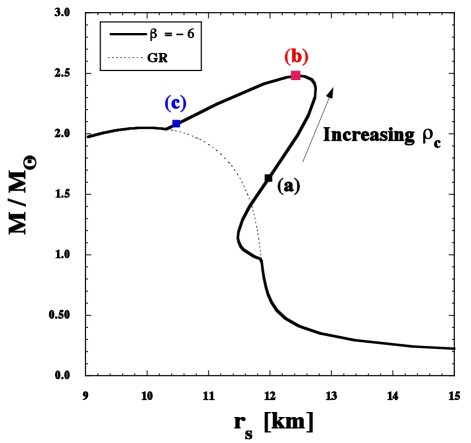
In the left panel of Fig. 1, we plot the mass-radius relation of relativistic star for the nonminimal coupling (5) with . We choose the SLy equation of state inside the star, whose analytic representation is given in Ref. Haensel:2004nu . For each central density , the boundary condition of at is iteratively searched to realize the asymptotic behavior as . For the central density , where , we find that there exists the scalarized branch with besides the GR branch with everywhere. As the central density increases, the mass-radius relation shifts toward the direction of an arrow depicted in Fig. 1.
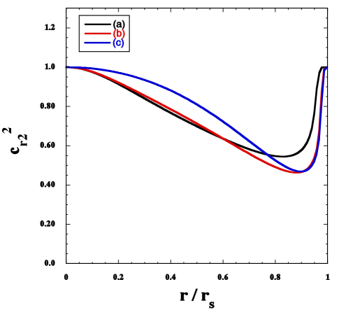
Three cases (a), (b), (c) shown in the left panel of Fig. 1 are in the region where spontaneous scalarization takes place. In the right panel, we plot the propagation speed squared (171) versus for in three different cases (a), (b), (c). For , we find that the matter sound speed squared is subluminal () in the region where spontaneous scalarization occurs. In cases (a), (b), (c) of Fig. 1, we have at the center of NS, respectively. The superluminal propagation of arises for the high central density , but this is the region in which only the GR branch is present. In the right panel of Fig. 1, we can confirm that is subluminal inside the star for the scalarized branch. From Eq. (171) the value of at is equivalent to 1. For increasing from the center, decreases from . Around the surface of star, both and rapidly drop down toward 0, so begins to increase toward the value 1. Besides cases (a), (b), (c), we numerically confirmed that the above subluminal property generally holds throughout the region in which spontaneous scalarization takes place.
From Eq. (174), we have at due to the boundary condition . Provided that , also remains subluminal inside the star and approaches the value 1 toward the surface. Taking the limit in Eqs. (171)-(174), the propagation speed squares , , , and are all equivalent to 1 outside the star. This fact is consistent with the observations of speed of GWs GW170817 .
VII.2 Brans-Dicke theories
Let us proceed to the BD theories given by the action (7), i.e.,
| (177) |
We are considering the coupling , i.e., the BD parameter in the range . Then, it follows that
| (178) |
Therefore, together with the conditions (166), the absence of ghost and Laplacian instabilities is automatically guaranteed. As long as , the propagation speed squares (171)-(174) are subluminal inside the star.
VIII Conclusions
In this paper, we studied the stability of relativistic stars against odd- and even-parity perturbations in scalar-tensor theories given by the action (11). Our interest is the application to hairy NS solutions which are known to exist in theories of spontaneous scalarization and BD theories (see Sec. II). For this purpose, we need to properly deal with the matter sector as a form of the perfect fluid. The Schutz-Sorkin action (12) is suitable for describing the perfect fluid in any background space-time. In Sec. III, we derived covariant equations of motion in scalar-tensor theories (11) with the matter action (12) and applied them to the spherically symmetric and static background.
In Sec. IV, we decomposed the perturbations of gravity, scalar-field, and perfect-fluid sectors into the odd- and even-parity modes. To our knowledge, this type of decomposition including the perfect fluid as a form of the Schutz-Sorkin action was not addressed in the literature. We also defined the matter density perturbation and velocity potential as the quantities related to the number density and four velocity , respectively. The radial direction is singled out on the spherically symmetric and static background, in which case the velocity potential is associated with the and components of .
In Sec. V, we expanded the action (11) up to quadratic order in odd-parity perturbations and obtained the second-order action of the form (81). The perfect fluid does not affect the evolution of GWs in the odd-parity sector. For the multipoles , there is one dynamical degree of freedom with the propagation speed equivalent to that of light. In this case, the ghost is absent under the condition . For , there is no dynamical propagation of odd-parity perturbations.
In Sec. VI, we obtained the second-order action of even-parity perturbations with the multipoles in the form (116) after eliminating some nondynamical perturbations appearing in the Schutz-Sorkin action. We found that there are three propagating degrees of freedom characterized by , , and , where and are given, respectively, by Eqs. (118) and (117). After integrating out all the other nondynamical perturbations, the final second-order action reduces to the form (122) with (123). From the kinetic matrix , we showed that the ghosts are absent under the three conditions (127), (128), and (129). Since we only exploited the relations among coefficients in Eq. (116) applicable to full Horndeski theories, our no-ghost conditions are also valid for Horndeski theories by modifying the coefficients (A.1) in the Appendix to those presented in Ref. Kobayashi:2014wsa .
The matter perturbation associated with the even-parity sector does not propagate along the radial direction by reflecting the property of velocity potential mentioned above. In scalar-tensor theories given by the action (11), the other propagation speed squares are given by Eq. (132). If , which is the case for theories of scalarized relativistic stars discussed in Sec. II, the radial speeds of propagation associated with the perturbations and reduce, respectively, to Eqs. (137) and (138). For , the speed of scalar GWs is different from 1 inside relativistic stars. In the limit , we also derived the three propagation speeds along the angular direction as Eqs. (140)-(142). Again, the perfect fluid affects the angular propagation of scalar GWs.
For the monopole mode () in the even-parity sector, we showed that there are two dynamical perturbations and with the reduced action of the form (146). In this case, the no-ghost conditions are given by Eqs. (153) and (154) with the two radial propagation speeds (156) and (157), so that the latter propagation of scalar-field perturbation is modified by the presence of perfect fluid. For the dipole mode (), the dynamical perturbations correspond to and defined by Eq. (158). In this case, the no-ghost conditions correspond to the limit of those derived for . However, the speed of scalar GWs cannot be recovered in the same limit, so it gives an additional stability condition to those obtained for .
In Sec. VII, we summarized the stability conditions for the absence of ghost and Laplacian instabilities and applied them to the theories with . Provided that the ghost is absent in the odd-parity sector () and that the perfect fluid satisfies the properties and , the sign of defined by Eq. (170) is crucial for the stability of even-parity perturbations. In theories of spontaneous scalarization and BD theories with , we showed that is positive, under which there are neither ghosts nor Laplacian instabilities. Moreover, as long as , the propagation speeds are subluminal inside the star. Indeed, we confirmed this property in theories of spontaneous scalarization with the nonminimal coupling taken by Damour and Esposito-Farese by numerically computing the radial propagation speed squared inside the NS. In such theories, the propagation speeds of GWs in both odd- and even-parity sectors are equivalent to that of light outside the star, so they are consistent with observations of the GW170817 event.
We have thus shown that hairy relativistic stars in scalar-tensor theories given by the action (1) are stable against odd- and even-parity perturbations under mild conditions. The next step is to probe the signature of scalar hairs from observations. In addition to the oscillation of scalar GWs discussed in Ref. Sotani:2005qx , the tidal deformations of NS binaries Flanagan:2007ix ; Damour:2009vw ; Binnington:2009bb ; Hinderer:2009ca may allow one to distinguish between NSs in scalar-tensor theories and in GR. Our general formulation of perturbations around relativistic stars will provide a useful framework for dealing with such problems.
Acknowledgements
R. Kase is supported by the Grant-in-Aid for Young Scientists B of the JSPS No. 17K14297. ST is supported by the Grant-in-Aid for Scientific Research Fund of the JSPS No. 19K03854.
Appendix: Coefficients in the second-order action of even-parity perturbation
References
- (1) B. P. Abbott et al. [LIGO Scientific and Virgo Collaborations], Phys. Rev. Lett. 116, 061102 (2016) [arXiv:1602.03837 [gr-qc]].
- (2) B. P. Abbott et al. [LIGO Scientific and Virgo Collaborations], Phys. Rev. Lett. 119, 161101 (2017) [arXiv:1710.05832 [gr-qc]].
- (3) E. Berti et al., Class. Quant. Grav. 32, 243001 (2015) [arXiv:1501.07274 [gr-qc]].
- (4) L. Barack et al., Class. Quant. Grav. 36, 143001 (2019) [arXiv:1806.05195 [gr-qc]].
- (5) Y. Fujii and K. Maeda, “The scalar-tensor theory of gravitation”, Cambridge University Press (2003).
- (6) A. De Felice and S. Tsujikawa, Living Rev. Rel. 13, 3 (2010) [arXiv:1002.4928 [gr-qc]].
- (7) T. Damour and G. Esposito-Farese, Phys. Rev. Lett. 70, 2220 (1993).
- (8) T. Damour and G. Esposito-Farese, Phys. Rev. D 54, 1474 (1996) [gr-qc/9602056].
- (9) T. Harada, Phys. Rev. D 57, 4802 (1998) [gr-qc/9801049].
- (10) J. Novak, Phys. Rev. D 58, 064019 (1998) [gr-qc/9806022].
- (11) H. O. Silva, C. F. B. Macedo, E. Berti and L. C. B. Crispino, Class. Quant. Grav. 32, 145008 (2015) [arXiv:1411.6286 [gr-qc]].
- (12) P. C. C. Freire et al., Mon. Not. Roy. Astron. Soc. 423, 3328 (2012) [arXiv:1205.1450 [astro-ph.GA]].
- (13) H. Sotani and K. D. Kokkotas, Phys. Rev. D 70, 084026 (2004) [arXiv:gr-qc/0409066 [gr-qc]].
- (14) H. Sotani, Phys. Rev. D 89, 064031 (2014) [arXiv:1402.5699 [astro-ph.HE]].
- (15) H. Sotani, Phys. Rev. D 86, 124036 (2012) [arXiv:1211.6986 [astro-ph.HE]].
- (16) D. D. Doneva, S. S. Yazadjiev, N. Stergioulas and K. D. Kokkotas, Phys. Rev. D 88, 084060 (2013) [arXiv:1309.0605 [gr-qc]].
- (17) D. D. Doneva, S. S. Yazadjiev, K. V. Staykov and K. D. Kokkotas, Phys. Rev. D 90, 104021 (2014) [arXiv:1408.1641 [gr-qc]].
- (18) P. Pani and E. Berti, Phys. Rev. D 90, 024025 (2014) [arXiv:1405.4547 [gr-qc]].
- (19) D. D. Doneva, S. S. Yazadjiev, N. Stergioulas, K. D. Kokkotas and T. M. Athanasiadis, Phys. Rev. D 90, 044004 (2014) [arXiv:1405.6976 [astro-ph.HE]].
- (20) G. Pappas and T. P. Sotiriou, Mon. Not. Roy. Astron. Soc. 453, 2862-2876 (2015) [arXiv:1505.02882 [gr-qc]].
- (21) B. Kleihaus, J. Kunz, S. Mojica and E. Radu, Phys. Rev. D 93, 044047 (2016) [arXiv:1511.05513 [gr-qc]].
- (22) D. D. Doneva and S. S. Yazadjiev, Phys. Rev. Lett. 120, 131103 (2018) [arXiv:1711.01187 [gr-qc]].
- (23) H. O. Silva, J. Sakstein, L. Gualtieri, T. P. Sotiriou and E. Berti, Phys. Rev. Lett. 120, 131104 (2018) [arXiv:1711.02080 [gr-qc]].
- (24) G. Antoniou, A. Bakopoulos and P. Kanti, Phys. Rev. Lett. 120, 131102 (2018) [arXiv:1711.03390 [hep-th]].
- (25) G. Antoniou, A. Bakopoulos and P. Kanti, Phys. Rev. D 97, 084037 (2018) [arXiv:1711.07431 [hep-th]].
- (26) M. Minamitsuji and T. Ikeda, Phys. Rev. D 99, 044017 (2019) [arXiv:1812.03551 [gr-qc]].
- (27) P. V. P. Cunha, C. A. R. Herdeiro and E. Radu, Phys. Rev. Lett. 123, 011101 (2019) [arXiv:1904.09997 [gr-qc]].
- (28) I. Z. Stefanov, S. S. Yazadjiev and M. D. Todorov, Mod. Phys. Lett. A 23, 2915 (2008) [arXiv:0708.4141 [gr-qc]].
- (29) C. A. R. Herdeiro, E. Radu, N. Sanchis-Gual and J. A. Font, Phys. Rev. Lett. 121, 101102 (2018) [arXiv:1806.05190 [gr-qc]].
- (30) P. G. S. Fernandes, C. A. R. Herdeiro, A. M. Pombo, E. Radu and N. Sanchis-Gual, Class. Quant. Grav. 36, no. 13, 134002 (2019) [arXiv:1902.05079 [gr-qc]].
- (31) P. G. S. Fernandes, C. A. R. Herdeiro, A. M. Pombo, E. Radu and N. Sanchis-Gual, Phys. Rev. D 100, 084045 (2019) [arXiv:1908.00037 [gr-qc]].
- (32) T. Ikeda, T. Nakamura and M. Minamitsuji, Phys. Rev. D 100, 104014 (2019) [arXiv:1908.09394 [gr-qc]].
- (33) C. Brans and R. H. Dicke, Phys. Rev. 124, 925 (1961).
- (34) S. Tsujikawa, K. Uddin, S. Mizuno, R. Tavakol and J. Yokoyama, Phys. Rev. D 77, 103009 (2008) [arXiv:0803.1106 [astro-ph]].
- (35) A. Cooney, S. DeDeo and D. Psaltis, Phys. Rev. D 82, 064033 (2010) [arXiv:0910.5480 [astro-ph.HE]].
- (36) A. S. Arapoglu, C. Deliduman and K. Y. Eksi, JCAP 1107, 020 (2011) [arXiv:1003.3179 [gr-qc]].
- (37) M. Orellana, F. Garcia, F. A. Teppa Pannia and G. E. Romero, Gen. Rel. Grav. 45, 771 (2013) [arXiv:1301.5189 [astro-ph.CO]].
- (38) A. V. Astashenok, S. Capozziello and S. D. Odintsov, JCAP 1312, 040 (2013) [arXiv:1309.1978 [gr-qc]].
- (39) S. S. Yazadjiev, D. D. Doneva, K. D. Kokkotas and K. V. Staykov, JCAP 1406, 003 (2014) [arXiv:1402.4469 [gr-qc]].
- (40) M. Aparicio Resco, A. de la Cruz-Dombriz, F. J. Llanes Estrada and V. Zapatero Castrillo, Phys. Dark Univ. 13, 147 (2016) [arXiv:1602.03880 [gr-qc]].
- (41) J. O‘Hanlon, Phys. Rev. Lett. 29, 137 (1972).
- (42) T. Chiba, Phys. Lett. B 575, 1 (2003) [astro-ph/0307338].
- (43) A. A. Starobinsky, Phys. Lett. B 91, 99 (1980).
- (44) A. Ganguly, R. Gannouji, R. Goswami and S. Ray, Phys. Rev. D 89, 064019 (2014) [arXiv:1309.3279 [gr-qc]].
- (45) R. Kase and S. Tsujikawa, JCAP 09, 054 (2019) [arXiv:1906.08954 [gr-qc]].
- (46) A. Dohi, R. Kase, R. Kimura, K. Yamamoto and M. a. Hashimoto, arXiv:2003.12571 [gr-qc].
- (47) A. Maselli, H. O. Silva, M. Minamitsuji and E. Berti, Phys. Rev. D 93, 124056 (2016) [arXiv:1603.04876 [gr-qc]].
- (48) M. Minamitsuji and H. O. Silva, Phys. Rev. D 93, 124041 (2016) [arXiv:1604.07742 [gr-qc]].
- (49) J. Chagoya, G. Niz and G. Tasinato, Class. Quant. Grav. 34, 165002 (2017) [arXiv:1703.09555 [gr-qc]].
- (50) R. Kase, M. Minamitsuji and S. Tsujikawa, Phys. Rev. D 97, 084009 (2018) [arXiv:1711.08713 [gr-qc]].
- (51) J. Chagoya and G. Tasinato, JCAP 08, 006 (2018) [arXiv:1803.07476 [gr-qc]].
- (52) H. Ogawa, T. Kobayashi and K. Koyama, Phys. Rev. D 101, 024026 (2020) [arXiv:1911.01669 [gr-qc]].
- (53) R. Kase, M. Minamitsuji and S. Tsujikawa, arXiv:2001.10701 [gr-qc] (Physical Review D to appear).
- (54) R. J. Scherrer, Phys. Rev. Lett. 93, 011301 (2004) [arXiv:astro-ph/0402316 [astro-ph]].
- (55) D. Giannakis and W. Hu, Phys. Rev. D 72, 063502 (2005) [astro-ph/0501423].
- (56) F. Arroja and M. Sasaki, Phys. Rev. D 81, 107301 (2010) [arXiv:1002.1376 [astro-ph.CO]].
- (57) A. De Felice, S. Mukohyama and S. Tsujikawa, Phys. Rev. D 82, 023524 (2010) [arXiv:1006.0281 [astro-ph.CO]].
- (58) R. Kase and S. Tsujikawa, Phys. Rev. D 90, 044073 (2014) [arXiv:1407.0794 [hep-th]].
- (59) L. Heisenberg, R. Kase and S. Tsujikawa, Phys. Lett. B 760, 617-626 (2016) [arXiv:1605.05565 [hep-th]].
- (60) A. E. Gumrukcuoglu, R. Kimura and K. Koyama, Phys. Rev. D 101, 124021 (2020) [arXiv:2003.11831 [gr-qc]].
- (61) B. F. Schutz and R. Sorkin, Annals Phys. 107, 1 (1977).
- (62) J. D. Brown, Class. Quant. Grav. 10, 1579 (1993) [gr-qc/9304026].
- (63) A. De Felice, J. M. Gerard and T. Suyama, Phys. Rev. D 81, 063527 (2010) [arXiv:0908.3439 [gr-qc]].
- (64) G. W. Horndeski, Int. J. Theor. Phys. 10, 363 (1974).
- (65) C. Deffayet, X. Gao, D. A. Steer and G. Zahariade, Phys. Rev. D 84, 064039 (2011) [arXiv:1103.3260 [hep-th]].
- (66) T. Kobayashi, M. Yamaguchi and J. ’i. Yokoyama, Prog. Theor. Phys. 126, 511 (2011) [arXiv:1105.5723 [hep-th]].
- (67) C. Charmousis, E. J. Copeland, A. Padilla and P. M. Saffin, Phys. Rev. Lett. 108, 051101 (2012) [arXiv:1106.2000 [hep-th]].
- (68) A. De Felice, T. Suyama and T. Tanaka, Phys. Rev. D 83, 104035 (2011) [arXiv:1102.1521 [gr-qc]].
- (69) T. Kobayashi, H. Motohashi and T. Suyama, Phys. Rev. D 85, 084025 (2012) [arXiv:1202.4893 [gr-qc]].
- (70) T. Kobayashi, H. Motohashi and T. Suyama, Phys. Rev. D 89, 084042 (2014) [arXiv:1402.6740 [gr-qc]].
- (71) T. Kobayashi and N. Tanahashi, PTEP 2014, 073E02 (2014) [arXiv:1403.4364 [gr-qc]].
- (72) H. Ogawa, T. Kobayashi and T. Suyama, Phys. Rev. D 93, no.6, 064078 (2016) [arXiv:1510.07400 [gr-qc]].
- (73) E. Babichev, C. Charmousis and A. Lehebel, Class. Quant. Grav. 33, no.15, 154002 (2016) [arXiv:1604.06402 [gr-qc]].
- (74) J. Khoury, M. Trodden and S. S. C. Wong, arXiv:2007.01320 [astro-ph.CO].
- (75) H. Sotani and K. D. Kokkotas, Phys. Rev. D 71, 124038 (2005) [arXiv:gr-qc/0506060 [gr-qc]].
- (76) P. Chen, T. Suyama and J. Yokoyama, Phys. Rev. D 92, 124016 (2015) [arXiv:1508.01384 [gr-qc]].
- (77) S. Morisaki and T. Suyama, Phys. Rev. D 96, 084026 (2017) [arXiv:1707.02809 [gr-qc]].
- (78) T. Regge and J. A. Wheeler, Phys. Rev. 108, 1063 (1957).
- (79) F. J. Zerilli, Phys. Rev. Lett. 24, 737 (1970).
- (80) H. Motohashi and T. Suyama, Phys. Rev. D 84, 084041 (2011) [arXiv:1107.3705 [gr-qc]].
- (81) R. Kase, M. Minamitsuji, S. Tsujikawa and Y. L. Zhang, JCAP 02, 048 (2018) [arXiv:1801.01787 [gr-qc]].
- (82) V. Moncrief, Annals Phys. 88, 323-342 (1974).
- (83) C. O. Lousto and R. H. Price, Phys. Rev. D 55, 2124-2138 (1997) [arXiv:gr-qc/9609012 [gr-qc]].
- (84) P. Haensel and A. Y. Potekhin, Astron. Astrophys. 428, 191 (2004) [astro-ph/0408324].
- (85) E. E. Flanagan and T. Hinderer, Phys. Rev. D 77, 021502 (2008) [arXiv:0709.1915 [astro-ph]].
- (86) T. Damour and A. Nagar, Phys. Rev. D 80 (2009) 084035 [arXiv:0906.0096 [gr-qc]].
- (87) T. Binnington and E. Poisson, Phys. Rev. D 80 (2009) 084018 [arXiv:0906.1366 [gr-qc]].
- (88) T. Hinderer, B. D. Lackey, R. N. Lang and J. S. Read, Phys. Rev. D 81, 123016 (2010) [arXiv:0911.3535 [astro-ph.HE]].