Stability of quasi-particle creation and multiband geometry in fractional Chern insulators under magnetic fields

Similarity of a Bloch band with the LLL is a key to realize an FCI, and there are various models with different degrees of the similarity [9, 10, 11]. In this study, we consider two representative models which have distinct band properties in terms of the quantum geometry. Here, we provide a brief overview of the quantum geometry. The quantum geometric tensor for a single band is given by

where $\alpha,\beta\in\{x,y\}$ and $\bm{k}$ is a wave vector in the Brillouin zone. $A$ is the area of the Brillouin zone. $\ket{u_{\bm{k}}}$ is the cell-periodic function for the band which we focus on, and ${\mathcal{P}}(\bm{k})=\ket{u_{\bm{k}}}\bra{u_{\bm{k}}}$ is the corresponding projection operator. $g(\bm{k})$ and $\mathcal{F}(\bm{k})$ are Fubini-Study metric and Berry curvature, respectively. They are given as real and imaginary parts of the quantum geometric tensor, and known to satisfy the following inequality,

for arbitrary $\bm{k}$ in the Brillouin zone. It is known that a holomorphic wavefunction in the momentum space is given by a single-particle eigenfunction which saturates the inequality and has a positive-definite Berry curvature [9, 10]. Such a holomorphic single-particle wavefunction can lead to the FCI in the presence of short-range interactions. Hence, this geometric condition is called the ideal condition and the corresponding wavefunctions are known as generalization of the LLL. Moreover, a single-particle band satisfying the ideal condition is classified as a vortexable band from a perspective of the vortexability which extends the ideal condition to a larger family [14, 15], and it has been suggested that these frameworks can also apply to multiband systems [16, 17, 18]. The mutliband quantum geometry will be discussed in Sec. V.

We introduce two models to understand the quasi-particle creation and the stability of the FCIs against magnetic fields: the Kapit-Mueller model [23, 24] and the checkerboard model [40]. Both models have flat bands with the Chern number $|C_{\text{s}}|=|(1/2\pi A)\int d^{2}k\mathcal{F}_{xy}|=1$ and realize the FCIs in the absence of magnetic fields, but they have different quantum geometries. In presence of interactions, FCI states are driven in these models. In this study, we consider spinless fermions with the nearest neighbor interaction

where $U$ is the strength of the interaction and $\langle\dots\rangle$ means the nearest-neighbor sites. The operator $n_{j}$ is the number operator $n_{j}=c_{j}^{\dagger}c_{j}$ on site $j$, where $c_{j}$ is the fermion annihilation operator. We use the periodic boundary condition throughout this study.

The Hamiltonian of the Kapit-Mueller model under a magnetic field is,

where $z_{k}=x_{k}+iy_{k}$ is the lattice complex coordinate for the site $k$ and $z=z_{j}-z_{k}=x+iy$. $\phi_{0}$ is a model parameter which is distinguished from the applied flux and chosen to be $\phi_{0}=1/3$. For this parameter, there are three energy bands in the absence of the magnetic field, and the lowest energy band is exactly flat and has a Chern number $C_{s}=1$. In addition, it satisfies the ideal condition and thus the single-particle Bloch function of this band is a holomorphic function. $\phi$ is the applied flux per plaquette, and there is no distinction between the flux and the magnetic field in this study since the lattice constant is the length unit. Note that, since $\phi$ is not included in the Gaussian factor in the hopping integral $J(z_{j},z_{k})$, the Poisson summation rule [23, 41] for hopping integrals does not hold at $\phi\neq 0$ and the ideal condition is not necessarily satisfied under the magnetic field. Nevertheless, deviation from the ideal condition is small as will be discussed later in Sec. V. $G_{jk}$ is the phase factor corresponding to the magnetic field $\phi$ in addition to the model parameter $\phi_{0}=1/3$. We use the string gauge [42, 43, 44, 45],

where $L_{x},L_{y}$ are the linear system sizes in each direction. $\delta_{x}=\pm 1$ for the hopping between $x=0$ and $x=L_{x}-1$ and $\delta_{x}=0$ otherwise. In this gauge, one can describe the flux per square plaquette $\phi=N_{\phi}/N_{s}$ with the number of the sites $N_{s}$, where $N_{\phi}$ is the number of the flux quanta applied to the entire system. The fermion filling for the lowest energy band at $\phi=0$ is $\nu=N/N_{\text{orb}}=1/3$, where $N$ is the number of the fermions and $N_{\text{orb}}$ is the number of the single-particle states in the lowest energy band. $N_{\text{orb}}=N_{s}/3$ at $\phi=0$ and it changes as $\phi$ is introduced. The ground state at $\phi=0$ is the $\nu=1/3$ Laughlin state on the lowest energy band.

The Hamiltonian of the checkerboard model [40] is

The NN, NNN and NNNN hopping mean the nearest-neighbor, the second nearest-neighbor and the third nearest-neighbor hopping respectively. In this study, we set $t=1,\psi_{jk}=\pm\pi/4$, whose sign is determined by the direction of the arrow in Fig.1(b), and $t^{\prime}_{jk}=t_{1},t_{2}$ which is identified by choosing a bipartite site and $t_{1}=-t_{2}=1/(2+\sqrt{2})$. In addition, we set $t^{\prime\prime}=1/(2+2\sqrt{2})$ to realize a nearly flat Chern band with $C_{\text{s}}=-1$ at zero magnetic field, $G_{jk}(\phi=0)=1$. This system exhibits the $\nu=1/3$ Laughlin state on the lowest energy band  [46]. However, because this is a two-band model, its Berry curvature must have at least one zero point in the Brillouin zone, and the trace condition does not hold exactly  [47, 13]. Therefore, the checkerboard model does not satisfy the ideal condition in contrast to the Kapit-Mueller model. The phase factor $G_{jk}(\phi)$ describes the Peierls phase. The concrete expression of $G_{jk}$ for the checkerboard model is essentially the same as that in the Kapit-Mueller model (Eq. (6)) [45]. The fermion filling in the absence of the magnetic field is $\nu=N/N_{\text{orb}}=1/3$, where $N_{\text{orb}}=N_{s}/2$ at $\phi=0$.

In this section, we study the FCI with use of the exact diagonalization. First, we briefly explain how to characterize an FCI state within the exact diagonalization. To examine stability of the FCI states against magnetic fields, we apply one flux quantum $N_{\phi}=\pm 1$ uniformly over the entire system and discuss quasi-particles induced by the magnetic field based on the “counting-rule” on the energy spectra [1, 51, 52]. Previous works examined quasi-hole and quasi-electron creations in FCIs at $\phi=0$ based on the counting-rule, when the number of unit cells is increased or decreased [37, 38, 39]. When the system size is changed with a fixed number $N$ of the fermions, the number of the nearly degenerate single-particle states $N_{\text{orb}}$ and the filling $\nu=N/N_{\text{orb}}$ varies, while the single-particle band structure itself is unchanged. Instead of varying the system size, a change in the number of the single-particle orbits can be induced by the magnetic field according to the Streda’s formula, $N_{\text{orb}}\to N_{\text{orb}}+C_{s}N_{\phi}$. In contrast to the system-size induced change of $N_{\text{orb}}$, the system does not keep the (magnetic) translation symmetry under the additional one flux quantum $N_{\phi}=\pm 1$ [44]. However, one can still regard the nearly degenerate single-particle orbits as a nearly flat band and discuss the stability of the FCI in a manner similar to those in the previous studies at $\phi=0$.

Since the single-particle Chern number is $|C_{s}|=1$ in the present models, a single flux quantum leads to the change $N_{\text{orb}}\to N_{\text{orb}}\pm 1$. This gives rise to creation of one quasi-hole or quasi-electron with the fractional charge $|e^{*}|=1/3$. In case of the quasi-hole creation, the ground state degeneracy $\#_{\text{qh}}$ under the magnetic field obeys the counting rule given by  [1]

where $N_{\text{orb}}$ is the number of the low energy single-particle states in the presence of the magnetic field. For quasi-electron creation, no simple formula for the ground state degeneracy $\#_{\text{qe}}$ is known, but we can verify the counting rule of the quasi-electrons by referring to energy spectra of the corresponding FQHE states. More precisely, we calculate $\#_{\text{qe}}$ for the LLL in the electron gas model and also for fermions in the Kapit-Mueller model with the Poisson summation rule which is a lattice realization of the LLL [23, 41]. We numerically find that $\#_{\text{qe}}=11$ for $(N=4,N_{\text{orb}}=11)$, $\#_{\text{qe}}=14$ for $(N=5,N_{\text{orb}}=14)$, and $\#_{\text{qe}}=17$ for $(N=6,N_{\text{orb}}=17)$.

The quasi-particles created by the uniform magnetic field are extended over the entire system. They can be spatially localized in the presence of an additional pinning potential $V_{p}$ which couples with the quasi-particle charge [35]. To this end, we first perform the exact diagonalization to obtain low energy states $\ket{\Psi_{1}},\ket{\Psi_{2}},\cdots,\ket{\Psi_{N_{\text{cut}}}}$ without the pinning potential [37, 38], where $N_{\text{cut}}=\#_{\text{qh}}$ or $\#_{\text{qe}}$ is a cut-off for the low energy states. Then, we take $V_{p}$ into account within this low energy sector by diagonalizing the projected Hamiltonian with the pinning potential,

where $H$ is either $H_{\text{KM}}$ or $H_{\text{CB}}$. $P$ is the projection onto the low energy states $\{\ket{\Psi_{n}}\}_{n=1}^{N_{\text{cut}}}$ and $j_{0}$ is the position of the pinning potential. The projection enables us to efficiently focus on the low energy sector and also greatly reduces computational costs for the analysis of the pinning potential [37, 38]. When the quasi-particle created by $\phi\neq 0$ is localized by the pinning potential, it does not contribute to the Hall conductance. Correspondingly, the ground state degeneracy of $\tilde{H}$ will be three fold for the present $\nu=1/3$ system. In this sense, the ground states of $\tilde{H}$ belong to the same FCI phase of $H$ at $\phi=0$. However, the quasi-particle creation can be unstable and a magnetic field may destabilize the underlying FCI state. In this case, the counting rule does not hold and the ground states of $\tilde{H}$ are no longer FCIs.

We can further characterize the ground states of $\tilde{H}$ as FCIs by calculating the many-body Chern number $C$, with use of the Fukui-Hatsugai-Suzuki’s method [53, 54, 55]. The many-body Chern number $C$ is defined as

where $F(\vec{\theta})=\partialderivative{A_{y}}{\theta_{x}}-\partialderivative{A_{x}}{\theta_{y}}$, $A_{\mu}(\vec{\theta})=i\Phi^{{\dagger}}\partialderivative{\Phi}{\theta_{\mu}}$, and $\Phi(\vec{\theta})=(\ket{\Psi_{1}(\vec{\theta})},\dots,\ket{\Psi_{q}(\vec{\theta})})^{T}$ is the ground state multiplet with $q=3$. $\vec{\theta}=(\theta_{x},\theta_{y})$ represents a twisting phase for which $c_{n_{x}+L_{x},n_{y}}=e^{i\theta_{x}}c_{n_{x},n_{y}}$ and $c_{n_{x},n_{y}+L_{y}}=e^{i\theta_{y}}c_{n_{x},n_{y}}$. We divide the parameter space $\{(\theta_{x},\theta_{y})\}=[0,2\pi]\times[0,2\pi]$ into $L_{\theta}\times L_{\theta}$ discrete points with $L_{\theta}=20$, which is large enough to accurately compute $C$. Note that the Fukui-Hatsugai-Suzuki’s method gives a quantized value of $C$ by construction even for a gapless state in a finite size system, and it does not give any physical implications in such a case.

To supplement our argument, we also examine the one-plaquette Chern number defined as

in the discretized parameter space. It is known that, in a gapped system, $\mathcal{C}(\vec{\theta})$ is approximately uniform in the parameter space and it is close to $C$ given by Eq. (13) [55, 56]. To verify the uniformity, we examine the variance of $\mathcal{C}(\theta_{x},\theta_{y})$,

The variance is exponentially small if the ground states are FCIs, while it can be large for gapless states. In this way, we can identify FCI states within the exact diagonalization for small system sizes. It turns out that, even if the ground state of $\tilde{H}$ is an FCI, $\mathcal{V}[\mathcal{C}]$ diverges when we use $N_{\text{cut}}<\#_{\text{qh}},\#_{\text{qe}}$. When $N_{\text{cut}}=\#_{\text{qh}},\#_{\text{qe}}$, the variance $\mathcal{V}[\mathcal{C}]$ is suppressed in the FCI phase.

In this study, we consider the systems with the number of the fermions $N=4\sim 6$. This is relatively small compared to those in the previous studies where quasi-particles are created by the increase of the system sizes [1, 37, 38, 39]. Technically, one flux quantum breaks the (magnetic) translation symmetry and the size of the Hilbert space cannot be reduced by the translation symmetry [44]. However, it turns that we can discuss physical properties of the systems with $N=4\sim 6$ by carefully paying attention to finite size effects as will be discussed in the following sections. Furthermore, we have confirmed that quasi-particles are stably created by the increase of the system sizes for $N=4,5$ in consistent with the previous studies [37, 38, 39]. This implies that finite size effects are small for these system sizes.

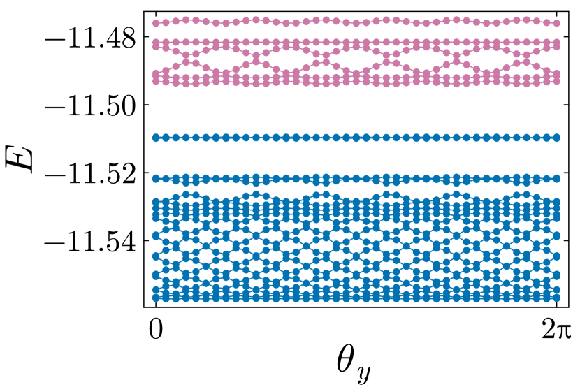
We first discuss the quasi-hole creation in the Kapit-Mueller model. In Fig. 3, we show spectral-flow for the Kapit-Mueller model with one additional positive flux quantum $N_{\phi}=1$. The counting-rule for the quasi-holes is $\#_{\text{qh}}=13$ for the present system with $N=4,N_{s}/3=12,C_{\text{s}}N_{\phi}=1$, and correspondingly the lowest 13 energy levels are shown in blue in Fig. 3(a). There exists a clear energy gap between the set of the blue curves and others, which means that the counting-rule is satisfied. Figure 3(b) represents spectral flow for the system with the pinning potential $V_{p}=1.0$, where the blue curves represent the three lowest energy states. Now these three fold quasi-degenerate states are well separated from other states, and they are expected to exhibit the fractionally quantized Hall conductance as mentioned in the previous section [35]. Indeed, we find that the many-body Chern number for the three fold quasi-degenerate ground states for $V_{p}=1.0$ is $C=1$ corresponding to the $\nu=1/3$ FQHE. In addition, the one-plaquette Chern number $\mathcal{C}(\vec{\theta})$ is nearly flat in the parameter space as shown in Fig. 4(a). These results are fully consistent with the qualitative discussions in the previous section. Namely, the quasi-holes obeying the counting rule are created by the magnetic field and then get localized by the pinning potential, which consequently leads to the FCI ground state for $\phi\neq 0$ and $V_{p}\neq 0$. Qualitatively same results are obtained for other values of the interaction strength, $U=1.0\sim 8.0$. The FCI state is unstable and a non-FCI state is realized only around the non-interacting limit $U=0$.

Next we consider the quasi-electron creation in the presence of one additional negative flux quantum $N_{\phi}=-1$. Spectral flow with no pinning potential at $N=4,U=1.0$ is shown in Fig. 3(c). As mentioned in the previous section, the counting rule for the quasi-electrons is $\#_{\text{qe}}=11$. It is found that there are 11 fold quasi-degeneracy for the present Kapit-Mueller model, and thus the quasi-electrons are stably created by the mangnetic field. Similarly to the quasi-hole case, spectral flow with the pinning potential (Fig. 3(d)) also shows the three fold quasi-degenerate ground states which are separated from other excited states with a gap. Note that, in the quasi-electron case, a negative pinning potential $V_{p}=-1.0$ is necessary to localize the quasi-electron, since it has a positive fractional charge as opposed to the quasi-holes. The many-body Chern number of the three fold quasi-degenerate ground states is found to be $C=1$, and the one-plaquette Chern number is uniform as shown in Fig. 4 (b). Similar results are obtained for $U=1.0\sim 8.0$.

Finally, we show the variance $\mathcal{V}[\mathcal{C}]$ for various interaction strength and the flux $N_{\phi}=0,\pm 1(\phi=0,\pm 0.028)$ in Fig. 4 (c). The variance is very small and therefore the FCI ground states of $\tilde{H}$ are stable even for the small system with $N=4$. For larger systems, finite size effects will be further suppressed and one flux quantum corresponds to smaller magnetic fields. Therefore, the ground states of $\tilde{H}$ for such systems will also be stable FCIs. We have numerically confirmed that this is indeed the case for $N=5$. Based on these observations, we expect the quantum phase diagram of the Kapit-Mueller model shown in Fig. 2(a) in the previous section. The phase diagram has been extrapolated to the region $|\phi|>0.03$ based on the analyses of the quantum geometry under magnetic fields in Sec. V.

We present numerical results of the spectral flow for the quasi-hole creation in the checkerboard model at $N=6,U=1.0$ in Fig. 5(a). The blue curves in Fig.5(a) represent the energy levels expected from the counting rule, $\#_{\text{qh}}=19$ for $N=6,N_{s}/2=18,C_{s}N_{\phi}=1$. However, at $U=1.0$, there is no clear energy gap between the blue curves and others, and it is difficult to identify the ground state sector in contrast to the Kapit-Mueller model in the previous section. Consequently, there are no clear three fold quasi-degenerate ground states with the pinning potential as shown in Fig. 5(b). Note that the pinning potential is sufficiently large $V_{p}=10$ so that density distribution is well localized around the site $j_{0}$, and we have confirmed the absence of the quasi-degeneracy for other values of the pinning potential. This implies that quasi-holes are not created and the underlying FCI state is no longer stable in the presence of the magnetic field. Indeed, the one-plaquette Chern number for the three lowest energy states in Fig. 5(b) diverges and has large fluctuations (Fig. 6(a)). Since the one-plaquette Chern number is nearly flat in the $\theta$-space in a general gapped system in the thermodynamic limit [55, 56], the strong divergence implies that the present system with $U=1$ does not have the three fold topological quasi-degeneracy. Therefore, the ground state is a non-FCI state.

However, as we increase the interaction strength from $U=1.0$ to $U=2.0,3.0$, an energy gap develops in the spectral flow at $V_{p}=0$ and the low energy 19 states become separated from others as seen in Fig. 5(c),(e). Furthermore, in the presence of the pinning potential, we find that there exists a clear gap between the three lowest energy levels and other excitations. The many-body Chern number for these three fold quasi-degenerate states is $C=-1$ and the variance $\mathcal{V}[\mathcal{C}]$ for $U=2.0\sim 3.0$ is suppressed as shown in Figs. 6 and  7. These results suggest that there is a quantum phase transition from the non-FCI state to the stable FCI state as $U$ increases. The phase transition point is located around $U=2.0$, where the diverging behaviors of the variance $\mathcal{V}[\mathcal{C}]$ get suppressed and it becomes rather flat as seen in Fig. 7(b). To be more precise, a quantum phase transition is well defined only in the thermodynamic limit. In a thermodynamically large system, the number of the fluxes is $|N_{\phi}|\gg 1$ for a fixed magnetic field $\phi$ and there will be $|N_{\phi}|$ quasi-particles localized by a pinning potential corresponding to disorder. We have simply assumed that effects of interactions between the pinned quasi-particles are negligible. This enables us to discuss the phase transition based on the exact diagonalization for the small system with $|N_{\phi}|=1$.

Similar phase transitions are found for the systems with different numbers of the fermions, $N=4,5$. The applied flux per plaquette is $\phi=-1/N_{s}\simeq-0.042$ for $N=4$ and $\phi\simeq-0.033$ for $N=5$, which enables us to discuss magnetic field dependence of the quantum phase transition. Similarly to the $N=6$ case, as $U$ increases, energy gaps develop between the $\#_{\text{qh}}$ lowest energy states and other states at $V_{p}=0$, and also between the three lowest energies and excited states for $V_{p}\neq 0$ (see Appendix B for details). We find that the strength of the interactions $U_{c}$ required to stabilize the FCI increases as $N$ decreases. Besides, the variance of the Chern number is large for small interactions as seen in Fig. 7(b). Based on these numerical results, we suppose that the phase transition occurs at $U_{c}=2.0\sim 3.0$ for $N=5$ and $U_{c}=4.0\sim 5.0$ for $N=4$. This in turn implies that the critical interaction $U_{c}$ increases as the negative magnetic field increases. There would be some finite size effects for smaller system sizes, but we can confirm that it is not relevant in the present system. First, when the system size is changed, quasi-holes are stably created for $N=5,U=1.0$ at $\phi=0$ (Appendix A), which means that the absence of the FCI state for $N=5,U=1.0$ at $\phi\simeq-0.033$ is due to the magnetic field. Second, as will be discussed in the following, the FCI state becomes stable when the direction of the magnetic field is changed, $\phi\to-\phi$. Therefore, the stability of the FCI state is dominated by the magnetic field.

In contrast to the quasi-hole case, creation of the quasi-electrons is stable even for small interactions. As shown in Fig. 8 and Fig. 15 in Appendix B, the counting rule derived from the numerical results for the FQHE and the three fold quasi-degeneracy are realized for $N=4,5,6$ at $U\approx 1.0$. Moreover, the many-body Chern number $C=-1$ is robust even at the small interaction $U=1.0$ for all $N=4,5,6$. Note that the variance ${\mathcal{V}}[C]$ is slightly large at $U=1.0$ for $N=4$ and $5$, but this may be due to finite size effects and ${\mathcal{V}}[C]$ is quickly suppressed for larger $U$. Thus, the stable FCI region is extended over a wide range of interaction strength and magnetic fields for the quasi-electron creation.

In Fig. 9, we summarize the numerical results of the variance ${\mathcal{V}}[C]$ as an indicator for the FCI state. The many-body Chern number for the three fold quasi-degenerate ground states with $V_{p}\neq 0$ is $C=-1$ and it has small fluctuation ${\mathcal{V}}[C]$ in the FCI state, while the Chern number is not well defined and the variance diverges in the non-FCI state. The flux $|\phi|=1/N_{s}\simeq 0.042,0.033,0.028$ corresponds to the different numbers of the fermions, $N=4,5,6$, respectively. We see that the creation of the quasi-particles and the underlying FCI state are stable for a wide range of the parameters, while the non-FCI state is realized around the non-interaction region $U=0$ and under negative fluxes even with moderate interactions. Based on these results, we obtain the expected phase diagram Fig. 2(b) in Sec. III. It is difficult to clarify details of the non-FCI state within the present calculations, and further discussions are left for a future study.

References

- Regnault and Bernevig [2011] N. Regnault and B. A. Bernevig, Fractional chern insulator, Phys. Rev. X 1, 021014 (2011).
- Neupert et al. [2011] T. Neupert, L. Santos, C. Chamon, and C. Mudry, Fractional quantum hall states at zero magnetic field, Phys. Rev. Lett. 106, 236804 (2011).
- Wu et al. [2012] Y.-L. Wu, B. A. Bernevig, and N. Regnault, Zoology of fractional chern insulators, Phys. Rev. B 85, 075116 (2012).
- Grushin et al. [2015] A. G. Grushin, J. Motruk, M. P. Zaletel, and F. Pollmann, Characterization and stability of a fermionic fractional chern insulator, Phys. Rev. B 91, 035136 (2015).
- Tang et al. [2011] E. Tang, J.-W. Mei, and X.-G. Wen, High-temperature fractional quantum hall states, Phys. Rev. Lett. 106, 236802 (2011).
- Parameswaran et al. [2013] S. A. Parameswaran, R. Roy, and S. L. Sondhi, Fractional quantum hall physics in topological flat bands, Comptes Rendus Physique 14, 816 (2013), topological insulators / Isolants topologiques.
- BERGHOLTZ and LIU [2013] E. J. BERGHOLTZ and Z. LIU, Topological flat band models and fractional chern insulators, International Journal of Modern Physics B 27, 1330017 (2013), https://doi.org/10.1142/S021797921330017X .
- Liu and Bergholtz [2024] Z. Liu and E. J. Bergholtz, Recent developments in fractional chern insulators, in Encyclopedia of Condensed Matter Physics (Second Edition), edited by T. Chakraborty (Academic Press, Oxford, 2024) second edition ed., pp. 515–538.
- Wang et al. [2021] J. Wang, J. Cano, A. J. Millis, Z. Liu, and B. Yang, Exact landau level description of geometry and interaction in a flatband, Phys. Rev. Lett. 127, 246403 (2021).
- Wang et al. [2023] J. Wang, S. Klevtsov, and Z. Liu, Origin of model fractional chern insulators in all topological ideal flatbands: Explicit color-entangled wave function and exact density algebra, Phys. Rev. Res. 5, 023167 (2023).
- Roy [2014] R. Roy, Band geometry of fractional topological insulators, Phys. Rev. B 90, 165139 (2014).
- Ozawa and Mera [2021] T. Ozawa and B. Mera, Relations between topology and the quantum metric for chern insulators, Phys. Rev. B 104, 045103 (2021).
- Lee et al. [2017] C. H. Lee, M. Claassen, and R. Thomale, Band structure engineering of ideal fractional chern insulators, Phys. Rev. B 96, 165150 (2017).
- Ledwith et al. [2023] P. J. Ledwith, A. Vishwanath, and D. E. Parker, Vortexability: A unifying criterion for ideal fractional chern insulators, Phys. Rev. B 108, 205144 (2023).
- Okuma [2024] N. Okuma, Constructing vortex functions and basis states of chern insulators: ideal condition, inequality from index theorem, and coherent-like states on von neumann lattice (2024), arXiv:2405.11796 [cond-mat.mes-hall] .
- Parker et al. [2021] D. Parker, P. Ledwith, E. Khalaf, T. Soejima, J. Hauschild, Y. Xie, A. Pierce, M. P. Zaletel, A. Yacoby, and A. Vishwanath, Field-tuned and zero-field fractional chern insulators in magic angle graphene (2021), arXiv:2112.13837 [cond-mat.str-el] .
- Fujimoto et al. [2024] M. Fujimoto, D. E. Parker, J. Dong, E. Khalaf, A. Vishwanath, and P. Ledwith, Higher vortexability: zero field realization of higher landau levels (2024), arXiv:2403.00856 [cond-mat.mes-hall] .
- Liu et al. [2024] Z. Liu, B. Mera, M. Fujimoto, T. Ozawa, and J. Wang, Theory of generalized landau levels and implication for non-abelian states (2024), arXiv:2405.14479 [cond-mat.mes-hall] .
- Schoonderwoerd et al. [2022] L. Schoonderwoerd, F. Pollmann, and G. Möller, Interaction-driven plateau transition between integer and fractional chern insulators (2022), arXiv:1908.00988 [cond-mat.str-el] .
- Luo et al. [2021] W.-W. Luo, A.-L. He, Y.-F. Wang, Y. Zhou, and C.-D. Gong, Bosonic fractional chern insulating state at integer fillings in a multiband system, Phys. Rev. B 104, 115126 (2021).
- Ma et al. [2024] J.-Z. Ma, R.-Z. Huang, G.-Y. Zhu, J.-Y. Chen, and D.-X. Yao, Fractional chern insulator candidate on a twisted bilayer checkerboard lattice, Phys. Rev. B 110, 165142 (2024).
- Ledwith et al. [2020] P. J. Ledwith, G. Tarnopolsky, E. Khalaf, and A. Vishwanath, Fractional chern insulator states in twisted bilayer graphene: An analytical approach, Phys. Rev. Res. 2, 023237 (2020).
- Kapit and Mueller [2010] E. Kapit and E. Mueller, Exact parent hamiltonian for the quantum hall states in a lattice, Phys. Rev. Lett. 105, 215303 (2010).
- Varjas et al. [2022] D. Varjas, A. Abouelkomsan, K. Yang, and E. J. Bergholtz, Topological lattice models with constant Berry curvature, SciPost Phys. 12, 118 (2022).
- Ledwith et al. [2022] P. J. Ledwith, A. Vishwanath, and E. Khalaf, Family of ideal chern flatbands with arbitrary chern number in chiral twisted graphene multilayers, Phys. Rev. Lett. 128, 176404 (2022).
- Andrews et al. [2024] B. Andrews, M. Raja, N. Mishra, M. P. Zaletel, and R. Roy, Stability of fractional chern insulators with a non-landau level continuum limit, Phys. Rev. B 109, 245111 (2024).
- Shavit and Oreg [2024] G. Shavit and Y. Oreg, Quantum geometry and stabilization of fractional chern insulators far from the ideal limit, Phys. Rev. Lett. 133, 156504 (2024).
- Spanton et al. [2018] E. M. Spanton, A. A. Zibrov, H. Zhou, T. Taniguchi, K. Watanabe, M. P. Zaletel, and A. F. Young, Observation of fractional chern insulators in a van der waals heterostructure, Science 360, 62 (2018), https://www.science.org/doi/pdf/10.1126/science.aan8458 .
- Xie et al. [2021] Y. Xie, A. T. Pierce, J. M. Park, D. E. Parker, E. Khalaf, P. Ledwith, Y. Cao, S. H. Lee, S. Chen, P. R. Forrester, K. Watanabe, T. Taniguchi, A. Vishwanath, P. Jarillo-Herrero, and A. Yacoby, Fractional chern insulators in magic-angle twisted bilayer graphene, Nature 600, 439 (2021).
- Cai et al. [2023] J. Cai, E. Anderson, C. Wang, X. Zhang, X. Liu, W. Holtzmann, Y. Zhang, F. Fan, T. Taniguchi, K. Watanabe, Y. Ran, T. Cao, L. Fu, D. Xiao, W. Yao, and X. Xu, Signatures of fractional quantum anomalous hall states in twisted mote2, Nature 622, 63 (2023).
- Zeng et al. [2023] Y. Zeng, Z. Xia, K. Kang, J. Zhu, P. Knüppel, C. Vaswani, K. Watanabe, T. Taniguchi, K. F. Mak, and J. Shan, Thermodynamic evidence of fractional chern insulator in moiré mote2, Nature 622, 69 (2023).
- Park et al. [2023] H. Park, J. Cai, E. Anderson, Y. Zhang, J. Zhu, X. Liu, C. Wang, W. Holtzmann, C. Hu, Z. Liu, T. Taniguchi, K. Watanabe, J.-H. Chu, T. Cao, L. Fu, W. Yao, C.-Z. Chang, D. Cobden, D. Xiao, and X. Xu, Observation of fractionally quantized anomalous hall effect, Nature 622, 74 (2023).
- Xu et al. [2023] F. Xu, Z. Sun, T. Jia, C. Liu, C. Xu, C. Li, Y. Gu, K. Watanabe, T. Taniguchi, B. Tong, J. Jia, Z. Shi, S. Jiang, Y. Zhang, X. Liu, and T. Li, Observation of integer and fractional quantum anomalous hall effects in twisted bilayer , Phys. Rev. X 13, 031037 (2023).
- Lu et al. [2024] Z. Lu, T. Han, Y. Yao, A. P. Reddy, J. Yang, J. Seo, K. Watanabe, T. Taniguchi, L. Fu, and L. Ju, Fractional quantum anomalous hall effect in multilayer graphene, Nature 626, 759 (2024).
- Yoshioka [2002] D. Yoshioka, The Quantum Hall Effect, Physics and astronomy online library (Springer, 2002).
- Nayak et al. [2008] C. Nayak, S. H. Simon, A. Stern, M. Freedman, and S. Das Sarma, Non-abelian anyons and topological quantum computation, Rev. Mod. Phys. 80, 1083 (2008).
- Liu et al. [2015] Z. Liu, R. N. Bhatt, and N. Regnault, Characterization of quasiholes in fractional chern insulators, Phys. Rev. B 91, 045126 (2015).
- Jaworowski et al. [2019] B. d. z. Jaworowski, N. Regnault, and Z. Liu, Characterization of quasiholes in two-component fractional quantum hall states and fractional chern insulators in =2 flat bands, Phys. Rev. B 99, 045136 (2019).
- Liu et al. [2013] T. Liu, C. Repellin, B. A. Bernevig, and N. Regnault, Fractional chern insulators beyond laughlin states, Phys. Rev. B 87, 205136 (2013).
- Sun et al. [2011] K. Sun, Z. Gu, H. Katsura, and S. Das Sarma, Nearly flatbands with nontrivial topology, Phys. Rev. Lett. 106, 236803 (2011).
- Shen et al. [2025] X. Shen, G. Ji, J. Zhang, D. E. Palomino, B. Mera, T. Ozawa, and J. Wang, Exact parent hamiltonians for all landau level states in a half-flux lattice (2025), arXiv:2501.09742 [cond-mat.mes-hall] .
- Hatsugai et al. [1999] Y. Hatsugai, K. Ishibashi, and Y. Morita, Sum rule of hall conductance in a random quantum phase transition, Phys. Rev. Lett. 83, 2246 (1999).
- Kudo et al. [2017] K. Kudo, T. Kariyado, and Y. Hatsugai, Many-body chern numbers of = 1/3 and 1/2 states on various lattices, Journal of the Physical Society of Japan 86, 103701 (2017).
- Tada [2021] Y. Tada, Lieb-schultz-mattis theorem in higher dimensions from approximate magnetic translation symmetry, Phys. Rev. Lett. 127, 237204 (2021).
- [45] Y. Tada and M. Oshikawa, In preparation.
- Sheng et al. [2011] D. N. Sheng, Z.-C. Gu, K. Sun, and L. Sheng, Fractional quantum hall effect in the absence of landau levels, Nature Communications 2, 389 (2011).
- Mera and Ozawa [2021] B. Mera and T. Ozawa, Kähler geometry and chern insulators: Relations between topology and the quantum metric, Phys. Rev. B 104, 045104 (2021).
- Streda [1982] P. Streda, Theory of quantised hall conductivity in two dimensions, Journal of Physics C: Solid State Physics 15, L717 (1982).
- Streda and Smrcka [1983] P. Streda and L. Smrcka, Thermodynamic derivation of the hall current and the thermopower in quantising magnetic field, Journal of Physics C: Solid State Physics 16, L895 (1983).
- Widom [1982] A. Widom, Thermodynamic derivation of the hall effect current, Physics Letters A 90, 474 (1982).
- Bernevig and Haldane [2008] B. A. Bernevig and F. D. M. Haldane, Model fractional quantum hall states and jack polynomials, Phys. Rev. Lett. 100, 246802 (2008).
- Bernevig and Regnault [2012] B. A. Bernevig and N. Regnault, Emergent many-body translational symmetries of abelian and non-abelian fractionally filled topological insulators, Phys. Rev. B 85, 075128 (2012).
- Niu et al. [1985] Q. Niu, D. J. Thouless, and Y.-S. Wu, Quantized hall conductance as a topological invariant, Phys. Rev. B 31, 3372 (1985).
- Fukui et al. [2005] T. Fukui, Y. Hatsugai, and H. Suzuki, Chern numbers in discretized brillouin zone: Efficient method of computing (spin) hall conductances, Journal of the Physical Society of Japan 74, 1674 (2005).
- Kudo et al. [2019] K. Kudo, H. Watanabe, T. Kariyado, and Y. Hatsugai, Many-body chern number without integration, Phys. Rev. Lett. 122, 146601 (2019).
- Koma [2015] T. Koma, Topological current in fractional chern insulators (2015), arXiv:1504.01243 [math-ph] .
- Girvin et al. [1986] S. M. Girvin, A. H. MacDonald, and P. M. Platzman, Magneto-roton theory of collective excitations in the fractional quantum hall effect, Phys. Rev. B 33, 2481 (1986).