Stability of Linear Set-Membership Filters With Respect to Initial Conditions: An Observation-Information Perspective
Abstract
The issue of filter stability with respect to (w.r.t.) the initial condition refers to the unreliable filtering process caused by improper prior information of the initial state. This paper focuses on analyzing and resolving the stability issue w.r.t. the initial condition of the classical Set-Membership Filters (SMFs) for linear time-invariance systems, which has not yet been well understood in the literature. To this end, we propose a new concept – the Observation-Information Tower (OIT), which describes how the measurements affect the estimate in a set-intersection manner without relying on the initial condition. The proposed OIT enables a rigorous stability analysis, a new SMFing framework, as well as an efficient filtering algorithm. Specifically, based on the OIT, explicit necessary and sufficient conditions for stability w.r.t. the initial condition are provided for the classical SMFing framework. Furthermore, the OIT inspires a stability-guaranteed SMFing framework, which fully handles the stability issue w.r.t. the initial condition. Finally, with the OIT-inspired framework, we develop a fast and stable constrained zonotopic SMF, which significantly overcomes the wrapping effect.
keywords:
Set-membership filter, Stability w.r.t. initial condition, Observation-information tower, Constrained zonotope., ,
1 Introduction
Set-Membership Filter (SMF) is a very important class of non-stochastic filters, which gives the optimal solution to the filtering problems with bounded noises whose probability distributions are unknown. It is fundamentally equivalent to the Bayes filter [23] under the non-stochastic Markov condition (caused by unrelated noises) [10]. For linear systems, it can be regarded as a non-stochastic counterpart of the well-known Kalman filter. Therefore, the SMF has great potentials in many important fields like control systems, telecommunications, and navigation, as the Bayes filter does. However, the linear SMFing has not drawn an adequate amount of attention to realize its full potential. One important issue is stability w.r.t. the initial condition111Similarly to the true initial distribution/measure and the initial condition for stochastic filters [22, 26], in this article: the term true initial set refers to the set of all possible initial states (objectively determined by the system), which could be a singleton when we focus on one trial; the term initial condition (for SMFs) represents the initial set subjectively chosen in the design of a filter., which characterizes whether the resulting estimate, as time elapses, remains reliable when the filter is improperly initialized [22, 26].
For Kalman filters, stability w.r.t. the initial condition is a central feature and well-established in an asymptotic manner: the posterior distribution, under some simple system assumptions, converges to the true conditional distribution of the system state (given all observed measurements) regardless of initial conditions [12, 13, 15]. This means measurements in stable filters can help correct/forget the information from the initial condition.
For linear SMFs, in contrast, there is very limited knowledge of the stability w.r.t. the initial condition. The most related work is on the uniform boundedness of the estimate, which guarantees that the size of estimate does not increase unboundedly with time. In the literature, the uniform boundedness analysis is considered for two types of SMFs, i.e., the ellipsoidal and polytopic SMFs.222The uniform boundedness of interval observers [18, 29] is not included since their basic structures are linear observers. For ellipsoidal SMFs, [4] proposed an input-to-state stable algorithm that ensures the uniform boundedness of the estimate; since in [4] the input-to-state stability required to solve a time-inefficient polynomial equation at each time step, [16] developed an SMF with increased efficiency based on minimizing an important upper bound; then, [25] provided a parallelotope-bounding technique to reduce the complexity, which was further improved by [3]. For polytopic SMFs, [8] proposed a zonotopic Kalman filter, where a sufficient condition (called robust detectability) for the uniform boundedness of the estimate was given; in [28], a zonotopic SMF was designed for linear parameter-varying systems, and an upper bound on the radius of the estimate was derived by solving linear matrix inequalities (LMIs); based on [28], the article [11] proposed a zonotopic SMF for switched linear systems, where an LMI-based upper bound was obtained for the radius of the estimate.
It is important to note that the uniform boundedness of the estimate does not imply reliable estimates when the initial condition is improperly chosen. Therefore, existing linear SMFs still face the issue of stability w.r.t. the initial condition, reflected in two aspects333Note that stability of SMFs w.r.t. their initial conditions is different from stability of control systems with estimation [5, 6, 19, 20]; for an unstable system, an stable SMF w.r.t. the initial condition can still be designed.:
-
•
Ill-posedenss: In the literature, the initial condition of an SMF should include the true initial set of the system state. But if the initial condition does not contain the true initial set, the resulting estimate at some time steps can be an empty set; in this case, we say the SMF is ill-posed444In the SMF community, the ill-posedness is a case of the falsification of a priori assumption. To the best of our knowledge, this issue has not been studied in the literature. or not well-posed, which is a key different feature from the stability of Kalman filters. Unfortunately, ill-posedness widely exists, which means the initial condition must be carefully chosen to guarantee non-empty estimates.
-
•
Unbounded estimation gap: Even if the estimate is non-empty, perturbations of the initial condition can gradually amplify the difference (called the estimation gap) between the estimate and the true set of the system states. Consequently, the estimation gap can go unbounded with time: inherently, the classical SMFing framework cannot always ensure the bounded estimation gap (the boundedness condition is unknown); extrinsically, approximation/reduction methods result in the wrapping effect [14] so that the estimation gap is unboundedly accumulated.
To directly tackle the stability issue, we should analyze when the classical linear SMFing framework is stable w.r.t. the initial condition, i.e., well-posed and with a bounded estimation gap; then, it is necessary to propose a new SMFing framework with guaranteed stability.
In addition to the stability, a linear SMF should be fast and accurate, which is also a challenging issue arising from the computational intractability of the optimal estimate. In general, to improve the time efficiency of an existing SMF, one has to sacrifice the estimation accuracy, and vice versa.
A recent study in [2] showed that the constrained zonotopic SMF proposed by [24] can give tighter estimates than other types of modern SMFs (e.g., ellipsoidal SMFs [16, 17] and zonotopic SMFs [8, 27]), which sheds new light on balancing the efficiency and the accuracy. This is largely because constrained zonotopes are closed under Minkowski sums and set intersections in the prediction and update steps, respectively. Nevertheless, the constrained zonotopic SMF still has a relatively large computation time due to the limitation of the existing approximation techniques. Specifically, the reduction relies on the geometric properties of the constrained zonotopes at each single time step (i.e., without considering the “time correlation”). As a result, overestimation cumulates over time, which means maintaining accuracy would lead to an unnecessary increase of complexity. The situation would be even worse for high-dimensional systems.
Taking the above discussions into account, it is of great theoretical and practical interest to develop a fast constrained zonotopic SMF with guaranteed stability, which is also efficient for high-dimensional systems.
In this work, we focus on understanding and analyzing the stability w.r.t. the initial condition of SMFing for linear time-invariant systems and establish a stability-guaranteed filtering framework to develop a new SMF. The main contribution is to put forward a concept of Observation-Information Tower (OIT). It reflects the impact of the measurements on the estimate, independent of any reliance on the initial condition. The OIT enables to provide a rigorous stability analysis, resolve the ill-posedness issue, and develop an efficient filtering algorithm. More specifically:
-
•
Applying the OIT to a projected system, we analyze the stability of the classical linear SMFing framework. An explicit stability criterion (sufficient condition) is given, which turns out to be surprisingly close to the necessity w.r.t. the bounded estimation gap.
-
•
The OIT inspires a new SMFing framework, through a rigorously proven invariance property. This framework completely fixes the ill-posedness problem of the existing linear SMFing, without relying on any information of the true initial set.
-
•
With this new framework, we design a stable and fast constrained zonotopic SMF with uniform boundedness; different from the existing reduction methods based on geometric properties of constrained zonotopes, our method utilizes the properties of system dynamics via the OIT, which has high efficiency and significantly overcomes the wrapping effect.
In Section 2, the system model is given and three problems (on stability of classical linear SMFing framework, new framework with guaranteed stability, and stable and fast constrained zonotopic SMF) are described. We propose the OIT in Section 3 which is the key to solving those three problems, and the solutions are provided in Sections 4–6, respectively. Section 7 gives the simulation examples to corroborate our theoretical results. Finally, the concluding remarks are given in Section 8.
Notation: Throughout this paper, , , and denote the sets of real numbers, non-negative integers, and positive integers, respectively. stands for the -dimensional Euclidean space. For an uncertain variable defined on a sample space , its range is and its realization is [21, 10]. For multiple uncertain variables with consecutive indices, we define (with their realizations ) where . Given two sets and in a Euclidean space, the operation stands for the Minkowski sum of and , i.e., . The summation represents for , but returns for .555This is different from the mathematical convention, but can keep many expressions compact in this paper. We use to represent the Euclidean norm (of a vector) or the spectral norm (of a matrix). The set is uniformly bounded666A mathematically rigorous statement should be “the indexed family is uniformly bounded”. However, this minor abuse of notation considerably simplifies the presentation. (w.r.t. ) if there exists such that for all , where is the diameter of . The interval hull of a bounded set is , where and . The limit superior is denoted by . Given a matrix , the Moore-Penrose inverse is ; the range space and the kernel (null space) are denoted by and , respectively. The notation stands for the composition of two maps.
2 System Model and Problem Description
2.1 Linear SMF with Inaccurate Initial Condition
Consider the following discrete-time linear system described by uncertain variables:
| (1) | ||||
| (2) |
at time , where (1) and (2) are called the state and measurement equations, respectively, where , , and . The state equation describes how the system state (with its realization ) changes over time, where the true initial set is non-empty and bounded; is the process/dynamical noise (with its realization ), and there exists a constant such that for all . The measurement equation gives how the system state is measured from the measurement (with its realization, called observed measurement, ); (with its realization ) stands for the measurement noise, and there exists a constant such that for all . The process noises, the measurement noises, and the initial state are unrelated [21], given in Assumption 1. This makes the system satisfy a non-stochastic hidden Markov model, which guarantees the optimality of the classical SMFing framework [10].
Assumption 1.
(Unrelated Noises and Initial State) , are unrelated.
Unless otherwise stated, the results and discussions in the rest of this paper are under Assumption 1.
The classical linear SMFing framework [10] is given in Algorithm 1, where an initial condition is required. The existing linear SMFs are based on this framework. We highlight the prediction and update steps in (3) and (4), respectively:
| (3) | ||||
| (4) |
where we define for consistency, and
| (5) |
If the true initial set can be perfectly known, i.e., , Algorithm 1 returns the true set as the estimate . In this case, Algorithm 1 is optimal777The optimality is in the sense that no filters can give a smaller set containing all possible states [10].. Under this classical SMFing framework, existing SMFs employ different set-based descriptions to represent or outer bound , as pointed out in [10]; that means the estimate of a linear SMF, at , satisfies .
However, the initial condition is usually not accurate in practice, i.e., , which can cause stability issue as stated in Section 1. To rigorously derive the theoretical results in the sequel of this paper, we introduce the filtering map as follows.
Definition 1.
(Filtering Map) At time , the prediction-update map under and is
| (6) |
where . The filtering map from time to is with the following form (where )
| (7) |
2.2 Problem Description: Analysis and Synthesis of Stability w.r.t. Initial Condition
In this work, we focus on understanding and handling the stability issue of linear SMFs, which includes three parts: (i) analyzing the stability of the classical linear SMFing framework (see Problem 1), (ii) establishing a new linear SMFing framework with guaranteed stability (see Problem 2), (iii) designing an efficient linear SMF under the proposed framework (see Problem 3).
To analyze the stability of existing linear SMFs, we define the stability in Definition 4, based on the well-posedness and the bounded estimation gap.
Definition 2.
(Well-Posedness) An SMF with the initial condition is well-posed, if for all .
Definition 3.
(Bounded Estimation Gap) At , the estimation gap is the Hausdorff distance between the estimate and the true set
| (9) |
where
| (10) |
The estimation gap is bounded, if there exists a such that for all .
Definition 4.
(Stability of SMF) An SMF is stable w.r.t. its initial condition, if for all bounded , the SMF is well-posed and the estimation gap is bounded.
Remark 1.
The stability of an SMF reflects the insensitivity of to the initial conditions. Note that the well-posedness is a necessary condition for the stability, which is different from that of Kalman filters.
With Definition 4, we are ready to study the stability of the classical linear SMFing framework (that the existing linear SMFs are based on). For the framework described in Algorithm 1: the initial condition must be carefully chosen in case of ill-posedness;888For example, consider the linear system with parameters , , , , and . If and , with (4) we have while . From (3), we know that and thus (4) gives . Proceeding forward, we have for . furthermore, the estimation gap can go unbounded as . Thus, it is necessary to analyze the stability condition of Algorithm 1; see Problem 1.
Problem 1.
(Stability of Classical Linear SMFing Framework) Under what condition is the framework in Algorithm 1 stable w.r.t. the initial condition?
Since the well-posedness is sensitive to initial conditions, the classical framework faces the ill-posedness issue. This motivates us to propose a new SMFing framework always with guaranteed stability (regardless of perturbations w.r.t. the initial condition); see Problem 2.
Problem 2 (Stability-Guaranteed Framework).
How to establish a new SMFing framework such that for any bounded , the stability is guaranteed?
Under the new framework, one should develop a filtering algorithm with low complexity and high accuracy. Inspired by prior work (e.g., [24]), we consider a constrained zonotopic SMF for the filter design as follows.
Problem 3.
(Stable and Fast Constrained Zonotopic SMF) How to design a constrained zonotopic SMF satisfying the stability-guaranteed framework while the complexity and accuracy can be well handled?
To solve these three problems, we propose the concept of Observation-Information Tower (OIT) in Section 3. It plays a pivotal role in understanding the stability of linear SMFing and inspiring stability-guaranteed designs. Then, the solutions to Problems 1-3 are studied in Sections 4–6, respectively.
3 The Observation-Information Tower
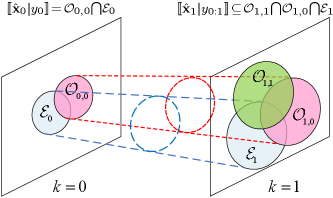
Before defining the OIT, let us first analyze how a single observed measurement affects the estimate as time elapses.999This is quite similar to analyzing the impulse response of a control system. At , from the update step (4) in Algorithm 1 we know that the estimate is the intersection of and , which describes how the observed measurement affects the estimate at . When we ignore all the successive observed measurements (like the impulse response does), only the prediction step in Algorithm 1 works for . Based on “set intersection under Minkowski sum”: for sets , and , we have101010The proof is as follows. , and such that . Since , we have for all . Thus, , , which implies , and we get (11).
| (11) |
and hence the estimate at is outer bounded by the intersection of the following two sets:
i.e., , which indicates how affects the estimate at . As such, we can analyze the effect of on the estimate at time . It defines the observation-information and state-evolution sets as follows.
Definition 5.
(Observation-Information and State-Evolution Sets) The observation-information set at time contributed by (i.e, the observed measurement at time ) is
| (12) |
The state-evolution set at time is
| (13) |
Remark 2.
Proposition 1.
(Set-Intersection-Based Outer B-ound) At , an outer bound on in Algorithm 1 is
| (14) |
which means and .
Proof.
See Appendix A. ∎
Note that
| (15) |
holds for any integer ,111111In this paper, when an integer is in an interval , this interval denotes . we define the Right-Hand Side (RHS) of (15) as the OIT (see Definition 6).
Definition 6 (Observation-Information Tower).
The OIT at time is the intersection of the observation-information sets over : .
Now, we provide a sufficient condition for the uniform boundedness (see Section 1) of the OIT as follows, which is fundamental to the results derived in the rest of this paper.
Theorem 1 (Uniform Boundedness of OIT).
Proof.
See Appendix B. ∎
Note that the uniform boundedness of the OIT indicates the diameter of () cannot go unbounded as , which is upper bounded by (16).
4 Stability Analysis of Classical Linear Set-Membership Filtering Framework
In this section, we study the stability issue w.r.t. the initial condition of the classical linear SMFing framework to address Problem 1, based on the OIT.
Since the uniform boundedness of the OIT requires observability, for general we introduce the observability decomposition: there exists a nonsingular such that the equivalence transformation transforms (1) and (2) into121212The observability decomposition follows Theorem 6.O6 in [5]: and , where , , , and , such that , , , , , and . Note that the eigenvalues of only depends on but independent of .
| (17) |
where and ; the pair is observable with the observability index ; it is well-known that is detectable if and only if , where returns the spectral radius of a matrix.
Now, we propose a stability condition of the classical linear SMFing framework as follows, where we define and as the projections of to the subspaces w.r.t. and , respectively.
Theorem 2 (Stability Criterion).
The classical SM-Fing framework in Algorithm 1 is stable w.r.t. its initial condition, if the following conditions hold:
-
(i)
;
-
(ii)
.
Proof.
See Appendix C. ∎
Remark 3.
Theorem 2 tells that when conditions (i) and (ii) hold, the classical SMFing framework is stable, which solves Problem 1. More precisely, these two conditions ensure the well-posedness and the bounded estimation gap, respectively. However, under condition (i), we cannot always keep (which is different from Proposition 4 in Appendix C for observable systems), i.e., the outer boundedness breaks.
As mentioned in Remark 3, condition (ii) in Theorem 2 is a sufficient condition for the boundedness of the estimation gap. To evaluate the difference between the sufficiency and the necessity, we provide a necessary condition for the bounded estimation gap in Proposition 2.
Proposition 2.
(Necessary Condition for Bounded Estimation Gap) For all bounded with , if the estimation gap of Algorithm 1 is bounded, must be marginally stable131313In this paper, it refers to that is the system matrix of a marginally stable discrete-time system, i.e., all eigenvalues of have magnitudes less or equal to one and those equal to one are non-defective [5]..
Proof.
See Appendix D. ∎
Remark 4.
For all bounded with , the proposed sufficient condition for the bounded estimation gap [i.e., condition (ii) in Theorem 2] is very close to the necessary condition given in Proposition 2. When , condition (ii) means is marginally stable; in that case, it becomes a necessary and sufficient condition. When , in general we need (which is close to marginal stability of ), i.e., is detectable, to provide the bounded-input bounded-output stability to guarantee the bounded estimation gap.
The following corollary gives a sufficient condition for simultaneously guaranteeing the stability w.r.t. the initial condition and the uniform boundedness of the estimate.
Corollary 1 (Egregium).
For bounded with , the classical SMFing framework is stable w.r.t. the initial condition and has the uniformly bounded estimate w.r.t. if is detectable.
Proof.
See Appendix E. ∎
Remark 5.
provides an explicit condition for the stability and the uniform boundedness141414Even though the detectability is usually assumed for the uniform boundedness [7], to be best of our knowledge, there are no existing results on rigorously proving it.. This result is consistent with the discrete-time Kalman filter that detectable implies a stable151515For Kalman filters, to achieve asymptotic stability w.r.t. the initial condition needs an additional condition on the reachability w.r.t. process noises. For linear SMFs, even though the numerical results in Section 7.1 show the asymptotic stability, proving it requires to introduce probability measures, which is beyond the scope of this work. filter [15]. Thus, it builds an important bridge between stochastic and non-stochastic linear filters on their stability w.r.t. initial conditions. It should also be highlighted that our result is independent of the types of the noises; while for stochastic filtering very few results are on the stability of discrete-time linear optimal filters with non-Gaussian noises.
Remark 6.
(Instability Caused by Improper Initial Conditions) Different from Kalman filtering, the classical linear SMFing framework is not stable for all bounded initial conditions. If the designer has little information on , it would be hard to choose a proper to guarantee the stability w.r.t. the initial condition (see Theorem 2). This motivates us to propose a stability-guaranteed filtering framework without using the knowledge of , presented in Section 5.
5 Stability-Guaranteed Filtering Framework
In this section, we establish a stability-guaranteed filtering framework, called OIT-inspired filtering (see Algorithm 2), to solve Problem 2.
From Theorem 2, we know that the initial condition should satisfy to ensure the stability of Algorithm 1 w.r.t. the initial condition. This motivates us to choose a sufficiently large so that the ill-posedness can be fully handled. However, it is difficult to choose such due to the following two issues:
-
•
Since is unlikely to know exactly, we can hardly guarantee .
-
•
Larger can increase the possibility of the inclusion but brings more conservativeness.
In the existing SMFing framework, these two issues cannot be effectively resolved. Thus, we propose a new SMFing framework inspired by OIT, with the help of the following lemma.
Lemma 1 (OIT-Inspired Invariance).
For all , where is the index of eigenvalue of (if does not contain eigenvalues, ), define the family of nested sets , in which is a closed -cube of edge length centered at . Then, s.t. , (18) holds, where is a submatrix formed by the first rows of .
| (18) |
Proof.
See Appendix F, which is inspired by OIT. ∎
Remark 7.
A line-by-line explanation of Algorithm 2 is as follows. Line 1 initializes the algorithm. Lines 2-7 give the filtering process at each . For , the estimate is identical to that of Algorithm 1 (see Line 3 of Algorithm 2), if it is not an empty set; otherwise, it will be reset by Line 5. In Line 5, we can choose with sufficiently large , which is used in Algorithm 3. For , the estimate is determined by Line 7. Note that Line 7 can be implemented in a recursive manner by its definition in (7).161616Generally speaking, reduction methods are required to balance the accuracy and the complexity in Line 7 for specific filter designs. But it is also possible to reduce the complexity without any accuracy loss (see the cases in Section 7.1).
Theorem 3 (Stability of OIT-Inspired Filtering).
Proof.
See Appendix G. ∎
6 Stable and Fast Constrained Zonotopic SMF
In this section, we develop a constrained zonotopic SMF under the new framework described in Algorithm 2, where the OIT plays the pivotal role. This SMF is not only with guaranteed stability but also with high efficiency and good accuracy. We call it the OIT-inspired Constrained Zonotopic SMF (OIT-CZ SMF).
Before presenting the SMF, we introduce the constrained zonotope [24] in Definition 7 with a small extension.
Definition 7 (Extended Constrained Zonotope).
A set is an (extended) constrained zonotope if there exists a quintuple such that is expressed by
where is the th component of .
In Definition 7, we slightly generalize the constrained zonotope in [24] by replacing , i.e., , with . The benefit is twofold: (i) we allow to be infinity such that the posterior sets induced by unbounded prior sets (which is required by the SMFing framework in Algorithm 2) can be fully described; (ii) the numerical stability of our proposed algorithm is improved.
Based on Definition 7, if , , and are constrained zonotopes, the resulting and in Algorithm 1 are also constrained zonotopes without any approximations. Specifically, by defining
| (19) |
the prediction step (3) gives the exact with
| (20) |
and the update step (4) returns the exact with
| (21) |
The proof of (20) and (21) is straightforward from [24], by rewriting (4) as .
Now, we are ready to design the OIT-CZ SMF (see Algorithm 3), where Proposition 3 plays an important role.
Proposition 3.
The image of a constrained zonotope under the filtering map is
| (22) |
where the parameters are given in (23) with and for .
| (23) |
Proof.
Algorithm 3 is under the framework of Algorithm 2, and we provide the line-by-line explanation as follows.
-
•
Line 1 initializes Algorithm 3, with the additional parameters and that: a larger leads to higher accuracy but increases the complexity (determined by Line 8); a smaller makes the estimate corresponding to the unobservable system more accurate but brings slower convergence of (24) [indicated by Line 12 and (88)]. Line 1 also gives an important constant in estimating the unobservable state (see Line 8 with Line 12).171717Note that can be calculated within finite steps (implied by the proof of Lemma 4). Thus, can be computed by searching over .
-
•
Lines 3-6 are for . Similarly to Lines 3 and 5 of Algorithm 2, Lines 3 and 5 of Algorithm 3 give the estimate : Line 3 gives the estimate returned by the constrained zonotopic version of Algorithm 1, i.e., with (19)-(21); in Line 5, can be expressed by for improving the numerical stability, where is the identity matrix of size and is the -dimensional all-ones column vector; one can double from until , and this can be done in finite steps. Line 6 calculates the interval hull of by simply solving linear programmings, where and are the generator matrix and the center of the resulting interval hull, respectively, and is employed to improve the numerical stability; note that is the projection of to the subspace w.r.t. , where is derived during the processing of calculating in Line 3 or Line 5.
-
•
Lines 8-12 are for , where and are the projections of to the subspaces w.r.t. and , respectively. Line 8 of Algorithm 3 gives the estimate , which is a finite-horizon version of Line 7 of Algorithm 2 over the time window . In Line 8, is derived based on Lemma 1,181818When utilizing Lemma 1, one should regard , , and as , , and , respectively. For , one can double from until the equality in (18) holds, where the equality can be checked by calculating interval hulls. and from Algorithm 3 we can observe that is calculated by Line 6 (for ) and Lines 9-12 (for ).191919In Line 8, we can replace with to improve the efficiency when is calculated (see Section 7.2). Line 9 gives the interval hull of the “input” of the unobservable subsystem, where is the center of the resulting interval hull and is diagonal and positive semi-definite. In Line 10, represents the maximum half-edge length of the interval hull derived by Line 9. Thus, records the greatest maximum half-edge length up to , which determines the radius (in the sense of -norm) of [see Line 12, where ]; for the center of , it is calculated by Line 11.
The following theorem describes not only the stability w.r.t. the initial condition but also two important properties of Algorithm 3. More specifically, for detectable : the finite-time inclusion property fixes the “outer boundedness breaking” problem in the classical linear SMFing framework (see Remark 3); the uniform boundedness of is guaranteed, i.e., the estimate cannot go unbounded as time elapses – to the best of our knowledge it is the first time to propose a constrained-zonotopic SMF with rigorously proven uniform boundedness.
Theorem 4 (Properties of OIT-CZ SMF).
Proof.
See Appendix H. ∎
Furthermore, Algorithm 3 has low computational complexity per step, especially when the system is observable: the averaged complexity for is determined by the case with (i.e., Lines 8-12 in Algorithm 3); for observable , only Line 8 remains, and we can also set ; from (23) we know that In Section 7.2.2, we show that Algorithm 3 has higher time efficiency compared with two most efficient constrained zonotopic SMFs in the toolbox CORA 2024 [1].
In terms of the accuracy, Algorithm 3 can be regarded as a reduction on the optimal estimate in Algorithm 1 with constrained zonotopic descriptions. Different from the existing reduction methods (e.g., [24]) based on geometric properties of constrained zonotopes, Algorithm 3 utilizes the properties of the dynamical system. Thus, the reduction is in a long-term manner instead of a greedy/instanetous manner, which greatly overcomes the wrapping effect. Therefore, the proposed OIT-CZ SMF has the desired performance improvement in terms of both complexity and accuracy.
7 Numerical Examples
7.1 Classical and Stability-Guaranteed Frameworks
In this subsection, we consider observable and detectable dynamical systems as illustrative examples to validate the theoretical results in Section 4 and Section 5.
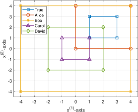
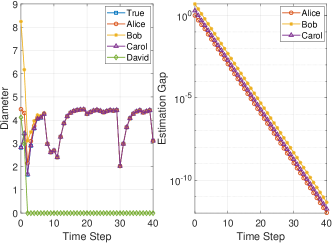
Observable : Consider a discretized second-order system described by (1) and (2), with parameters
| (25) |
which means is not Schur stable and is observable with . The true initial set is .202020The probability distributions of uncertain variables can be arbitrary for simulations. In Section 7, these uncertain variables are set to be uniformly distributed in their ranges. The Matlab codes for all results in this paper are provided at https://github.com/congyirui/Stability-of-Linear-SMF-2024.
Assume that there are four designers Alice, Bob, Carol, and David to design SMFs for (25), and the true initial set is unknown to them. Alice, Bob, and David employ the classical filtering framework in Algorithm 1, while Carol uses the OIT-inspired filtering framework in Algorithm 2, where .212121Note that the exact solutions of Algorithm 1 and Algorithm 2 can be derived by employing halfspace-representation-based method with acceptable computational complexities. From Fig. 2, we can see that the difference of the initial conditions chosen by the first three designers are corrected by the measurements , and the estimates converge to ; thus, the estimation gaps of these three filters are for ; this implies the estimation gaps are bounded for which corroborates the results in Theorem 2 and Theorem 3. In contrast, the initial condition chosen by David does not satisfy condition (i) in Theorem 2, and the resulting estimate becomes empty as time elapses.
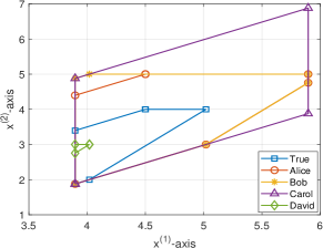
Detectable : Consider the system with
| (26) |
which implies is not Schur stable and is detectable with . The true initial set is .
The initial conditions chosen by Alice, Bob, Carol, and David are identical to those in Fig. 2, where Algorithm 2 is with . Fig. 3 corroborates the theoretical results in Theorem 2 and Theorem 3, where the estimation gaps corresponding to non-empty estimates are bounded; more specifically, they converge to exponentially fast.
7.2 The Stable and Fast Constrained Zonotopic SMF
Firstly, we use Monte Carlo simulation to test the OIT-CZ SMF in Section 7.2.1; then, we show the time efficiency of the OIT-CZ SMF in Section 7.2.2.
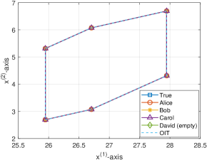
7.2.1 Interval hull of the estimate
In this part, we employ the OIT-CZ SMF to derive the interval hull of the estimate.
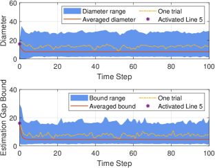
First, consider the randomly generated (by using drss function in MATLAB) with observable .
The process and measurement noises are with and .
The true initial set is , and the initial condition is , where is randomly generated in for testing Algorithm 3.
In the simulations, we set , , and (in Algorithm 3);
for each , the simulations are conducted times.
The results are shown in Fig. 4, where one of the simulation runs is highlighted by the (yellow) dash-dotted lines with the (purple) stars representing: holds in Line 4 of Algorithm 3 and Line 5 derives a non-empty by resetting .
We can see that the proposed OIT-CZ SMF is stable and uniformly bounded, which corroborates the theoretical results in Theorem 4.
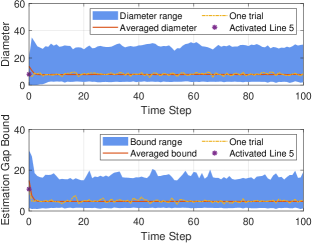
Second, consider the randomly generated (by using drss function in MATLAB) with detectable .
For the unobservable subsystem, is a randomly created matrix with ; each element in and is randomly selected from .
The transformation matrix is a randomly derived orthogonal matrix such that by (17): , , are finally obtained.
The sets , , , and the same as those in the simulations for observable .
Also, we set , , , and .
for each , the simulations are conducted times.
The results are shown in Fig. 4, which validates the results in Theorem 4.
7.2.2 Time Efficiency
In this part, we set222222If , the classical algorithm can return an error due to the ill-posedness. and compare the computation time (w.r.t. the constrained zonotopic description) of the proposed OIT-CZ SMF and two classical constrained zonotopic SMFs; these two classical SMFs are with the reduction methods girard and combastel in CORA 2024 [1], respectively. Consider the randomly generated observable systems same as those in Section 7.2.1, but with . We also set in Algorithm 3. For these two classical SMFs, we set and the degrees-of-freedom order [24] . The simulations are conducted for runs over the time window by using Matlab 2019b on a laptop with Intel Core [email protected] CPU, and the averaged computation time (per time step) is shown in Table 1. Note that the diameters in the sense of -norm for SMF (girard), SMF (combastel), and OIT-CZ SMF are respectively: , , and (when ); , , and (when ); , , and (when ). These results show that the OIT-CZ SMF achieves significantly higher accuracy with several orders of magnitude reduction in computation time, as compared to the classical SMFs.
| SMF (girard) | s | s | s |
|---|---|---|---|
| SMF (combastel) | s | s | s |
| OIT-CZ SMF | s | s | s |
8 Conclusion
In this paper, the stability of the SMFs w.r.t. the initial condition has been studied for linear time-invariant systems. Specifically, the stability is given by the well-posedness and the bounded estimation gap. Based on our proposed OIT, we have analyzed the stability of the classical linear SMFing framework, where an explicit sufficient condition has been given. Then, we have provided a good necessary condition for the bounded estimation gap, which is very close to the sufficient condition. To avoid unstable filter design resulted from improper initial conditions, the OIT-inspired filtering framework has been established to guaranteed the stability. Under this new framework, we have developed the OIT-CZ SMF with guaranteed stability, uniform boundedness, high efficiency, and good accuracy.
References
- [1] Althoff, M., Kochdumper, N., & Wetzlinger, M. CORA 2024 manual. 2024.
- [2] Althoff, M. & Rath, J.J. Comparison of guaranteed state estimators for linear time-invariant systems. Automatica, 130:109662, Aug. 2021.
- [3] Becis-Aubry, Y. Ellipsoidal constrained state estimation in presence of bounded disturbances. arXiv:2012.03267, 2021.
- [4] Becis-Aubry, Y., Boutayeb, M., & Darouach, M.. State estimation in the presence of bounded disturbances. Automatica, 44(7):1867–1873, Jul. 2008.
- [5] Chen, C.T. Linear System Theory and Design. New York, NY, USA: Oxford University Press, 3rd edition, 1999.
- [6] Chen, J. & Gu, G. Control-oriented system identification: an approach. New York, NY, USA: John Wiley & Sons, 2000.
- [7] Combastel, C. A state bounding observer based on zonotopes. In Proc. Eur. Control Conf. (ECC), pages 2589–2594, Sep. 2003.
- [8] Combastel, C. Zonotopes and kalman observers: Gain optimality under distinct uncertainty paradigms and robust convergence. Automatica, 55:265–273, May 2015.
- [9] Cong, Y., Zhou, X., & Kennedy, R.A. Finite blocklength entropy-achieving coding for linear system stabilization. IEEE Trans. Autom. Control, 66:153–167, Jan. 2021.
- [10] Cong, Y., Wang, X., & Zhou, X. Rethinking the mathematical framework and optimality of set-membership filtering. IEEE Trans. Autom. Control, 67(5):2544–2551, May 2022.
- [11] Fei, Z., Yang, L., Sun, X., & Ren, S. Zonotopic set-membership state estimation for switched systems with restricted switching. IEEE Trans. Autom. Control, 67(11):6127-6134, Nov. 2021.
- [12] Jazwinski, A.H. Stochastic Processes and Filtering Theory. New York, USA: Academic Press, New York, NY, USA, 1970.
- [13] Kalman, R.E. & Bucy, R.S. New results in linear filtering and prediction theory. J. Basic Eng., 83(1):95–108, 1961.
- [14] Kühn, W. Rigorously computed orbits of dynamical systems without the wrapping effect. Computing, 61(1):47–67, Mar. 1998.
- [15] Lewis, F., Xie, L., & Popa, D. Optimal and robust estimation: with an introduction to stochastic control theory. CRC Press, Boca Raton, FL, USA, 2ed. edition, 2007.
- [16] Liu, Y., Zhao, Y., & Wu, F. Ellipsoidal state-bounding-based set-membership estimation for linear system with unknown-but-bounded disturbances. IET Control Theory & Appl., 10(4):431–442, Feb. 2016.
- [17] Loukkas, N., Martinez, J.J., & Meslem, N. Set-membership observer design based on ellipsoidal invariant sets. IFAC-PapersOnLine, 50(1):6471–6476, Jul. 2017.
- [18] Mazenc, F. & Bernard, O. Interval observers for linear time-invariant systems with disturbances. Automatica, 47(1):140–147, Jan. 2011.
- [19] Milanese, M., Norton, J., Piet-Lahanier, H., & Walter, É. Bounding Approaches to System Identification. New York, NY, USA: Plenum Press, 1996.
- [20] Milanese, M., Tempo, R., & Vicino, A. Robustness in Identification and Control. New York, NY, USA: Plenum Press, 1989.
- [21] Nair, G.N. A nonstochastic information theory for communication and state estimation. IEEE Trans. Autom. Control, 58(6):1497–1510, Jun. 2013.
- [22] Ocone, D. & Pardoux, E. Asymptotic stability of the optimal filter with respect to its initial condition. SIAM J. Control Optim., 34(1):226–243, 1996.
- [23] Särkkä, S. Bayesian filtering and smoothing. Cambridge University Press, New York, NY, USA, 2013.
- [24] Scott, J.K., Raimondo, D.M., Marseglia, G.R., & Braatz, R.D. Constrained zonotopes: A new tool for set-based estimation and fault detection. Automatica, 69:126–136, Jul. 2016.
- [25] Shen, Q., Liu, J., Zhou, X., Zhao, Q., & Wang, Q. Low-complexity ISS state estimation approach with bounded disturbances. Int. J. Adaptive Control and Signal Process., 32(10):1473–1488, Aug. 2018.
- [26] Handel, R. Filtering, stability, and robustness. PhD thesis, California Institute of Technology, 2006.
- [27] Wang, Y., Puig, V., & Cembrano, G. Set-membership approach and kalman observer based on zonotopes for discrete-time descriptor systems. Automatica, 93:435–443, Jul. 2018.
- [28] Wang, Y., Wang, Z., Puig, V., & Cembrano, G. Zonotopic set-membership state estimation for discrete-time descriptor LPV systems. IEEE Trans. Autom. Control, 64(5):2092–2099, Aug. 2019.
- [29] Xu, F., Tan, J., Raïssi, T., & Liang, B. Design of optimal interval observers using set-theoretic methods for robust state estimation. Int. J. Robust and Nonlinear Control, 30(9):3692–3705, Jun. 2020.
Appendix A Proof of Proposition 1
We prove Proposition 1 by induction.
Inductive step: Assume (14) holds for any . For , the prior set is derived by (3) that
| (27) |
where is established by (11), and is from the following two equations:
| (28) | ||||
| (29) |
where and follow from for any linear map . By (27) and (4), the posterior set is outer bounded by
which implies (14) holds for . Thus, Proposition 1 is proven by induction.
Appendix B Proof of Theorem 1
To start with, we provide two lemmas as follows.
Lemma 2.
(Uniform Boundedness Invariance Under Linear Map) , let the set be uniformly bounded w.r.t. , and the linear map be independent of . Then, is uniformly bounded w.r.t. .
Proof.
Since , is uniformly bounded w.r.t. , there exists a such that . Thus, , the following holds for all
| (30) |
where is the operator norm of . Now, we have ,
| (31) |
where inequality can be easily obtained by using the following triangle inequality: for the sets (),
| (32) |
By (31), is uniformly bounded. ∎
Lemma 3 (Uniformly Bounded Intersection).
(), let be any uniformly bounded set w.r.t. . Then,
| (33) |
is uniformly bounded w.r.t. [recall that returns the range space of matrix ], if
| (34) |
where , and () satisfies .
Proof.
This proof has three steps. In the first step, we prove the following equality holds:
| (35) |
where and and stands for the Cartesian product. In the second step, we analyze from the perspective of solving linear equations. Afterwards, we complete this proof in the third step.
Step 1: Since , we are readily to use distributive law of sets to get (35). Specifically, we have232323The readers can use mathematical induction to derive a rigorous proof. Due to the page limit, we omit it here.
| (36) |
which means (35) holds.
Step 2: , with we have
which is the solution space of the linear equation . Thus, we get
| (37) |
where . With (34), we know that has either a unique solution or no solution, i.e., at most contains one element. Hence, we have
| (38) |
where .
Now, we prove Theorem 1. With (5), the observation-information set in (12) can be rewritten as
| (40) |
Thus, with (40), , and , we can rewrite the OIT in Definition 6 as
| (41) |
where
| (42) |
Let such that . By , (41) can be rewritten as
| (43) |
Since and , we know that and () are uniformly bounded w.r.t. . Hence, , by Lemma 2 is uniformly bounded w.r.t. . Now, the precondition of Lemma 3 is satisfied for (43). To guarantee the uniform boundedness of (43), we only need to prove condition (34) with in Lemma 3 holds, where . The proof has two steps.
Step 1: Prove . To be more specific, for non-singular , we show that
| (44) |
as follows: Firstly, we have
| (45) |
which implies . Secondly, we check the rank of as follows
| (46) |
Appendix C Proof of Theorem 2
Firstly, we consider the stability for observable , and a sufficient condition is provided in Proposition 4.
Proposition 4 (Stability of Observable Systems).
For observable and bounded , the classical SMFing framework in Algorithm 1 is stable and is uniformly bounded w.r.t. .
Proof.
We prove the well-posedness, the uniform boundedness of the estimate, and the boundedness of the estimation gap as follows.
Well-posedness: Since , with (4), we have
| (49) |
i.e., , where follows from the fact that is generated by (2) with at least one possible . With (3), we have , as . Similarly to (49), by (4), holds. Proceeding forward, we get for .
Uniformly bounded estimate: Let with a non-singular such that
| (50) |
where is non-singular and is a block diagonal matrix corresponding to all Jordan blocks associated with the eigenvalue . Thus, we have
| (51) |
where follows from the uniform boundedness252525Noticing that is a nilpotent matrix, we can derive the uniform boundedness of from and the boundedness of . of w.r.t. that: there exists a such that . Then, we only need to focus on the first subsystem of (50), i.e.,
| (52) |
where is an equivalent measurement noise [which is related to due to (50)] and is uniformly bounded w.r.t. . Define with
Note that is an observation-information set in terms of (52). Hence, we can derive .262626Even though and are related, we can assume the unrelatedness holds and employ Theorem 3 in [10] to employ (14) and (15) to get this result. Thus, for , where is the observability index w.r.t. , we get
| (53) |
where is defined in (16) with for the uniformly bounded equivalent noise . For , bounded lead to bounded (determined by Algorithm 1). Thus is uniformly bounded w.r.t. .
Bounded estimation gap: Due to the page limit272727We recommend the readers to follow the ideas in (58)-(68) and derive a tighter bound. However, the upper bound given in (54) is good enough to derive the boundedness of the estimation gap for observable systems., we provide the proof based on
| (54) |
where is from (see the proof of well-posedness). Therefore, for observable , the boundedness of the estimation gap is established. ∎
Now, we prove the stability of Algorithm 1 w.r.t. the initial condition under conditions (i) and (ii) of Theorem 2.
Well-posedness: Define with
Note that is an observation-information set in terms of the observable subsystem of (17). Then, we have
| (55) |
where follows from the non-singularity of ; is established by . Substituting into (55) and noticing that , we have
| (56) |
This means such that
where . Since in condition (i) holds, we get . Thus, such that , which together with (55) gives
| (57) |
From the first equalities of (56) and (57), we can derive , which combined with the observable subsystem in (17) yields . Proceeding forward, we can obtain that and for .
Boundedness of estimation gap: From Definition 3, the estimation gap can be upper bounded by
| (58) |
Noticing the structure of in (10), firstly we prove the upper boundedness of
| (59) |
Applying Proposition 4 to the observable subsystem of (17), we get that and , there exists a such that for . Thus, (59) can be upper bounded by
| (60) |
From the unobservable subsystem of (17), we have
| (61) |
where follows from and . Hence, , such that
| (62) |
Likewise, , such that
| (63) |
Therefore, (60) is upper bounded by
| (64) |
where [based on (62) and (63)]
| (65) |
By condition (ii), (65), and the uniform boundedness of and , there exists a such that
| (66) |
which yields the boundedness of (59).
Appendix D Proof of Proposition 2
The estimation gap can be lower bounded by
| (69) |
From (69) and (65), we know: if is not marginally stable, then there exists a bounded such that in (69) unboundedly increases with . Thus, for all bounded , the boundedness of the estimation gap cannot be guaranteed when is not marginally stable. Therefore, must be marginally stable to ensure the bounded .
Appendix E Proof of
By Theorem 2, the classical SMFing framework with bounded and is stable w.r.t. the initial condition if is detectable. Thus, we only focus on the uniform boundedness of the estimate.
From Proposition 4, is bounded. Thus, with
we know that is uniformly bounded w.r.t. if and only if is uniformly bounded w.r.t. . From (61) with [as is detectable], bounded , and uniformly bounded and , we can derive the uniform boundedness of . Therefore, is uniformly bounded w.r.t. for detectable .
Appendix F Proof of Lemma 1
Since for any , in (18) corresponds to the observable subsystem and the resulting set is independent of , without loss of generality, we consider the pair is observable, i.e., . In that case, (18) becomes
| (70) |
Firstly, we prove (70) for non-singular . Because for all , from Definition 1 we have
| (71) |
By Theorem 1, , is bounded, and s.t. :
| (72) |
which together with (14) and (15) gives for . Thus, , and with (71) we get (70).
Appendix G Proof of Theorem 3
Well-posedness: For , Line 5 resets every empty to a non-empty set. For , the estimate in Line 7 is non-empty, which is guaranteed by (see Remark 7) and the well-posedness part [see (55)-(57)] in the proof of Theorem 2. Thus, holds for .
Boundedness of estimation gap: For , bounded with Lines 3 and 5 indicates . For , using the same techniques in (58)-(68) [note that ensures the preconditon in Proposition 4 when it is applied to the observable system to derive (60)], we can obtain the boundedness of . Therefore, the estimation gap is bounded for .
Appendix H Proof of Theorem 4
Firstly, we provide Lemma 4 for bounding the norm of matrix power, which is a variant of Lemma 3 in [9].
Lemma 4 (Bound on Norm of Matrix Power).
Given with , for , holds for all , where .
Proof.
, let , and we have . Since , we can find a such that for all , the following holds
| (73) |
which implies . It together with 282828Note that and for . gives for all . ∎
When is detectable, the uniform boundedness of the estimate and the boundedness of the estimation gap can be readily derived based on the results in Section 5, when we replace and with and , respectively. Thus, we only focus on the well-posedness and finite-time inclusion property of Algorithm 3.
Well-posedness: Similarly to the well-posedness part in Appendix G (Lines 5 and 8 in Algorithm 3 play the same role as Lines 5 and 7 in Algorithm 2), we have for and
| (74) |
The only part needs highlighting is: for Line 8, when , Lemma 1 guarantees ; when , ; thus,
| (75) |
Boundedness of estimation gap: When is detectable, condition (ii) in Theorem 2 holds. Then, the proof is similar to that of Theorem 3.
Finite-time inclusion: The proof includes two steps. In the first step, we show that
| (76) |
holds for , where
| (77) |
In the second step, the finite-time inclusion property (24) is proven based on (76).
Step 1: We use the mathematical induction on (76).
Base case: For , we have . Thus, (76) holds for .
Inductive step: Assume (76) holds for any . For , with (17) we have
| (78) |
Noticing that and
| (79) |
we have [as ]
| (80) |
It implies , i.e., (76) holds for . Thus, (76) is proven by induction.
Step 2: We split the RHS of (77) as :
| (81) | ||||
| (82) |
Then, we also spilt in Line 12 into two parts:
| (83) |
where , , , and such that and . Next, we prove
| (84) |
for sufficiently large , and
| (85) |
such that
| (86) |
For (84), , its distance from the center of is upper bounded by
| (87) |
Since (81) implies , we can further derive that for given in Line 1, such that
| (88) |
which means , i.e., (84) holds.
For (85), as (74) holds, in (82) is bounded by
| (89) |
where follows from Lines 9-10 and the fact that gives the maximum edge length of the interval hull. Recall that and , and observe that