Stability of a passive viscous droplet in a confined active nematic liquid crystal
Abstract
The translation and shape deformations of a passive viscous Newtonian droplet immersed in an active nematic liquid crystal under circular confinement are analyzed using a linear stability analysis. We focus on the case of a sharply aligned active nematic in the limit of strong elastic relaxation in two dimensions. Using an active liquid crystal model, we employ the Lorentz reciprocal theorem for Stokes flow to study the growth of interfacial perturbations as a result of both active and elastic stresses. Instabilities are uncovered in both extensile and contractile systems, for which growth rates are calculated and presented in terms of the dimensionless ratios of active, elastic, and capillary stresses, as well as the viscosity ratio between the two fluids. We also extend our theory to analyze the inverse scenario, namely, the stability of an active nematic droplet surrounded by a passive viscous layer. Our results highlight the subtle interplay of capillary, active, elastic, and viscous stresses in governing droplet stability. The instabilities uncovered here may be relevant to a plethora of biological active systems, from the dynamics of passive droplets in bacterial suspensions to the organization of subcellular compartments inside the cell and cell nucleus.
I Introduction
The interaction of active materials with passive phases is relevant to many biological systems spanning a range of length scales. Examples on large scales include: front propagation in spreading bacterial swarms and suspensions, where complex interfacial instabilities have been observed Patteson et al. (2018); Martínez-Calvo et al. (2022); cell migration during the formation of cancer metastasis Nürnberg et al. (2011); Hoshino et al. (2013); or the migration of confluent epithelial cell layers during wound healing Martin and Parkhurst (2004); Armengol-Collado et al. (2023). On cellular length scales, the organization of various subcellular compartments and organelles hinges on their interaction with the active cytoskeleton and cytoplasmic flows Chu et al. (2017); Mogilner and Manhart (2018). On yet smaller scales, the placement and structural organization of subnuclear bodies and heterochromatin compartments inside the cell nucleus have been hypothesized to be affected by the dynamics of transcriptionally active euchromatin Caragine et al. (2018); Mahajan et al. (2022). Interfaces between active and passive phases have also been of interest in synthetic and reconstituted systems, e.g., in active nematic fluids composed of microtubules and molecular motors Sanchez et al. (2012); Shelley (2016), where activity has been shown to destabilize interfaces and drive shape fluctuations and active waves Adkins et al. (2022).
In all of these systems, the dynamics and emerging morphologies of active/passive interfaces stem from the interplay of active, elastic, viscous, and possibly capillary stresses. A perturbation to the interfacial shape affects the orientation of the active matter constituents, thus giving rise to both active and elastic stresses. These stresses in turn result in tractions on the interface as well as flows in the material, whose net effect can be either stabilizing or destabilizing. A few theoretical and computational models have been proposed in recent years to explain these effects. The dynamics of active droplets, either in free space or near boundaries, has been studied numerically and analytically, where active stresses and the flows they induce can lead to spontaneous propulsion, fingering instabilities, division or spreading Tjhung et al. (2012); Joanny and Ramaswamy (2012); Giomi and DeSimone (2014); Whitfield et al. (2014); Khoromskaia and Alexander (2015); Young et al. (2021); Alert (2022). Active films have also been considered, where interfacial instabilities can either be triggered or stabilized by activity depending on the sign of active stresses Voituriez et al. (2006); Sankararaman and Ramaswamy (2009); Blow et al. (2017); Alonso-Matilla and Saintillan (2019). Other studies have analyzed the motion of passive objects, either rigid or deformable, suspended in active suspensions, where active stresses can give rise to spontaneous transport Freund (2023, 2024), rotation Fürthauer et al. (2012), and deformations Chandler and Spagnolie (2024).
In the present work, we analyze a canonical system consisting of a passive viscous Newtonian droplet immersed in an active nematic liquid crystal under circular confinement. The opposite scenario of an active nematic droplet surrounded by a passive viscous layer is also addressed. We consider the sharply aligned limit for the nematic, and use strong anchoring boundary conditions at the interface and domain boundaries, a regime where the configuration of the nematic field is entirely governed by the system’s geometry. Using a linear stability analysis along with the Lorentz reciprocal theorem Masoud and Stone (2019), we study the stability of the drop under both translation and deformation, and calculate growth rates in terms of the governing parameters. We uncover instabilities in both extensile and contractile systems, which may be relevant to a wide range of biological active systems, from the dynamics of passive droplets in bacterial suspensions to the organization of subcellular compartments inside the cell and cell nucleus.
The paper is organized as follows. We formulate the problem in Sec. II, where we present the governing equations, boundary conditions, and non-dimensionalization. Section III presents details of the linear stability analysis of the axisymmetric base state and a discussion of the dispersion relation and growth rates. The inverted problem, i.e., the stability of an active nematic drop within a passive layer and its associated dispersion relation are discussed in Sec. IV. We conclude in Sec. V.
II Problem formulation
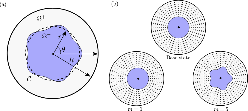
We analyze the stability of a viscous Newtonian droplet surrounded by a sharply aligned active nematic fluid in circular confinement in two dimensions (Fig. 1). The system is enclosed by a circular boundary of radius centered at the origin . In polar coordinates , the shape of the interface between the drop and nematic layer is described by the Monge representation , where is the dimensionless radius ratio, and captures deviations from the reference base state where the drop is circular and centered at the origin. We denote by the domain occupied by the passive drop, by the domain occupied by the nematic, and by the curve describing the shape of the interface between them.
II.1 Nematodynamics
Orientational order in the active nematic layer surrounding the droplet is described by a nematic director field (with in the sharply aligned limit), which satisfies the Leslie-Ericksen model Ericksen (1961, 1962); Leslie (1968); De Gennes and Prost (1995); Gao et al. (2017)
| (1) |
where is the fluid velocity in the nematic. The rate-of-strain tensor and rate-of-rotation tensor depend on the velocity gradient defined as , and denotes the flow alignment parameter. The last term in Eq. (1) captures nematic elasticity, and involves the rotational viscosity and molecular field , which derives from a free energy density. Under the commonly used one-constant approximation De Gennes and Prost (1995), we express the free energy density as
| (2) |
from which the molecular field is obtained as
| (3) |
Nematic elasticity thus enters Eq. (1) as a diffusive term, with the ratio playing the role of a diffusivity. The nematic is assumed to satisfy strong parallel anchoring conditions at both the outer domain boundary and droplet interface. Note that in two dimensions the director field is equivalently described by a single angle such that ; we make further use of this representation below.
II.2 Mass and momentum balance
Conservation of mass and momentum in the active nematic read
| (4) |
where , and are the hydrodynamic, active, and elastic (or Leslie-Ericksen) stress tensors, respectively:
| (5) | ||||
| (6) | ||||
| (7) |
Here, is the fluid pressure and is the shear viscosity of the fluid. The active stress magnitude is , where is the number density of active dipoles and is the dipole strength or stresslet; for an extensile nematic, and in the contractile case Saintillan and Shelley (2013); Saintillan (2018).
In the passive viscous drop, the only stress is hydrodynamic, and the governing equations are
| (8) |
where and . Here and in the following, variables associated with flow inside the drop are decorated with an overbar.
II.3 Boundary conditions
At the outer boundary , the no-slip condition applies. There, the nematic director is tangent to the boundary: .
To parametrize the shape of the drop, we introduce the function and note that the interface between the two fluids is defined as . Consequently, the outward unit normal to the interface is
| (9) |
The kinematic boundary condition describing the evolution of the interface is
| (10) |
i.e.,
| (11) |
Note that the fluid velocity is continuous at the interface: at .
Neglecting Marangoni effects, the dynamic boundary condition is given by the stress balance
| (12) |
where is the surface tension, assumed to be uniform, and is the local curvature. The parallel anchoring condition for the nematic at the drop surface reads: at .
II.4 Non-dimensionalization
We scale the equations using length scale , time scale , and velocity scale . The nematodynamic equation (1) becomes
| (13) |
where the active Péclet number compares the effects of the fluid flow to nematic relaxation on the dynamics of .
In the rest of the paper, we will assume (strong nematic relaxation), in which case the equation for simplifies to
| (14) |
In this limit, the configuration of the nematic is thus purely a boundary value problem governed by the geometry of the nematic layer through the anchoring boundary conditions. The only effect of the flow on is through the kinematic boundary condition (11), which governs the shape of the interface.
In the nematic, we use to scale the pressure and stress. The stress tensors inside the active nematic then become
| (15) |
Note that the elastic stress was simplified under that assumption of and by making use of Eq. (14), and that its isotropic part is henceforth omitted as it can absorbed in the fluid pressure. Inside the passive drop, the hydrodynamic stress reads
| (16) |
where is the viscosity ratio. The active stress coefficient in Eq. (15) is , with for an extensile nematic and for a contractile nematic. The relative magnitude of elastic over active stresses is captured by the dimensionless parameter , or ratio of the active length scale to the system size. Active stresses are negligible when , whereas they dominate when , a regime where active turbulence is typically observed. In the present work, we assume .
The kinematic boundary condition (11) remains unchanged under non-dimensionalization, and the stress balance (12) becomes
| (17) |
where we have introduced the active capillary number comparing the magnitudes of active vs. capillary stresses. Under the assumption of vanishing Péclet number, the system is entirely governed by five parameters: the radius ratio , the sign of active stresses, the capillary number , the dimensionless elastic constant , and the viscosity ratio .
III Linear stability analysis
We analyze the stability of small perturbations from the stable case of a circular drop () centered at the origin. In the following, subscripts 0 and 1 are used to denote the base state and linear perturbations, respectively.
III.1 Circular base state
In the unperturbed state where the drop is circular and centered at the origin (), the nematic field lines are concentric circles with
| (18) |
which satisfies Eq. (14) along with the anchoring boundary conditions at and . The corresponding nematic director is . Both fluids are still (). The base-state active and elastic stress tensors in the outer nematic layer are given by
| (19) |
They both induce a pressure gradient in the nematic fluid:
| (20) |
from which
| (21) |
The pressure inside the passive drop is uniform and is dictated by the stress balance (17):
| (22) |
III.2 Domain perturbation and linearized nematic field
Leveraging periodicity in the direction, we perturb the shape of the interface with an azimuthal Fourier mode
| (23) |
where and . We assume to be given, and our goal is to analyze the growth of the perturbation amplitude . At linear order, the perturbed outward normal and curvature along the interface are, respectively,
| (24) | ||||
| (25) |
The instantaneous shape of the interface fully governs that of the nematic field lines. The director angle is expanded as . The boundary conditions on the perturbation angle are at , and
| (26) |
A solution of Laplace’s equation that satisfies both of these conditions is readily obtained by separation of variables,
| (27) |
and the corresponding expansion for the nematic director follows as
| (28) |
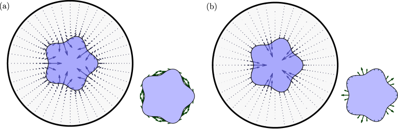
Typical director fields corresponding to and are illustrated in Fig. 1(b,c).
III.3 Linearized active and elastic stresses
III.4 Linearized flow problem and boundary conditions
The fluid velocity and pressure perturbations satisfy the Stokes equations (4) and (8) at linear order in :
| (32) | ||||
| (33) |
where the active and elastic stresses in Eq. (32) are known from Eqs. (29) and (31). The flows in the two regions are coupled via the dynamic boundary condition (17), which applies at .
Our method of solution, described in Sec. III.5, will rely on the Lorentz reciprocal theorem for Stokes flow Masoud and Stone (2019). To this end, it is convenient to first recast the flow problem around a circular boundary (). Note that Eqs. (32)–(33) remain unchanged around the circle to linear order. We also need to apply the dynamic boundary condition (17) on the circle, which is achieved by expanding the various fields involved in the boundary conditions as Taylor series in the neighborhood of . For example, the stress tensor can be expanded as:
| (34) |
Inserting Eq. (34) into Eq. (17), linearizing, and simplifying using Eqs. (19)–(22), we obtain the following dynamic boundary condition at ,
| (35) |
Finally, the linearized kinematic boundary condition (11) reads
| (36) |
In this linearized problem, Eq. (36) is an amplitude evolution equation on the inner circle, driven by the solution of the two boundary value problems inside the inner circle and the outer annulus. This reduction allows the use of the Lorentz reciprocal theorem in the circular geometry as we describe next.
III.5 Lorentz reciprocal theorem
We apply the Lorentz reciprocal theorem Masoud and Stone (2019) to the linear problem of Eqs. (32)–(36) in the annular geometry with a circular boundary. To this end, we introduce an auxiliary flow problem in the same annular geometry, in which both fluids are passive and the flow is driven by a prescribed stress jump at the interface. In this problem, both fluids are Newtonian with viscosity ratio and the interface between them is circular and centered at the origin (). We use uppercase fonts (, , ,…) for all variables associated with the auxiliary problem. The flow in both fluid regions is governed by the homogeneous Stokes equations,
| (37) | ||||
| (38) |
Here, and are the Newtonian stress tensors, where and are the respective rate-of-strain tensors. The velocity satisfies the no-slip condition at the outer boundary: , and is continuous at the interface: . The flow is driven by a prescribed jump in normal tractions at the interface:
| (39) |
where is an arbitrary constant. In two dimensions, this Newtonian problem is readily solved in terms of two streamfunctions and such that
| (40) |
with similar expressions for the streamfunction and its derivatives inside the drop. The two dimensionless functions and can be obtained analytically by the solution of the Stokes equations; details of their solutions are presented in the Appendix.
Using Eqs. (32) and (37) in the outer nematic fluid region and relying on the symmetry of the stress tensors, it is straightforward to derive the two relations
| (41) | ||||
| (42) |
Subtracting Eq. (42) from Eq. (41), integrating over the outer region , and applying the divergence theorem then yields
| (43) |
where denotes the circular interface at . Note that the boundary term at vanished due to the no-slip condition, and that we used that to simplify the right-hand side. Following an identical process in the inner region , we obtain,
| (44) |
which does not involve any bulk integral since active and elastic stresses are absent inside . Combining Eqs. (43) and (44), we obtain
| (45) |
which is the central statement of the reciprocal theorem. The first contribution to the contour integral on the left-hand side can be simplified using the linearized kinematic boundary condition (36) along with the auxiliary stress balance (39), yielding
| (46) |
Similarly, the second term in the contour integral can be simplified using the linearized dynamic boundary condition (35) along with Eq. (40) for the auxiliary velocity:
| (47) | ||||
| (48) |
Finally, the surface integral on the right-hand side of Eq. (45) can be evaluated using Eqs. (29) and (31) for the linearized active and elastic stresses:
| (49) | ||||
| (50) | ||||
III.6 Dispersion relation and growth rates
Upon inserting Eqs. (46), (48) and (50) into the reciprocal relation (45), the arbitrary stress jump magnitude can be eliminated, and we arrive at a first-order ODE for the interfacial perturbation amplitude,
| (51) |
The constant growth rate for normal mode includes contributions from capillary, active and elastic stresses:
| (52) |
respectively given by
| (53) | ||||
| (54) | ||||
| (55) |
These various growth rates depend on the function appearing in the solution of the Newtonian auxiliary problem, whose form differs between the translation () and deformation () modes of the drop. We analyze and discuss these two cases separately.
III.6.1 Translation mode
The first normal mode captures translation of the drop and is the only mode with a non-zero displacement of the drop center of mass. At linear order, it does not affect the curvature of the drop, and therefore the growth is unaffected by surface tension: . The function for is given in Eq. (A-6). Inserting this expression into Eqs. (54) and (55) and simplifying provides the active and elastic growth rates,
| (56) | ||||
| (57) |
where the coefficients , , and are dimensionless functions of and given by Eqs. (A-7)–(A-9) of the Appendix.
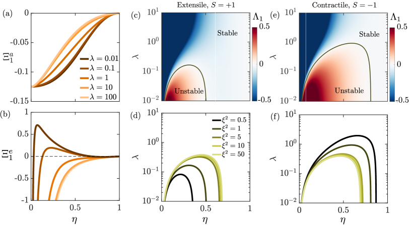
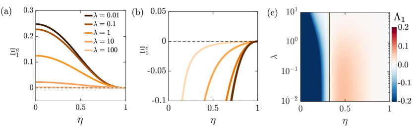
The two functions and are plotted vs for different viscosity ratios in Fig. 2(a,b). As seen in Fig. 2(a), for all values of and , indicating that the translational mode is linearly stable under active stresses in extensile systems, but unstable in contractile systems (recall that gets multiplied by in Eq. (52) for the actual growth rate). only shows a weak dependence on viscosity ratio. The two asymptotes for a rigid particle () and an inviscid bubble () are given by
| (58) |
The elastic contribution shows a more complex dependence on both and in Fig. 2(b). High-viscosity drops are always stable under elastic stresses. As decreases, an unstable region appears at intermediate values of . Regardless of , we find that as , i.e., very small drops are always stable to translation. The divergence of the growth rate in that limit is attributed to the divergence of the base-state elastic pressure at the origin when as seen in Eq. (21). When both active and elastic stresses play a role, the translational mode can be either stable or unstable depending on parameter values. For the extensile case, this is illustrated in Fig. 2(c), showing a color plot of the total growth rate in the parameter space: the system is primarily stable, except in the red region which occurs at intermediate values of and low viscosity ratios. The dependence of the marginal stability curve on is shown in Fig. 2(d), where increasing the magnitude of elastic stresses is found to increase the size of the unstable region. The contractile case is analyzed similarly in Fig. 2(e,f): the unstable region is found to be larger in that case, but to decrease in size with increasing .
Some partial intuition into the trends observed in Fig. 2 can be obtained by analyzing the active and elastic stresses exerted in the bulk of the nematic and on the interface. The active and elastic force densities exerted in the bulk are given by the divergence of the respective stress tensors, and . At linear order and for , their components are given by
| (59) |
and
| (60) |
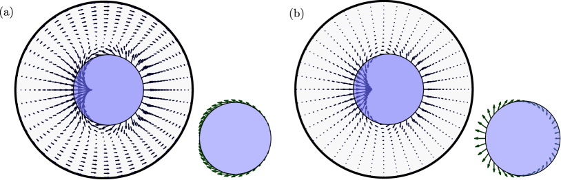
The two force fields are shown in Fig. 3 for a representative case with , for a circular drop that was displaced to the right from its equilibrium position; note that the active force field is for an extensile system and changes sign in the contractile case. The active and elastic force bulk densities display a complex structure and are strongest near the drop surface, where they would appear to have a destabilizing effect by pushing the fluid and drop further to the right. It should be kept in mind, however, that these force fields are applied on the solvent in the nematic layer, where they drive a flow whose structure is not explicitly known as the Lorentz reciprocal theorem circumvented its calculation. First-order active and elastic tractions on the interface, i.e., , are shown in the lower-right panels in Fig. 3, where they both appear to resist translation of the drop and thus have a stabilizing effect. Here again, these traction fields do not account for the additional hydrodynamic tractions resulting from flow fields inside and outside the drop, and thus provide an incomplete description of stresses acting on the interface. Nevertheless, the stresses in Fig. 3 suggest a subtle interplay of active, elastic and viscous effects in governing the growth rates calculated in Fig. 2.
III.6.2 Deformation modes
Modes with describe deformations of the drop interface and do not involve translation of the center of mass. The function for is given in Eq. (A-10). The corresponding capillary, active, and elastic contributions to the growth rate can be obtained as
| (61) | ||||
| (62) | ||||
| (63) | ||||
where the flow coefficients , , , and are provided in Eqs. (A-11)–(A-16) of the Appendix.
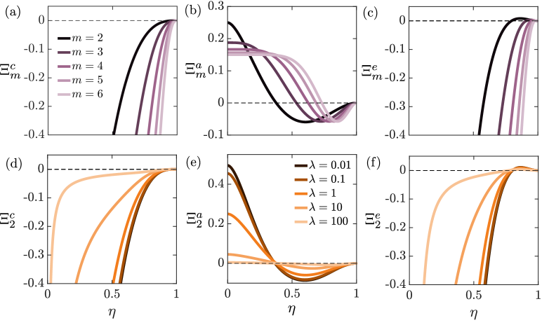
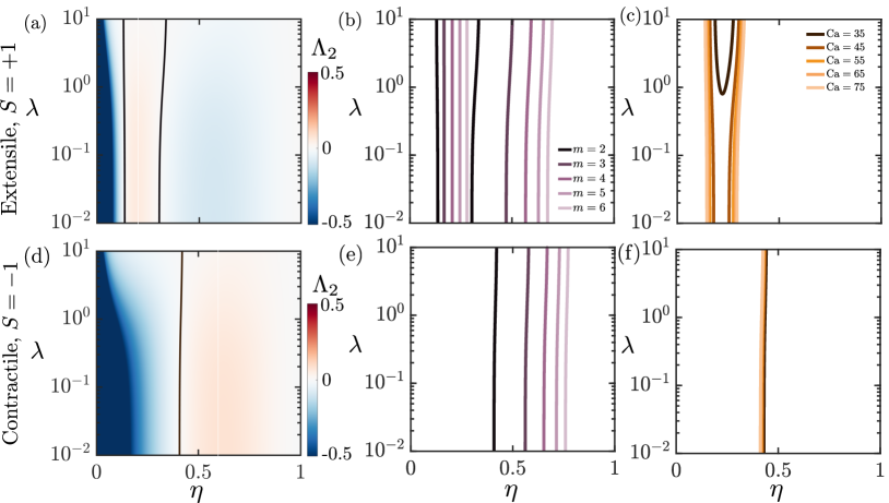
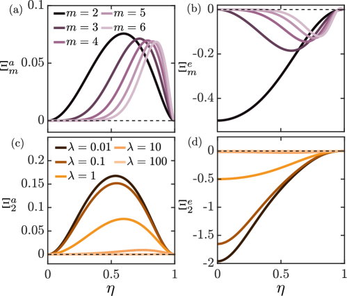
The dependence of , and on , and is illustrated in Fig. 4, where panels (a), (b) and (c) show the dependence on drop size for distinct modes , and panels (d), (e) and (f) show the effect of viscosity ratio for mode . Capillary stresses always favor a circular drop and are therefore stabilizing, especially in the case of small drops and high wavenumbers; this damping effect of surface tension is most pronounced in low-viscosity drops. In the case of extensile systems, activity is destabilizing in the case of drops of small to intermediate sizes (), and stabilizing for large drops, and the range of unstable sizes increases with ; these trends are reversed for contractile systems. In both cases, low-viscosity drops are the ones that are most affected by activity (largest magnitude of the growth rate), and the limit of high-viscosity drops () is neutrally stable. On the other hand, nematic elasticity always stabilizes small to medium-sized drops, but weakly destabilizes large drops. These effects are most pronounced at low wavenumbers and low viscosity ratios.
Figure 5(a) shows a color plot of the total growth rate corresponding to mode in the parameter space, for an extensile system. The system is stable at lower values of the radius ratio () followed by a range of unstable droplet sizes , and eventually regains stability at larger values of . This behavior can be explained as follows: at lower values of , capillary and elastic stresses dominate and are stabilizing; as increases, their effect weakens and the system becomes unstable as a result of active stresses; at larger values of , active stresses become stabilizing leading to a negative growth rate. The marginal stability curve demarcating these regimes is only weakly affected by the viscosity ratio. As shown in Fig. 5(b), increasing the mode number tends to increase the size of the unstable region. Expectedly, decreasing the capillary number tends to stabilize the system across all drop sizes, especially at low viscosity ratios as illustrated in Fig. 5(c). The contractile case is analyzed similarly in Fig. 5(d,e,f). In this case, alternating regions of stable and unstable growth rates are not observed; rather, a single stable region at low values of gives way to an unstable region in the case of larger drops.
As done previously for the translational mode, we examine the bulk and interfacial active and elastic stresses emerging at linear order due to the deformation of the drop. When , the bulk active and elastic force densities have components
| (64) |
and
| (65) |
They are plotted in Fig. 6 for mode and , along with the first-order surface tractions acting on the interface. The fields shown in the figure suggest a destabilizing effect of bulk stresses and a stabilizing effect of surface tractions, both elastic and active (in the extensile case). The interplay of these forces, together with hydrodynamic stresses whose distribution is not explicitly known, gives rise to the trends found in Figs. 4 and 5.
IV The inverted problem: Active nematic drop within a passive layer
In this section, we extend our theory to analyze the inverse scenario, namely, the stability of an active nematic droplet surrounded by a passive viscous layer. Much of the theoretical formulation presented above remains unchanged, with the difference that active and elastic stresses are now exerted inside the drop (). As a result, we do not present the full theory again, but instead only highlight places where differences arise.
IV.1 Governing equations, boundary conditions and non-dimensionalization
Governing equations (1)–(8) still apply, the only difference being that the active and elastic stresses of Eqs. (6) and (7) are now applied inside the drop. As a result, they are decorated by an overbar and enter the momentum equation (8) instead of (4). The kinematic boundary condition (11) is unchanged, while the dynamic boundary condition, in dimensionless form, becomes:
| (66) |
IV.2 Linear stability analysis
IV.2.1 Base state
In the base state, the nematic field lines inside the drop are also circles centered at the origin, with given by Eq. (18). A topological defect of charge is present at the origin. The base state active and elastic stresses inside the drop are still given by Eq. (19). They induce a pressure field inside the drop that diverges at the location of the defect, while the pressure outside the drop is uniform:
| (67) |
IV.2.2 Domain perturbation and linearized problem
The shape of the drop is once again deformed according to Eq. (23), which results in the boundary condition of Eq. (26) for the perturbation angle at the drop surface. A solution of inside the drop that satisfies this condition while remaining bounded at can be obtained as
| (68) |
Equations (29) and (31) are still valid inside the drop. At linear order, the dynamic boundary condition (66) yields
| (69) |
IV.2.3 Lorentz reciprocal theorem
Application of the Lorentz reciprocal theorem follows the same step as discussed in Sec. III.5 and uses the same auxiliary Newtonian flow problem. Once again, the main difference with Sec. III.5 is that active and elastic stresses now appear inside the drop. As a result, the analog of Eq. (43) has no bulk contribution and reads
| (70) |
Conversely, the analog of Eq. (44) does include a surface integral:
| (71) |
where denotes the interior of the drop in two dimensions. Combining Eqs. (70) and (71) yields the main result
| (72) |
The first term in the contour integral can be simplified as in Eq. (46). Using the linearized dynamic boundary condition (69), the second term simplifies to
| (73) |
Finally, the surface integral on the right-hand side of Eq. (72) can be evaluated as
| (74) | ||||
IV.3 Dispersion relation and growth rates
Inserting Eqs. (46), (73) and (74) into Eq. (72) provides an expression for the growth in the form on Eq. (52), with contributions from capillary, active and elastic stresses that we discuss next.
In the translational mode (), capillary stresses do not play a role and the active and elastic growth rates are
| (75) |
These growth rates are plotted in Fig. 7 vs and . Active stresses are destabilizing in extensile systems and stabilizing in contractile systems, whereas elasticity always resists translation. Both active and elastic effects are most pronounced for small drops and at low viscosity ratios. In extensile systems with finite elasticity, the stability of the system in the parameter space is shown in Fig. 7(c): small drops are all stabilized by elasticity, whereas drops with intermediate size can be unstable under translation as a result of activity.
For deformation modes , the capillary, active and elastic growth rates are expressed as
| (76) | ||||
| (77) | ||||
| (78) |
Equation (76) for the capillary growth rate is the same as (61) and was already analyzed in Fig. 4(a) and (d).
The variation of the active and elastic contributions to the growth rate for deformation modes of increasing wavenumber is shown in Fig. 8(a,b). In extensile systems, activity is destabilizing for all wavenumbers and viscosity ratios, especially for a drop of intermediate to large sizes –. Elasticity, on the other hand, is mostly stabilizing and its effect is most pronounced in smaller drops at low wavenumbers. The effect of viscosity ratio is analyzed in Fig. 8(c,d) for mode , which shows that low viscosity drops are the most affected by both activity and elasticity.
V Conclusions
We have analyzed the linear stability of a passive viscous Newtonian drop immersed in an active nematic liquid crystal in two dimensions. In extensile systems, activity was found to stabilize the translational mode, but to destabilize deformation modes for small to intermediate drop sizes; these findings are reversed in contractile systems. Elasticity has a predominantly stabilizing effect, except in the case of small drops with low viscosity ratios. We also considered the inverted problem of an active nematic drop surrounded by a viscous layer, where extensile stresses were found to be always destabilizing. When active, elastic, and capillary stresses act in concert, complex trends are predicted, with a non-trivial and non-intuitive dependence of the stability results on droplet size and viscosity ratio.
Our model relied on several strong assumptions that may need to be relaxed or improved upon for comparison with specific experimental systems. Specifically, we considered a sharply aligned liquid crystal in the limit of strong nematic relaxation () and with strong anchoring boundary conditions. A consequence of these choices is that the configuration of the nematic is fully determined by the instantaneous geometry of the system and is not directly affected by the viscous flow driven by the various stresses in the bulk of the nematic. If the assumption of strong elasticity is relaxed, additional instabilities can arise that involve spontaneous swirling flows, as has been observed in experiments Woodhouse and Golstein (2012); Ray et al. (2023) and other models Fürthauer et al. (2012); Theillard et al. (2017); the impact of such flows on the stability problem analyzed here in unknown. The potential emergence and role of topological defects is another question of interest: no defects were present in the model analyzed here (except for the defect at the origin in the inverted problem of Sec. IV), but defects may arise in other geometries Chandler and Spagnolie (2024); Neville et al. (2024) and are likely to have an impact on the stability and dynamics. The interaction of multiple droplets suspended in an active nematic is also an open topic of interest.
Our theoretical model may be relevant to a wide range of biological systems. As an example, we highlight the dynamics and self-organization inside the cell nucleus, a highly heterogeneous confined environment involving the coexistence of transcriptionally active euchromatin, thought to behave as a nematic active fluid Bruinsma et al. (2014); Saintillan et al. (2018); Eshghi et al. (2021); Mahajan et al. (2022), with various passive compartments such as transcriptionally silent heterochromatin domains, which are passive and viscoelastic Eshghi et al. (2021), as well as nucleoli, which behave as viscous liquid droplets Caragine et al. (2018). Experimental observations suggest the preferential placement of heterochromatin domains near the nuclear envelope, whereas nucleoli tend to be located in the bulk. While our understanding of the rheological behavior of these various phases and of their physical interactions is in its infancy, models such as ours may provide an useful tool for analyzing and explaining their spatiotemporal organization.
Acknowledgements.
The authors acknowledge financial support from National Science Foundation Grant No. DMS-2153520 (D.S.).Appendix: Auxiliary Newtonian problem
The Stokes equations (37)–(38) lead to the biharmonic equation for the streamfunctions, which translate to an equidimensional differential equation for ,
| (A-1) |
and an identical equation for . The boundary conditions on and are
-
•
the no-slip condition at :
(A-2) -
•
the continuity of velocities at :
(A-3) -
•
the stress balance of Eq. (39) in the radial and azimuthal directions:
(A-4) (A-5) -
•
boundedness of the velocity at the origin .
These boundary conditions can be used to solve for the eight integration constants obtained when integrating (A-1) in both fluid domains. Solution details differ for (translation mode) and (deformation modes).
Translation mode
When , Eq. (A-1) for admits the solution
| (A-6) |
where , , and are dimensionless functions of the viscosity ratio and radius ratio . A similar expression holds for , where to ensure boundedness of the velocity at the origin. Applying boundary conditions (A-2)–(A-5) provides six linear equations for the six unknown coefficients, with the solutions
| (A-7) | |||||
| (A-8) | |||||
| (A-9) |
Deformation modes
When , the expression for reads
| (A-10) |
with a similar expression for in which to ensure boundedness at . As for , applying the boundary conditions yields six equations for the coefficients, which are obtained as
| (A-11) | ||||
| (A-12) | ||||
| (A-13) | ||||
| (A-14) |
| (A-15) | ||||
| (A-16) |
where the prefactor is given by
| (A-17) |
References
- Patteson et al. (2018) A. E. Patteson, A. Gopinath, and P. E. Arratia, “The propagation of active-passive interfaces in bacterial swarms,” Nat. Commun. 9, 5373 (2018).
- Martínez-Calvo et al. (2022) A. Martínez-Calvo, T. Bhattacharjee, R. K. Bay, H. N. Luu, A. M. Hancock, N. S. Wingreen, and S. S. Datta, “Morphological instability and roughening of growing 3D bacterial colonies,” Proc. Natl. Acad. Sci. USA 119, e2208019119 (2022).
- Nürnberg et al. (2011) A. Nürnberg, T. Kitzing, and R. Grosse, “Nucleating actin for invasion,” Nat. Rev. Cancer. 11, 177 (2011).
- Hoshino et al. (2013) D. Hoshino, K. M Branch, and A. M Weaver, “Signaling inputs to invadopodia and podosomes,” J. Cell Sci. 126, 2979–2989 (2013).
- Martin and Parkhurst (2004) P. Martin and S. M. Parkhurst, “Parallels between tissue repair and embryo morphogenesis,” Development 131, 3021–3034 (2004).
- Armengol-Collado et al. (2023) J.-M. Armengol-Collado, L. N. Carenza, J. Eckert, D. Krommydas, and L. Giomi, “Epithelia are multiscale active liquid crystals,” Nat. Phys. 19, 1773–1779 (2023).
- Chu et al. (2017) F.-Y. Chu, S. C. Haley, and A. Zidovska, “On the origin of shape fluctuations of the cell nucleus,” Proc. Natl. Acad. Sci. USA 114, 10338 (2017).
- Mogilner and Manhart (2018) A. Mogilner and A. Manhart, “Intracellular fluid mechanics: Coupling cytoplasmic flow with active cytoskeletal gel,” Annu. Rev. Fluid Mech. 50, 347 (2018).
- Caragine et al. (2018) C. M. Caragine, S. C. Haley, and A. Zidovska, “Surface fluctuations and coalescence of nucleolar droplets in the human cell nucleus,” Phys. Rev. Lett. 121, 148101 (2018).
- Mahajan et al. (2022) A. Mahajan, W. Yan, A. Zidovska, D. Saintillan, and M. J Shelley, “Euchromatin activity enhances segregation and compaction of heterochromatin in the cell nucleus,” Phys. Rev. X 12, 041033 (2022).
- Sanchez et al. (2012) T. Sanchez, D. T. N. Chen, S. J. DeCamp, M. Heymann, and Z. Dogic, “Spontaneous motion in hierarchically assembled active matter,” Nature 491, 431–434 (2012).
- Shelley (2016) M. J. Shelley, “The dynamics of microtubule/motor-protein assemblies in biology and physics,” Annu. Rev. Fluid Mech. 48, 487–506 (2016).
- Adkins et al. (2022) R. Adkins, I. Kolvin, Z. You, S. Witthaus, M. C. Marchetti, and Z. Dogic, “Dynamics of active liquid interfaces,” Science 377, 768–772 (2022).
- Tjhung et al. (2012) E. Tjhung, D. Marenduzzo, and M. E. Cates, “Spontaneous symmetry breaking in active droplets provides a generic route to motility,” Proc. Natl. Acad. Sci. USA 109, 12381–12386 (2012).
- Joanny and Ramaswamy (2012) J. F. Joanny and S. Ramaswamy, “A drop of active matter,” J. Fluid Mech. 705, 46–57 (2012).
- Giomi and DeSimone (2014) L. Giomi and A. DeSimone, “Spontaneous division and motility in active nematic droplets,” Phys. Rev. Lett. 112, 147802 (2014).
- Whitfield et al. (2014) C. A. Whitfield, D. Marenduzzo, R. Voituriez, and R. J. Hawkins, “Active polar fluid flow in finite droplets,” Eur. Phys. J. E 37, 1–15 (2014).
- Khoromskaia and Alexander (2015) D. Khoromskaia and G. P. Alexander, “Motility of active fluid drops on surfaces,” Phys. Rev. E 92, 062311 (2015).
- Young et al. (2021) Y.-N. Young, M. Shelley, and D. Stein, “The many behaviors of deformable active droplets,” MBE 18 (2021).
- Alert (2022) R. Alert, “Fingering instability of active nematic droplets,” J. Phys. A: Math. Theor. 55, 234009 (2022).
- Voituriez et al. (2006) R. Voituriez, J. F. Joanny, and J. Prost, “Generic phase diagram of active polar films,” Phys. Rev. Lett. 96, 028102 (2006).
- Sankararaman and Ramaswamy (2009) S. Sankararaman and S. Ramaswamy, “Instabilities and waves in thin films of living fluids,” Phys. Rev. Lett. 102, 118107 (2009).
- Blow et al. (2017) M. L. Blow, M. Aqil, B. Liebchen, and D. Marenduzzo, “Motility of active nematic films driven by “active anchoring”,” Soft Matter 13, 6137–6144 (2017).
- Alonso-Matilla and Saintillan (2019) R. Alonso-Matilla and D. Saintillan, “Interfacial instabilities in active viscous films,” J. Nonnewton. Fluid Mech. 269, 57–64 (2019).
- Freund (2023) J. B. Freund, “Object transport by a confined active suspension,” J. Fluid Mech. 960, A16 (2023).
- Freund (2024) J. B. Freund, “Free object in a confined active contractile nematic fluid: Fixed-point and limit-cycle behaviors,” Phys. Rev. Fluids 9, 053302 (2024).
- Fürthauer et al. (2012) S. Fürthauer, M. Neef, S. W. Grill, K. Kruse, and F. Jülicher, “The Taylor–Couette motor: spontaneous flows of active polar fluids between two coaxial cylinders,” New J. Phys. 14, 023001 (2012).
- Chandler and Spagnolie (2024) T. G. J. Chandler and S. E. Spagnolie, “Active nematic response to a deformable body or boundary: elastic deformations and anchoring-induced flow,” arXiv:2409.15617v1 (2024).
- Masoud and Stone (2019) H. Masoud and H. A. Stone, “The reciprocal theorem in fluid dynamics and transport phenomena,” J. Fluid Mech. 879 (2019).
- Ericksen (1961) J. L. Ericksen, “Conservation laws for liquid crystals,” Trans. Soc. Rheol. 5, 23–34 (1961).
- Ericksen (1962) J. L. Ericksen, “Hydrostatic theory of liquid crystals,” Arch. Ration. Mech. Anal. 9, 371–378 (1962).
- Leslie (1968) F. M. Leslie, “Some constitutive equations for liquid crystals,” Arch. Ration. Mech. Anal. 28, 265–283 (1968).
- De Gennes and Prost (1995) P. G. De Gennes and J. Prost, The Physics of Liquid Crystals (Clarendon Press, 1995).
- Gao et al. (2017) T. Gao, M. D. Betterton, A. S. Jhang, and M. J. Shelley, “Analytical structure, dynamics, and coarse graining of a kinetic model of an active fluid,” Phys. Rev. Fluids 2, 093302 (2017).
- Saintillan and Shelley (2013) D. Saintillan and M. J. Shelley, “Active suspensions and their nonlinear models,” C. R. Physique 14, 497–517 (2013).
- Saintillan (2018) D. Saintillan, “Rheology of active fluids,” Annu. Rev. Fluid Mech. 50, 563–592 (2018).
- Woodhouse and Golstein (2012) F. G. Woodhouse and R. E. Golstein, “Spontaneous circulation of confined active suspensions,” Phys. Rev. Lett. 109, 168105 (2012).
- Ray et al. (2023) S. Ray, J. Zhang, and Z. Dogic, “Rectified rotational dynamics of mobile inclusions in two-dimensional active nematics,” Phys. Rev. Lett. 130, 238301 (2023).
- Theillard et al. (2017) M. Theillard, R. Alonso-Matilla, and D. Saintillan, “Geometric control of active collective motion,” Soft Matter 13, 363–375 (2017).
- Neville et al. (2024) L. Neville, J. Eggers, and T. B. Liverpool, “Controlling wall–particle interactions with activity,” Soft Matter 20, 8395–8406 (2024).
- Bruinsma et al. (2014) R. Bruinsma, A. Y. Grosberg, Y. Rabin, and A. Zidovska, “Chromatin hydrodynamics,” Biophys. J. 106, 1871–1881 (2014).
- Saintillan et al. (2018) D. Saintillan, M. J. Shelley, and A. Zidovska, “Extensile motor activity drives coherent motions in a model of interphase chromatin,” Proc. Natl. Acad. Sci. USA 115, 11442–11447 (2018).
- Eshghi et al. (2021) I. Eshghi, J. A. Eaton, and A. Zidovska, “Interphase chromatin undergoes a local sol-gel transition upon cell differentiation,” Phys. Rev. Lett. 126, 228101 (2021).