Stability Guarantees for Feature Attributions with Multiplicative Smoothing

We first present explainable models as a formalism for rigorously studying explanations. Let $\mathcal{X}=\mathbb{R}^{n}$ be the space of inputs, a classifier $f:\mathcal{X}\to[0,1]^{m}$ maps inputs $x\in\mathcal{X}$ to $m$ class probabilities that sum to $1$, where the class of $f(x)\in[0,1]^{m}$ is taken to be the largest coordinate. Similarly, an explanation method $\varphi:\mathcal{X}\to\{0,1\}^{n}$ maps an input $x\in\mathcal{X}$ to an explanation $\varphi(x)\in\{0,1\}^{n}$ that indicates which features are considered explanatory for the prediction $f(x)$. In particular, we may pick and adapt $\varphi$ from among a selection of existing feature attribution methods like LIME [6], SHAP [7], and many others [5, 8, 23, 24, 25], wherein $\varphi$ may be thought of as a top-$k$ feature selector. Note that the selection of input features necessarily depends on the explanation method executing or analyzing the model, and so it makes sense to jointly study the model and explanation method: given a classifier $f$ and explanation method $\varphi$, we call the pairing $\langle f,\varphi\rangle$ an explainable model. Given some $x\in\mathcal{X}$, the explainable model $\langle f,\varphi\rangle$ maps $x$ to both a prediction and explanation. We show this in Figure 2, where $\langle f,\varphi\rangle(x)\in[0,1]^{m}\times\{0,1\}^{n}$ pairs the class probabilities and the feature attribution.

For an input $x\in\mathcal{X}$, we will evaluate the quality of the binary feature attribution $\varphi(x)$ through its masking on $x$. That is, we will study the behavior of $f$ on the masked input $x\odot\varphi(x)\in\mathcal{X}$, where $\odot$ is the element-wise vector product. To do this, we define a notion of prediction equivalence: for two $x,x^{\prime}\in\mathcal{X}$, we write $f(x)\cong f(x^{\prime})$ to mean that $f(x)$ and $f(x^{\prime})$ yield the same class. This allows us to formalize the intuition that an explanation $\varphi(x)$ should recover the prediction of $x$ under $f$.

Evaluating $f$ on $x\odot\varphi(x)$ this way lets us apply the model as-is and therefore avoids the challenge of constructing a surrogate model that is accurate to the original [26]. Moreover, this approach is reasonable, especially in domains like vision — where one intuitively expects that a masked image retaining only the important features should induce the intended prediction. Indeed, architectures like Vision Transformer [9] can maintain high accuracy with only a fraction of the image present [27].

Particularly, we would like for $\langle f,\varphi\rangle$ to generate explanations that are stable and concise (i.e. sparse). The former is our central guarantee and is ensured through smoothing. The latter implies that $\varphi(x)$ has few ones entries, and is a desirable property since a good explanation should not contain too much redundant information. However, sparsity is a more difficult property to enforce, as this is contingent on the model having high accuracy with respect to heavily masked inputs. For sparsity, we present a simple heuristic in Section 2.4 and evaluate its effectiveness in Section 4.

Given an explainable model $\langle f,\varphi\rangle$ and some $x\in\mathcal{X}$, stability means that the prediction does not change even if one adds more explanatory features to $\varphi(x)$. For instance, the model-explanation pair in Figure 1 is not stable, as the inclusion of a single feature group (patch) changes the prediction. To formalize this notion of stability, we first introduce a partial ordering: for $\alpha,\alpha^{\prime}\in\{0,1\}^{n}$, we write $\alpha\succeq\alpha^{\prime}$ iff $\alpha_{i}\geq\alpha_{i}^{\prime}$ for all $i=1,\ldots,n$. That is, $\alpha\succeq\alpha^{\prime}$ iff $\alpha$ includes all the features selected by $\alpha^{\prime}$.

Note that the constant explanation $\varphi(x)=\mathbf{1}$, the vector of ones, makes $\langle f,\varphi\rangle$ trivially stable at every $x\in\mathcal{X}$, though this is not a concise explanation. Additionally, stability at $x$ implies consistency at $x$.

Unfortunately, stability is a difficult property to enforce in general, as it requires that $f$ satisfy a monotone-like behavior with respect to feature inclusion — which is especially challenging for complex models like neural networks. Checking stability without additional assumptions on $f$ is also hard: if $k=\lVert\varphi(x)\rVert_{1}$ is the number of ones in $\varphi(x)$, then there are $2^{n-k}$ possible $\alpha\succeq\varphi(x)$ to check. This large space of possible $\alpha\succeq\varphi(x)$ motivates us to examine instead relaxations of stability. We introduce lower and upper relaxations of stability below.

Incremental stability is the lower relaxation since it considers the case where the mask $\alpha$ has only a few features more than $\varphi(x)$. For instance, if one can probably add up to $r$ features to a masked $x\odot\varphi(x)$ without altering the prediction, then $\langle f,\varphi\rangle$ would be incrementally stable at $x$ with radius $r$. We next introduce the upper relaxation that we call decremental stability.

Decremental stability is a subtractive form of stability, in contrast to the additive nature of incremental stability. Particularly, decremental stability considers the case where $\alpha$ has much more features than $\varphi(x)$. If one can provably remove up to $r$ non-explanatory features from the full $x$ without altering the prediction, then $\langle f,\varphi\rangle$ is decrementally stable at $x$ with radius $r$. Note also that decremental stability necessarily entails consistency of $\langle f,\varphi\rangle$, but for simplicity of definitions, we do not enforce this for incremental stability. Furthermore, observe that for a sufficiently large radius of $r=\lceil(n-\lVert\varphi(x)\rVert_{1})/2\rceil$, incremental and decremental stability together imply stability.

If $f:\mathcal{X}\to[0,1]^{m}$ is Lipschitz with respect to the masking of features, then we can guarantee relaxed stability properties for the explainable model $\langle f,\varphi\rangle$. In particular, we require for all $x\in\mathcal{X}$ that $f(x\odot\alpha)$ is Lipschitz with respect to the mask $\alpha\in\{0,1\}^{n}$. This then allows us to establish our main result (Theorem 3.3), which we preview below in Remark 2.6.

Observe that Lipschitz smoothness is, in fact, a stronger assumption than necessary, as besides $\alpha\succeq\varphi(x)$, it also imposes guarantees on $\alpha\preceq\varphi(x)$. Nevertheless, Lipschitz smoothness is one of the few classes of properties that can be guaranteed and analyzed at scale on arbitrary models [22, 28].

Most existing feature attribution methods assign a real-valued score to feature importance, rather than a binary value. We therefore need to convert this to a binary-valued method for use with a stable explainable model. Let $\psi:\mathcal{X}\to\mathbb{R}^{n}$ be such a continuous-valued method like LIME [6] or SHAP [7], and fix some desired incremental stability radius $r_{\mathrm{inc}}$ and decremental stability radius $r_{\mathrm{dec}}$. Given some $x\in\mathcal{X}$ a simple construction for binary $\varphi(x)\in\{0,1\}^{n}$ is described next.

Note that the above method of constructing $\varphi(x)$ does not impose sparsity guarantees in the way that we may guarantee stability through Lipschitz smoothness. Instead, the ordering from a continuous-valued $\psi(x)$ serves as a greedy heuristic for constructing $\varphi(x)$. We show in Section 4 that some feature attributions (e.g., SHAP [7]) tend to yield sparser selections on average compared to others (e.g., Vanilla Gradient Saliency [5]).

Our key insight is that randomly dropping (i.e., zeroing) features will attain the desired smoothness. In particular, we uniformly drop features with probability $1-\lambda$ by sampling binary masks $s\in\{0,1\}^{n}$ from some distribution $\mathcal{D}$ where each coordinate is distributed as $\mathrm{Pr}[s_{i}=1]=\lambda$. Then define $f$ as:

where $\mathcal{B}(\lambda)$ is the Beronulli distribution with parameter $\lambda\in[0,1]$. We give an overview of evaluating $f(x)$ in Figure 3. Importantly, our main results on smoothness (Theorem 3.2) and stability (Theorem 3.3) hold provided each coordinate of $\mathcal{D}$ is marginally Bernoulli with parameter $\lambda$, and so we avoid fixing a particular choice for now. However, it will be easy to intuit the exposition with $\mathcal{D}=\mathcal{B}^{n}(\lambda)$, the coordinate-wise i.i.d. Bernoulli distribution with parameter $\lambda$.

We can equivalently parametrize $f$ using the mapping $g(x,\alpha)=f(x\odot\alpha)$, where it follows that:

Note that one could have alternatively first defined $g$ and then $f$ due to the identity $g(x,\mathbf{1})=f(x)$. We require that the relationship between $f$ and $g$ follows an identity that we call masking equivalence:

This follows by the definition of $g$, and the relevance to stability is this: if masking equivalence holds, then we can rewrite stability properties involving $f$ in terms of $g$’s second parameter as follows:

where incremental and decremental stability may be analogously defined. This translation is useful, as we will prove that $g$ is $\lambda$-Lipschitz in its second parameter (Theorem 3.2), which then allows us to establish the desired stability properties (Theorem 3.3).

Since many choices are valid, we have not given an explicit construction for $\mathcal{D}$. Rather, so long as each coordinate of $s\sim\mathcal{D}$ obeys $s_{i}\sim\mathcal{B}(\lambda)$ then the Lipschitz properties for $g$ follow. The implication here is that although simple distributions like $\mathcal{B}^{n}(\lambda)$ suffice for $\mathcal{D}$, they may not be sample efficient. We show in Section 3.3 how to exploit a structured statistical dependence in order to reduce the sample complexity of computing MuS.

Importantly, we are motivated to develop MuS because standard smoothing techniques, namely additive smoothing [21, 22], may fail to satisfy masking equivalence. Additive smoothing is by far the most popular smoothing technique and differs from our scheme (3) in how noise is applied, where let $\mathcal{D}_{\mathrm{add}}$ and $\mathcal{D}_{\mathrm{mult}}$ be any two distributions on $\mathbb{R}^{n}$:

Particularly, additive smoothing has counterexamples for masking equivalence.

Intuitively, this occurs because additive smoothing primarily applies noise by perturbing feature values, rather than completely masking them. As such, there might be “information leakage” when non-explanatory bits of $\alpha$ are changed into non-zero values. This then causes each sample of $h(x\odot\tilde{\alpha})$ within $g(x,\alpha)$ to observe more features of $x$ than it would have been able to otherwise.

Our core technical result is in showing that $f$ as defined in (2) is Lipschitz to the masking of features. We present MuS in terms of $g$, where it is parametric with respect to the distribution $\mathcal{D}$: so long as $\mathcal{D}$ satisfies a coordinate-wise Bernoulli condition, then it is usable with MuS.

The strength of this result is in its weak assumptions. First, the theorem applies to any model $h$ and input $x\in\mathcal{X}$. It further suffices that each coordinate is distributed as $s_{i}\sim\mathcal{B}(\lambda)$, and we emphasize that statistical independence between different $s_{i},s_{j}$ is not assumed. This allows us to construct $\mathcal{D}$ with structured dependence in Section 3.3, such that we may exactly and efficiently evaluate $g(x,\alpha)$ at a sample complexity of $N\ll 2^{n}$. A low sample complexity is important for making MuS practically usable, as otherwise, one must settle for the expected value subject to probabilistic guarantees. For instance, simpler distributions like $\mathcal{B}^{n}(\lambda)$ do satisfy the requirements of Theorem 3.2 — but costs $2^{n}$ samples because of coordinate-wise independence. Whatever choice of $\mathcal{D}$, one can guarantee stability so long as $g$ is Lipschitz in its second argument.

Note that it is only in the case where the radius $\geq 1$ that non-trivial stability guarantees exist. Because each $g_{k}$ has range in $[0,1]$, this means that a Lipschitz constant of $\lambda\leq 1/2$ is necessary to attain at least one radius of stability. We present in Appendix A.2 some extensions to MuS that allow one to achieve higher coverage of features.

We now present $\mathcal{L}_{qv}(\lambda)$, a distribution on $\{0,1\}^{n}$ that allows for efficient and exact evaluation of a MuS-smoothed classifier. Our construction is an adaption of [28] from uniform to Bernoulli noise, where the primary insight is that one can parametrize $n$-dimensional noise using a single dimension via structured coordinate-wise dependence. In particular, we use a seed vector $v$, where with an integer quantization parameter $q>1$ there will only exist $q$ distinct choices of $s\sim\mathcal{L}_{qv}(\lambda)$. All the while, we still enforce that any such $s$ is coordinate-wise Bernoulli with $s_{i}\sim\mathcal{B}(\lambda)$. Thus, for a sufficiently small quantization parameter (i.e., $q\ll 2^{n}$), we may tractably enumerate through all $q$ possible choices of $s$ and thereby evaluate a MuS-smoothed model with only $q$ samples.

The seed vector $v$ is the source of our structured coordinate-wise dependence, and the one-dimensional source of randomness $s_{\mathrm{base}}$ is used to generate the $n$-dimensional $s$. Such $s\sim\mathcal{L}_{qv}(\lambda)$ then satisfies the conditions for use in MuS (Theorem 3.2), and this noise allows for an exact evaluation of the smoothed classifier in $q$ samples. We have found $q=64$ to be sufficient in practice and that values as low as $q=16$ also yield good performance. We remark that one drawback is that one may get an unlucky seed $v$, but we have not yet observed this in our experiments.

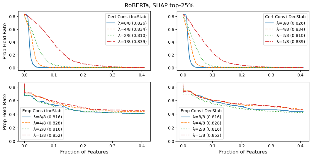
We study how much radius of consistent and incremental (resp. decremental) stability is achieved, and how often. We take an explainable model $\langle f,\varphi\rangle$ where $f$ is Vision Transformer and $\varphi$ is SHAP with top-25% feature selection. We plot the rate at which a property holds (e.g., consistent and incrementally stable with radius $r$) as a function of radius (expressed as a fraction of features $r/n$).

We show our results in Figure 4, where on the left we have the certified guarantees for $N_{\mathrm{cert}}=2000$ samples from ImageNet1K; on the right we have the empirical radii for $N_{\mathrm{emp}}=250$ samples obtained by applying a standard box attack [33] strategy with $q=16$. We observe from the certified results that the decremental stability radii are larger than those of incremental stability. This is reasonable since the base classifier sees much more of the input when analyzing decremental stability and is thus more confident on average, i.e., achieves a larger confidence gap. Moreover, our empirical radii often cover up to half of the input, which suggests that our certified analysis is quite conservative.

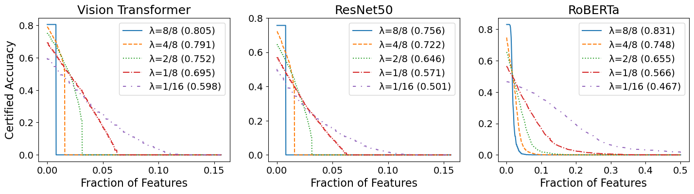
We next investigate how smoothing impacts the classifier accuracy. As $\lambda$ decreases due to more smoothing, the base classifier sees increasingly zeroed-out features — which should hurt accuracy. We took $N=2000$ samples for each classifier on their respective datasets and plotted the certified accuracy vs. radius of decremental stability.

We show the results in Figure 5, where the clean accuracy (in parentheses) decreases with $\lambda$ as expected. This accuracy drop is especially pronounced for ResNet50, and we suspect that the transformer architecture of Vision Transformer and RoBERTa makes them more resilient to the randomized masking of features. Nevertheless, this experiment demonstrates that large models, especially transformers, can tolerate non-trivial noise from MuS while maintaining high accuracy.

Finally, we explore which feature attribution method is best suited to stability guarantees of explainable model $\langle f,\varphi\rangle$. All four methods $\psi\in\{\text{LIME},\text{SHAP},\text{VGrad},\text{IGrad}\}$ are continuous-valued, for which we samples $N=250$ inputs from each model’s respective dataset. For each input $x$, we use the feature importance ranking generated by $\psi(x)$ to iteratively build $\varphi(x)$ in a greedy manner like in Section 2.4. For some $x$, let $k_{x}=\varphi(x)/n$ be the number fraction of features needed for $\langle f,\varphi\rangle$ to be consistent, incrementally stable with radius $1$, and decrementally stable with radius $1$. We then plot the average $k_{x}$ for different methods at $\lambda\in\{1/8,\ldots,4/8\}$ in Figure 6, where note that SHAP tends to require fewer features to achieve the desired properties, while VGrad tends to require more. However, we do not believe these to be decisive results, as many curves are relatively close, especially for Vision Transformer and ResNet50.

References

- [1] Mauricio Reyes, Raphael Meier, Sérgio Pereira, Carlos A Silva, Fried-Michael Dahlweid, Hendrik von Tengg-Kobligk, Ronald M Summers, and Roland Wiest. On the interpretability of artificial intelligence in radiology: challenges and opportunities. Radiology: artificial intelligence, 2(3):e190043, 2020.
- [2] Erico Tjoa and Cuntai Guan. A survey on explainable artificial intelligence (xai): Toward medical xai. IEEE transactions on neural networks and learning systems, 32(11):4793–4813, 2020.
- [3] Sandra Wachter, Brent Mittelstadt, and Chris Russell. Counterfactual explanations without opening the black box: Automated decisions and the gdpr. Harv. JL & Tech., 31:841, 2017.
- [4] Adrien Bibal, Michael Lognoul, Alexandre De Streel, and Benoît Frénay. Legal requirements on explainability in machine learning. Artificial Intelligence and Law, 29:149–169, 2021.
- [5] Karen Simonyan, Andrea Vedaldi, and Andrew Zisserman. Deep inside convolutional networks: Visualising image classification models and saliency maps. arXiv preprint arXiv:1312.6034, 2013.
- [6] Marco Tulio Ribeiro, Sameer Singh, and Carlos Guestrin. " why should i trust you?" explaining the predictions of any classifier. In Proceedings of the 22nd ACM SIGKDD international conference on knowledge discovery and data mining, pages 1135–1144, 2016.
- [7] Scott M Lundberg and Su-In Lee. A unified approach to interpreting model predictions. Advances in neural information processing systems, 30, 2017.
- [8] Mukund Sundararajan, Ankur Taly, and Qiqi Yan. Axiomatic attribution for deep networks. In International conference on machine learning, pages 3319–3328. PMLR, 2017.
- [9] Alexey Dosovitskiy, Lucas Beyer, Alexander Kolesnikov, Dirk Weissenborn, Xiaohua Zhai, Thomas Unterthiner, Mostafa Dehghani, Matthias Minderer, Georg Heigold, Sylvain Gelly, et al. An image is worth 16x16 words: Transformers for image recognition at scale. arXiv preprint arXiv:2010.11929, 2020.
- [10] Amirata Ghorbani, Abubakar Abid, and James Zou. Interpretation of neural networks is fragile. In Proceedings of the AAAI conference on artificial intelligence, volume 33, pages 3681–3688, 2019.
- [11] Joseph Paul Cohen, Joseph D. Viviano, Paul Bertin, Paul Morrison, Parsa Torabian, Matteo Guarrera, Matthew P Lungren, Akshay Chaudhari, Rupert Brooks, Mohammad Hashir, and Hadrien Bertrand. TorchXRayVision: A library of chest X-ray datasets and models. In Medical Imaging with Deep Learning, 2022.
- [12] Gavin Brown. A new perspective for information theoretic feature selection. In Artificial intelligence and statistics, pages 49–56. PMLR, 2009.
- [13] Jianbo Chen, Le Song, Martin Wainwright, and Michael Jordan. Learning to explain: An information-theoretic perspective on model interpretation. In International Conference on Machine Learning, pages 883–892. PMLR, 2018.
- [14] Xiaoping Li, Yadi Wang, and Rubén Ruiz. A survey on sparse learning models for feature selection. IEEE transactions on cybernetics, 52(3):1642–1660, 2020.
- [15] Akhilan Boopathy, Sijia Liu, Gaoyuan Zhang, Cynthia Liu, Pin-Yu Chen, Shiyu Chang, and Luca Daniel. Proper network interpretability helps adversarial robustness in classification. In International Conference on Machine Learning, pages 1014–1023. PMLR, 2020.
- [16] Meike Nauta, Jan Trienes, Shreyasi Pathak, Elisa Nguyen, Michelle Peters, Yasmin Schmitt, Jörg Schlötterer, Maurice van Keulen, and Christin Seifert. From anecdotal evidence to quantitative evaluation methods: A systematic review on evaluating explainable ai. arXiv preprint arXiv:2201.08164, 2022.
- [17] L.S. Shapley. A value for n-person games. Contributions to the Theory of Games, pages 307–317, 1953.
- [18] Yilun Zhou, Serena Booth, Marco Tulio Ribeiro, and Julie Shah. Do feature attribution methods correctly attribute features? In Proceedings of the AAAI Conference on Artificial Intelligence, volume 36, pages 9623–9633, 2022.
- [19] Alon Jacovi and Yoav Goldberg. Towards faithfully interpretable nlp systems: How should we define and evaluate faithfulness? In Proceedings of the 58th Annual Meeting of the Association for Computational Linguistics, pages 4198–4205, 2020.
- [20] Jundong Li, Kewei Cheng, Suhang Wang, Fred Morstatter, Robert P Trevino, Jiliang Tang, and Huan Liu. Feature selection: A data perspective. ACM computing surveys (CSUR), 50(6):1–45, 2017.
- [21] Jeremy Cohen, Elan Rosenfeld, and Zico Kolter. Certified adversarial robustness via randomized smoothing. In International Conference on Machine Learning, pages 1310–1320. PMLR, 2019.
- [22] Greg Yang, Tony Duan, J Edward Hu, Hadi Salman, Ilya Razenshteyn, and Jerry Li. Randomized smoothing of all shapes and sizes. In International Conference on Machine Learning, pages 10693–10705. PMLR, 2020.
- [23] Daniel Smilkov, Nikhil Thorat, Been Kim, Fernanda Viégas, and Martin Wattenberg. Smoothgrad: removing noise by adding noise. arXiv preprint arXiv:1706.03825, 2017.
- [24] Mukund Sundararajan and Amir Najmi. The many shapley values for model explanation. In International conference on machine learning, pages 9269–9278. PMLR, 2020.
- [25] Yongchan Kwon and James Zou. Weightedshap: analyzing and improving shapley based feature attributions. arXiv preprint arXiv:2209.13429, 2022.
- [26] Reza Alizadeh, Janet K Allen, and Farrokh Mistree. Managing computational complexity using surrogate models: a critical review. Research in Engineering Design, 31:275–298, 2020.
- [27] Hadi Salman, Saachi Jain, Eric Wong, and Aleksander Madry. Certified patch robustness via smoothed vision transformers. In Proceedings of the IEEE/CVF Conference on Computer Vision and Pattern Recognition, pages 15137–15147, 2022.
- [28] Alexander J Levine and Soheil Feizi. Improved, deterministic smoothing for l_1 certified robustness. In International Conference on Machine Learning, pages 6254–6264. PMLR, 2021.
- [29] Kaiming He, Xiangyu Zhang, Shaoqing Ren, and Jian Sun. Deep residual learning for image recognition. In Proceedings of the IEEE conference on computer vision and pattern recognition, pages 770–778, 2016.
- [30] Yinhan Liu, Myle Ott, Naman Goyal, Jingfei Du, Mandar Joshi, Danqi Chen, Omer Levy, Mike Lewis, Luke Zettlemoyer, and Veselin Stoyanov. Roberta: A robustly optimized bert pretraining approach. arXiv preprint arXiv:1907.11692, 2019.
- [31] Olga Russakovsky, Jia Deng, Hao Su, Jonathan Krause, Sanjeev Satheesh, Sean Ma, Zhiheng Huang, Andrej Karpathy, Aditya Khosla, Michael Bernstein, et al. Imagenet large scale visual recognition challenge. International journal of computer vision, 115:211–252, 2015.
- [32] Francesco Barbieri, Jose Camacho-Collados, Leonardo Neves, and Luis Espinosa-Anke. Tweeteval: Unified benchmark and comparative evaluation for tweet classification. arXiv preprint arXiv:2010.12421, 2020.
- [33] Pin-Yu Chen, Huan Zhang, Yash Sharma, Jinfeng Yi, and Cho-Jui Hsieh. Zoo: Zeroth order optimization based black-box attacks to deep neural networks without training substitute models. In Proceedings of the 10th ACM workshop on artificial intelligence and security, pages 15–26, 2017.
- [34] Nadia Burkart and Marco F Huber. A survey on the explainability of supervised machine learning. Journal of Artificial Intelligence Research, 70:245–317, 2021.
- [35] Jianlong Zhou, Amir H Gandomi, Fang Chen, and Andreas Holzinger. Evaluating the quality of machine learning explanations: A survey on methods and metrics. Electronics, 10(5):593, 2021.
- [36] Qing Lyu, Marianna Apidianaki, and Chris Callison-Burch. Towards faithful model explanation in nlp: A survey. arXiv preprint arXiv:2209.11326, 2022.
- [37] Xuhong Li, Haoyi Xiong, Xingjian Li, Xuanyu Wu, Xiao Zhang, Ji Liu, Jiang Bian, and Dejing Dou. Interpretable deep learning: Interpretation, interpretability, trustworthiness, and beyond. Knowledge and Information Systems, 64(12):3197–3234, 2022.
- [38] Rishi Bommasani, Drew A Hudson, Ehsan Adeli, Russ Altman, Simran Arora, Sydney von Arx, Michael S Bernstein, Jeannette Bohg, Antoine Bosselut, Emma Brunskill, et al. On the opportunities and risks of foundation models. arXiv preprint arXiv:2108.07258, 2021.
- [39] Ramprasaath R Selvaraju, Michael Cogswell, Abhishek Das, Ramakrishna Vedantam, Devi Parikh, and Dhruv Batra. Grad-cam: Visual explanations from deep networks via gradient-based localization. In Proceedings of the IEEE international conference on computer vision, pages 618–626, 2017.
- [40] Matthew D Zeiler and Rob Fergus. Visualizing and understanding convolutional networks. In Computer Vision–ECCV 2014: 13th European Conference, Zurich, Switzerland, September 6-12, 2014, Proceedings, Part I 13, pages 818–833. Springer, 2014.
- [41] Daniel D Lundstrom, Tianjian Huang, and Meisam Razaviyayn. A rigorous study of integrated gradients method and extensions to internal neuron attributions. In International Conference on Machine Learning, pages 14485–14508. PMLR, 2022.
- [42] Dylan Slack, Anna Hilgard, Sameer Singh, and Himabindu Lakkaraju. Reliable post hoc explanations: Modeling uncertainty in explainability. Advances in neural information processing systems, 34:9391–9404, 2021.
- [43] Tessa Han, Suraj Srinivas, and Himabindu Lakkaraju. Which explanation should i choose? a function approximation perspective to characterizing post hoc explanations. arXiv preprint arXiv:2206.01254, 2022.
- [44] Guy Blanc, Jane Lange, and Li-Yang Tan. Provably efficient, succinct, and precise explanations. Advances in Neural Information Processing Systems, 34:6129–6141, 2021.
- [45] Julius Adebayo, Justin Gilmer, Michael Muelly, Ian Goodfellow, Moritz Hardt, and Been Kim. Sanity checks for saliency maps. Advances in neural information processing systems, 31, 2018.
- [46] Sara Hooker, Dumitru Erhan, Pieter-Jan Kindermans, and Been Kim. A benchmark for interpretability methods in deep neural networks. Advances in neural information processing systems, 32, 2019.
- [47] Jay DeYoung, Sarthak Jain, Nazneen Fatema Rajani, Eric Lehman, Caiming Xiong, Richard Socher, and Byron C Wallace. Eraser: A benchmark to evaluate rationalized nlp models. arXiv preprint arXiv:1911.03429, 2019.
- [48] Jasmijn Bastings, Sebastian Ebert, Polina Zablotskaia, Anders Sandholm, and Katja Filippova. " will you find these shortcuts?" a protocol for evaluating the faithfulness of input salience methods for text classification. arXiv preprint arXiv:2111.07367, 2021.
- [49] Yao Rong, Tobias Leemann, Vadim Borisov, Gjergji Kasneci, and Enkelejda Kasneci. A consistent and efficient evaluation strategy for attribution methods. arXiv preprint arXiv:2202.00449, 2022.
- [50] Yilun Zhou and Julie Shah. The solvability of interpretability evaluation metrics. arXiv preprint arXiv:2205.08696, 2022.
- [51] Julius Adebayo, Michael Muelly, Harold Abelson, and Been Kim. Post hoc explanations may be ineffective for detecting unknown spurious correlation. In International Conference on Learning Representations, 2022.
- [52] Mengjiao Yang and Been Kim. Benchmarking attribution methods with relative feature importance. arXiv preprint arXiv:1907.09701, 2019.
- [53] Pieter-Jan Kindermans, Sara Hooker, Julius Adebayo, Maximilian Alber, Kristof T Schütt, Sven Dähne, Dumitru Erhan, and Been Kim. The (un) reliability of saliency methods. In Explainable AI: Interpreting, Explaining and Visualizing Deep Learning, pages 267–280. Springer, 2019.
- [54] Dylan Slack, Anna Hilgard, Himabindu Lakkaraju, and Sameer Singh. Counterfactual explanations can be manipulated. Advances in neural information processing systems, 34:62–75, 2021.
- [55] Adam Ivankay, Ivan Girardi, Chiara Marchiori, and Pascal Frossard. Fooling explanations in text classifiers. arXiv preprint arXiv:2206.03178, 2022.
- [56] Blair Bilodeau, Natasha Jaques, Pang Wei Koh, and Been Kim. Impossibility theorems for feature attribution. arXiv preprint arXiv:2212.11870, 2022.
- [57] Pang Wei Koh and Percy Liang. Understanding black-box predictions via influence functions. In International conference on machine learning, pages 1885–1894. PMLR, 2017.
- [58] Andrew Ilyas, Sung Min Park, Logan Engstrom, Guillaume Leclerc, and Aleksander Madry. Datamodels: Predicting predictions from training data. arXiv preprint arXiv:2202.00622, 2022.
- [59] Sung Min Park, Kristian Georgiev, Andrew Ilyas, Guillaume Leclerc, and Aleksander Madry. Trak: Attributing model behavior at scale. arXiv preprint arXiv:2303.14186, 2023.
- [60] Shahaf Bassan and Guy Katz. Towards formal xai: Formally approximate minimal explanations of neural networks. In International Conference on Tools and Algorithms for the Construction and Analysis of Systems, pages 187–207. Springer, 2023.
- [61] Diederik P Kingma and Jimmy Ba. Adam: A method for stochastic optimization. arXiv preprint arXiv:1412.6980, 2014.
- [62] Alexey Kurakin, Ian Goodfellow, and Samy Bengio. Adversarial machine learning at scale. arXiv preprint arXiv:1611.01236, 2016.
- [63] Logan Engstrom, Andrew Ilyas, Hadi Salman, Shibani Santurkar, and Dimitris Tsipras. Robustness (python library), 2019.
Appendix A Proofs and Theoretical Discussions
In this Section, we present the proofs of our main results and some extensions to MuS.
A.1 Proofs of Main Results
A.1.1 Proof of Theorem 3.2
Proof.
By linearity, we have:
so it suffices to analyze an arbitrary term by fixing some . Consider any , let , and define . Observe that exactly when and . Since , we thus have , and applying the union bound:
and so:
Note that , and so
Thus, is -Lipschitz in the norm. ∎
A.1.2 Proof of Theorem 3.3
We first show incremental stability. Consider any , then by masking equivalence:
and let be the top-two class probabilities of as defined in (1). By Theorem 3.2, both are Lipschitz in their second parameter, and so for all :
Observe that if is sufficiently close to , i.e.:
then the top-class index of and are the same. This means that and thus , thus proving incremental stability with radius .
The decremental stability case is similar, except we replace with . ∎
A.2 Some Basic Extensions
Below, we present some extensions to MuS that help increase the fraction of the input to which we can guarantee stability.
A.2.1 Feature Grouping
We have so far assumed that , but sometimes it may be desirable to group features together, e.g., color channels of the same pixel. Our results also hold for more general , where for such and we lift as
All of our proofs are identical under this construction, with the exception of the dimensionalities of terms like . Figure 1 gives an example of feature grouping.
Appendix B All Experiments
Models, Datasets, and Explanation Methods
We evaluate on two vision models (Vision Transformer [9] and ResNet50 [29]) and one language model (RoBERTa [30]). For the vision dataset, we use ImageNet1K [31]; for the language dataset, we use TweetEval [32] sentiment analysis. We use four explanation methods in SHAP [7], LIME [6], Integrated Gradients (IGrad) [8], and Vanilla Gradient Saliency (VGrad) [5]; where we take as the top- weighted features.
Training Details
We used Adam [61] as our optimizer with default parameters and a learning rate of for epochs. Because we consider and , there are a total of different models for most experiments. To train with a particular : for each training input , we generate two random maskings — one where of the features are zeroed and one where of the features are zeroed. This additional zeroing is to account for the fact that inputs to a smoothed model will be subject to masking by as well as , where the scaling factor of is informed by our prior experience about the size of a stable explanation.
Miscellaneous Preprocessing
For images in ImageNet1K we use feature grouping (Section A.2.1) to group the dimensional image into patches of size , such that there remains feature groups. Each feature of a feature group then receives the same value of noise during smoothing. We report radii of stability as a fraction of the feature groups covered. For example, if at some input from ImageNet1K, we get an incremental stability radius of , then we report as the fraction of features up to which we are guaranteed to be stable. This is especially amenable to evaluating RoBERTa on TweetEval where inputs do not have uniform token lengths, i.e., do not have uniform feature dimensions. In all of our experiments, we use the quantized noise as in Section 3.3 with a quantization parameter of , with the exception of Appendix B.2 and Appendix B.3. Our experiments are organized as follows:
-
•
(Section B.1) What is the quality of stability guarantees?
(Section B.2) What is the theoretical vs empirical stability that can be guaranteed?
–
We for theoretical guarantees, for empirical guarantees.
(Section B.3) What are the stability-accuracy trade-offs?
We use to study the effect of on MuS-smoothed performance.
(Section B.4) Which explanation method is best?
(Section B.5) Does additive smoothing improve empirical stability?
(Section B.6) Does adversarial training improve empirical stability?
B.1 Quality of Stability Guarantees
Here we study what radii of stability are certifiable, and how often these can be achieved with different models and explanation methods. We therefore consider explainable models constructed from base models and explanation methods with top- feature selection. We take samples from each model’s respective datasets and compute the following value for each radius:
Plots of incremental stability are on the left; plots of decremental stability are on the right.
B.2 Theoretical vs Empirical
We compare the certifiable theoretical stability guarantees with what is empirically attained via a standard box attack search [33]. This is an extension of Section 4.2, where we now show all models as evaluated with SHAP-top25%. We take with for the certified plots, and with for the empirical plots. This is because box attack is time-intensive.
B.3 Stability-Accuracy Trade-Offs
We study how the accuracy degrades with . We consider a smoothed model constructed from a base classifier and vary . We then take samples from each respective dataset and measure the accuracy of at different radii. We use to mean that attained the correct prediction at , and we plot the following value at each radius :
Below, we show the plots for different quantization parameters of . The plots are identical to that of Figure 5. We see that increasing generally improves the performance of MuS, but at a computational cost since this requires evaluations of .
B.4 Which Explanation Method is the Best?
We first investigate how many features are needed to yield consistent and non-trivially stable explanations, as done by the greedy selection algorithm in Section 2.4. For some , let denote the fraction of features that needs to be consistent, incrementally stable, and decrementally stable with radius . We vary , where recall is needed for non-trivial stability, and use samples to plot the average . This part is identical to Section 4.3.
We next investigate the ability of each method to predict features that lead to high accuracy. Let , mean that the masked input yields the correct prediction. We then plot this accuracy as we vary the top- for different methods , and , using samples.
B.5 Empirical Stability of Additive Smoothing
We now study how well additive smoothing impacts empirical robustness compared to multiplicative smoothing. Although additive smoothing cannot yield theoretical stability guarantees (c.f. Proposition 3.1), we nevertheless investigate its empirical performance. We use explanations generated by SHAP top-25% and use Vision Transformer as our base model . We fine-tuned different variants of Vision Transformer at and used these in two general classes of models: Vision Transformer with multiplicative smoothing, and Vision Transformer with additive smoothing. We call these two and respectively, and define them as follows:
where for multiplicative smoothing, is as in Theorem 3.2. Over samples from ImageNet1K, we check how often incremental stability of radius is obtained, and plot our results in Figure 17 (left). We see that multiplicative smoothing yields better empirical performance than additive smoothing.
B.6 Empirical Stability of Adversarial Training
Similar to Section B.5, we also check how adversarial training [62] affects empirical stability. We consider ResNet50 with different adversarial training setups from the Robustness Python library [63] and compare them to their respective MuS-wrapped variants. As with Section B.5 we take samples from ImageNet1K, and plot our results in Figure 17 (right).
B.7 Discussion
Effect of Smoothing
We observe that smoothing can yield non-trivial stability guarantees, especially for Vision Transformer and RoBERTa, as evidenced in Appendix B.1. We see that smoothing is least detrimental on these two transformer-based architectures, and most negatively impacts the performance of ResNet50. We conjecture that although different training set-ups may improve performance across every category, this still serves to illustrate the general trend.
Theoretical vs Empirical
It is expected that the certifiable radii of stability is more conservative than what is empirically observed. As mentioned in Section 3.2, for each , there is a maximum radius to which stability can be guaranteed, which is an inherent limitation of using confidence gaps and Lipschitz constants as the main theoretical technique. We emphasize that the notion of stability need not be tied to smoothing, though we are currently not aware of other viable approaches.
Why these Explanation Methods?
We chose SHAP, LIME, IGrad, and VGrad from among the large variety of methods available primarily due to their popularity, and because we believe that they are collectively representative of many techniques. In particular, we believe that LIME remains a representative baseline for surrogate model-based explanation methods. SHAP and IGrad are, to our knowledge, the two most well-known families of axiomatic feature attribution methods. Finally, we believe that VGrad is representative of a traditional gradient saliency-based approach.
Which Explanation Method is the Best?
Based on our experiments in Appendix B.4 we see that SHAP generally achieves higher accuracy using the same amount of top- features as other methods. On the other hand, VGrad tends to perform poorly. We remark that there are well-known critiques against the usefulness of saliency-based explanation methods [53].
Appendix C Miscellaneous
Relevance to Other Explanation Methods
Our key theoretical contribution of MuS in Theorem 3.2 is a general-purpose smoothing method that is distinct from standard smoothing techniques, namely additive smoothing. Therefore, MuS is applicable to other problem domains beyond what is studied in this paper and would be useful where small Lipschitz constants with respect to maskings are desirable.
Broader Impacts
Reliable explanations are necessary for making well-informed decisions and are increasingly important as machine learning models are integrated with fields like medicine, law, and business — where the primary users may not be well-versed in the technical limitations of different methods. Formal guarantees are thus important for ensuring the predictability and reliability of complex systems, which then allows users to construct accurate mental models of interaction and behavior. In this work, we study a particular kind of guarantee known as stability, which is key to feature attribution-based explanation methods.