Stability, bifurcation and spikes of stationary solutions in a chemotaxis system with singular sensitivity and logistic source
Abstract
In the current paper, we study stability, bifurcation, and spikes of positive stationary solutions of the following parabolic-elliptic chemotaxis system with singular sensitivity and logistic source,
| (0.1) |
where , , , , are positive constants. Among others, we prove there are and () such that the constant solution of (0.1) is locally stable when and is unstable when , and under some generic condition, for each , a (local) branch of non-constant stationary solutions of (0.1) bifurcates from when passes through , and global extension of the local bifurcation branch is obtained. We also prove that any sequence of non-constant positive stationary solutions of (0.1) with develops spikes at any satisfying . Some numerical analysis is carried out. It is observed numerically that the local bifurcation branch bifurcating from when passes through can be extended to and the stationary solutions on this global bifurcation extension are locally stable when and develop spikes as .
Keywords: Chemotaxis, singular sensitivity, logistic source, stationary solutions, stability, local bifurcation, global bifurcation, spikes.
Mathematics Subject Classification. 35B20, 35B32, 35B40, 35Q92, 92C17, 92D25.
1 Introduction
The current paper is devoted to the study of stability, bifurcation, and spikes of positive stationary solutions of the following parabolic-elliptic chemotaxis system with singular sensitivity and logistic source on a bounded interval complemented with Neumann boundary condition,
| (1.1) |
where and represent the cellular density and chemical concentration at time and location , is the chemotaxis sensitivity coefficient, is the growth rate of the cell population, is the self-limitation rate of the cell population, represents the degradation rate of the chemical signal substance and is the production rate of the chemical signal substance by the cell population.
Chemotaxis models are used to describe the movements of cells or living organisms in response to gradients of some chemical substances. Various chemotaxis systems, also known as Keller-Segel systems, have been widely studied since the pioneering works [16, 17] by Keller and Segel at the beginning of 1970s on the mathematical modeling of the aggregation process of Dictyostelium discoideum.
Consider the following parabolic-elliptic chemotaxis system with singular sensitivity and logistic source in general dimensional setting,
| (1.2) |
where is a bounded smooth domain, and and are positive constants, and are nonnegative constants. A considerable amount of research has been carried out on the global existence and boundedness of positive classical solutions of (1.2).
For example, in the case that and , Biler in [3] proved the global existence of positive solutions of (1.2) when and , or and . Fujie, Winkler, and Yokota in [11] proved the boundedness of globally defined positive solutions of (1.2) when and . Fujie and Senba in [9] proved the global existence and boundedness of classical positive solutions of (1.2) for the case of for any .
In the case that and are positive constants, when Fujie, Winkler, and Yokota in [10] proved that finite-time blow-up does not occur in (1.2), and moreover, if
| (1.3) |
then any globally defined positive solution of (1.2) is bounded. Furthermore, Cao et al. in [5] proved that, if
with the constant depending on , then for any nonnegative initial data , where
| (1.4) |
and satisfying that , the globally defined positive solution of (1.2) converges to as exponentially (see [5, Theorem 1] for details).
Let
| (1.5) |
Recently, Kurt and Shen proved in [22] that classical solutions of (1.2) with initial functions exist globally and stay bounded as time evolves, provided that is not too small and is large relative to (see [22, Theorem 1.2(3)]), which is an interesting biological phenomenon. Moreover, some qualitative properties of (1.2) have been obtained in [23]. For example, assuming that is large relative to , it is shown in [23] that any globally defined positive solution of (1.2) is bounded above and below eventually by some positive constants independent of its initial functions provided that they are not too small.
There are still many interesting dynamical issues to be studied for (1.2). For example, whether any globally defined positive solution of (1.2) is bounded without the assumption that is large relative to ; whether chemotaxis induces non-constant positive stationary solutions and if so, what about the stability of non-constant positive stationary solutions and whether non-constant stationary solutions develop spikes as , etc. Some of those issues are strongly related to the stability and bifurcation of stationary solutions of (1.2).
There are many works on bifurcation and spikes of stationary solutions of various chemotaxis models. For example, local and global bifurcation of constant positive stationary solutions and existence of spiky steady states for chemotaxis models with certain regular sensitivity and with or without logistic source are studied in [15, 18, 19, 20, 21, 31, 32], etc. In particular, consider the following chemotaxis system with regular sensitivity and logistic source,
| (1.6) |
The authors of [20] proved the existence of single boundary spikes to (1.6) when is sufficiently large via the standard Lyapunov–Schmidt reduction. Among others, the authors of [31] carried out bifurcation analysis on (1.6) and obtained the explicit formulas of bifurcation values and small amplitude nonconstant positive solutions.
There are also some studies on bifurcation and spikes of stationary solutions of chemotaxis models with singular sensitivity but without logistic source. For example, in [24] and [34], local and global bifurcation of positive constant solutions and existence of spiky steady states are studied for parabolic-parabolic chemotaxis models with singular sensitivity and without logistic source. It is shown in [24] that positive monotone steady states exist as long as is larger than the first bifurcation value , and that the cell density function forms a spike. The results in [24] apply to (1.1) with . The paper [6] investigated the existence and nonlinear stability of boundary spike-layer solutions of a chemotaxis-consumption type system with logarithmic singular sensitivity in the half space, where the physical zero-flux and Dirichlet boundary conditions are prescribed.
However, there is little study on bifurcations and spiky solutions of (1.1) with . Bifurcation analysis of (1.1) with is of great importance in several aspects. For example, it will show what types of bifurcations may occur in (1.1) as changes and what types of spiky patterns may be developed in (1.1) as . It will discover some intrinsic similarity and/or difference between the singular and regular chemotaxis sensitivities. Note that, considering (1.2), for a positive classical solution to exist globally and stay bounded, it requires that does not become arbitrarily large and (equivalently, ) does not become arbitrarily small on any finite time interval. Consider the following chemotaxis model with regular sensitivity,
| (1.7) |
For a positive classical solution of (1.7) to exist globally and stay bounded, it only requires that does not become arbitrarily large on any finite time interval. It is of great interest to explore intrinsic similarity and difference between singular and regular chemotaxis sensitivity via various analysis.
In this paper, we carry out some bifurcation analysis of (1.1) and some relevant study on stationary solutions of (1.1). In particular, we study the local stability and instability of the positive constant solution of (1.1); bifurcation solutions of (1.1) from the positive constant solution ; properties of non-constant positive stationary solutions; spikes developed by non-constant positive stationary solutions. Among others, we obtain the following results:
- (i)
- (ii)
-
(iii)
The local bifurcation branches can be extended to global branches (see Theorem 4.1 for detail).
- (iv)
- (v)
-
(vi)
A notion of spikes is introduced (see Definition 5.1) and it is proved that any given sequence of non-constant positive stationary solutions of (1.1) with develops spikes as at those satisfying that (see Theorem 5.1) (hence a sequence of non-constant positive stationary solutions of (1.1) with can develop multiple spikes as ).
-
(vii)
Several numerical simulations are carried out and it is observed numerically that the local bifurcation branch in (ii) extends to and the solutions on are locally stable for , stay bounded, and develop spikes as (see Numerical Experiment 2 in section 6 for the case , locally stable boundary spiky solutions are observed in this case, and Numerical Experiment 4 in section 6 for the case , , locally stable spiky solutions with multiple spikes are observed in this case).
The main methods/techniques used and/or developed in this paper for the study of stability, bifurcation, and spikes of positive stationary solutions of (1.1) can be described as follows. We study local stability/instability of positive stationary solutions of (1.1) by general perturbation theory for dynamical systems/differential equations (see [12]). The investigation of local bifurcation of the constant solution of (1.1) is carried out via invariant manifold theory, in particular, center manifold theory, for dynamical systems/differential equations (see [12]). We study the global extension of local bifurcation branches of by the global bifurcation theory developed by Shi and Wang (see [27]). We investigate the development of spikes of non-constant positive stationary solutions of (1.1) via some important properties of positive stationary solutions of (1.1) obtained in this paper, for example, the property (v) stated in the above. This is a novel approach. The above mentioned methods/techniques would be useful for the study of bifurcation and spikes of stationary solutions in other chemotaxis models.
We would like to point out that, many people study the existence of nonconstant positive stationary solutions by applying the local bifurcation theory of Crandall-Rabinowtz (see [7]), which can also be used to study (1.1). In this paper, we employed the center manifold theory as the theoretical framework. The computations associated with this approach are elementary, and by using this method, we obtain several information simultaneously, such as the bifurcation direction and the explicit dependence of the bifurcating solutions on the parameters.
We make the following remarks on the implications of the results obtained in this paper, and some related problems, which are worthy to be studied further.
-
(a)
Some essential difference is observed between the effects of the parameters on the dynamics of (1.1) and (1.6). For example, consider (1.1) and (1.6), and treat as a bifurcation parameter. Let be as in (2.6), that is,
and be as in (2.10), that is,
Let and be as in (2.7) and (2.11), respectively, that is,
Then the constant solution of (1.1) (resp. (1.6)) is locally stable when (resp. ) and unstable when (resp. ), and pitchfork bifurcation occurs in (1.1) (resp. (1.6)) when passes through (resp. ) (see (i), (ii) described in the above and [31]). Hence the larger (resp. ), the less influence of the chemotaxis on the dynamics of (1.1) (resp. (1.6)).
-
(b)
Observe that and depend only on the parameters and in (1.1), and and depend on all the parameters in (1.6). Hence there is some essential difference between the influence of the chemotaxis on the dynamics of (1.1) and (1.6). Mathematically, this difference is due to the following two factors: first, is cancelled in when linearizing (1.1) at the constant solution ; second, can be assumed to be by changing to (after such change of variable, becomes ). Note that
and
Biologically, the difference between and can be interpreted as follows. In the chemotaxis model (1.1) with singular sensitivity, the chemotaxis has less influence on the dynamics of (1.1) if is large or is small, which is natural since large and small prevent from becoming too small as time evolves. In the chemotaxis model (1.6) with regular sensitivity, the chemotaxis has less influence on the dynamics of (1.6) if is small, is large, or is small, which is also natural since small , large , and small prevent from becoming too large as time evolves. The above intrinsic difference between singular and regular chemotaxis sensitivities resulting from the local bifurcation analysis matches in certain sense the difference between the following sufficient conditions for the global existence of positive classical solutions of (1.2) and (1.7): a positive classical solution of (1.2) exists globally if is large relative to and the initial distribution is not too small (see [22, Theorem 1.2(3)]), and a positive classical solution of (1.7) exists globally if is large relative to (see [29, Theorem 2.5]).
-
(c)
Besides rigorous bifurcation analysis near the constant solution , in this paper, we also perform some theoretical as well as numerical analysis of non-constant stationary solutions of (1.1) for and obtain several interesting results (see (iii)-(vii) described in the above). For example, it is observed that, up to a subsequence, as , a sequence of nonconstant stationary solutions of (1.1) develops spikes at any satisfying . It is interesting to further study spiky solutions of (1.1) with , for example, to derive asymptotic expansions of spiky patterns with , to perform some bifurcation analysis around spiky patterns, etc. We leave such questions for future investigation. It should be pointed out that spiky patterns of logistic Keller–Segel models with regular sensitivity has been studied in [18], [20] and [21].
-
(d)
Consider the following two parabolic-parabolic chemotaxis models
(1.8) (1.9) We want to mention that the system (1.8) has very rich spatial-temporal dynamics as demonstrated by the numerical studies in [25]. For example, the authors in [25] numerically demonstrated that the long time dynamics of solutions of (1.8) undergo homogeneous stationary solution, stationary spatial patterns in which multiple-peak patterns develop, spatial-temporal periodic solutions and spatial-temporal irregular solutions which describes a form of spatial-temporal chaos as is increased steadily (see section 5 of [25] for details).
Based on some numerical simulations we performed, complicated dynamics is not observed in (1.9) for various parameter sets. For example, following the same simulations performed in section 5 of [25] and using the same parameter set, we did some numerical simulations for the system (1.9). We did not observe such rich dynamics. Indeed, we only observed homogeneous stationary solution and different peak patterns depending on randomised initial conditions as is increased steadily. Spatial-temporal periodic solutions and spatial-temporal irregular solutions are not observed in (1.9). We also used the parameter sets we used in Section 6.1 and Section 6.2 to simulate the existence of nonconstant solutions for the system (1.9). For the parameter set used in section 6.1, we observed the same phenomenon as demonstrated in section 6.1. For the parameter set in section 6.2, in addition to the phenomenon we observed in section 6.2, we also see the boundary perks. Time-dependent solutions are also not observed. The above numerical simulations indicate that the dynamics of system (1.9) is simpler than that of (1.8). It is certainly important to further explore whether (1.9) exhibits complicated dynamics or not. We also leave this question for future investigation.
The rest of this paper is organized as follows. Section 2 is devoted to the study of the local stability and instability of the constant solution of (1.1). In section 3, we study local bifurcation of and stability of the local bifurcation solutions. The global extension of the local bifurcation is investigated in section 4. Several important properties of non-constant positive stationary solutions of (1.1) are also obtained in section 4. Section 5 is devoted to the study of spiky stationary solutions of (1.1). In the last section, we provide some numerical analysis on the bifurcation and spiky solutions of (1.1).
2 Local stability and instability of the positive constant solution
In this section, we analysis the local stability and instability of the positive constant solution of (1.1) by general perturbation theory.
The following is the main theorem in this section.
Theorem 2.1.
There is depending only on and such that when , the constant solution of (1.1) is locally asymptotically stable with respect to perturbations in and when , is unstable with respect to perturbations in .
Proof.
Recall that for any , (1.1) has a unique globally defined classical solution satisfying that
and is continuous in (see [22, Theorem 1.2]). To prove the local stability of the constant solution , consider the linearized equation of (1.1) at in ,
| (2.1) |
Consider the eigenvalue problem associated with (2.1) in the space ,
| (2.2) |
Let be defined by
where is the unique solution of
| (2.3) |
Note that the spectrum of the operator , denoted by , consists of eigenvalues of (2.2).
Suppose that is an eigenvalue of (2.2) and is a corresponding eigenfunction. Let
Then we have
| (2.4) |
This implies that and for some and , where
| (2.5) |
It then follows that
and is an eigenfunction of associated to the eigenvalue .
It is clear that
Let
| (2.6) |
Then
for Let
| (2.7) |
Then for , all the eigenvalue of (2.2) are negative. Hence is linearly exponentially stable with respect to perturbations in , where is defined as in (1.4). By the general perturbation theory (see [12, Theorem 5.1.1]), is a locally exponentially stable solution of (1.1) with respect to small perturbations in . If , then is linearly unstable with respect to perturbations in . By the general perturbation theory again (see [12, Theorem 5.1.1]), is an unstable solution of (1.1) with respect to small perturbations in . ∎
Remark 2.1.
-
(1)
depends only on and depends only on . Let
We have that is monotone decreasing in for and is monotone increasing in for . Let
be the greatest integer less than or equal to . Then we have the following explicit formula for ,
Note that
Hence
-
(2)
can be any nonnegative integer by properly choosing and . For example, fix , if , then and ; if and , then and ; if , , and , then and .
Remark 2.2.
- (1)
-
(2)
For the case , (1.1) experiences super-critical pitchfork bifurcation when passes through (see Remark 3.1 (1)). It is observed numerically that when , the constant solution of (1.1) is globally stable (see Numerical Experiment 1). But it remains open whether the constant solution of (1.1) is truly globally stable for any .
-
(3)
For the case and , (1.1) experiences sub-critical pitchfork bifurcation when passes through (see Remark 3.1 (2)). It is observed numerically that when and , there are some locally stable nonconstant positive steady-states of (1.1) and hence the constant solution of (1.1) is not globally stable (see Numerical Experiment 3).
-
(4)
For the case , , and , (1.1) also experiences sub-critical pitchfork bifurcation when passes through (see Remark 3.1 (3)). It is also observed numerically that when and , there are some locally stable nonconstant positive steady-states of (1.1) and hence the constant solution of (1.1) is not globally stable (see section 6.4).
Remark 2.3.
Consider (1.6). The linearized equation of (1.6) reads as follows
| (2.8) |
The associated eigenvalue problem to (2.8) reads as
| (2.9) |
We have
is an algebraic simple eigenvalue with being a corresponding eigenfunction. Note that . Let
| (2.10) |
and
| (2.11) |
Then the constant solution is locally asymptotically stable when and unstable when . Detailed bifurcation analysis of (1.6) can be seen in [31] over a one-dimensional bounded region and [14] over a multidimensional bounded domain. It is seen that depends on all the parameters in (1.6) and then depends on all the parameters in (1.6), while defined in (2.7) depends only on and (see Remark 2.1 (1)).
3 Local bifurcation and stability of bifurcating solutions
In this section, we investigate the local bifurcation of (1.1) when passes through , where is given in (2.6).
To state our main results on local bifurcation solutions from the constant solution , we first introduce some notions. For given , let
| (3.1) |
Let
| (3.2) |
and
| (3.3) |
We now state the main results of this section.
Theorem 3.1.
-
(1)
(Pitchfork bifurcation) For given , if and for any , where and are given in (3.3) and (2.5), respectively, then pitchfork bifurcation occurs in (1.1) near when passes through . Moreover, let be the -components of bifurcation solutions of (1.1) for , we have
(3.4) where, for any , is of the form
(3.5) where is given in (3.2), and for any , is of the form
(3.6) -
(2)
(Stability/instability of bifurcation solutions) Assume the conditions in (1). If , then the bifurcation solutions with are unstable.
-
(3)
(Stability/instability of bifurcation solutions) If and , then super-critical pitchfork bifurcation occurs when passes through and the bifurcation solutions with are locally stable. If and , then sub-critical pitchfork bifurcation occurs when passes through and the bifurcation solutions with are unstable.
Remark 3.1.
-
(1)
For the case , we have
Hence supercritical pitchfork bifurcation occurs when passes through .
-
(2)
For the case and , we have
Hence subcritical pitchfork bifurcation occurs for , .
-
(3)
For the case , , , and , we have
Hence subcritical pitchfork bifurcation occurs for , .
Before proving Theorem 3.1, we first make some variable changes. First, let
Then (1.1) becomes
This implies that
that is,
| (3.7) |
Next, let
| (3.8) |
Note that for any , . Hence we have
and
Then the first equation in (3.7) becomes
| (3.9) |
By the second equation in (3.7), we have
| (3.10) |
By (3) and (3.10), we obtain a system of ODEs for , . To be more precise, we first observe that
| (3.11) |
and
| (3.12) |
We also observe that for ,
| (3.13) |
| (3.14) |
| (3.15) |
| (3.16) |
| (3.17) |
| (3.18) |
| (3.19) |
and
| (3.20) |
By (3)-(3), integrating (3) over and then dividing by , we get
| (3.21) |
By (3.10) and (3)-(3), for each , multiplying (3) by and then integrating over , we get
| (3.22) |
where is as in (2.5), and
| (3.23) |
( is given by (3.10)). Combing (3.21) and (3), we have the following system of ODEs for with ,
| (3.24) |
To study the bifurcation of (1.1) near , it then reduces to study the bifurcation of (3.24) from the trivial solutions for .
We now prove Theorem 3.1.
Proof of Theorem 3.1.
(1) Fix . Recall that . We will use center manifold theory to investigate the bifurcation solutions of (3.24) near the zero solution when passes through . To this end, set . We can then write (3.24) as
| (3.25) |
By the assumption in (1), for all . Note that
Then by center manifold theory, for and , there are , and constants () such that
| (3.26) |
and
| (3.27) |
is locally invariant under (3.25). is referred to the center manifold at for (3.25).
In the following, we find the reduced ODE on the center manifold and then study the bifurcation solutions of the reduced ODE. To this end, first, differentiating with respect to and using (3.25), we get on ,
| (3.28) |
for and . On the other hand, we have
| (3.29) |
for and . By (3) and (3), we must have
| (3.30) |
Next, for , , differentiating with respect to and using (3.25), we get on ,
| (3.31) |
for and . On the other hand, we have
| (3.32) |
for and . By (3), when , we have
| (3.33) |
When , we have
| (3.34) |
| (3.35) |
and
| (3.36) |
Now, by (3.30)-(3.36), we have on ,
Therefore, on the center manifold , the dynamics is determined by the following ODE,
| (3.37) |
By (3.1), (3.30), and (3.35), equation (3) can be written as
| (3.38) |
where
Pitchfork bifurcation then occurs in (3.38) near provided that . This proves (1).
(2) Let be such that . If , then and the positive constant solution is linearly unstable. By the general perturbation theory (see [12, Theorem 5.1.3]), any solution with the -component belonging to is linearly unstable for .
(3) If and , then (3.38) experiences super-pitchfork bifurcation near when passes through . This implies that any solution with the -component belonging to is linearly stable for .
If and , then (3.38) experiences sub-pitchfork bifurcation near when passes through . This implies that any solution with the -component belonging to is linearly unstable for . The theorem is thus proved. ∎
4 Global bifurcation and properties of non-constant stationary solutions
In this section, we study the global extension of the local bifurcation branches for and properties of non-constant stationary solutions.
For given , if for all , then there is such that and for . For such , let
and be the connected component of containing . In addition, if , then by Theorem 3.1, pitchfork-type bifurcation occurs in (1.1) near when passes through . In such case, let
Next, we state the main results of this section. The first theorem is on the global bifurcation.
Theorem 4.1 (Global bifurcation).
For given , assume that and for any . Let be the connected component of which contains . Then each of the sets and satisfies one of the following: (i) it is not compact; (ii) it contains a point with ; or (iii) it contains a point , where and , where complements . Moreover, if (resp. ) is not compact, then (resp. ) extends to infinity in the positive direction of .
Remark 4.1.
-
(1)
For any (resp. ) with , (resp. ) for , and (resp. ).
-
(2)
For given , if and super-critical pitchfork bifurcation occurs when passes through , it is observed numerically that the global bifurcation diagram is of the form in Figure 1(a) and the bifurcation solutions are locally stable (see numerical simulations in subsection 6.2), where the red part consists of the u-components of local bifurcation solutions and the blue parts are the global extension of the u-components of local bifurcation solutions.
-
(3)
For given , if and sub-critical pitchfork occurs when passes through , it is observed numerically that the global bifurcation diagram is of the form in Figure 1(b) and the bifurcation solutions with u-components lying in the red and green parts are unstable and the bifurcation solutions with u-components lying in the blue parts are locally stable (see numerical simulations in subsections 6.3 and 6.4), where the red part consists of the u-components of local bifurcation solutions and the green and blue parts are the global extension of the u-components of local bifurcation solutions.


The next two theorems are on the properties of non-constant stationary solutions.
Theorem 4.2 (Properties of non-constant stationary solutions).
Let be a non-constant positive stationary solution of (1.1). Then the following hold.
-
(1)
(4.1) -
(2)
There is a positive constant independent of such that
(4.2) -
(3)
(4.3) and
(4.4) -
(4)
There is such that
(4.5) -
(5)
There is such that
(4.6) -
(6)
If is monotone increasing (respectively, decreasing) on , then is strictly increasing (respectively, decreasing) on .
Remark 4.2.
By Theorem 4.2(3), the set of -components of non-constant positive stationary solutions is bounded in as . By Theorem 4.2(5), the set of -components of non-constant positive stationary solutions is bounded in as and hence is bounded in for some . It remains open whether the set of -components of non-constant positive stationary solutions is bounded in as .
Theorem 4.3 (Properties of non-constant stationary solutions).
Let be a sequence of non-constant positive stationary solutions of (1.1) with and .
-
(1)
If is such that
then there is a constant such that
-
(2)
If is such that
then there is a constant such that
Remark 4.3.
Let be a sequence of non-constant positive stationary solutions of (1.1) with and .
In the following, we prove Theorems 4.1-4.3. We first prove Theorem 4.2 since we need to employ Theorem 4.2 in the proof of Theorem 4.1. Next, we prove Theorem 4.3. We end this section by proving Theorem 4.1.
We first prove Theorem 4.2.
Proof of Theorem 4.2.
(1) We first extend to the following ,
and
It is clear that
| (4.7) |
This implies that
| (4.8) |
Next, let be the solution of
| (4.9) |
Then we also have
| (4.10) |
and
| (4.11) |
This implies that
| (4.12) |
(2) It follows from [11, Lemma 2.1].
(3) First, observe that
| (4.13) |
and . It then follows that
This implies that
and
(4) Integrating the first equation in (4.13) from to and noting that , we get
| (4.14) |
where
By (4.3), there is such that . We then have
| (4.15) |
By (4.1), (4.4), (4.14), and (4.15), there is such that (4.5) holds.
(5) Observe that
By (4.3), (4.4), and a priori estimates for elliptic equations, there is such that (4.6) holds.
(6) Without loss of generality, we assume that is monotone increasing on . Then on . Let . Then is the solution of
| (4.16) |
Since constant, we have constant and . By maximum principle for elliptic equations, we have
This implies that for every . ∎
Next, we prove Theorem 4.3.
Proof of Theorem 4.3.
For simplicity in notation, put
(1) First, By Theorem 4.2,
Without loss of generality, we may then assume that there is such that
Note that
| (4.17) |
We then have converges to weakly in , and is a weak solution of
| (4.18) |
If for a.e. , we have for all . (1) then follows.
In the following, we assume that for a.e. . Then
This implies that
This together with Theorem 4.2(2) implies that there is such that
| (4.19) |
Note that
| (4.20) |
where
By Theorem 4.2, is a bounded sequence on . By (4.19),
This together with (4.20) implies that, for any ,
| (4.21) |
By Fatou’s Lemma, we have
Hence for a.e. , . Therefore, there is such that
Then there is such that exists and
By Fatou’s Lemma again,
Then for a.e. , . Let
For any , there is such that
Then by (4), we have
This implies that for any ,
For any and , there are such that
This implies that
and then
Note that . Let be such that
Then . By (4.18), we have
This implies that
Hence there is such that
| (4.22) |
and then
Note that
Hence . (1) is thus proved.
(2) First, suppose that
By Theorem 4.2(5), without loss of generality, we may assume that there is such that
By the arguments in (1), there is such that
Next, suppose that
By Theorem 4.2(3), is a bounded sequence in . Hence
Then there is such that
The theorem is thus proved. ∎
Finally, we prove Theorem 4.1.
Proof of Theorem 4.1.
When , we have
and
where . It is clear that for any and , is a Fredholm operator. By [27, Theorem 4.4], each of the sets and satisfies one of (i), (ii), (iii) in the statement.
Suppose that satisfies (i), i.e., is not compact. We claim that extends to infinity in the positive direction of . For otherwise, there are such that , and there is no such that . By Theorem 4.2, without loss of generality, we may assume that there are such that
as uniformly in . Then both and are uniformly continuous in . By Theorem 4.2 again, , we must have . This implies that
and then
We then have that is a positive stationary solution of (1.1) with . By the connectness of , we have , which is a contradiction. Therefore, the claim holds.
Similarly, if is not compact, then it extends to infinity in the positive direction of . The theorem is thus proved. ∎
5 Spiky stationary solutions
In this section, we study spiky stationary solutions. We first give the following definition.
Definition 5.1.
Let be positive non-constant stationary solutions of (1.1) with and . We say that develops spikes at as if there are and such that
| (5.1) |
Such is called a spiky point of . If (resp. ), we say that develops boundary spikes (resp. interior spikes).
Remark 5.1.
Let be positive non-constant stationary solutions of (1.1) with and .
-
(1)
The condition (5.1) indicates that for any , is not near a constant function on for .
- (2)
Theorem 5.1 (Spiky stationary solutions).
Let be a sequence of non-constant positive stationary solutions of (1.1) with and .
-
(1)
If satisfies that there is such that
(5.4) then is a spiky point of the sequence . In particular, if satisfies that
(5.5) then is a spiky point of the sequence .
-
(2)
If
(5.6) then there are and such that is a spiky point of the sub-sequence .
-
(3)
If satisfies that
(5.7) then (resp. ) is a boundary spiky point of . Moreover, there is such that
(5.8) In addition, if (resp. ) and there are such that
then .
Remark 5.2.
-
(1)
For the case that , it is seen numerically that solutions in are stable and for any (resp. ) with , (resp. ), develops spikes at the boundary point (resp. ), and locally uniformly in (resp. ) (see Numerical Experiment 2).
-
(2)
For the case and , it is known that solutions with -components belonging to with are unstable. Numerically, it is observed that solutions with -components belonging to with are locally stable and either a double boundary spike or a single interior spike appears as (see Numerical Experiment 4).
-
(3)
For the case , , and , it is known that solutions with -components belonging to with are unstable. Numerically, it is seen that solutions with -components belonging to with are locally stable and develops spikes at some boundary point and some interior point simultaneously (see numerical simulations in subsection 5.4).
Now, we prove Theorem 5.1.
Proof of Theorem 5.1.
(1) Assume that satisfies (5.4). Put
Note that, to prove that is a spiky point, it is to prove that there are and such that
| (5.9) |
We prove this by contradiction. Assume that (5.9) does not hold. Then for any , there is such that
| (5.10) |
Observe that, by Theorem 4.2(3), we always have
| (5.11) |
Assume that (5.10) holds for any . We claim that for any ,
For otherwise, there is such that
Then, by (5.11), (5.10) does not hold with , which is a contradiction. Hence the claim holds.
Fix with . Let . By (5.4), . By (5.10), there is such that
| (5.12) |
By (5.11), without loss of generality, we may assume that there is such that
This together with (5.12) implies that
| (5.13) |
By Theorem 4.2(3), without loss of generality, we may assume that there is such that
and
By Theorem 4.3(2), there is such that
By (5.13), we must have and then , which is a contradiction. Therefore, (5.10) cannot hold for all , and then is a spiky point.
(2) Let be such that
Then there are and such that
This implies that for any ,
It then follows that for any ,
Then by (1), is a spiky point of the subsequence .
(3) Assume that for . The case that for can be proved similarly. By (1), is a spiky point of . We prove that (5.8) holds.
To this end, first, note that for any , we must have
| (5.14) |
For otherwise, there is such that . Without loss of generality, we may assume that . This implies that
which is a contradiction. Hence (5.14) holds for any . Therefore, is a bounded sequence of monotone decreasing functions on for any .
Next, by Helly’s theorem, without loss of generality, we may assume that there is a nonincreasing function on such that
By Theorem 4.3, there is such that
| (5.15) |
Moreover, for any , there are and such that
Since
we have that
and hence (5.8) holds.
In addition, if , then is a bounded sequence in . By Dominated Convergence Theorem, we have
This implies that or . Moreover, if there are such that
it is clear that . Therefore, (3) holds and the theorem is thus proved.
∎
6 Numerical analysis
In this section, we carry out some numerical analysis about the stability and bifurcation of stationary solutions of (1.1). First, in subsection 6.1, we describe the numerical scheme to be used in the simulations. We then discuss the simulations we carried out by the scheme for three parameter settings: ; and ; and , , , in subsections 6.2, 6.3, and 6.4, respectively.
6.1 Numerical scheme
In this subsection, we describe the scheme we use to perform numerical simulations of the solutions of (1.1).
For a given initial function , to solve (1.1) numerically, we first simulate the solution of the second equation of (1.1) subject to Neumann Boundary condition to obtain the numerical solution of using Matlab bvp4c command. Then we compute the solution of the first equation of (1.1) subject to the Neumann Boundary condition to get the numerical solution of by the finite difference method in space and Runge-Kutta method in time. Observe that if exists, then is a stationary solution of (1.1). Hence, we run the simulation until the numerical solution changes very little. Then the numerical solution at the final time can be taken as a stationary solution. In all numerical simulations, the space step size and time step size are respectively taken as and . In the following subsections, we fix and choose different values for , , , and different initial functions to simulate the stability of the positive constant solution and bifurcation solutions from the positive constant solution.
6.2 Numerical analysis for the case
In this subsection, we carry out some numerical analysis about the stability and bifurcation of the positive constant solution for the case . In this case, it is known that ; is locally asymptotically stable when ; and when passes through , super-critical pitchfork bifurcation occurs. Throughout this subsection, .
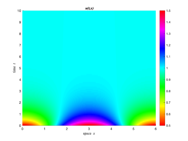
Numerical Experiment 1. In this numerical experiment, we explore the global stability of the constant solution . First, we let and initial function . We observe that as time goes by, the numerical solution of converges to (see Figure 2 (a) for the limit of and (b) for the evolution of ). Note that solves
| (6.1) |
Hence, if converges to some function as , then converges to as , where is the unique solution of (6.1) with being replaced by . In Figure 2 as well as all other figures, except Figure 6, we then only present the limit profile and evolution of as changes. The same phenomenon can be seen when is replaced by . In fact, we have and then for any and . Hence we do not present the pictures for this initial function.


Next, we take , which is very close to . The same phenomenon is observed as well (see Figure 3). To see numerically whether the positive constant solution is globally stable, we also choose initial functions . All the other parameters remain the same. We observe that the numerical solution eventually converges to for each initial function.


Observations from Experiment 1. It is known that the constant solution is locally stable when , is unstable when , and super-critical pitchfork bifurcations occurs when passes through . It is observed from the experiment 1 that the constant solution is also stable with respect to large perturbations when . We conjecture that the constant solution is globally stable when .
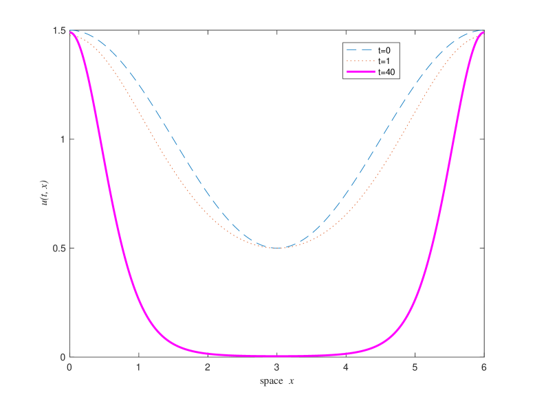
Numerical Experiment 2. In this numerical experiment, we explore the global bifurcation of the constant solution . First of all, we choose , which is slightly larger than the first bifurcation value. Let . We observe that the numerical solution of changes very little when large enough and converges to a nonconstant stationary solution , which is close to the constant solution and corresponds to the analytical nonconstant stationary solution described in the first formula of (3.5) (see Figure 4 for the profile of the numerical solution at , which is close to the profile of the nonconstant stationary solution). This implies that, when , there exist two nonconstant stationary solutions and , where , , a fact that can be seen from the formulas (3.5) and (3.6).


Next, we increase the value of . Let , which is not close to the bifurcation value . Let . All the other parameters remain the same. We observe that as time evolves, the numerical solution of converges to a nonconstant stationary solution, the -component of which has a spike near the boundary (see Figure 5), but the -component does not develop spikes (see Figure 6).


We further increase the value of . Let and take . The same phenomenon is observed (see Figure 7). In particular, we observe that when becomes larger, the -component of the numerical nonconstant stationary solution concentrates more towards the boundary (see Figure 7), which is consistent with Theorem 5.1 (3). By symmetry, the solution of (1.1) with initial function converges to a nonconstant stationary solution, which has a spike near the boundary (see Figure 8).


Observations from Experiment 2. For each in the experiment 2, the same phenomenon is observed for the numerical solution with the initial function , that is, the numerical solutions with initial functions and converge to the same nonconstant stationary solution. This indicates the nonconstant stationary solution is stable. According to the theoretical results, super-critical pitchfork bifurcation occurs when passes through and the bifurcation solution is then locally stable for near . Our numerical simulation confirms this result. The numerical simulation also indicates that this local bifurcation branch extends to and the bifurcation solutions are locally stable. Moreover, as increases, the -component of the bifurcation solution develops a spike near the boundary or , but the -component does not develop any spikes. In fact, it is proved in Theorem 4.2 that for any stationary solutions of (1.1), and stay bounded as increases, which implies that the -component of the bifurcation solution does not develop spikes.
6.3 Numerical simulations for the case and
In this subsection, we discuss the numerical simulations for the case and . In this case, it is known that ; is locally asymptotically stable when ; and when passes through , sub-critical pitchfork bifurcation occurs. Throughout this subsection, and .
Numerical Experiment 3. In this numerical experiment, we investigate the global stability of the constant solution . First of all, let and initial function . We observe that as time goes by, the numerical solution of converges to (see Figures 9 and 10).


Next, let , which is slightly smaller than . Let . We observe that the numerical solution of changes very little when time is large enough and converges to the constant stationary solution (see Figures 11 and 12).


For , let . We observe that the numerical solution of , changes very little when time is large enough and converges to nonconstant stationary solutions, which are not so close to the constant stationary solution (see Figures 13 and 14).


Observations from Experiment 3. It is known that when , the constant solution is locally stable; when , is unstable, and sub-critical pitchfork bifurcation occurs when passes through , that is, there are two unstable nonconstant stationary solutions bifurcating from for and is near . It is observed from the experiment 3 that when and is near , the constant stationary solution is not globally stable and there are other locally stable nonconstant stationary solutions, which are on the extension of the local pitchfork bifurcation branch (see more in the observation of experiment 4 in the following).
Numerical Experiment 4. In this experiment, we investigate the global bifurcation of the constant solution . First, let which is slightly larger than the first bifurcation value. Let . As in the case that , we observe that the numerical solution of , changes very little when time is large enough and converge to nonconstant stationary solutions, which are not so close to the constant stationary solution (see Figures 15 and 16).

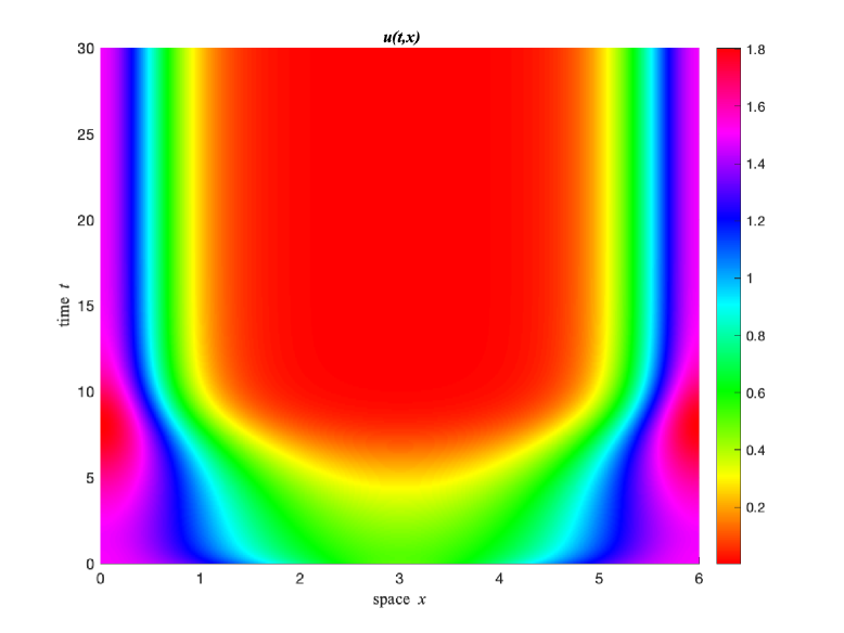


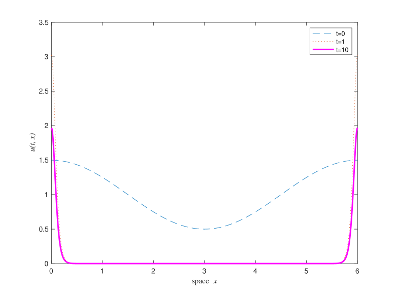
Next, we increase the value of . Let , which is not close to the bifurcation value . Let . All the other parameters remain the same. We observe that as time evolves, the numerical solution of converges to a double boundary spike solution (see Figure 17). The profile of the numerical solution at time can be viewed as the profile of the numerical double boundary spike solution. Let . We observe that the numerical solution of converges to a single interior spike solution (see Figure 18).


We further increase the value of . Let and take . The same phenomenon as in the case is observed (see Figures 19 and 20). In particular, we observe that when becomes larger, the numerical nonconstant stationary solution concentrates more towards both boundaries when and towards the middle of the location when .


Observation from experiment 4. As it is mentioned in the observation of experiment 3, sub-critical pitchfork bifurcation occurs when passes through , that is, there are two unstable nonconstant stationary solutions bifurcating from for and is near . It is observed from the experiment 4 that the local pitchfork bifurcation branch extends to and the bifurcation solutions on the extended branch are locally stable when . Moreover, when increases, the -component of the bifurcation solutions either develops spikes near both boundary points and , or develops an interior spike.
6.4 Numerical simulations for the case , , ,
In this subsection, we discuss the numerical simulations we carried out for the case that , , , and . In this case, it is known that ; is locally asymptotically stable when ; and when passes through , subcritical pitchfork bifurcation occurs. When , similar dynamical scenarios as in the case and are observed numerically. To be more precise, it is observed numerically that when and is near , the constant stationary solution is not globally stable and there are other locally stable nonconstant stationary solutions, which are on the extension of the local pitchfork bifurcation branch. Moreover, in this case, it is observed numerically that, when increases, the -component of the bifurcation solution develops both boundary and interior spikes.
For example, let which is slightly larger than the bifurcation value . Let . We observe that for each initial function, the numerical solution of , changes very little when time is large enough and converges to nonconstant stationary solution, which is not so close to the constant stationary solution (see Figure 21).


Let , which is not close to the bifurcation value . Let . All the other parameters remain the same. We observe that as time evolves, the numerical solution of converges to a spike solution which has boundary spike at and interior spike at (see Figure 22).


Let and take . The same phenomenon as in the case is observed (see Figure 23). In particular, we observe that when becomes larger, the numerical nonconstant stationary solution concentrates more towards the boundary at and the interior at .


References
- [1] H. Amann, Existence and regularity for semilinear parabolic evolution equations, Ann. Scuola Norm. Sup. Pisa Cl. Sci. 11 (1984), no. 4, 593-676.
- [2] X. Bai and M. Winkler, Equilibration in a fully parabolic two-species chemotaxis system with competitive kinetics, Indiana Univ. Math. J. 65 (2016), no. 2, 553–583.
- [3] P. Biler, Global solutions to some parabolic-elliptic systems of chemotaxis, Adv. Math. Sci. Appl., 9 (1999), 347-359.
- [4] C. Cai, Q. Xu, and X. Liu, The local bifurcation and stability of nontrivial steady states of a logistic type of chemotaxis, Acta Math. Appl. Sin. Engl. Ser. 33 (2017), no. 3, 799-808.
- [5] J. Cao, W. Wang, and H. Yu, Asymptotic behavior of solutions to two-dimensional chemotaxis system with logistic source and singular sensitivity, J. Math. Anal. Appl. 436 (2016), no. 1, 382-392.
- [6] J. A. Carrillo, J. Li, and Z. Wang, Boundary spike-layer solutions of the singular Keller-Segel system: existence and stability, Proc. Lond. Math. Soc. (3) 122 (2021), no. 1, 42-68.
- [7] M. G. Crandall, and P. H. Rabinowitz, Bifurcation from simple eigenvalues, J. Funct. Anal. 8, (1971), 321–340.
- [8] W. Du, Asymptotic Behavior of Solutions to a Logistic Chemotaxis System with Singular Sensitivity, Journal of Mathematical Research with Applications , (2021), Vol. 41, No. 5, 473-480.
- [9] K. Fujie and T. Senba, Global existence and boundedness in a parabolic-elliptic Keller-Segel system with general sensitivity, Discrete Contin. Dyn. Syst. Ser. B, 21(1) (2016), 81-102.
- [10] K. Fujie, M. Winkler, and T. Yokota, Blow-up prevention by logistic sources in a parabolic-elliptic Keller-Segel system with singular sensitivity, Nonlinear Anal. 109 (2014), 56-71.
- [11] K. Fujie, M. Winkler, and T. Yokota. Boundedness of solutions to parabolic-elliptic Keller-Segel systems with signal dependent sensitivity, Math. Methods Appl. Sci., 38(6) (2015), 1212-1224.
- [12] D. Henry, Geometric Theory of Semilinear Parabolic Equations, Springer, Berlin, Heidelberg, New York, 1977.
- [13] Q. Wang, L. Zhang, J. Yang, and J. Hu, Global existence and steady states of a two competing species Keller-Segel chemotaxis model, Kinet. Relat. Mod. 8 (2015), 777-807.
- [14] L. Jin, Q. Wang, and Z. Zhang. Pattern formation in Keller–Segel chemotaxis models with logistic growth, Int. J. Bifurcat. Chaos, 26 (2016): 1650033.
- [15] K. Kang, T. Kolokolnikov, and M.J. Ward, The stability and dynamics of a spike in the 1D Keller-Segel model, IMA J. Appl. Math. 72 (2007), no. 2, 140-162.
- [16] E.F. Keller and L.A. Segel, Initiation of slime mold aggregation viewed as an instability, J. Theoret. Biol. 26 (1970) 399-415.
- [17] E.F. Keller and L.A. Segel, Model for chemotaxis, J. Theoret. Biol., 30 (1971), 225-234.
- [18] T. Kolokolnikov, J. Wei, and A. Alcolado, Basic mechanisms driving complex spike dynamics in a chemotaxis model with logistic growth, SIAM J. Appl. Math. 74 (2014), no. 5, 1375-1396.
- [19] F. Kong and Q. Wang, Stability, free energy and dynamics of multi-spikes in the minimal Keller-Segel model, Discrete Contin. Dyn. Syst. 42 (2022), no. 5, 2499-2523.
- [20] F. Kong, J. Wei, and L. Xu, The existence and stability of spikes in the one-dimensional Keller–Segel model with logistic growth, J. Math. Biol. 86 (2023), no. 1, Paper No. 6, 54 pp.
- [21] F. Kong, J. Wei, and L. Xu, Existence of multi-spikes in the Keller–Segel model with logistic growth, Mathematical Models and Methods in Applied Sciences, 33 (2023), 2227-2270.
- [22] H. I. Kurt and W. Shen, Finite-time blow-up prevention by logistic source in parabolic-elliptic chemotaxis models with singular sensitivity in any dimensional setting, https://arxiv.org/abs/2008.01887 ([v4]).
- [23] H. I. Kurt and W. Shen, Chemotaxis models with singular sensitivity and logistic source: Boundedness, persistence, absorbing set, and entire solutions, Nonlinear Analysis: Real World Applications, 69, (2023), 1468-1218.
- [24] H. Li, Spiky steady states of a chemotaxis system with singular sensitivity, J. Dynam. Differential Equations, 30 (2018), no. 4, 1775-1795.
- [25] K. Painter and T. Hillen, Spatio-temporal chaos in a chemotaxis model. Physica D., 240 (2011), 363–375.
- [26] R. Salako, W. Shen, and S. Xue, Can chemotaxis speed up or slow down the spatial spreading in parabolic-elliptic Keller-Segel systems with logistic source? J. Math. Biol. 79 (2019), no. 4, 1455-1490.
- [27] J. Shi and X. Wang, On global bifurcation for quasilinear elliptic systems on bounded domains, J. Differential Equations, 246 (2009), no. 7, 2788-2812.
- [28] Y. Tao and M. Winkler, Large time behavior in a multidimensional chemotaxis-haptotaxis model with slow signal diffusion, SIAM J. Math. Anal. 47 (2015), 4229–4250.
- [29] J.I. Tello and M. Winkler, A chemotaxis system with logistic source, Common Partial Diff. Eq., 32 (2007), 849-877.
- [30] Q. Wang, Y. Song, and L. Shao, Nonconstant positive steady states and pattern formation of 1D prey-taxis systems, J. Nonlinear Sci. 27 (2017), 71-97.
- [31] Q. Wang, J. Yan, and C. Gai, Qualitative analysis of stationary Keller–Segel chemotaxis models with logistic growth, Z. Angew Math. Phys. 67 (2016), no. 3, Art. 51, 25 pp.
- [32] X. Wang and Q. Xu, Spiky and transition layer steady states of chemotaxis systems via global bifurcation and Helly’s compactness theorem, J. Math. Biol., 66 (2013), 1241-1266.
- [33] M. Winkler, Aggregation vs. global diffusive behavior in the higher-dimensional Keller-Segel model, J.Differential Equations., 248 (2010), 2889-2905.
- [34] X. Xu, Existence of spiky steady state of chemotaxis models with logarithm sensitivity, Math. Methods Appl. Sci. 44 (2021), no. 2, 1484-1499.
- [35] X. Zhao. Boundedness to a logistic chemotaxis system with singular sensitivity. arXiv: 2003.03016 v1.