Stability and regularization for ill-posed Cauchy problem of a stochastic parabolic differential equation
Fangfang Dou
Corrsponding author. Email: [email protected].
School of Mathematical Sciences, University of Electronic Science and Technology of China, Chengdu, ChinaPeimin Lü
School of Mathematical Sciences, University of Electronic Science and Technology of China, Chengdu, ChinaYu Wang
School of Mathematics, Southwest Jiaotong University, Chengdu, China.
Abstract
In this paper, we investigate an ill-posed Cauchy problem involving a stochastic parabolic equation. We first establish a Carleman estimate for this equation. Leveraging this estimate, we derive the conditional stability and convergence rate of the Tikhonov regularization method for the aforementioned ill-posed Cauchy problem. To complement our theoretical analysis, we employ kernel-based learning theory to implement the completed Tikhonov regularization method for several numerical examples.
Key Words. Carleman estimate,
Cauchy problem of stochastic parabolic differential equation, conditional stability, regularization, numerical approximation.
1Introduction
To beginning with, we introduce some notations concerning stochastic analysis. More details for these can be found in [24].
Let with be
a complete filtered probability space
on which a one-dimensional standard
Brownian motion is
defined. Let be a Fréchet space. We
denote by the Fréchet
space consisting of all -valued
-adapted processes
such that
;
by the Fréchet space
consisting of all -valued
-adapted bounded
processes; and by
the Fréchet
space consisting of all -valued
-adapted continuous
processes such that
. All of the above spaces
are equipped with the canonical quasi-norms. Furthermore, all of the above spaces
are Banach spaces equipped with the canonical norms, if is a Banach space.
For simplicity, we use the notation where
is the -th coordinate of a generic
point in . In a
similar manner, we use the notation ,
, etc. for the partial derivatives of
and with respect to . Also, we denote
the scalar product in by
, and use to denote a
generic positive constant independent of the
solution , which may change from line to
line.
Let , () be
a given bounded domain with the boundary
, and be a given nonempty open
subset of .
Let
, and .
We assume , , , and
() satisfies
(H1) and
;
(H2)
for some .
Now, the Cauchy problem of the forward stochastic parabolic differential equation can be described as follows.
(1.1)
Let and
The aim of this paper is to study
the Cauchy Problem with the Lateral Data for
the stochastic parabolic differential equation:
Problem (CP) Find
a function
that satisfies system (1.1).
Remark 1.1.
It would be quite interesting to study the general case where .
However, this will lead to the term in (2.28), which we have no idea how to handle.
In certain applications involving diffusive, thermal, and heat transfer problems, measuring some boundary data can be challenging. For instance, in nuclear reactors and steel furnaces in the steel industry, the interior boundary can be difficult to measure. Similarly, the use of liquid crystal thermography in visualization can pose the same problem. To address this issue, engineers attempt to reconstruct the status of the boundary using measurements from the accessible boundary. This, in turn, creates the Cauchy problem for parabolic equations. Due to the requirements in real applications, numerous researchers have focused on solving the Cauchy problem of parabolic differential equations, particularly on the inverse problems for deterministic parabolic equations, as seen in [14, 19, 17, 16, 15, 22, 31, 33], and their respective references. Among these works, some have studied the identification of coefficients in parabolic equations through lateral Cauchy observations, such as uniqueness and stability [14, 33, 19, 31], and numerical reconstruction [15], assuming that the initial value is known. Meanwhile, the determination of the initial value has been considered in [17, 16, 22] under the assumption that all coefficients in the governing equation are known.
Stochastic parabolic equations have a wide range of applications for simulating various behaviors of stochastic models which are utilized in numerous fields such as random growth of bacteria populations, propagation of electric potential in neuron models, and physical systems that are subject to thermal fluctuations (e.g.,[18, 24]). In addition, they can be considered as simplified models for complex phenomena such as turbulence, intermittence, and large-scale structure (e.g.,[8]). Given the significant applications of these models, stochastic parabolic equations have been extensively studied in both physics and mathematics. Therefore, it is natural to study the Cauchy problem of stochastic parabolic equations in such situations. However, due to the complexity of stochastic parabolic equations, some tools become ineffective for solving these problems. Thus, the research on inverse problems for stochastic parabolic differential equations is relatively scarce. In [1], the author proved backward uniqueness of solutions to stochastic semilinear parabolic equations and tamed Navier-Stokes equations driven by linearly multiplicative Gaussian noises, via the logarithmic convexity property known to hold for solutions to linear evolution equations in Hilbert spaces with self-adjoint principal parts. In [11, 27], authors studied inverse random source problems for the stochastic time fractional diffusion equation driven by a spatial Gaussian random field, proving the uniqueness and representation for the inverse problems, as well as proposing a numerical method using Fourier methods and Tikhonov regularization. Carleman estimates play an important role in the study of inverse problems for stochastic parabolic differential equations, such as inverse source problems [23, 35], determination of the history for stochastic diffusion processes [4, 23, 30, 34], and unique continuation properties [6, 32]. We refer the reader to [25] for a survey on some recent advances in Carleman estimates and their applications to inverse problems for stochastic partial differential equations.
In this paper, our objective is to solve Problem (CP), i.e., we aim to retrieve the solution of equation (1.1) with observed data from the lateral boundary. To this end, we first prove the conditional stability based on a new Carleman estimate for the stochastic parabolic equation (1.1). Then we construct a Tikhonov functional for the Cauchy problem based on the Tikhonov regularization strategy and prove the uniqueness of the minimizer of the Tikhonov functional, as well as the convergence rate for the optimization problem using variational principles, Riesz theorems, and Carleman estimates established previously.
Generally, the optimization problem for the Tikhonov functional is difficult to solve in the study of inverse problems in stochastic partial differential equations (SPDEs). This is because it involves solving the adjoint problem of the original problem, which is challenging to handle. In fact, one of the primary differences between stochastic parabolic equations and deterministic parabolic equations is that at least one partial derivative of the solution does not exist, making it impossible to express the solution of that equation explicitly. Fortunately, we can express the mild solution of the stochastic parabolic equations using the fundamental solution of the corresponding deterministic equation[7, 9]. This idea suggests that we can use kernel-based theory to numerically solve the minimization problem of the Tikhonov functional without computing the adjoint problem. Furthermore, we can solve the problem in one step without iteration, thus reducing the computational cost to some extent. This technique has gained attention in the study of numerical computation for ordinary and partial differential equations, and the use of fundamental solutions as kernels has proven effective for solving inverse problems in deterministic evolution partial differential equations. As far as we know, our work is the first attempt to apply the regularization method combining with kernel-based theory to solve inverse problems for stochastic parabolic differential equations.
The strong solution of equation (1.1) is useful in the proof of convergence rate of regularization method. Thus, we recall it here.
Definition 1.1.
We call a solution to the
equation (1.1) if for any and a.e. , it holds
(1.2)
It should be noted that the assumption regarding the solution, namely that , implies a higher degree of smoothness than is strictly necessary for establishing Hölder stability of the Cauchy problem. However, this additional smoothness is required in order to facilitate the regularization process.
The remainder of this paper is organized as follows. Section 2 presents a proof of a Hölder-type conditional stability result, along with the establishment of the Carleman estimate as a particularly useful tool in this proof. The regularization method, using the Tikhonov regularization strategy, is introduced in Section 3 and we showcase both the uniqueness and convergence rate of the regularization solution. Section 4 provides numerically simulated reconstructions aided by kernel-based learning theory.
2Conditional Stability
In this section, we prove a stability estimate for the Cauchy problem.
Theorem 2.1.
(Hölder stability
estimate).
For any given and
, there exists , and a constant
such
that if for ,
(2.1)
then
(2.2)
We first recall the following exponentially
weighted energy identity, which will play a key
role in the sequel.
and . Assume is an
-valued continuous
semi-martingale. Set
and . Then for a.e. and -a.s.
,
(2.4)
where
(2.5)
In the sequel, for a positive integer , denote by a function of order
for large (which is independent
of ); by a function of
order for fixed and for large
.
Proof of Theorem 2.1. We borrow
some idea from [21].
Take a bounded domain such that
and that enjoys a
boundary . Then we have
(2.6)
Let be an
open subdomain. We know that there is a satisfying (see [29, Lemma
5.1] for example)
(2.7)
Since , we can choose a
sufficiently large such that
(2.8)
Further, let
, there exists a positive number such that
(2.9)
Then, define
(2.10)
for a fix , and denote
. Set
(2.11)
Clearly, is independent of . Moreover, for any ,
and thus
Hence, we see in , and thus . On the other
hand, for any ,
Now, we fix in , and
. Let . From (2.36)–(2.38),
we obtain that
which implies that for all , it
holds that
(2.39)
By taking ,
such that
and ,
we get
(2.40)
We now balance the terms in the right hand side of (2) via choosing such
that . This implies that
Hence, for , where the number is so small
that
, we have (2.2) with .
Remark 2.1.
The inequality (2.34) is called the Carleman estimate for (1.1).
3Regularization Method
For , set
Let
Denote . Clearly, we have
(3.1)
Given a function , the
Tikhonov functional is now constructed as
(3.2)
where and .
We have the following result.
Theorem 3.1.
For every ,
there exists a unique minimizer of the functional in (3.2).
Proof. Let
Fix .
We define the inner products as follows:
(3.3)
where .
Let be the completion of with respect to the inner product , and still denoted by for the sake of simplicity.
For , let . Then .
By (3.2), we
should minimize the following
functional
(3.4)
If is a minimizer of the functional
(3.4), then
is a
minimizer of the functional (3.2). On the other hand, if is a minimizer of the functional (3.2),
then is a
minimizer of the functional (3.4).
By the variational principle, any minimizer of the functional (3.4) should satisfy the following condition
In the proof of Theorem 3.1, we utilized solely the variational principle and Riesz’s theorem, without invoking the Carleman estimate. However, we make use of this estimate in Theorem 3.2, where we establish the rate of convergence of minimizers to the precise solution, provided that certain conditions are met.
Assume that there exists an exact solution of the problem (1.1) with the exact data
By
Theorem 2.1, the exact solution is
unique. Because of the existence of there also exists an exact function such that
(3.8)
Here is
an example of such a function . Let
the
function be such that in a small neighborhood
where
is a sufficiently small number. Then
can be constructed as . Let be a sufficiently small number
characterizing the error in the data. We assume
that
(3.9)
and
(3.10)
Theorem 3.2.
(Convergence rate).
Assume (3.9) and (3.10), and let the regularization parameter
, where is a constant. Let , and be the
same as in Theorem 2.1. Then there exists a
sufficiently small number and a constant such that if , then
Since numbers and since , then . Thus, using (3.8),
(3.18) and (3.19), we obtain
(3.11).
4Numerical Approximations
In this section, we aim to numerically solve the ill-posed Cauchy problem of the stochastic parabolic differential equation given by (1.1). For the sake of simplicity, we set , , , and in the system for all numerical tests to follow. Since an explicit expression for the exact solution is unavailable, we resort to numerically solving the initial-boundary value problem
(4.1)
by employing the finite difference method with time discretized via the Euler-Maruyama method [10] to obtain the Cauchy data on . We then construct numerical approximations for the Cauchy problem (1.1) via Tikhonov regularization, with the aid of kernel-based learning theory, for which we have established a convergence rate guaranteed in Section 3.
We verify the proposed method by using following three examples.
Example 4.1.
Let and . Suppose that
(a)
(b)
The simplest time-discrete approximation is the stochastic version of the Euler approximation, also known as the Euler-Maruyama method [10].
We simply describe the process of solving the initial-boundary value problem (4.1) in Example 4.1 by the Euler-Maruyama method in the following.
Let with , , , , where and denote the spatial and temporal step sizes, respectively. It was shown that not all heuristic time-discrete approximations of stochastic differential equations converge to the solution process in a useful sense as the time step size tends to zero [10]. Since the numerical approximation of observations obtained by direct application of backward finite difference scheme is not adapted to the filtration , we can only solve the initial-boundary value problem (4.1) by the explicit finite difference scheme, i.e.,
where the initial and boundary value are given by
To ensure the numerical scheme is stable, we choose and in the computation.
By solving above algebraic system, we obtain distribution of at meshed grids of the initial-boundary value problem (4.1). In the process of solving Cauchy problem (1.1) numerically, we using and instead of the Cauchy data at .
In the following, we numerically solve the optimization problem which is given in (3.2) by kernel-based learning theory.
Suppose that is the fundamental solution of parabolic equation
then the mild solution of
(4.2)
can be written as
(4.3)
Since the fundamental solution is deterministic, so the mild solution given by (4.3) is well-known.
Assume that
(4.4)
Here are the basis functions, is the number of source points, and are unknown coefficients to be determined.
From (4.3), we can let , where is the fundamental solution of the deterministic parabolic equation, are source points.
The suitable choice of the source points can ensure that is analytic in the domain and make the algorithm effective and accurate.
However, the optimal rule for the location of source points is still open. In recent work, we occupy uniformly distributed points on below , where and are post-prior determined, as the source points. This choice is given in [5] and related works, and performs better in comparison with other schemes.
Since be given in (4.4) has already satisfied the equation in system (4.1), coefficients should be determined by Cauchy conditions.
From the process of solving the initial boundary value problem we know that, and can be set as the collocation points, and the problem converts to solving unknowns
from the linear system
(4.5)
where
and
By comparing the Tikhonov functional be given in (3.2) we know, is calculated by .
Choosing the regularization parameter by using the L-curve method, that is, a regularized solution near the “corner” of the L-curve [12]
and denoting the regularized solution of linear system (4.5) by , leads to the approximated solution
To illustrate the comparison of the exact solution and its approximation and in order to avoid “inverse crime”, we choose and compute by finite difference method again such that and be defined on the same grid.
Figure 4.1 shows the numerical solution of the initial-boundary problem and the approximation solutions of the Cauchy problem of Example 4.1(a) with different noisy levels. Since the data is given at , the numerical solution seems worse as tends to , this is consistence with the convergence estimation in section 3 because no information is given at partial boundary . Furthermore, the convergence rate always holds in the temporal interval in section 3. However, from this figure, we find that the proposed method also works well at .
Denote the relative error by
(4.7)
(a)
(b)
(c)
Figure 4.1: Approximated solution with different noisy levels of Example 4.1(a).
As in the study of stochastic equations, large numbers of sample paths should be checked in the numerical experiments for simulating the expectation of the solution. Thus, we do the tests with different sample paths. It is interesting from Figure 4.2 that when the number of sample paths is great than 10, the results seems no better off. Thus in the following, we only consider do the experiments with number of sample paths
(a)Relative errors
(b)Numerical approximations of
Figure 4.2: Numerical results by expectation of solutions of different numbers of sample paths.
Now we consider the problem in Example 4.1(b). In this case, is a piecewise smooth function.
Figure 4.3 shows the approximations of boundary value in (a) and the approximations of initial value with different noise levels in (b). Moreover, to illustrate the effectiveness of the proposed method, the change of relative error along lines and are also given in Figure 4.3(c) and (d), respectively.
(a)Approximations of
(b)Approximations of
(c)Relative errors
(d)Relative errors
Figure 4.3: Numerical results of Example 4.1(b) with different noisy level data .
We mention that the Cauchy problem of the deterministic parabolic equation has been considered in [20], that the numerical algorithm based on Carleman weight function proposed can stably invert the solution near the known boundary conditions, more precisely, solutions for for 1-D example. With comparison of the results of Example 4.1, our method works well for recovering the solution for for the stochastic parabolic equation. We believe this algorithm also works well for deterministic parabolic equation, and can be an improvement of previous works. Furthermore, the proposed method also works well for 2-D examples in both rectangular and discal domains.
We explore the effectiveness of the proposed numerical methods in following two examples in bounded domains in , as well as the influence of parameter in the kernel-based learning method. We always let unless particularly stated.
Example 4.2.
Suppose that , and . Let
(a)
(b)
We first consider the optimal choices of parameters and in case that the Cauchy data are given on in the kernel-based approximation processes. We set and observe relative errors with the change of . It can be seen from figure 4.4 that , the methods performs well. Numerical results in Figure 4.5 illustrate that any is a reasonable choice. Thus we fix in the following computing.
The numerical approximations and relative errors for different noise level are shown in Figure 4.6.
Figure 4.4: The relative error for different .Figure 4.5: The relative error for different .
(a)approximation with
(b)approximation with
(c)approximation with
(d)relative error with
(e)relative error with
(f)relative error with
Figure 4.6: The approximations for and relative errors for different noise levels for Example 4.2(a).
According to the conditional stability and convergence estimate we analyzed in section 2 and 3, the length of partial of boundary for which Cauchy data be given, will also effect on the approximation. Thus, we verify the proposed method for this example with Cauchy data be given in by Figure 4.7.
(a)approximation with data on
(b)approximation with data on
(c)approximation with data on
(d)relative error with data on
(e)relative error with data on
(f)relative error with data on
Figure 4.7: Approximations and relative errors for Example 4.2(b) with Cauchy data be given on different partial of boundary.
In Example 4.2, is a rectangular domain that the initial-boundary problem could be computed well by the finite difference method. However, in case that is a general bounded domain, we should improve the finite difference method by heterogeneous grids. To avoid the complicated analysis for the numerical solution of initial-boundary problem, we solve the problem by kernel-based learning theory, by treating the fundamental solution as kernels.
Example 4.3.
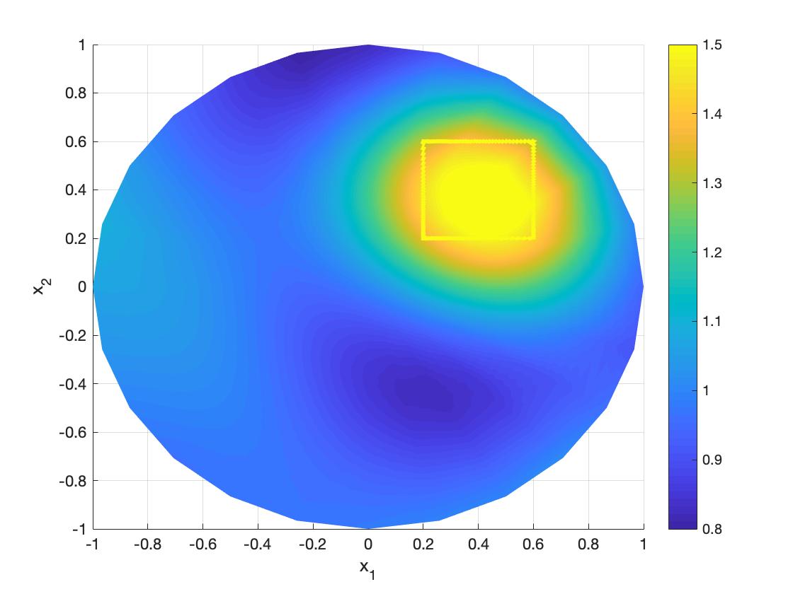
Suppose that , where , , and . Let
We show the numerical results when with varies and results with different partial of boundary for for in Figure 4.8 and 4.9, respectively.
(a)approximation with
(b)approximation with
(c)approximation with
(d)relative error with
(e)relative error with
(f)relative error with
Figure 4.8: Numerical results with different noisy level for Example 4.3.
(a)approximation with data on
(b)approximation with data on
(c)approximation with data on
(d)relative error with data on
(e)relative error with data on
(f)relative error with data on
Figure 4.9: Numerical results with Cauchy data on different partial boundary for Example 4.3.
In conclusion, we do the numerical experiments for the Cauchy problem of stochastic parabolic equation for examples on both 1-D and 2-D bounded domains by smooth, piecewise smooth and noncontinuous initial conditions, numerical results illustrate that the proposed method works well for all these examples. Although we haven’t solved examples for other irregular 2-D domains and 3-D domains, it can be seen from the kernel-based learning theory that the method should be satisfied, because there is no limitation of dimension and shape of domains in the kernel-based learning theory but only distances between source points and collection point be concerned. Moreover, since no iterated method used in the numerical computation, the computational cost is reduced. However, the convergence rate for the kernel-based learning theory is still open.
Acknowledgement
The authors would like to thank Professor Kui Ren for providing valuable suggestions. This work is partially supported by the NSFC (No. 12071061), the Science Fund for Distinguished Young Scholars of Sichuan Province (No. 2022JDJQ0035).
References
[1]
V. Barbu and M. Röckner.
Backward uniqueness of stochastic parabolic like equations driven by
gaussian multiplicative noise.
Stochastic Processes and their Applications, 126(7):2163–2179,
2016.
[2]
L. Beilina and M.V. Klibanov.
Approximate global convergence and adaptivity for coefficient
inverse problems.
Springer Science & Business Media, 2012.
[3]
R.C. Dalang, D. Khoshnevisan, C. Müller, D. Nualart, and Y.M.
Xiao.
A minicourse on stochastic partial differential equations,
volume 1962.
Springer, 2009.
[4]
F.F. Dou and W. Du.
Determination of the solution of a stochastic parabolic equation by
the terminal value.
Inverse Problems, 38(7):075010, 2022.
[5]
F.F. Dou and Y.C. Hon.
Kernel-based approximation for cauchy problem of the time-fractional
diffusion equation.
Engineering Analysis with Boundary Elements, 36(9):1344–1352,
2012.
[6]
X. Fu and X. Liu.
A weighted identity for stochastic partial differential operators and
its applications.
Journal of Differential Equations, 262(6):3551–3582, 2017.
[7]
J.B. Walsh.
An introduction to stochastic partial differential equations.
Springer, 1986.
[8] J. Glimm.
Nonlinear and stochastic phenomena:
the grand challenge for partial differential
equations.SIAM Review, 33, 626–643, 1991.
[9]T. Takeshi.
Successive approximations to solutions of stochastic differential equations.Journal of Differential Equations, 96, 152-199, 1992.
[10]
P.E. Kloeden,and E. Platen.
Numerical Solution of Stochastic Differential Equations.Springer, 1992.
[11]
Y. Gong, P. Li, X. Wang, and X. Xu.
Numerical solution of an inverse random source problem for the time
fractional diffusion equation via phaselift.
Inverse Problems, 37(4):045001, 2021.
[12]
P.C. Hansen.
Numerical tools for analysis and solution of fredholm integral
equations of the first kind.
Inverse Problems, 8(6):849-872, 1992.
[13]
Y.C. Hon and T. Wei.
A fundamental solution method for inverse heat conduction problem.
Engineering Analysis with Boundary Elements, 28(5):489–495,
2004.
[14]
V. Isakov and S. Kindermann.
Identification of the diffusion coefficient in a one-dimensional
parabolic equation.
Inverse Problems, 16(3):665–680, 2000.
[15]
Y.L. Keung and J. Zou.
Numerical identifications of parameters in parabolic systems.
Inverse Problems, 14(1):83–100, 1998.
[16]
M.V. Klibanov and A.V. Tikhonravov.
Estimates of initial conditions of parabolic equations and
inequalities in infinite domains via lateral cauchy data.
Journal of Differential Equations, 237(1):198–224, 2007.
[17]
M.V. Klibanov.
Estimates of initial conditions of parabolic equations and
inequalities via lateral Cauchy data.
Inverse Problems, 22(2):495, 2006.
[18] P. Kotelenez. Stochastic ordinary and
stochastic partial differential equations.
Transition from microscopic to macroscopic
equations.
Springer, New York, 2008.
[19]
M.V. Klibanov.
Carleman estimates for global uniqueness, stability and numerical
methods for coefficient inverse problems.
Journal of Inverse and Ill-Posed Problems, 21(4):477–560,
2013.
[20]
Klibanov, Michael V.; Koshev, Nikolaj A.; Li, Jingzhi; Yagola, Anatoly G.
Numerical solution of an ill-posed Cauchy problem for a quasilinear parabolic equation using a Carleman weight function
Journal of Inverse and Ill-Posed Problems, 24(6):761–776, 2016.
[21]
H. Li and Q. Lü.
A quantitative boundary unique continuation for stochastic parabolic
equations.
Journal of Mathematical Analysis and Applications,
402(2):518–526, 2013.
[22]
J. Li, M. Yamamoto, and J. Zou.
Conditional stability and numerical reconstruction of initial
temperature.
Communications on Pure & Applied Analysis, 8(1):361–382,
2009.
[23]
Q. Lü.
Carleman estimate for stochastic parabolic equations and inverse
stochastic parabolic problems.
Inverse Problems, 28(4):045008, 2012.
[24]
Q. Lü and X. Zhang.
Mathematical control theory for stochastic partial differential equations. Springer, Cham, 2021.
[25]
Q. Lü and X. Zhang.
Inverse problems for stochastic partial differential equations: Some
progresses and open problems,
Numerical Algebra, Control and Optimization, 2023, DOI: 10.3934/naco.2023014.
[26]
K.R. Müller, S. Mika, K. Tsuda, G. Ratschnd K. Schölkopf.
An introduction to kernel-based learning algorithms.
In IEEE Transactions on Neural Networks, 12(2):181:201, 2001.
[27]
P. Niu, T. Helin, and Z. Zhang.
An inverse random source problem in a stochastic fractional diffusion
equation.
Inverse Problems, 36(4):045002, 2020.
[28]
R. Schaback.
Convergence of unsymmetric kernel-based meshless collocation methods.
SIAM Journal on Numerical Analysis, 45(1):333–351, 2007.
[29]
S. Tang and X. Zhang.
Null controllability for forward and backward stochastic parabolic
equations.
SIAM Journal on Control and Optimization, 48(4):2191–2216,
2009.
[30]
B. Wu, Q. Chen, and Z. Wang.
Carleman estimates for a stochastic degenerate parabolic equation and
applications to null controllability and an inverse random source problem.
Inverse Problems, 36(7):075014, 2020.
[31]
M. Yamamoto.
Carleman estimates for parabolic equations and applications.
Inverse Problems, 25(12):123013, 2009.
[32]
Z. Yin.
A quantitative internal unique continuation for stochastic parabolic
equations.
Mathematical Control and Related Fields, 5(1):165–176, 2015.
[33]
G. Yuan and M. Yamamoto.
Lipschitz stability in the determination of the principal part of a
parabolic equation.
ESAIM: Control, Optimisation and Calculus of Variations,
15(3):525–554, 2009.
[34]
G. Yuan.
Conditional stability in determination of initial data for stochastic
parabolic equations.
Inverse Problems, 33(3):035014, 2017.
[35]
X. Zhang.
Unique continuation for stochastic parabolic equations.
Differential Integral Equations, 21:81–93, 2008.