This paper was converted on www.awesomepapers.org from LaTeX by an anonymous user.
Want to know more? Visit the Converter page.

Stability and Regularity for Double Wall Carbon Nanotubes Modeled as Timoshenko Beams with Thermoelastic Effects and Intermediate Damping

Fredy M. Sobrado Suárez
Department of Mathematics, The Federal University of Technological of Paraná, Brazil
Lesly D. Barbosa Sobrado, Gabriel L. Lacerda de Araujo 
Institute of Mathematics, Federal University of Rio de Janeiro, Brazil
and  Filomena B. Rodrigues Mendes
Department of Engenhary Electric, The Federal University of Technological of Paraná, Brazil
Abstract

This research studies two systems composed by the Timoshenko beam model for double wall carbon nanotubes, coupled with the heat equation governed by Fourier’s law. For the first system, the coupling is given by the speed the rotation of the vertical filament in the beam βψt\beta\psi_{t} from the first beam of Tymoshenko and the Laplacian of temperature δθxx\delta\theta_{xx}, where we also consider the damping terms fractionals γ1(xx)τ1ϕt\gamma_{1}(-\partial_{xx})^{\tau_{1}}\phi_{t}, γ2(xx)τ2yt\gamma_{2}(-\partial_{xx})^{\tau_{2}}y_{t} and γ3(xx)τ3zt\gamma_{3}(-\partial_{xx})^{\tau_{3}}z_{t}, where (τ1,τ2,τ3)[0,1]3(\tau_{1},\tau_{2},\tau_{3})\in[0,1]^{3}. For this first system we proved that the semigroup S1(t)S_{1}(t) associated to system decays exponentially for all (τ1,τ2,τ3)[0,1]3(\tau_{1},\tau_{2},\tau_{3})\in[0,1]^{3}. The second system also has three fractional damping γ1(xx)β1ϕt\gamma_{1}(-\partial_{xx})^{\beta_{1}}\phi_{t}, γ2(xx)β2yt\gamma_{2}(-\partial_{xx})^{\beta_{2}}y_{t} and γ3(xx)β3zt\gamma_{3}(-\partial_{xx})^{\beta_{3}}z_{t}, with (β1,β2,β3)[0,1]3(\beta_{1},\beta_{2},\beta_{3})\in[0,1]^{3}. Furthermore, the couplings between the heat equation and the Timoshenko beams of the double wall carbon nanotubes for the second system is given by the Laplacian of the rotation speed of the vertical filament in the beam βψxxt\beta\psi_{xxt} of the first beam of Timoshenko and the Lapacian of the temperature δθxx\delta\theta_{xx}. For the second system, we prove the exponential decay of the associated semigroup S2(t)S_{2}(t) for (β1,β2,β3)[0,1]3(\beta_{1},\beta_{2},\beta_{3})\in[0,1]^{3} and also show that this semigroup admits Gevrey classes s>(ϕ+1)/(2ϕ)s>(\phi+1)/(2\phi) for ϕ=min{β1,β2,β3},(β1,β2,β3)(0,1)3\phi=\min\{\beta_{1},\beta_{2},\beta_{3}\},\forall(\beta_{1},\beta_{2},\beta_{3})\in(0,1)^{3}, and we finish our investigation proving that S2(t)S_{2}(t) is analytic when the parameters (β1,β2,β3)[1/2,1]3(\beta_{1},\beta_{2},\beta_{3})\in[1/2,1]^{3}. One of the motivations for this research was the work recently published in 2023; Ramos et al. [20], whose partial results are part of our results obtained for the first system for (τ1,τ2,τ3)=(0,0,0)(\tau_{1},\tau_{2},\tau_{3})=(0,0,0).

corresponding author:e-mail: [email protected] (Fredy M. Sobrado Suárez)

.


keyword: Asymptotic Behavior, Stability, Regularity, Analyticity, DWCNTs-Fourier System, Gevrey Class.

1 Introduction

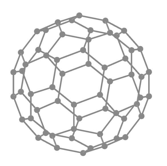
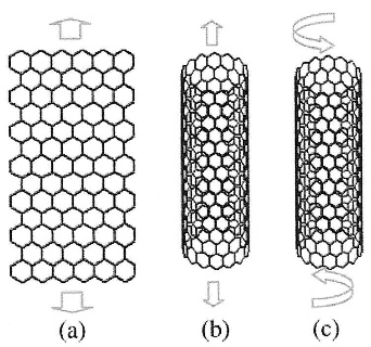
The discovery of structures called carbon nanotubes (CNTs) occurred in 1987 and later officially disclosed to the scientific community in 1991 [11] as the multi wall carbon nanotubes (MWCNTs); they were discovered experimentally in the search for a molecular structure called Fullerene. Fullerene is a closed carbon structure with a spherical format (geodesic dome) formed by 12 pentagons and 20 hexagons, whose formula is C60C_{60}. Carbon nanotubes are cylindrical macromolecules composed of carbon atoms in a periodic hexagonal array with sp2sp^{2} hybridization, similar to graphite [9]. They are made like rolled sheets of graphene and can be as thick as a single carbon atom. They receive this name due to their tubular morphology in nanometric dimensions (1nm=109m.1nm=10^{-9}m.). According to Shen and Brozena [24], CNTs are classified in three ways: single wall carbon nanotubes (SWCNTs), double wall carbon nanotubes (DWCNTs) and (MWCNTs), where the concentric cylinders interact with each other through the Van der Walls force, the authors also point out that DWCNTs are an emerging class of carbon nanostructures and represent the simplest way to study the physical effects of coupling between the walls of carbon nanotubes.

Refer to caption
Figure 1: Fullerene C60C_{60}
Refer to caption
Figure 2: Nanotube structure [25]

The discovery of this new structure at the molecular level contributed in the last decade to the advancement of nanotechnology. In [31] an analysis of the main properties of CNTs was presented, the study confirmed that CNTs have excellent properties; mechanical, electronic and chemical; they are about ten times stronger and six times lighter than steel. They transmit electricity like a superconductor and are excellent transmitters of temperature. Due to their superior electronic and mechanical properties to currently used materials, carbon nanotubes are candidates to be used in products and equipment that require nanoscale structures.

In the future, CNTs should become the base material for nanoelectronics, nanodevices, and nanocomposites. The main problems that have to be overcome for this to happen are the difficult controlled experiments at the nanoscale: the high cost of molecular dynamics simulations and the high time consumption of these simulations. Knowing better the models of continuous mechanics, which are governed by the modeling through the Euler elastic beam model and the Timoshenko beam model used to study the mechanics of linear and nonlinear deformations, should help to make this possible.

The Euler-Bernoulli beam model disregards the effects of shear and rotation, and according to [30, 31] the vibrations in carbon nanotubes are animated by high frequencies, above 1Thz1Thz. According to Yoon and others [34], the effects of rotational inertia and shear are significant in the study of terahertz frequencies (101210^{12}), hence Yoon [34] considers questionable the Euler-Bernoulli model applied to (CNTs). Therefore, the Timoshenko Model is the most suitable. For double-walled nanotubes (DWCNTs) or concentric multi-walled nanotubes (MWCNTs), the most used continuous models in the literature assume that all nested tubes of MWCNTs remain coaxial during deformation and thus can be described by a single deflection model. However, this model cannot be used to describe the relative vibration between adjacent tubes of MWCNTs. In 2003, it was proposed by [31] that the fittings of concentric tubes are considered as individual beams, and that the deflections of all nested tubes are coupled through the van der Waals interaction force between two adjacent tubes [3, 4]. So, each of the inner and outer tubes is modeled as a beam.

In the pioneering work on the carbon nanotube model by Yoon et al. [33], the authors proposed a coupled system of partial differential equations inspired by the Timoshenko beam model to model DWCNTs. The model consists of the following equations

ρA12Y1t2κGA1(2Y1x2φ1x)P\displaystyle\rho A_{1}\dfrac{\partial^{2}Y_{1}}{\partial t^{2}}-\kappa GA_{1}\bigg{(}\dfrac{\partial^{2}Y_{1}}{\partial x^{2}}-\dfrac{\partial\varphi_{1}}{\partial x}\bigg{)}-P =\displaystyle= 0,\displaystyle 0,
ρI12φ1t2EI12φ1x2κGA1(Y1xφ1)\displaystyle\rho I_{1}\dfrac{\partial^{2}\varphi_{1}}{\partial t^{2}}-EI_{1}\dfrac{\partial^{2}\varphi_{1}}{\partial x^{2}}-\kappa GA_{1}\bigg{(}\dfrac{\partial Y_{1}}{\partial x}-\varphi_{1}\bigg{)} =\displaystyle= 0,\displaystyle 0,
ρA22Y2t2κGA2(2Y2x2φ2x)+P\displaystyle\rho A_{2}\dfrac{\partial^{2}Y_{2}}{\partial t^{2}}-\kappa GA_{2}\bigg{(}\dfrac{\partial^{2}Y_{2}}{\partial x^{2}}-\dfrac{\partial\varphi_{2}}{\partial x}\bigg{)}+P =\displaystyle= 0,\displaystyle 0,
ρI22φ2t2EI22φ2x2κGA2(Y2xφ2)\displaystyle\rho I_{2}\dfrac{\partial^{2}\varphi_{2}}{\partial t^{2}}-EI_{2}\dfrac{\partial^{2}\varphi_{2}}{\partial x^{2}}-\kappa GA_{2}\bigg{(}\dfrac{\partial Y_{2}}{\partial x}-\varphi_{2}\bigg{)} =\displaystyle= 0.\displaystyle 0.

Where YiY_{i} and φi\varphi_{i} (i=1,2i=1,2) represent respectively the total deflection and the inclination due to the bending of the nanotube ii and the constants IiI_{i}, AiA_{i} denote the moment of inertia and the cross-sectional area of the tube ii, respectively, and PP is the Van der Waals force acting on the interaction between the two tubes per unit of axial length. Also according to [33], it can be seen that the deflections of the two tubes are coupled through the Van der Waals interaction PP (see [29]) between the two tubes, and as the tubes inside and outside of a DWCNTs are originally concentric, the Van der Waals interaction is determined by the spacing between the layers. Therefore, for a small-amplitude linear vibration, the interaction pressure at any point between the two tubes linearly depends on the difference in their deflection curves at that point, that is, it depends on the term

P=ȷ(Y2Y1).P=\jmath(Y_{2}-Y_{1}). (1)

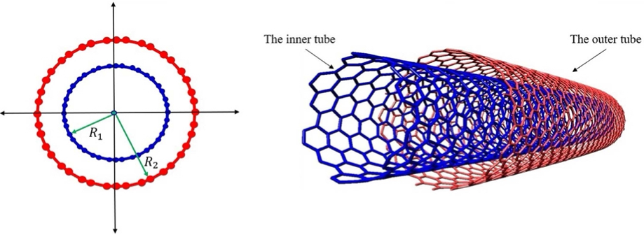
In particular, the Van der Waals interaction coefficient ȷ\jmath for the interaction pressure per unit axial length can be estimated based on an effective interaction width of the tubes as found in [32, 21]. Thus, this model treats each of the nested and concentric nanotubes as individual Timoshenko beams interacting in the presence of Van der Waals forces (see Figure: (3)).

Refer to caption
Figure 3: 2D and 3D Representations of the Double Wall Carbono Nanotubes Model [20]

Currently in the literature there are few investigations related to the study of asymptotic behavior and/or regularity for DWCNTs models, or for DWCNTs systems coupled with the heat equation governed by Fourier’s law (DWCNTs-Fourier). The DWCNTs model was studied in 2015 in the thesis [17], where the author studied the asymptotic behavior of the model:

ρ1φttκ1(φxψ)xȷ(yφ)+α0φt=0in(0,l)×(0,),\displaystyle\rho_{1}\varphi_{tt}-\kappa_{1}(\varphi_{x}-\psi)_{x}-\jmath(y-\varphi)+\alpha_{0}\varphi_{t}=0\quad{\rm in}\quad(0,l)\times(0,\infty), (2)
ρ2ψttb1ψxxκ1(φxψ)+α1ψt=0in(0,l)×(0,),\displaystyle\rho_{2}\psi_{tt}-b_{1}\psi_{xx}-\kappa_{1}(\varphi_{x}-\psi)+\alpha_{1}\psi_{t}=0\quad{\rm in}\quad(0,l)\times(0,\infty), (3)
ρ3yttκ2(yxz)x+ȷ(yφ)+α2yt=0in(0,l)×(0,),\displaystyle\rho_{3}y_{tt}-\kappa_{2}(y_{x}-z)_{x}+\jmath(y-\varphi)+\alpha_{2}y_{t}=0\quad{\rm in}\quad(0,l)\times(0,\infty), (4)
ρ4zttb2zxxκ2(yxz)+α3zt=0in(0,l)×(0,),\displaystyle\rho_{4}z_{tt}-b_{2}z_{xx}-\kappa_{2}(y_{x}-z)+\alpha_{3}z_{t}=0\quad{\rm in}\quad(0,l)\times(0,\infty), (5)

with the initial conditions

φ(x,0)=φ0(x),φt(x,0)=φ1(x),ψ(x,0)=ψ0(x),ψt(x,0)=ϕ1(x)\displaystyle\varphi(x,0)=\varphi_{0}(x),\quad\varphi_{t}(x,0)=\varphi_{1}(x),\quad\psi(x,0)=\psi_{0}(x),\quad\psi_{t}(x,0)=\phi_{1}(x) inx(0,l),\displaystyle{\rm in}\quad x\in(0,l), (6)
y(x,0)=y0(x),yt(x,0)=y1(x),z(x,0)=z0(x),zt(x,0)=z1(x)\displaystyle y(x,0)=y_{0}(x),\quad y_{t}(x,0)=y_{1}(x),\quad z(x,0)=z_{0}(x),\quad z_{t}(x,0)=z_{1}(x) inx(0,l),\displaystyle{\rm in}\quad x\in(0,l), (7)

and subject to boundary conditions

φ(0,t)=φ(l,t)=ψ(0,t)=ψ(l,t)=0forallt>0,\displaystyle\varphi(0,t)=\varphi(l,t)=\psi(0,t)=\psi(l,t)=0\quad{\rm for\quad all}\quad t>0, (8)
y(0,t)=y(l,t)=z(0,t)=z(l,t)=0forallt>0.\displaystyle y(0,t)=y(l,t)=z(0,t)=z(l,t)=0\quad{\rm for\quad all}\quad t>0. (9)

For the case that α0=0\alpha_{0}=0 and αi>0\alpha_{i}>0, for i=1,2,3i=1,2,3, in [17] the author demonstrated the lack of exponential decay of the semigroup (S(t))t0(S(t))_{t\geq 0} associated with the system (2)–(9), when ρ1κ1ρ2b1\frac{\rho_{1}}{\kappa_{1}}\not=\frac{\rho_{2}}{b_{1}} and ȷ(ρ2b1ρ1κ1)κ1b1\jmath\big{(}\frac{\rho_{2}}{b_{1}}-\frac{\rho_{1}}{\kappa_{1}}\big{)}\not=\frac{\kappa_{1}}{b_{1}}, and also proved that if χ=κ1ρ2b1ρ1κ12ȷρ2κ1+ȷb1ρ1=0\chi=\frac{\kappa_{1}\rho_{2}-b_{1}\rho_{1}}{\kappa_{1}^{2}-\jmath\rho_{2}\kappa_{1}+\jmath b_{1}\rho_{1}}=0, then (S(t))t0(S(t))_{t\geq 0} is exponentially stable, and if χ0\chi\not=0, (S(t))t0(S(t))_{t\geq 0} is exponentially stable. Beyond, is proved that if χ0\chi\not=0, then (S(t))t0(S(t))_{t\geq 0} is polynomially stable with optimal rate o(t12)o(t^{-\frac{1}{2}}). In addition, in Chapter 4 of [17], the author validates through numerical analysis, using the finite difference method, the results previously demonstrated, and in addition to presenting graphs of other cases, such as considering αi=0\alpha_{i}=0 and αi>0\alpha_{i}>0 for i=1,2,3,4i=1,2,3,4.

Recently, in 2023, two new investigations emerged: One of them is the DWCNTs-Fourier system with friction dampers, see [20]; in this work the authors consider the problem of heat conduction in carbon nanotubes modeled as Timoshenko beams, inspired by the work of Yoon et al. [Comp. Part B: Ing. 35 (2004) 87–93]. The system is given by

ρ1φttκ1(φxψ)xȷ(yφ)+γ1φt=0in(0,l)×(0,),\displaystyle\rho_{1}\varphi_{tt}-\kappa_{1}(\varphi_{x}-\psi)_{x}-\jmath(y-\varphi)+\gamma_{1}\varphi_{t}=0\quad{\rm in}\quad(0,l)\times(0,\infty), (10)
ρ2ψttb1ψxxκ1(φxψ)+δθxx=0in(0,l)×(0,),\displaystyle\rho_{2}\psi_{tt}-b_{1}\psi_{xx}-\kappa_{1}(\varphi_{x}-\psi)+\delta\theta_{xx}=0\quad{\rm in}\quad(0,l)\times(0,\infty), (11)
ρ3yttκ2(yxz)x+ȷ(yφ)+γ2yt=0in(0,l)×(0,),\displaystyle\rho_{3}y_{tt}-\kappa_{2}(y_{x}-z)_{x}+\jmath(y-\varphi)+\gamma_{2}y_{t}=0\quad{\rm in}\quad(0,l)\times(0,\infty), (12)
ρ4zttb2zxxκ2(yxz)+γ3zt=0in(0,l)×(0,),\displaystyle\rho_{4}z_{tt}-b_{2}z_{xx}-\kappa_{2}(y_{x}-z)+\gamma_{3}z_{t}=0\quad{\rm in}\quad(0,l)\times(0,\infty), (13)
ρ5θtKθxx+βψt=0in(0,l)×(0,),\displaystyle\rho_{5}\theta_{t}-K\theta_{xx}+\beta\psi_{t}=0\quad{\rm in}\quad(0,l)\times(0,\infty), (14)

subject to boundary conditions (8), (9) and

θ(0,t)=θ(l,t)=0 for allt>0.\theta(0,t)=\theta(l,t)=0\qquad\text{ for all}\quad t>0. (15)

Note that the system (8)–(15) presents three friction dissipators (weak damping): γ1φt,γ2yt\gamma_{1}\varphi_{t},\gamma_{2}y_{t} and γ3zt\gamma_{3}z_{t}. The authors apply semigroup theory of linear operators to demonstrate the exponential stabilization of the semigroup S(t)S(t) associated with the system (8)–(15), and their results are independent of the relationship between the coefficients. Furthermore, they analyze the totally discrete problem using a finite difference scheme, introduced by a space-time discretization that combines explicit and implicit integration methods. The authors also show the construction of numerical energy and simulations that validate the theoretical results of exponential decay and convergence rates.

By the year of 2023, [22] investigated the one-dimensional equations for the double wall carbon nanotubes modeled by coupled Timoshenko elastic beam system with nonlinear arbitrary localized damping:

ρ1φttκ1(φxψ)xȷ(yφ)+α1(x)g1(φt)=0in(0,l)×(0,),\displaystyle\rho_{1}\varphi_{tt}-\kappa_{1}(\varphi_{x}-\psi)_{x}-\jmath(y-\varphi)+\alpha_{1}(x)g_{1}(\varphi_{t})=0\quad{\rm in}\quad(0,l)\times(0,\infty), (16)
ρ2ψttb1ψxxκ1(φxψ)+α2(x)g2(ψt)=0in(0,l)×(0,),\displaystyle\rho_{2}\psi_{tt}-b_{1}\psi_{xx}-\kappa_{1}(\varphi_{x}-\psi)+\alpha_{2}(x)g_{2}(\psi_{t})=0\quad{\rm in}\quad(0,l)\times(0,\infty), (17)
ρ3yttκ2(yxz)x+ȷ(yφ)+α3(x)g3(yt)=0in(0,l)×(0,),\displaystyle\rho_{3}y_{tt}-\kappa_{2}(y_{x}-z)_{x}+\jmath(y-\varphi)+\alpha_{3}(x)g_{3}(y_{t})=0\quad{\rm in}\quad(0,l)\times(0,\infty), (18)
ρ4zttb2zxxκ2(yxz)+α4(x)g4(zt)=0in(0,l)×(0,),\displaystyle\rho_{4}z_{tt}-b_{2}z_{xx}-\kappa_{2}(y_{x}-z)+\alpha_{4}(x)g_{4}(z_{t})=0\quad{\rm in}\quad(0,l)\times(0,\infty), (19)

where the localizing functions αi(x)\alpha_{i}(x) are supposed to be smooth and nonnegative, while the nonli-near functions gi(x),i=1,,4g_{i}(x),i=1,\cdots,4, are continuous and monotonic increasing. The system (16)–(19) is subject to Dirichlet boundary conditions; in (8) and (9), see [22], the authors showed that damping placed on an arbitrary small support, not quantized at the origin, leads to uniform (time asymptotic) decay rates for the energy function of the system.

In the same direction of this last paper, we would like to mention the work of Shubov and Rojas-Arenaza [27] where they considered the system (16)-(19) with αi(x)=1,gi(s)=s,i=1,,4\alpha_{i}(x)=1,g_{i}(s)=s,i=1,\cdots,4, initial conditions (6)-(7). Subject to boundary conditions of type:

{κ1(φxψ)(l,t)=ρ2γ1φt(l,t)t0,b1ψx(l,t)=ρ2γ2ψt(l,t),t0,κ2(yxz)(l,t)=ρ4γ3yt(l,t),t0,b2zx(l,t)=ρ4γ4zt(l,t),t0.\left\{\begin{array}[]{cc}\kappa_{1}(\varphi_{x}-\psi)(l,t)=-\rho_{2}\gamma_{1}\varphi_{t}(l,t)&t\geq 0,\\ b_{1}\psi_{x}(l,t)=-\rho_{2}\gamma_{2}\psi_{t}(l,t),&t\geq 0,\\ \kappa_{2}(y_{x}-z)(l,t)=\rho_{4}\gamma_{3}y_{t}(l,t),&t\geq 0,\\ b_{2}z_{x}(l,t)=-\rho_{4}\gamma_{4}z_{t}(l,t),&t\geq 0.\end{array}\right. (20)

They first proved that the energy associated to the system, with boundary conditions (20), is decreasing if ȷ=0\jmath=0. After they proved that the semigroup generator is an unbounded non self-adjoint operator with a compact resolvent.

The two systems that we study in this research are for models of carbon nanotubes coupled with the heat equation given by Fourier’s Law. The difference between these two systems is in the coupling of the DWCNTs model and the heat equation. The first system is a generalization of the model presented in [20]: we consider the 3 fractional damping; γ1(xx)τ1φt\gamma_{1}(-\partial_{xx})^{\tau_{1}}\varphi_{t}, γ2(xx)τ2yt\gamma_{2}(-\partial_{xx})^{\tau_{2}}y_{t} and γ3(xx)τ3zt\gamma_{3}(-\partial_{xx})^{\tau_{3}}z_{t}, for the parameters τi,i=1,2,3\tau_{i},i=1,2,3, varying in the interval [0,1][0,1]. We note that when (τ1,τ2,τ3)=(0,0,0)(\tau_{1},\tau_{2},\tau_{3})=(0,0,0) the system is the one studied in [20]. The second system studied in this work is given by:

ρ1φttκ1(φxψ)xȷ(yφ)+γ1(xx)β1φt=0in(0,l)×(0,),\displaystyle\rho_{1}\varphi_{tt}-\kappa_{1}(\varphi_{x}-\psi)_{x}-\jmath(y-\varphi)+\gamma_{1}(-\partial_{xx})^{\beta_{1}}\varphi_{t}=0\quad{\rm in}\quad(0,l)\times(0,\infty), (21)
ρ2ψttb1ψxxκ1(φxψ)+δθxx=0in(0,l)×(0,),\displaystyle\rho_{2}\psi_{tt}-b_{1}\psi_{xx}-\kappa_{1}(\varphi_{x}-\psi)+\delta\theta_{xx}=0\quad{\rm in}\quad(0,l)\times(0,\infty), (22)
ρ3yttκ2(yxz)x+ȷ(yφ)+γ2(xx)β2yt=0in(0,l)×(0,),\displaystyle\rho_{3}y_{tt}-\kappa_{2}(y_{x}-z)_{x}+\jmath(y-\varphi)+\gamma_{2}(-\partial_{xx})^{\beta_{2}}y_{t}=0\quad{\rm in}\quad(0,l)\times(0,\infty), (23)
ρ4zttb2zxxκ2(yxz)+γ3(xx)β3zt=0in(0,l)×(0,),\displaystyle\rho_{4}z_{tt}-b_{2}z_{xx}-\kappa_{2}(y_{x}-z)+\gamma_{3}(-\partial_{xx})^{\beta_{3}}z_{t}=0\quad{\rm in}\quad(0,l)\times(0,\infty), (24)
ρ5θtKθxxδψxxt=0in(0,l)×(0,).\displaystyle\rho_{5}\theta_{t}-K\theta_{xx}-\delta\psi_{xxt}=0\quad{\rm in}\quad(0,l)\times(0,\infty). (25)

We study the system (21)–(25) subject to boundary conditions

φ(0,t)=φ(l,t)=ψ(0,t)=ψ(l,t)=0forallt>0,\displaystyle\varphi(0,t)=\varphi(l,t)=\psi(0,t)=\psi(l,t)=0\quad{\rm for\quad all}\quad t>0, (26)
y(0,t)=y(l,t)=z(0,t)=z(l,t)=0forallt>0,\displaystyle y(0,t)=y(l,t)=z(0,t)=z(l,t)=0\quad{\rm for\quad all}\quad t>0, (27)
θ(0,t)=θ(l,t)=0forallt>0.\displaystyle\theta(0,t)=\theta(l,t)=0\quad{\rm for\quad all}\quad t>0. (28)

And the initial conditions are given by

φ(x,0)=φ0(x),φt(x,0)=φ1(x),ψ(x,0)=ψ0(x),forx(0,l),\displaystyle\varphi(x,0)=\varphi_{0}(x),\;\varphi_{t}(x,0)=\varphi_{1}(x),\;\psi(x,0)=\psi_{0}(x),\quad{\rm for}\;x\in(0,l), (29)
ψt(x,0)=ψ1(x),y(x,0)=y0(x),yt(x,0)=y1(x),forx(0,l),\displaystyle\psi_{t}(x,0)=\psi_{1}(x),\;y(x,0)=y_{0}(x),\;y_{t}(x,0)=y_{1}(x),\quad{\rm for}\;x\in(0,l), (30)
z(x,0)=z0(x),zt(x,0)=z1(x),θ(x,0)=θ0(x),forx(0,l).\displaystyle z(x,0)=z_{0}(x),\;z_{t}(x,0)=z_{1}(x),\;\theta(x,0)=\theta_{0}(x),\quad{\rm for}\;x\in(0,l). (31)

Note that the difference between these systems is in the coupling term in the heat equation. For the first system, the coupling is βψt\beta\psi_{t}, which presents a derivative of zero order with respect to the spatial variable. In the second system, the coupling term is given by δψtxx\delta\psi_{txx}, which presents a second order derivative with respect to spatial variable xx. The coupling considered by the second system is the most common, this type of coupling is known as strong coupling. In our research it helps to show the existence of Gevrey classes and also to demonstrate the analyticity of the associated S2(t)S_{2}(t) semigroup to the second system. During the development of this investigation, we were able to observe that the zero order of the derivative in relation to the space of the coupling term for the first system was decisive for not obtaining the estimates: |λ|ϕv2CF1U1|\lambda|^{\phi}\|v\|^{2}\leq C\|F\|_{\mathbb{H}_{1}}\|U\|_{\mathbb{H}_{1}} and |λ|ϕA12ψ2CF1U1|\lambda|^{\phi}\|A^{\frac{1}{2}}\psi\|^{2}\leq C\|F\|_{\mathbb{H}_{1}}\|U\|_{\mathbb{H}_{1}} for 0<ϕ10<\phi\leq 1, which made it impossible to obtain regularity results of the first system.

During the last decades, various investigations focused on the study of the asymptotic behavior and regularity of the Tymoshenko beam system, thermoviscoelastic Timoshenko system with diffusion effect and also of Timoshenko beam systems coupled with heat equations from Fourier’s law, Cateneo’s and thermoelasticity of type III. Results of exponential decay and regularity for these systems are mostly provided with dissipative terms, at least in the equations that do not refer to heat or do not have heat coupling terms. We will cite some of these works below.

In 2005, Raposo et al.[19] studies the Timoshenko system, provided for two frictional dissipations φt\varphi_{t} and ψt\psi_{t}, and proves that the semigroup associated with the system decays exponentially. For the same Timoshenko system, when the stress-strain constitutive law is of Kelvin-Voigt type, given by

S=κ(φx+ψ)+γ1(φx+ψ)tandM=bψx+ψxt,S=\kappa(\varphi_{x}+\psi)+\gamma_{1}(\varphi_{x}+\psi)_{t}\qquad\text{and}\qquad M=b\psi_{x}+\psi_{xt},

Malacarne A. and Rivera J. in [14] shows that S(t)S(t) is analytical if and only if the viscoelastic damping is present in both the shear stress and the bending moment. Otherwise, the corresponding semigroup is not exponentially stable no matter the choice of the coefficients. They also showed that the solution decays polynomially to zero as t1/2t^{-1/2}, no matter where the viscoelastic mechanism is effective and that the rate is optimal whenever the initial data are taken on the domain of the infinitesimal operator. In 2023, Suárez [26] studied the regularity of the model given in [19], substituting the two damping weaks φt\varphi_{t} and ψt\psi_{t}, for fractional dampings (xx)τφt(-\partial_{xx})^{\tau}\varphi_{t} and (xx)σψt(-\partial_{xx})^{\sigma}\psi_{t} where the parameters (τ,σ)[0,1](\tau,\sigma)\in[0,1], and proved the existence of Gevrey classes s>r+12rs>\frac{r+1}{2r}, for r=min{τ,σ},(τ,σ)(0,1)2r=\min\{\tau,\sigma\},\quad\forall(\tau,\sigma)\in(0,1)^{2}, of the semigroup S(t)S(t) associated to the system, and analyticity of S(t)S(t) when the two parameters τ\tau and σ\sigma vary in the interval [1/2,1][1/2,1].

In 2021, M. Elhindi and T. EL Arwadi [7] studied the Timoshenko beam model with thermal, mass diffusion and viscoelastic effects:

{ρ1φttκ(φxψ)xγ1(φx+ψ)xt=0,ρ2ψttαψxxγ2ψxxt+κ(φx+ψ)+γ1(φx+ψ)tξ1θxξ2Px=0,cθt+dPtκθxxξ1ψtx=0,dθt+rPthPxxξ2ψtx=0.\left\{\begin{array}[]{l}\rho_{1}\varphi_{tt}-\kappa(\varphi_{x}-\psi)_{x}-\gamma_{1}(\varphi_{x}+\psi)_{xt}=0,\\ \rho_{2}\psi_{tt}-\alpha\psi_{xx}-\gamma_{2}\psi_{xxt}+\kappa(\varphi_{x}+\psi)+\gamma_{1}(\varphi_{x}+\psi)_{t}-\xi_{1}\theta_{x}-\xi_{2}P_{x}=0,\\ c\theta_{t}+dP_{t}-\kappa\theta_{xx}-\xi_{1}\psi_{tx}=0,\\ d\theta_{t}+rP_{t}-hP_{xx}-\xi_{2}\psi_{tx}=0.\end{array}\right. (32)

Using semigroup theory, they proved that the considered problem is well posed with the Dirichlet boundary conditions. An exponential decay is obtained by constructing the Lyapunov functional. Finally, a numerical study based on the P1P_{1}-finite element approximation for spatial discretization and implicit Euler scheme for temporal discretization is carried out, where the stability of the scheme is studied, as well as error analysis and some numerical simulations are obtained. By the year of 2023, Mendes et al. in [15], present the study of the regularity of two thermoelastic beam systems defined by the Timoshenko beam model coupled with the heat conduction of Green-Naghdiy theory of type III; both mathematical models are differentiated by their coupling terms that arise as a consequence of the constitutive laws initially considered. The systems presented in this work have 3 fractional dampings: (xx)τϕt,(xx)σψt(-\partial_{xx})^{\tau}\phi_{t},(-\partial_{xx})^{\sigma}\psi_{t} and (xx)ξθt(-\partial_{xx})^{\xi}\theta_{t}, where ϕ,ψ\phi,\psi and θ\theta are: transverse displacement, rotation angle and empirical temperature of the beam respectively and the parameters (τ,σ,ξ)[0,1]3(\tau,\sigma,\xi)\in[0,1]^{3}.

The main contribution of this article is to show that the corresponding semigroup Si(t)=eitS_{i}(t)=e^{\mathcal{B}_{i}t}, with i=1,2i=1,2, is of Gevrey class s>(r+1)/(2r)s>(r+1)/(2r) for r=min{τ,σ,ξ}(τ,σ,ξ)(0,1)3r=\min\{\tau,\sigma,\xi\}\;\forall(\tau,\sigma,\xi)\in(0,1)^{3}. It is also showed that S1(t)=e1tS_{1}(t)=e^{\mathcal{B}_{1}t} is analytic in the region RA1:={(τ,σ,ξ)[1/2,1]3}RA_{1}:=\{(\tau,\sigma,\xi)\in[1/2,1]^{3}\} and S2(t)=e2tS_{2}(t)=e^{\mathcal{B}_{2}t} is analytic in the region RA2:={(τ,σ,ξ)[1/2,1]3/τ=ξ}RA_{2}:=\{(\tau,\sigma,\xi)\in[1/2,1]^{3}/\tau=\xi\}. Some articles published in the last decade that study the asymptotic behavior and regularity of coupled systems and/or fractional dissipations can be consulted at [1, 5, 10, 16, 23].

The paper is organized as follows. In section 2, we study the well-posedness and exponential decay of the system (33)-(43) through semigroup theory. In section 3, we study the well-posedness, exponential decay, existence of Gevrey classes and analyticity of the system (80)–(84) with initial conditions (29)–(31), for all the results we use again the semigroup theory, the good properties of fractional operator Ar:=(xx)rA^{r}:=(-\partial_{xx})^{r} for rr\in\mathbb{R}, a proper decomposition of the functions u,s,wu,s,w and the Interpolation Theorem 16.

2 System 01

In this section we present the study of the well-posedness and the exponential decay of the first system, for both results the semigroup theory is used, the first system is given by:

ρ1φttκ1(φxψ)xȷ(yφ)+γ1(xx)τ1φt=0in(0,l)×(0,),\displaystyle\rho_{1}\varphi_{tt}-\kappa_{1}(\varphi_{x}-\psi)_{x}-\jmath(y-\varphi)+\gamma_{1}(-\partial_{xx})^{\tau_{1}}\varphi_{t}=0\quad{\rm in}\quad(0,l)\times(0,\infty), (33)
ρ2ψttb1ψxxκ1(φxψ)+δθxx=0in(0,l)×(0,),\displaystyle\rho_{2}\psi_{tt}-b_{1}\psi_{xx}-\kappa_{1}(\varphi_{x}-\psi)+\delta\theta_{xx}=0\quad{\rm in}\quad(0,l)\times(0,\infty), (34)
ρ3yttκ2(yxz)x+ȷ(yφ)+γ2(xx)τ2yt=0in(0,l)×(0,),\displaystyle\rho_{3}y_{tt}-\kappa_{2}(y_{x}-z)_{x}+\jmath(y-\varphi)+\gamma_{2}(-\partial_{xx})^{\tau_{2}}y_{t}=0\quad{\rm in}\quad(0,l)\times(0,\infty), (35)
ρ4zttb2zxxκ2(yxz)+γ3(xx)τ3zt=0in(0,l)×(0,),\displaystyle\rho_{4}z_{tt}-b_{2}z_{xx}-\kappa_{2}(y_{x}-z)+\gamma_{3}(-\partial_{xx})^{\tau_{3}}z_{t}=0\quad{\rm in}\quad(0,l)\times(0,\infty), (36)
ρ5θtKθxx+βψt=0in(0,l)×(0,),\displaystyle\rho_{5}\theta_{t}-K\theta_{xx}+\beta\psi_{t}=0\quad{\rm in}\quad(0,l)\times(0,\infty), (37)

subject to boundary conditions

φ(0,t)=φ(l,t)=ψ(0,t)=ψ(l,t)=0forallt>0,\displaystyle\varphi(0,t)=\varphi(l,t)=\psi(0,t)=\psi(l,t)=0\quad{\rm for\quad all}\quad t>0, (38)
y(0,t)=y(l,t)=z(0,t)=z(l,t)=0forallt>0,\displaystyle y(0,t)=y(l,t)=z(0,t)=z(l,t)=0\quad{\rm for\quad all}\quad t>0, (39)
θ(0,t)=θ(l,t)=0forallt>0.\displaystyle\theta(0,t)=\theta(l,t)=0\quad{\rm for\quad all}\quad t>0. (40)

And the initial conditions are given by

φ(x,0)=φ0(x),φt(x,0)=φ1(x),ψ(x,0)=ψ0(x),forx(0,l),\displaystyle\varphi(x,0)=\varphi_{0}(x),\;\varphi_{t}(x,0)=\varphi_{1}(x),\;\psi(x,0)=\psi_{0}(x),\quad{\rm for}\;x\in(0,l), (41)
ψt(x,0)=ψ1(x),y(x,0)=y0(x),yt(x,0)=y1(x),forx(0,l),\displaystyle\psi_{t}(x,0)=\psi_{1}(x),\;y(x,0)=y_{0}(x),\;y_{t}(x,0)=y_{1}(x),\quad{\rm for}\;x\in(0,l), (42)
z(x,0)=z0(x),zt(x,0)=z1(x),θ(x,0)=θ0(x),forx(0,l).\displaystyle z(x,0)=z_{0}(x),\;z_{t}(x,0)=z_{1}(x),\;\theta(x,0)=\theta_{0}(x),\quad{\rm for}\;x\in(0,l). (43)

Let’s define the operator A:𝔇(A)=H2(0,l)H01(0,l)L2(0,l)A\colon\mathfrak{D}(A)=H^{2}(0,l)\cap H_{0}^{1}(0,l)\to L^{2}(0,l), such that A:=xxA:=-\partial_{xx}. Using this operator AA the system (33)-(43) can be written in the following setting

ρ1φtt+κ1Aφ+κ1ψxȷ(yφ)+γ1Aτ1φt=0in(0,l)×(0,),\displaystyle\rho_{1}\varphi_{tt}+\kappa_{1}A\varphi+\kappa_{1}\psi_{x}-\jmath(y-\varphi)+\gamma_{1}A^{\tau_{1}}\varphi_{t}=0\quad{\rm in}\quad(0,l)\times(0,\infty), (44)
ρ2ψtt+b1Aψκ1(φxψ)δAθ=0in(0,l)×(0,),\displaystyle\rho_{2}\psi_{tt}+b_{1}A\psi-\kappa_{1}(\varphi_{x}-\psi)-\delta A\theta=0\quad{\rm in}\quad(0,l)\times(0,\infty), (45)
ρ3ytt+κ2Ay+κ2zx+ȷ(yφ)+γ2Aτ2yt=0in(0,l)×(0,),\displaystyle\rho_{3}y_{tt}+\kappa_{2}Ay+\kappa_{2}z_{x}+\jmath(y-\varphi)+\gamma_{2}A^{\tau_{2}}y_{t}=0\quad{\rm in}\quad(0,l)\times(0,\infty), (46)
ρ4ztt+b2Azκ2(yxz)+γ3Aτ3zt=0in(0,l)×(0,),\displaystyle\rho_{4}z_{tt}+b_{2}Az-\kappa_{2}(y_{x}-z)+\gamma_{3}A^{\tau_{3}}z_{t}=0\quad{\rm in}\quad(0,l)\times(0,\infty), (47)
ρ5θt+KAθ+βψt=0in(0,l)×(0,),\displaystyle\rho_{5}\theta_{t}+KA\theta+\beta\psi_{t}=0\quad{\rm in}\quad(0,l)\times(0,\infty), (48)

with the initial conditions (41)–(43).

Remark 1

It is known that this operator A:=xxA:=-\partial_{xx} is strictly positive, selfadjoint, has a compact inverse, and has compact resolvent. And the operator AσA^{\sigma} is self-adjoint positive for all σ\sigma\in{\mathbb{R}}, bounded for σ0\sigma\leq 0, and the embedding

𝔇(Aσ1)𝔇(Aσ2),\mathfrak{D}(A^{\sigma_{1}})\hookrightarrow\mathfrak{D}(A^{\sigma_{2}}),

is continuous for σ1>σ2\sigma_{1}>\sigma_{2}. Here, the norm in 𝔇(Aσ)\mathfrak{D}(A^{\sigma}) is given by u𝔇(Aσ):=Aσu\|u\|_{\mathfrak{D}(A^{\sigma})}:=\|A^{\sigma}u\|, u𝔇(Aσ)u\in\mathfrak{D}(A^{\sigma}), where ,\langle{\cdot},{\cdot}\rangle and \|\cdot\| denotes the inner product and norm in the complex Hilbert space 𝔇(A0)=L2(0,l)\mathfrak{D}(A^{0})=L^{2}(0,l). Some of the most used spaces at work are 𝔇(A12)=H01(0,l)\mathfrak{D}(A^{\frac{1}{2}})=H_{0}^{1}(0,l) and 𝔇(A12)=H1(0,l)\mathfrak{D}(A^{-\frac{1}{2}})=H^{-1}(0,l).

2.1 Well-posedness of the System 01

Next we are going to rewrite our system (41)–(48) in Cauchy abstract form to apply semigroup theory:

Taking, φt=u\varphi_{t}=u, ψt=v\psi_{t}=v, yt=sy_{t}=s and zt=wz_{t}=w, the initial boundary value problem (38)-(48) can be reduced to the following abstract initial value problem for a first-order evolution equation

ddtU(t)=𝔹iU(t),U(0)=U0,\frac{d}{dt}U(t)=\mathbb{B}_{i}U(t),\quad U(0)=U_{0}, (49)

where U(t)=(φ,u,ψ,v,y,s,z,w,θ)TU(t)=(\varphi,u,\psi,v,y,s,z,w,\theta)^{T}, U0=(φ0,φ1,ψ0,ψ1,y0,y1,z0,z1,θ0)TU_{0}=(\varphi_{0},\varphi_{1},\psi_{0},\psi_{1},y_{0},y_{1},z_{0},z_{1},\theta_{0})^{T}, i=1,2i=1,2 and the operator 𝔹1:𝔇(𝔹1)11\mathbb{B}_{1}\colon\mathfrak{D}(\mathbb{B}_{1})\subset\mathbb{H}_{1}\to\mathbb{H}_{1} is given by

𝔹1U:=(uκ1ρ1Aφκ1ρ1ψx+ȷρ1(yφ)γ1ρ1Aτ1uvb1ρ2Aψ+κ1ρ2(φxψ)+δρ2Aθsκ2ρ3Ayκ2ρ3zxȷρ3(yφ)γ2ρ3Aτ2swb2ρ4Az+κ2ρ4(yxz)γ3ρ4Aτ3wKρ5Aθβρ5v),\mathbb{B}_{1}U:=\left(\begin{array}[]{c}u\\ -\dfrac{\kappa_{1}}{\rho_{1}}A\varphi-\dfrac{\kappa_{1}}{\rho_{1}}\psi_{x}+\dfrac{\jmath}{\rho_{1}}(y-\varphi)-\dfrac{\gamma_{1}}{\rho_{1}}A^{\tau_{1}}u\\ v\\ -\dfrac{b_{1}}{\rho_{2}}A\psi+\dfrac{\kappa_{1}}{\rho_{2}}(\varphi_{x}-\psi)+\dfrac{\delta}{\rho_{2}}A\theta\\ s\\ -\dfrac{\kappa_{2}}{\rho_{3}}Ay-\dfrac{\kappa_{2}}{\rho_{3}}z_{x}-\dfrac{\jmath}{\rho_{3}}(y-\varphi)-\dfrac{\gamma_{2}}{\rho_{3}}A^{\tau_{2}}s\\ w\\ -\dfrac{b_{2}}{\rho_{4}}Az+\dfrac{\kappa_{2}}{\rho_{4}}(y_{x}-z)-\dfrac{\gamma_{3}}{\rho_{4}}A^{\tau_{3}}w\\ -\dfrac{K}{\rho_{5}}A\theta-\dfrac{\beta}{\rho_{5}}v\end{array}\right), (50)

where, 𝔇(𝔹1)\mathfrak{D}(\mathbb{B}_{1}) and 1\mathbb{H}_{1}, will be defined next. Taking the duality product between equation (44) and φt\varphi_{t}, (45) with ψt\psi_{t}, (46) with yty_{t}, (47) with ztz_{t} and (48) with δβθxx\frac{\delta}{\beta}\theta_{xx}, and taking advantage of the self-adjointness of the powers of the operator AA and as from boundary condition z(0,t)=z(l,t)=0z(0,t)=z(l,t)=0, we have zx2=zx,zx=0lzxzx¯𝑑x=Azz¯𝑑x+zxz¯|0l=Az,z=A12z2\|z_{x}\|^{2}=\langle{z_{x}},{z_{x}}\rangle=\int_{0}^{l}z_{x}\overline{z_{x}}dx=\int Az\overline{z}dx+z_{x}\overline{z}|_{0}^{l}=\langle{Az},{z}\rangle=\|A^{\frac{1}{2}}z\|^{2}, similarly we have ψx2=A12ψ2\|\psi_{x}\|^{2}=\|A^{\frac{1}{2}}\psi\|^{2} and θx2=A12θ2\|\theta_{x}\|^{2}=\|A^{\frac{1}{2}}\theta\|^{2}. For every solution of the system (38)-(48) the total energy 𝔈1:++\mathfrak{E}_{1}\colon\mathbb{R}^{+}\to\mathbb{R}^{+} is given in the tt by

𝔈1(t)=12[ρ1φt2+ρ2ψt2+ρ3yt2+ρ4zt2+b1A12ψ2+b2A12z2+κ1φxψ2+κ2yxz2+ȷyφ2+ρ5δβA12θ2],\mathfrak{E}_{1}(t)=\frac{1}{2}\bigg{[}\rho_{1}\|\varphi_{t}\|^{2}+\rho_{2}\|\psi_{t}\|^{2}+\rho_{3}\|y_{t}\|^{2}+\rho_{4}\|z_{t}\|^{2}+b_{1}\|A^{\frac{1}{2}}\psi\|^{2}+b_{2}\|A^{\frac{1}{2}}z\|^{2}\\ +\kappa_{1}\|\varphi_{x}-\psi\|^{2}+\kappa_{2}\|y_{x}-z\|^{2}+\jmath\|y-\varphi\|^{2}+\dfrac{\rho_{5}\delta}{\beta}\|A^{\frac{1}{2}}\theta\|^{2}\bigg{]}, (51)

and satisfies

ddt𝔈1(t)=γ1Aτ12φt2γ2Aτ22yt2γ3Aτ32zt2δKβAθ2.\dfrac{d}{dt}\mathfrak{E}_{1}(t)=-\gamma_{1}\|A^{\frac{\tau_{1}}{2}}\varphi_{t}\|^{2}-\gamma_{2}\|A^{\frac{\tau_{2}}{2}}y_{t}\|^{2}-\gamma_{3}\|A^{\frac{\tau_{3}}{2}}z_{t}\|^{2}-\dfrac{\delta K}{\beta}\|A\theta\|^{2}. (52)

This operator will be defined in a suitable subspace of the phase space

1:=[𝔇(A12)×𝔇(A0)]4×𝔇(A12),\mathbb{H}_{1}:=[\mathfrak{D}(A^{\frac{1}{2}})\times\mathfrak{D}(A^{0})]^{4}\times\mathfrak{D}(A^{\frac{1}{2}}),

that is a Hilbert space with the inner product

U1,U21\displaystyle\langle{U_{1}},{U_{2}}\rangle_{\mathbb{H}_{1}} :=\displaystyle:= ρ1u1,u2+ρ2v1,v1+ρ3s1,s2+ρ4w1,w2+b1ψ1,x,ψ2,x\displaystyle\rho_{1}\langle{u_{1}},{u_{2}}\rangle+\rho_{2}\langle{v_{1}},{v_{1}}\rangle+\rho_{3}\langle{s_{1}},{s_{2}}\rangle+\rho_{4}\langle{w_{1}},{w_{2}}\rangle+b_{1}\langle{\psi_{1,x}},{\psi_{2,x}}\rangle
+b2z1,x,z2,x+κ1φ1,xψ1,φ2,xψ2+κ2y1,xz1,y2,xz2\displaystyle+b_{2}\langle{z_{1,x}},{z_{2,x}}\rangle+\kappa_{1}\langle{\varphi_{1,x}-\psi_{1}},{\varphi_{2,x}-\psi_{2}}\rangle+\kappa_{2}\langle{y_{1,x}-z_{1}},{y_{2,x}-z_{2}}\rangle
+ȷy1φ1,y2φ2+ρ5δβθ1,x,θ2,x.\displaystyle+\jmath\langle{y_{1}-\varphi_{1}},{y_{2}-\varphi_{2}}\rangle+\dfrac{\rho_{5}\delta}{\beta}\langle{\theta_{1,x}},{\theta_{2,x}}\rangle.

For Ui=(φi,ui,ψi,vi,yi,si,zi,wi,θi)T1U_{i}=(\varphi_{i},u_{i},\psi_{i},v_{i},y_{i},s_{i},z_{i},w_{i},\theta_{i})^{T}\in\mathbb{H}_{1}, i=1,2i=1,2 and induced norm:

U12:=ρ1u2+ρ2v2+ρ3w2+ρ4s2+b1A12ψ2+b2A12z2+κ1φxψ2+κ2yxz2+ȷyφ2+ρ5δβA12θ2.\|U\|_{\mathbb{H}_{1}}^{2}:=\rho_{1}\|u\|^{2}+\rho_{2}\|v\|^{2}+\rho_{3}\|w\|^{2}+\rho_{4}\|s\|^{2}+b_{1}\|A^{\frac{1}{2}}\psi\|^{2}+b_{2}\|A^{\frac{1}{2}}z\|^{2}\\ +\kappa_{1}\|\varphi_{x}-\psi\|^{2}+\kappa_{2}\|y_{x}-z\|^{2}+\jmath\|y-\varphi\|^{2}+\dfrac{\rho_{5}\delta}{\beta}\|A^{\frac{1}{2}}\theta\|^{2}. (53)

In these conditions, we define the domain of 𝔹1\mathbb{B}_{1} as

𝔇(𝔹1):={U1:(u,v,s,w)[𝔇(A12)]4,θ𝔇(A12)H3(0,l)and(φ,ψ,y,z)(𝔇(A)𝔇(Aτ1))×𝔇(A)×(𝔇(A)𝔇(Aτ2))×(𝔇(A)𝔇(Aτ3))},\mathfrak{D}(\mathbb{B}_{1}):=\Big{\{}U\in\mathbb{H}_{1}\colon(u,v,s,w)\in[\mathfrak{D}(A^{\frac{1}{2}})]^{4},\theta\in\mathfrak{D}(A^{\frac{1}{2}})\cap H^{3}(0,l)\quad{\rm and}\\ (\varphi,\psi,y,z)\in(\mathfrak{D}(A)\cap\mathfrak{D}(A^{\tau_{1}}))\times\mathfrak{D}(A)\times(\mathfrak{D}(A)\cap\mathfrak{D}(A^{\tau_{2}}))\times(\mathfrak{D}(A)\cap\mathfrak{D}(A^{\tau_{3}}))\Big{\}}, (54)

And it is easy to verify, that

Re𝔹U,U1=γ1Aτ12u2γ2Aτ22s2γ3Aτ32w2δKβAθ20.{\rm Re}\langle{\mathbb{B}U},{U}\rangle_{\mathbb{H}_{1}}=-\gamma_{1}\|A^{\frac{\tau_{1}}{2}}u\|^{2}-\gamma_{2}\|A^{\frac{\tau_{2}}{2}}s\|^{2}-\gamma_{3}\|A^{\frac{\tau_{3}}{2}}w\|^{2}-\dfrac{\delta K}{\beta}\|A\theta\|^{2}\leq 0. (55)

To show that the operator 𝔹\mathbb{B} is the generator of a C0C_{0}-semigroup, we invoke a result from Liu-Zheng [13].

Theorem 2 (see Theorem 1.2.4 in [13])

Let 𝔹\mathbb{B} be a linear operator with domain 𝔇(𝔹)\mathfrak{D}(\mathbb{B}) dense in a Hilbert space \mathbb{H}. If 𝔹\mathbb{B} is dissipative and 0ρ(𝔹)0\in\rho(\mathbb{B}), the resolvent set of 𝔹\mathbb{B}, then 𝔹\mathbb{B} is the generator of a C0C_{0}-semigroup of contractions on \mathbb{H}.

Proof: See Lemma 2.1 [20]. \Box                      
As a consequence of the previous Theorem 2, we obtain

Theorem 3

Given U0U_{0}\in\mathbb{H} there exists a unique weak solution UU to the problem (49) satisfying

UC([0,+),).U\in C([0,+\infty),\mathbb{H}).

Futhermore, if U0𝔇(𝔹k),kU_{0}\in\mathfrak{D}(\mathbb{B}^{k}),\;k\in\mathbb{N}, then the solution UU of (49) satisfies

Uj=0kCkj([0,+),𝔇(𝔹j).U\in\bigcap_{j=0}^{k}C^{k-j}([0,+\infty),\mathfrak{D}(\mathbb{B}^{j}).
Theorem 4 (Hille-Yosida)

A linear (unbounded) operator 𝔹\mathbb{B} is the infinitesimal generator of a C0C_{0}-semigroup of contractions S(t)S(t), t0t\geq 0, if and only if
(i)(i) 𝔹\mathbb{B} is closed and 𝔇(𝔹)¯=\overline{\mathfrak{D}(\mathbb{B})}=\mathbb{H},
(ii)(ii) the resolvent set ρ(𝔹)\rho(\mathbb{B}) of 𝔹\mathbb{B} contains +\mathbb{R}^{+} and for every λ>0\lambda>0,

(λI𝔹)1()1λ.\|(\lambda I-\mathbb{B})^{-1}\|_{\mathcal{L}(\mathbb{H})}\leq\dfrac{1}{\lambda}.

Proof: See [18]. \Box                      

2.2 Exponential Decay of System 01, for (τ1,τ2,τ3)[0,1]3(\tau_{1},\tau_{2},\tau_{3})\in[0,1]^{3}

In this section, we will study the asymptotic behavior of the semigroup of the system (41)-(48). We will use the following spectral characterization of exponential stability of semigroups due to Gearhart[8] (Theorem 1.3.2 book of Liu-Zheng [13]).

Theorem 5 (see [13])

Let S(t)=et𝔹S(t)=e^{t\mathbb{B}} be a C0C_{0}-semigroup of contractions on a Hilbert space \mathbb{H}. Then S(t)S(t) is exponentially stable if and only if

ρ(𝔹){iλ;λ}i\rho(\mathbb{B})\supseteq\{i\lambda;\lambda\in{\mathbb{R}}\}\equiv i{\mathbb{R}} (56)

and

lim sup|λ|(iλI𝔹)1()<\limsup\limits_{|\lambda|\to\infty}\|(i\lambda I-\mathbb{B})^{-1}\|_{\mathcal{L}(\mathbb{H})}<\infty (57)

holds.

Remark 6

Note that to show the condition (57) for system 01: (41)-(48), it is enough to show that: Let δ>0\delta>0. There exists a constant Cδ>0C_{\delta}>0 such that the solutions of the system (41)-(48) for |λ|>δ|\lambda|>\delta, satisfy the inequality

U1CδF1for0τ1,τ2,τ31.\|U\|_{\mathbb{H}_{1}}\leq C_{\delta}\|F\|_{\mathbb{H}_{1}}\qquad{\rm for}\quad 0\leq\tau_{1},\tau_{2},\tau_{3}\leq 1. (58)

To use Theorem 5, we will try to obtain some estimates for

U=(φ,u,ψ,v,y,s,z,w,θ)T𝔇(𝔹1)andF=(f1,f2,f3,f4,f5,f6,f7,f8,f9)T1,U=(\varphi,u,\psi,v,y,s,z,w,\theta)^{T}\in\mathfrak{D}(\mathbb{B}_{1})\;{\rm and}\;F=(f^{1},f^{2},f^{3},f^{4},f^{5},f^{6},f^{7},f^{8},f^{9})^{T}\in\mathbb{H}_{1},

such that (iλI𝔹1)U=F(i\lambda I-\mathbb{B}_{1})U=F, where λ\lambda\in{\mathbb{R}}. This system, written in components, reads

iλφu\displaystyle i\lambda\varphi-u =\displaystyle= f1in𝔇(A12)\displaystyle f^{1}\quad{\rm in}\quad\mathfrak{D}(A^{\frac{1}{2}}) (59)
iλu+κ1ρ1Aφ+κ1ρ1ψxȷρ1(yφ)+γ1ρ1Aτ1u\displaystyle i\lambda u+\dfrac{\kappa_{1}}{\rho_{1}}A\varphi+\dfrac{\kappa_{1}}{\rho_{1}}\psi_{x}-\dfrac{\jmath}{\rho_{1}}(y-\varphi)+\dfrac{\gamma_{1}}{\rho_{1}}A^{\tau_{1}}u =\displaystyle= f2in𝔇(A0)\displaystyle f^{2}\quad{\rm in}\quad\mathfrak{D}(A^{0}) (60)
iλψv\displaystyle i\lambda\psi-v =\displaystyle= f3in𝔇(A12)\displaystyle f^{3}\quad{\rm in}\quad\mathfrak{D}(A^{\frac{1}{2}}) (61)
iλv+b1ρ2Aψκ1ρ2(φxψ)δρ2Aθ\displaystyle i\lambda v+\dfrac{b_{1}}{\rho_{2}}A\psi-\dfrac{\kappa_{1}}{\rho_{2}}(\varphi_{x}-\psi)-\dfrac{\delta}{\rho_{2}}A\theta =\displaystyle= f4in𝔇(A0)\displaystyle f^{4}\quad{\rm in}\quad\mathfrak{D}(A^{0}) (62)
iλys\displaystyle i\lambda y-s =\displaystyle= f5in𝔇(A12)\displaystyle f^{5}\quad{\rm in}\quad\mathfrak{D}(A^{\frac{1}{2}}) (63)
iλs+κ2ρ3Ay+κ2ρ3zx+ȷρ3(yφ)+γ2ρ3Aτ2s\displaystyle i\lambda s+\dfrac{\kappa_{2}}{\rho_{3}}Ay+\dfrac{\kappa_{2}}{\rho_{3}}z_{x}+\dfrac{\jmath}{\rho_{3}}(y-\varphi)+\dfrac{\gamma_{2}}{\rho_{3}}A^{\tau_{2}}s =\displaystyle= f6in𝔇(A0)\displaystyle f^{6}\quad{\rm in}\quad\mathfrak{D}(A^{0}) (64)
iλzw\displaystyle i\lambda z-w =\displaystyle= f7in𝔇(A12)\displaystyle f^{7}\quad{\rm in}\quad\mathfrak{D}(A^{\frac{1}{2}}) (65)
iλw+b2ρ4Azκ2ρ4(yxz)+γ3ρ4Aτ3w\displaystyle i\lambda w+\dfrac{b_{2}}{\rho_{4}}Az-\dfrac{\kappa_{2}}{\rho_{4}}(y_{x}-z)+\dfrac{\gamma_{3}}{\rho_{4}}A^{\tau_{3}}w =\displaystyle= f8in𝔇(A0)\displaystyle f^{8}\quad{\rm in}\quad\mathfrak{D}(A^{0}) (66)
iλθ+Kρ5Aθ+βρ5v\displaystyle i\lambda\theta+\dfrac{K}{\rho_{5}}A\theta+\dfrac{\beta}{\rho_{5}}v =\displaystyle= f9in𝔇(A12).\displaystyle f^{9}\quad{\rm in}\quad\mathfrak{D}(A^{\frac{1}{2}}). (67)

From (55), we have the first estimate

|γ1Aτ12u2+γ2Aτ22s2+γ3Aτ32w2+δKβAθ2|=|Re𝔹U,U|=|Re{iλUF,U}||F,U|F1U1.|\gamma_{1}\|A^{\frac{\tau_{1}}{2}}u\|^{2}+\gamma_{2}\|A^{\frac{\tau_{2}}{2}}s\|^{2}+\gamma_{3}\|A^{\frac{\tau_{3}}{2}}w\|^{2}+\dfrac{\delta K}{\beta}\|A\theta\|^{2}|\\ =|-{\rm Re}\langle{\mathbb{B}U},{U}\rangle|=|{\rm Re}\{\langle{i\lambda U-F},{U}\rangle\}|\\ \leq|\langle{F},{U}\rangle|\leq\|F\|_{\mathbb{H}_{1}}\|\|U\|_{\mathbb{H}_{1}}.

Therefore

γ1Aτ12u2+γ2Aτ22s2+γ3Aτ32w2+δKβAθ2F1U1.\gamma_{1}\|A^{\frac{\tau_{1}}{2}}u\|^{2}+\gamma_{2}\|A^{\frac{\tau_{2}}{2}}s\|^{2}+\gamma_{3}\|A^{\frac{\tau_{3}}{2}}w\|^{2}+\dfrac{\delta K}{\beta}\|A\theta\|^{2}\leq\|F\|_{\mathbb{H}_{1}}\|\|U\|_{\mathbb{H}_{1}}. (68)

Next, we show some lemmas that will lead us to the proof of the main theorem of this section.

Lemma 7

Let δ>0\delta>0. There exists Cδ>0C_{\delta}>0 such that the solutions of the system (41)-(48) for (τ1,τ2,τ3)[0,1]3(\tau_{1},\tau_{2},\tau_{3})\in[0,1]^{3}, and for ε>0\varepsilon>0, exists Cε>0C_{\varepsilon}>0 independent of λ\lambda, such that

v2\displaystyle\|v\|^{2} \displaystyle\leq CεF1U1+εU12.\displaystyle C_{\varepsilon}\|F\|_{\mathbb{H}_{1}}\|U\|_{\mathbb{H}_{1}}+\varepsilon\|U\|^{2}_{\mathbb{H}_{1}}. (69)

Proof: Applying the duality product between (67) and vv and using (62), we have

βρ5v2=θ,iλvKρ5Aθ,v+f9,v\displaystyle\dfrac{\beta}{\rho_{5}}\|v\|^{2}=\langle{\theta},{i\lambda v}\rangle-\dfrac{K}{\rho_{5}}\langle{A\theta},{v}\rangle+\langle{f^{9}},{v}\rangle
=θ,b1ρ2Aψ+κ1ρ2(φxψ)+δρ2Aθ+f4Kρ5Aθ,v+f9,v\displaystyle=\langle{\theta},{-\dfrac{b_{1}}{\rho_{2}}A\psi+\dfrac{\kappa_{1}}{\rho_{2}}(\varphi_{x}-\psi)+\dfrac{\delta}{\rho_{2}}A\theta+f^{4}}\rangle-\dfrac{K}{\rho_{5}}\langle{A\theta},{v}\rangle+\langle{f^{9}},{v}\rangle
=b1ρ2A12θ,A12ψ+κ1ρ2θ,(φxψ)+δρ2A12θ2+θ,f4Kρ5Aθ,v+f9,v.\displaystyle=-\dfrac{b_{1}}{\rho_{2}}\langle{A^{\frac{1}{2}}\theta},{A^{\frac{1}{2}}\psi}\rangle+\dfrac{\kappa_{1}}{\rho_{2}}\langle{\theta},{(\varphi_{x}-\psi)}\rangle+\dfrac{\delta}{\rho_{2}}\|A^{\frac{1}{2}}\theta\|^{2}+\langle{\theta},{f^{4}}\rangle-\dfrac{K}{\rho_{5}}\langle{A\theta},{v}\rangle+\langle{f^{9}},{v}\rangle.

Applying Cauchy-Schwarz and Young inequalities, continuous immersions: 𝔇(A)𝔇(A12)𝔇(A0)\mathfrak{D}(A)\hookrightarrow\mathfrak{D}(A^{\frac{1}{2}})\hookrightarrow\mathfrak{D}(A^{0}), for ε>0\varepsilon>0, exists Cε>0C_{\varepsilon}>0, such that

v2CεAθ2+ε{A12ψ2+φxψ2+v2}+θf4+f9v,\|v\|^{2}\leq C_{\varepsilon}\|A\theta\|^{2}+\varepsilon\{\|A^{\frac{1}{2}}\psi\|^{2}+\|\varphi_{x}-\psi\|^{2}+\|v\|^{2}\}+\|\theta\|\|f^{4}\|+\|f^{9}\|\|v\|,

from estimative (68), finish proof this item. \Box                      

Lemma 8

Let δ>0\delta>0. There exists Cδ>0C_{\delta}>0 such that the solutions of the system (41)-(48) for |λ|>δ|\lambda|>\delta and (τ1,τ2,τ3)[0,1]3(\tau_{1},\tau_{2},\tau_{3})\in[0,1]^{3}, satisfy

(i)|λ|yφ2CδF1U1,\displaystyle(i)\quad|\lambda|\|y-\varphi\|^{2}\leq C_{\delta}\|F\|_{\mathbb{H}_{1}}\|U\|_{\mathbb{H}_{1}}, (70)
(ii)κ1φxψ2+b1A12ψ2εU12+CδF1U1,\displaystyle(ii)\quad\kappa_{1}\|\varphi_{x}-\psi\|^{2}+b_{1}\|A^{\frac{1}{2}}\psi\|^{2}\leq\varepsilon\|U\|^{2}_{\mathbb{H}_{1}}+C_{\delta}\|F\|_{\mathbb{H}_{1}}\|U\|_{\mathbb{H}_{1}}, (71)
(iii)κ2yxz2+b2A12z2CδF1U1.\displaystyle(iii)\quad\kappa_{2}\|y_{x}-z\|^{2}+b_{2}\|A^{\frac{1}{2}}z\|^{2}\leq C_{\delta}\|F\|_{\mathbb{H}_{1}}\|U\|_{\mathbb{H}_{1}}. (72)

Proof: (i)\!(i) Making the difference between the equations (63) and (59), we have

iλ(yφ)(su)=f5f1.i\lambda(y-\varphi)-(s-u)=f^{5}-f^{1}.

taking the duality product between this last equation and yφy-\varphi, we arrive at:

iλyφ2=s,yφu,yφ+f5,yφf1,yφ.i\lambda\|y-\varphi\|^{2}=\langle{s},{y-\varphi}\rangle-\langle{u},{y-\varphi}\rangle+\langle{f^{5}},{y-\varphi}\rangle-\langle{f^{1}},{y-\varphi}\rangle. (73)

Applying Cauchy-Schwarz and Young inequalities, norms F1\|F\|_{\mathbb{H}_{1}} and U1\|U\|_{\mathbb{H}_{1}}, and for ε>0\varepsilon>0, exists Cε>0C_{\varepsilon}>0, such that

|λ|yφ2Cε{s2+u2}+εyφ2+CδF1U1.|\lambda|\|y-\varphi\|^{2}\leq C_{\varepsilon}\{\|s\|^{2}+\|u\|^{2}\}+\varepsilon\|y-\varphi\|^{2}+C_{\delta}\|F\|_{\mathbb{H}_{1}}\|U\|_{\mathbb{H}_{1}}. (74)

finally the estimative (68) and considering |λ|>δ>1|\lambda|>\delta>1, we finish proof of item (i)(i).
(ii)(ii) Performing the duality product of (60) for ρ1φ\rho_{1}\varphi and using (59), we obtain

κ1(φxψ),φx=ρ1u,iλφ+ȷ(yφ),uγ1Aτ1u,φ+ρ1f2,φ=ρ1u2+ρ1u,f1+ȷ(yφ),uiλγ1Aτ12φ2+γ1Aτ12f1,Aτ12φ+ρ1f2,φ,\kappa_{1}\langle{(\varphi_{x}-\psi)},{\varphi_{x}}\rangle=\rho_{1}\langle{u},{i\lambda\varphi}\rangle+\jmath\langle{(y-\varphi)},{u}\rangle-\gamma_{1}\langle{A^{\tau_{1}}u},{\varphi}\rangle+\rho_{1}\langle{f^{2}},{\varphi}\rangle\\ =\rho_{1}\|u\|^{2}+\rho_{1}\langle{u},{f^{1}}\rangle+\jmath\langle{(y-\varphi)},{u}\rangle-i\lambda\gamma_{1}\|A^{\frac{\tau_{1}}{2}}\varphi\|^{2}\\ +\gamma_{1}\langle{A^{\frac{\tau_{1}}{2}}f^{1}},{A^{\frac{\tau_{1}}{2}}\varphi}\rangle+\rho_{1}\langle{f^{2}},{\varphi}\rangle,

now, performing the duality product of (62) for ρ2ψ\rho_{2}\psi and using (61), we obtain

κ1(φxψ),ψ=ρ2v2ρ2v,f3+b1A12ψ2δAθ,ψρ2f4,ψ,\kappa_{1}\langle{(\varphi_{x}-\psi)},{\psi}\rangle=-\rho_{2}\|v\|^{2}-\rho_{2}\langle{v},{f^{3}}\rangle+b_{1}\|A^{\frac{1}{2}}\psi\|^{2}-\delta\langle{A\theta},{\psi}\rangle-\rho_{2}\langle{f^{4}},{\psi}\rangle,

subtracting the last two equations, we have

κ1φxψ2+b1A12ψ2=ρ2v2+ρ1u2+ρ1u,f1+ȷ(yφ),uiλγ1Aτ12φ2+γ1Aτ12f1,Aτ12φ+ρ1f2,φ+ρ2v,f3+δAθ,ψ+ρ2f4,ψ.\kappa_{1}\|\varphi_{x}-\psi\|^{2}+b_{1}\|A^{\frac{1}{2}}\psi\|^{2}=\rho_{2}\|v\|^{2}+\rho_{1}\|u\|^{2}+\rho_{1}\langle{u},{f^{1}}\rangle+\jmath\langle{(y-\varphi)},{u}\rangle-i\lambda\gamma_{1}\|A^{\frac{\tau_{1}}{2}}\varphi\|^{2}\\ +\gamma_{1}\langle{A^{\frac{\tau_{1}}{2}}f^{1}},{A^{\frac{\tau_{1}}{2}}\varphi}\rangle+\rho_{1}\langle{f^{2}},{\varphi}\rangle+\rho_{2}\langle{v},{f^{3}}\rangle+\delta\langle{A\theta},{\psi}\rangle+\rho_{2}\langle{f^{4}},{\psi}\rangle. (75)

Taking real part in (75), applying Cauchy-Schwarz and Young inequalities, estimates (68), Lemma 7 and (70) (item (i)(i) in this lemma), we finish proof of item (ii)(ii).
(iii)(iii) Performing the duality product of (64) for ρ3y\rho_{3}y and using (63), we obtain

κ2(yxz),yx=ρ3s,iλyȷ(yφ),yγ2Aτ2s,y+ρ3f6,y=ρ3s2+ρ3s,f5ȷ(yφ),yiλγ2Aτ22y2+γ2Aτ22f1,Aτ22y+ρ3f6,y=ρ3s2+ρ3s,f5iȷλ(yφ),f5iȷλ(yφ),siλγ2Aτ22y2+γ2Aτ22f1,Aτ22y+ρ3f6,y\kappa_{2}\langle{(y_{x}-z)},{y_{x}}\rangle=\rho_{3}\langle{s},{i\lambda y}\rangle-\jmath\langle{(y-\varphi)},{y}\rangle-\gamma_{2}\langle{A^{\tau_{2}}s},{y}\rangle+\rho_{3}\langle{f^{6}},{y}\rangle\\ =\rho_{3}\|s\|^{2}+\rho_{3}\langle{s},{f^{5}}\rangle-\jmath\langle{(y-\varphi)},{y}\rangle-i\lambda\gamma_{2}\|A^{\frac{\tau_{2}}{2}}y\|^{2}\\ +\gamma_{2}\langle{A^{\frac{\tau_{2}}{2}}f^{1}},{A^{\frac{\tau_{2}}{2}}y}\rangle+\rho_{3}\langle{f^{6}},{y}\rangle\\ =\rho_{3}\|s\|^{2}+\rho_{3}\langle{s},{f^{5}}\rangle-\dfrac{i\jmath}{\lambda}\langle{(y-\varphi)},{f^{5}}\rangle-\dfrac{i\jmath}{\lambda}\langle{(y-\varphi)},{s}\rangle\\ -i\lambda\gamma_{2}\|A^{\frac{\tau_{2}}{2}}y\|^{2}+\gamma_{2}\langle{A^{\frac{\tau_{2}}{2}}f^{1}},{A^{\frac{\tau_{2}}{2}}y}\rangle+\rho_{3}\langle{f^{6}},{y}\rangle

now, performing the duality product of (66) for ρ4z\rho_{4}z and using (65), we obtain

κ2(yxz),z=ρ4w2ρ4w,f7+b2A12z2+iλγ3Aτ32z2γ3Aτ32f7,Aτ32zρ4f8,z,\kappa_{2}\langle{(y_{x}-z)},{z}\rangle=-\rho_{4}\|w\|^{2}-\rho_{4}\langle{w},{f^{7}}\rangle+b_{2}\|A^{\frac{1}{2}}z\|^{2}+i\lambda\gamma_{3}\|A^{\frac{\tau_{3}}{2}}z\|^{2}\\ -\gamma_{3}\langle{A^{\frac{\tau_{3}}{2}}f^{7}},{A^{\frac{\tau_{3}}{2}}z}\rangle-\rho_{4}\langle{f^{8}},{z}\rangle,

subtracting the last two equations, we have

κ2yxz2+b2A12z2=ρ3s2+ρ4w2+ρ3s,f5iȷλ(yφ),f5iȷλ(yφ),siλγ2Aτ22y2+γ2Aτ22f1,Aτ22y+ρ3f6,y+ρ4w,f7iλγ3Aτ32z2+γ3Aτ32f7,Aτ32z+ρ4f8,z.\kappa_{2}\|y_{x}-z\|^{2}+b_{2}\|A^{\frac{1}{2}}z\|^{2}=\rho_{3}\|s\|^{2}+\rho_{4}\|w\|^{2}+\rho_{3}\langle{s},{f^{5}}\rangle-\dfrac{i\jmath}{\lambda}\langle{(y-\varphi)},{f^{5}}\rangle-\dfrac{i\jmath}{\lambda}\langle{(y-\varphi)},{s}\rangle\\ -i\lambda\gamma_{2}\|A^{\frac{\tau_{2}}{2}}y\|^{2}+\gamma_{2}\langle{A^{\frac{\tau_{2}}{2}}f^{1}},{A^{\frac{\tau_{2}}{2}}y}\rangle+\rho_{3}\langle{f^{6}},{y}\rangle+\rho_{4}\langle{w},{f^{7}}\rangle\\ -i\lambda\gamma_{3}\|A^{\frac{\tau_{3}}{2}}z\|^{2}+\gamma_{3}\langle{A^{\frac{\tau_{3}}{2}}f^{7}},{A^{\frac{\tau_{3}}{2}}z}\rangle+\rho_{4}\langle{f^{8}},{z}\rangle. (76)

Taking real part in (76), applying Cauchy-Schwarz and Young inequalities, estimative (68), norms F1\|F\|_{\mathbb{H}_{1}} and U1\|U\|_{\mathbb{H}_{1}} and item (i)(i) this lemma, we finish proof of item (iii)(iii). \Box                      

Theorem 9

The semigroup S1(t)=et𝔹1S_{1}(t)=e^{t\mathbb{B}_{1}}, is exponentially stable as long as the parameters (τ1,τ2,τ3)[0,1]3(\tau_{1},\tau_{2},\tau_{3})\in[0,1]^{3}.

Proof: Let’s first check the condition (58), which implies (57). Using the Lemmas 7, 8 and applying in the sequence the estimates of (68), we arrive at:

U2CδF1U1for0τ1,τ2,τ31.\|U\|_{\mathbb{H}}^{2}\leq C_{\delta}\|F\|_{\mathbb{H}_{1}}\|U\|_{\mathbb{H}_{1}}\quad{\rm for}\quad 0\leq\tau_{1},\tau_{2},\tau_{3}\leq 1. (77)

Therefore the condition (57) for (τ1,τ2,τ3)[0,1]3(\tau_{1},\tau_{2},\tau_{3})\in[0,1]^{3} of Theorem 5 is verified. Next, we show the condition (56).

Lemma 10

Let ϱ(𝔹1)\varrho(\mathbb{B}_{1}) be the resolvent set of operator 𝔹1\mathbb{B}_{1}. Then

iϱ(𝔹1).i\hskip 0.5pt\mathbb{R}\subset\varrho(\mathbb{B}_{1}). (78)

Proof: Since 𝔹1\mathbb{B}_{1} is the infinitesimal generator of a C0C_{0}-semigroup of contractions S1(t)S_{1}(t), t0t\geq 0, from Theorem 4, 𝔹1\mathbb{B}_{1} is a closed operator and 𝔇(𝔹1)\mathfrak{D}(\mathbb{B}_{1}) has compact embedding into the energy space 1\mathbb{H}_{1}, the spectrum σ(𝔹1)\sigma(\mathbb{B}_{1}) contains only eigenvalues. Let us prove that iρ(𝔹1)i{\mathbb{R}}\subset\rho(\mathbb{B}_{1}) by using an argument by contradiction, so we suppose that iρ(𝔹1)i{\mathbb{R}}\not\subset\rho(\mathbb{B}_{1}). As 0ρ(𝔹1)0\in\rho(\mathbb{B}_{1}) and ρ(𝔹1)\rho(\mathbb{B}_{1}) is open, we consider the highest positive number λ0\lambda_{0} such that the (iλ0,iλ0)ρ(𝔹1)(-i\lambda_{0},i\lambda_{0})\subset\rho(\mathbb{B}_{1}) then iλ0i\lambda_{0} or iλ0-i\lambda_{0} is an element of the spectrum σ(𝔹1)\sigma(\mathbb{B}_{1}). We suppose iλ0σ(𝔹1)i\lambda_{0}\in\sigma(\mathbb{B}_{1}) (if iλ0σ(𝔹1)-i\lambda_{0}\in\sigma(\mathbb{B}_{1}) the proceeding is similar). Then, for 0<δ<λ00<\delta<\lambda_{0} there exist a sequence of real numbers (λn)(\lambda_{n}), with δλn<λ0\delta\leq\lambda_{n}<\lambda_{0}, λnλ0\lambda_{n}\rightarrow\lambda_{0}, and a vector sequence Un=(un,vn,wn,θn)𝔇(𝔹1)U_{n}=(u_{n},v_{n},w_{n},\theta_{n})\in\mathfrak{D}(\mathbb{B}_{1}) with unitary norms, such that

(iλnI𝔹1)Un1=Fn10,\|(i\lambda_{n}I-\mathbb{B}_{1})U_{n}\|_{\mathbb{H}_{1}}=\|F_{n}\|_{\mathbb{H}_{1}}\rightarrow 0,

as nn\rightarrow\infty. From estimative (77), we have

Un12=ρ1u2+ρ2v2+ρ3w2+ρ4s2+b1A12ψ2+b2A12z2+κ1φxψ2+κ2yxz2+ȷyφ2+ρ5δβA12θ2CδFn1Un1=CδFn10.\|U_{n}\|^{2}_{\mathbb{H}_{1}}=\rho_{1}\|u\|^{2}+\rho_{2}\|v\|^{2}+\rho_{3}\|w\|^{2}+\rho_{4}\|s\|^{2}+b_{1}\|A^{\frac{1}{2}}\psi\|^{2}+b_{2}\|A^{\frac{1}{2}}z\|^{2}\\ +\kappa_{1}\|\varphi_{x}-\psi\|^{2}+\kappa_{2}\|y_{x}-z\|^{2}+\jmath\|y-\varphi\|^{2}+\dfrac{\rho_{5}\delta}{\beta}\|A^{\frac{1}{2}}\theta\|^{2}\\ \leq C_{\delta}\|F_{n}\|_{\mathbb{H}_{1}}\|U_{n}\|_{\mathbb{H}_{1}}=C_{\delta}\|F_{n}\|_{\mathbb{H}_{1}}\rightarrow 0. (79)

Therefore, we have Un10\|U_{n}\|_{\mathbb{H}_{1}}\rightarrow 0 but this is an absurd, since Un1=1\|U_{n}\|_{\mathbb{H}_{1}}=1 for all nn\in{\mathbb{N}}. Thus, iρ(𝔹1)i{\mathbb{R}}\subset\rho(\mathbb{B}_{1}). This completes the proof of this lemma. \Box                      
Therefore the semigroup S1(t)=et𝔹1S_{1}(t)=e^{t\mathbb{B}_{1}} is exponentially stable for (τ1,τ2,τ3)[0,1]3(\tau_{1},\tau_{2},\tau_{3})\in[0,1]^{3}, thus we finish the proof of this Theorem 9. \Box                      

3 System 02

In this section we present results of asymptotic behavior (Exponential Decay) and regularity (Determination of Gevrey Classes and Analyticity) of the second system of this research.

3.1 Well-posedness of the System 02

Now, using the operator A:=xxA:=-\partial_{xx} the system (21)-(31) can be written in the following setting

ρ1φtt+κ1Aφ+κ1ψxȷ(yφ)+γ1Aβ1φt=0in(0,l)×(0,),\displaystyle\rho_{1}\varphi_{tt}+\kappa_{1}A\varphi+\kappa_{1}\psi_{x}-\jmath(y-\varphi)+\gamma_{1}A^{\beta_{1}}\varphi_{t}=0\quad{\rm in}\quad(0,l)\times(0,\infty), (80)
ρ2ψtt+b1Aψκ1(φxψ)δAθ=0in(0,l)×(0,),\displaystyle\rho_{2}\psi_{tt}+b_{1}A\psi-\kappa_{1}(\varphi_{x}-\psi)-\delta A\theta=0\quad{\rm in}\quad(0,l)\times(0,\infty), (81)
ρ3ytt+κ2Ay+κ2zx+ȷ(yφ)+γ2Aβ2yt=0in(0,l)×(0,),\displaystyle\rho_{3}y_{tt}+\kappa_{2}Ay+\kappa_{2}z_{x}+\jmath(y-\varphi)+\gamma_{2}A^{\beta_{2}}y_{t}=0\quad{\rm in}\quad(0,l)\times(0,\infty), (82)
ρ4ztt+b2Azκ2(yxz)+γ3Aβ3zt=0in(0,l)×(0,),\displaystyle\rho_{4}z_{tt}+b_{2}Az-\kappa_{2}(y_{x}-z)+\gamma_{3}A^{\beta_{3}}z_{t}=0\quad{\rm in}\quad(0,l)\times(0,\infty), (83)
ρ5θt+KAθ+δAψt=0in(0,l)×(0,).\displaystyle\rho_{5}\theta_{t}+KA\theta+\delta A\psi_{t}=0\quad{\rm in}\quad(0,l)\times(0,\infty). (84)

with the initial conditions; (29)–(31).

Taking the duality product between equation (80) and φt\varphi_{t}, (81) with ψt\psi_{t}, (82) with yty_{t}, (83) with ztz_{t} and (84) with θ\theta, taking advantage of the self-adjointness of the powers of the operator AA, with boundary condition z(0,t)=z(l,t)=0z(0,t)=z(l,t)=0, we have zx2=zx,zx=0lzxzx¯𝑑x=Azz¯𝑑x+zxz¯|0l=Az,z=A12z2\|z_{x}\|^{2}=\langle{z_{x}},{z_{x}}\rangle=\int_{0}^{l}z_{x}\overline{z_{x}}dx=\int Az\overline{z}dx+z_{x}\overline{z}|_{0}^{l}=\langle{Az},{z}\rangle=\|A^{\frac{1}{2}}z\|^{2}, similarly we have ψx2=A12ψ2\|\psi_{x}\|^{2}=\|A^{\frac{1}{2}}\psi\|^{2} and θx2=A12θ2\|\theta_{x}\|^{2}=\|A^{\frac{1}{2}}\theta\|^{2}. For every solution of the system (38)-(48) the total energy 𝔈2:++\mathfrak{E}_{2}\colon\mathbb{R}^{+}\to\mathbb{R}^{+} is given by

𝔈2(t)=12[ρ1φt2+ρ2ψt2+ρ3yt2+ρ4zt2+b1A12ψ2+b2A12z2+κ1φxψ2+κ2yxz2+ȷyφ2+ρ5θ2],\mathfrak{E}_{2}(t)=\frac{1}{2}\bigg{[}\rho_{1}\|\varphi_{t}\|^{2}+\rho_{2}\|\psi_{t}\|^{2}+\rho_{3}\|y_{t}\|^{2}+\rho_{4}\|z_{t}\|^{2}+b_{1}\|A^{\frac{1}{2}}\psi\|^{2}+b_{2}\|A^{\frac{1}{2}}z\|^{2}\\ +\kappa_{1}\|\varphi_{x}-\psi\|^{2}+\kappa_{2}\|y_{x}-z\|^{2}+\jmath\|y-\varphi\|^{2}+\rho_{5}\|\theta\|^{2}\bigg{]}, (85)

and satisfies

ddt𝔈2(t)=γ1Aβ12φt2γ2Aβ22yt2γ3Aβ32zt2KA12θ2.\dfrac{d}{dt}\mathfrak{E}_{2}(t)=-\gamma_{1}\|A^{\frac{\beta_{1}}{2}}\varphi_{t}\|^{2}-\gamma_{2}\|A^{\frac{\beta_{2}}{2}}y_{t}\|^{2}-\gamma_{3}\|A^{\frac{\beta_{3}}{2}}z_{t}\|^{2}-K\|A^{\frac{1}{2}}\theta\|^{2}. (86)

Taking φt=u\varphi_{t}=u, ψt=v\psi_{t}=v, yt=sy_{t}=s and zt=wz_{t}=w, the initial boundary value problem (80)-(84) can be reduced to the following abstract initial value problem for a first-order evolution equation

ddtU(t)=𝔹2U(t),U(0)=U0,\frac{d}{dt}U(t)=\mathbb{B}_{2}U(t),\quad U(0)=U_{0}, (87)

where U(t)=(φ,u,ψ,v,y,s,z,w,θ)TU(t)=(\varphi,u,\psi,v,y,s,z,w,\theta)^{T}, U0=(φ0,φ1,ψ0,ψ1,y0,y1,z0,z1,θ0)TU_{0}=(\varphi_{0},\varphi_{1},\psi_{0},\psi_{1},y_{0},y_{1},z_{0},z_{1},\theta_{0})^{T} and the operator 𝔹2:𝔇(𝔹2)22\mathbb{B}_{2}\colon\mathfrak{D}(\mathbb{B}_{2})\subset\mathbb{H}_{2}\to\mathbb{H}_{2} is given by

𝔹2U:=(uκ1ρ1Aφκ1ρ1ψx+ȷρ1(yφ)γ1ρ1Aβ1uvb1ρ2Aψ+κ1ρ2(φxψ)+δρ2Aθsκ2ρ3Ayκ2ρ3zxȷρ3(yφ)γ2ρ3Aβ2swb2ρ4Az+κ2ρ4(yxz)γ3ρ4Aβ3wKρ5Aθδρ5Av).\mathbb{B}_{2}U:=\left(\begin{array}[]{c}u\\ -\dfrac{\kappa_{1}}{\rho_{1}}A\varphi-\dfrac{\kappa_{1}}{\rho_{1}}\psi_{x}+\dfrac{\jmath}{\rho_{1}}(y-\varphi)-\dfrac{\gamma_{1}}{\rho_{1}}A^{\beta_{1}}u\\ v\\ -\dfrac{b_{1}}{\rho_{2}}A\psi+\dfrac{\kappa_{1}}{\rho_{2}}(\varphi_{x}-\psi)+\dfrac{\delta}{\rho_{2}}A\theta\\ s\\ -\dfrac{\kappa_{2}}{\rho_{3}}Ay-\dfrac{\kappa_{2}}{\rho_{3}}z_{x}-\dfrac{\jmath}{\rho_{3}}(y-\varphi)-\dfrac{\gamma_{2}}{\rho_{3}}A^{\beta_{2}}s\\ w\\ -\dfrac{b_{2}}{\rho_{4}}Az+\dfrac{\kappa_{2}}{\rho_{4}}(y_{x}-z)-\dfrac{\gamma_{3}}{\rho_{4}}A^{\beta_{3}}w\\ -\dfrac{K}{\rho_{5}}A\theta-\dfrac{\delta}{\rho_{5}}Av\end{array}\right). (88)

This operator will be defined in a suitable subspace of the phase space

2:=[𝔇(A12)×𝔇(A0)]4×𝔇(A0).\mathbb{H}_{2}:=[\mathfrak{D}(A^{\frac{1}{2}})\times\mathfrak{D}(A^{0})]^{4}\times\mathfrak{D}(A^{0}).

It is a Hilbert space with the inner product

U1,U22\displaystyle\langle{U_{1}},{U_{2}}\rangle_{\mathbb{H}_{2}} :=\displaystyle:= ρ1u1,u2+ρ2v1,v1+ρ3s1,s2+ρ4w1,w2+b1ψ1,x,ψ2,x\displaystyle\rho_{1}\langle{u_{1}},{u_{2}}\rangle+\rho_{2}\langle{v_{1}},{v_{1}}\rangle+\rho_{3}\langle{s_{1}},{s_{2}}\rangle+\rho_{4}\langle{w_{1}},{w_{2}}\rangle+b_{1}\langle{\psi_{1,x}},{\psi_{2,x}}\rangle
+b2z1,x,z2,x+κ1φ1,xψ1,φ2,xψ2+κ2y1,xz1,y2,xz2\displaystyle+b_{2}\langle{z_{1,x}},{z_{2,x}}\rangle+\kappa_{1}\langle{\varphi_{1,x}-\psi_{1}},{\varphi_{2,x}-\psi_{2}}\rangle+\kappa_{2}\langle{y_{1,x}-z_{1}},{y_{2,x}-z_{2}}\rangle
+ȷy1φ1,y2φ2+ρ5δθ1,θ2.\displaystyle+\jmath\langle{y_{1}-\varphi_{1}},{y_{2}-\varphi_{2}}\rangle+\rho_{5}\delta\langle{\theta_{1}},{\theta_{2}}\rangle.

For Ui=(φi,ui,ψi,vi,yi,si,zi,wi,θi)T2U_{i}=(\varphi_{i},u_{i},\psi_{i},v_{i},y_{i},s_{i},z_{i},w_{i},\theta_{i})^{T}\in\mathbb{H}_{2}, i=1,2i=1,2 and induced norm

U22:=ρ1u2+ρ2v2+ρ3w2+ρ4s2+b1A12ψ2+b2A12z2+κ1φxψ2+κ2yxz2+ȷyφ2+ρ5θ2.\|U\|^{2}_{\mathbb{H}_{2}}:=\rho_{1}\|u\|^{2}+\rho_{2}\|v\|^{2}+\rho_{3}\|w\|^{2}+\rho_{4}\|s\|^{2}+b_{1}\|A^{\frac{1}{2}}\psi\|^{2}+b_{2}\|A^{\frac{1}{2}}z\|^{2}\\ +\kappa_{1}\|\varphi_{x}-\psi\|^{2}+\kappa_{2}\|y_{x}-z\|^{2}+\jmath\|y-\varphi\|^{2}+\rho_{5}\|\theta\|^{2}. (89)

In these conditions, we define the domain of 𝔹2\mathbb{B}_{2} as

𝔇(𝔹2):={U2:(u,v,s,w)[𝔇(A12)]4,θ𝔇(A)and(φ,ψ,y,z)(𝔇(A)𝔇(Aβ1))×𝔇(A)×(𝔇(A)𝔇(Aβ2))×(𝔇(A)𝔇(Aβ3))}.\mathfrak{D}(\mathbb{B}_{2}):=\Big{\{}U\in\mathbb{H}_{2}\colon(u,v,s,w)\in[\mathfrak{D}(A^{\frac{1}{2}})]^{4},\theta\in\mathfrak{D}(A)\quad{\rm and}\\ (\varphi,\psi,y,z)\in(\mathfrak{D}(A)\cap\mathfrak{D}(A^{\beta_{1}}))\times\mathfrak{D}(A)\times(\mathfrak{D}(A)\cap\mathfrak{D}(A^{\beta_{2}}))\times(\mathfrak{D}(A)\cap\mathfrak{D}(A^{\beta_{3}}))\Big{\}}. (90)

To show that the operator 𝔹2\mathbb{B}_{2} is the generator of a C0C_{0}-semigroup we invoke a result from Liu-Zheng’ [13]. Theorem 2: Clearly, we see that 𝔇(𝔹2)\mathfrak{D}(\mathbb{B}_{2}) is dense in 2\mathbb{H}_{2}. And it is easy to see that 𝔹2\mathbb{B}_{2} is dissipative. In fact, for each U=(φ,u,ψ,v,y,s,z,w,θ)T𝔇(𝔹2)U=(\varphi,u,\psi,v,y,s,z,w,\theta)^{T}\in\mathfrak{D}(\mathbb{B}_{2}) we have

Re𝔹2U,U2=γ1Aβ12u2γ2Aβ22s2γ3Aβ32w2KA12θ20.{\rm Re}\langle{\mathbb{B}_{2}U},{U}\rangle_{\mathbb{H}_{2}}=-\gamma_{1}\|A^{\frac{\beta_{1}}{2}}u\|^{2}-\gamma_{2}\|A^{\frac{\beta_{2}}{2}}s\|^{2}-\gamma_{3}\|A^{\frac{\beta_{3}}{2}}w\|^{2}-K\|A^{\frac{1}{2}}\theta\|^{2}\leq 0. (91)

Therefore, it is enough to show that 0ρ(𝔹2)0\in\rho(\mathbb{B}_{2}) (resolvent set of 𝔹2\mathbb{B}_{2}), hence we must show that (0I𝔹2)1(0I-\mathbb{B}_{2})^{-1} exists and is bounded in 2\mathbb{H}_{2}.

To do that, let us take F=(f1,f2,f3,f4,f5,f6,f7,f8,f9)T2F=(f^{1},f^{2},f^{3},f^{4},f^{5},f^{6},f^{7},f^{8},f^{9})^{T}\in\mathbb{H}_{2}, and look a unique U=(φ,u,ψ,v,y,s,z,w,θ)T𝔇(𝔹2)U=(\varphi,u,\psi,v,y,s,z,w,\theta)^{T}\in\mathfrak{D}(\mathbb{B}_{2}), such that

𝔹2U=F,in2.-\mathbb{B}_{2}U=F,\qquad{\rm in}\qquad\mathbb{H}_{2}. (92)

Equivalently, we get u=f1,v=f3,s=f5,w=f7-u=f^{1},-v=f^{3},-s=f^{5},-w=f^{7}, Aθ=δKAf3+ρ5Kf9A\theta=\frac{\delta}{K}Af^{3}+\frac{\rho_{5}}{K}f^{9} and the followings equations

κ1Aφ+κ1ψxȷ(yφ)\displaystyle\kappa_{1}A\varphi+\kappa_{1}\psi_{x}-\jmath(y-\varphi) =\displaystyle= γ1Aβ1f1+ρ1f2,inD(A12)\displaystyle\gamma_{1}A^{\beta_{1}}f^{1}+\rho_{1}f^{2},\quad\text{in}\quad D(A^{\frac{1}{2}}) (93)
b1Aψκ1(φxψ)\displaystyle b_{1}A\psi-\kappa_{1}(\varphi_{x}-\psi) =\displaystyle= δ2KAf3+ρ2f4+δρ5Kf9,inD(A12)\displaystyle\dfrac{\delta^{2}}{K}Af^{3}+\rho_{2}f^{4}+\dfrac{\delta\rho_{5}}{K}f^{9},\quad\text{in}\quad D(A^{\frac{1}{2}}) (94)
κ2Ay+κ2zx+ȷ(yφ)\displaystyle\kappa_{2}Ay+\kappa_{2}z_{x}+\jmath(y-\varphi) =\displaystyle= γ2Aβ2f5+ρ3f6,inD(A12)\displaystyle\gamma_{2}A^{\beta_{2}}f^{5}+\rho_{3}f^{6},\quad\text{in}\quad D(A^{\frac{1}{2}}) (95)
b2Azκ2(yxz)\displaystyle b_{2}Az-\kappa_{2}(y_{x}-z) =\displaystyle= γ3Aβ3f7+ρ4f8,inD(A12).\displaystyle\gamma_{3}A^{\beta_{3}}f^{7}+\rho_{4}f^{8},\quad\text{in}\quad D(A^{\frac{1}{2}}). (96)

Perform the duality product of (93)–(96) with φ,ψ,y\varphi^{*},\psi^{*},y^{*} and zz^{*} respectively, and adding, and using identities Aφ,φ=φx,φx\langle{A\varphi},{\varphi^{*}}\rangle=\langle{\varphi_{x}},{\varphi_{x}^{*}}\rangle, Aψ,ψ=ψx,ψx\langle{A\psi},{\psi^{*}}\rangle=\langle{\psi_{x}},{\psi_{x}^{*}}\rangle,Az,z=zx,zx\langle{Az},{z^{*}}\rangle=\langle{z_{x}},{z_{x}^{*}}\rangle and Ay,y=yx,yx\langle{Ay},{y^{*}}\rangle=\langle{y_{x}},{y_{x}^{*}}\rangle, we obtain the equivalent variational problem:

𝔅((φ,ψ,y,z),(φ,ψ,y,z))=𝔏(φ,ψ,y,z),\mathfrak{B}((\varphi,\psi,y,z),(\varphi^{*},\psi^{*},y^{*},z^{*}))=\mathfrak{L}(\varphi^{*},\psi^{*},y^{*},z^{*}), (97)

where 𝔅(,)\mathfrak{B}(\cdot,\cdot) is the sesquilinear form in [D(A12)]4[D(A^{\frac{1}{2}})]^{4}, given by

𝔅((φ,ψ,y,z),(φ,ψ,y,z))\displaystyle\mathfrak{B}((\varphi,\psi,y,z),(\varphi^{*},\psi^{*},y^{*},z^{*})) =\displaystyle= κ1φx,φxκ1ψ,φx+b1ψx,ψxκ1φxψ,ψ\displaystyle\kappa_{1}\langle{\varphi_{x}},{\varphi_{x}^{*}}\rangle-\kappa_{1}\langle{\psi},{\varphi_{x}^{*}}\rangle+b_{1}\langle{\psi_{x}},{\psi_{x}^{*}}\rangle-\kappa_{1}\langle{\varphi_{x}-\psi},{\psi^{*}}\rangle (98)
+κ2yx,yxκ2z,yxκ2yxz,z\displaystyle+\kappa_{2}\langle{y_{x}},{y_{x}^{*}}\rangle-\kappa_{2}\langle{z},{y_{x}^{*}}\rangle-\kappa_{2}\langle{y_{x}-z},{z^{*}}\rangle
ȷyφ,φ+ȷyφ,y+b2zx,zx\displaystyle-\jmath\langle{y-\varphi},{\varphi^{*}}\rangle+\jmath\langle{y-\varphi},{y^{*}}\rangle+b_{2}\langle{z_{x}},{z_{x}^{*}}\rangle
=\displaystyle= κ1φxψ,φxψ+κ2yxz,yxz+b1ψx,ψx\displaystyle\kappa_{1}\langle{\varphi_{x}-\psi},{\varphi_{x}^{*}-\psi^{*}}\rangle+\kappa_{2}\langle{y_{x}-z},{y_{x}^{*}-z^{*}}\rangle+b_{1}\langle{\psi_{x}},{\psi_{x}^{*}}\rangle
+b2zx,zx+ȷyφ,yφ\displaystyle+b_{2}\langle{z_{x}},{z_{x}^{*}}\rangle+\jmath\langle{y-\varphi},{y^{*}-\varphi^{*}}\rangle

and 𝔏(,,,)\mathfrak{L}(\cdot,\cdot,\cdot,\cdot) is a continuous linear form in [D(A12)]4[D(A^{\frac{1}{2}})]^{4}, given by

𝔏(φ,ψ,y,z)\displaystyle\mathfrak{L}(\varphi^{*},\psi^{*},y^{*},z^{*}) =\displaystyle= γ1Aβ1f1,φ+ρ1f2,φ+δ2KAf3,ψ+ρ2f4,ψ+δρ5Kf9,ψ\displaystyle\gamma_{1}\langle{A^{\beta_{1}}f^{1}},{\varphi^{*}}\rangle+\rho_{1}\langle{f^{2}},{\varphi^{*}}\rangle+\dfrac{\delta^{2}}{K}\langle{Af^{3}},{\psi^{*}}\rangle+\rho_{2}\langle{f^{4}},{\psi^{*}}\rangle+\dfrac{\delta\rho_{5}}{K}\langle{f^{9}},{\psi^{*}}\rangle (99)
+γ2Aβ2f5,y+ρ3f6,y+γ3Aβ3f7,z+ρ4f8,z.\displaystyle+\gamma_{2}\langle{A^{\beta_{2}}f^{5}},{y^{*}}\rangle+\rho_{3}\langle{f^{6}},{y^{*}}\rangle+\gamma_{3}\langle{A^{\beta_{3}}f^{7}},{z^{*}}\rangle+\rho_{4}\langle{f^{8}},{z^{*}}\rangle.

Since

𝔅((φ,ψ,y,z),(φ,ψ,y,z))=κ1φxψ2+κ2yxz2+b1ψx2+b2zx2+ȷyφ2,\mathfrak{B}((\varphi,\psi,y,z),(\varphi,\psi,y,z))=\kappa_{1}\|\varphi_{x}-\psi\|^{2}+\kappa_{2}\|y_{x}-z\|^{2}+b_{1}\|\psi_{x}\|^{2}+b_{2}\|z_{x}\|^{2}+\jmath\|y-\varphi\|^{2},

the sesquilinear form 𝔅(,)\mathfrak{B}(\cdot,\cdot) is strongly coercive on [D(A12)]4[D(A^{\frac{1}{2}})]^{4}, and since (99) defines a continuous linear functional of (φ,ψ,y,z)(\varphi^{*},\psi^{*},y^{*},z^{*}), by Lax–Milgram’s Theorem, problem (97) admits a unique solution (φ,ψ,y,z)[D(A12)]4(\varphi,\psi,y,z)\in[D(A^{\frac{1}{2}})]^{4}. By taking test functions in the form; (φ¯,0,0,0),(0,ψ¯,0,0),(0,0,y¯,0)(\overline{\varphi},0,0,0),(0,\overline{\psi},0,0),(0,0,\overline{y},0) and (0,0,0,z¯)(0,0,0,\overline{z}) with φ¯,ψ¯,y¯,z¯𝒟(0,l)\overline{\varphi},\overline{\psi},\overline{y},\overline{z}\in\mathcal{D}(0,l) (espace of test functions), it is easy to see, that (φ,ψ,y,z)(\varphi,\psi,y,z) satisfies equations (93)–(96) in the distributional sense. This also shows that (φ,ψ,y,z)(𝔇(A)𝔇(Aβ1))×𝔇(A)×(𝔇(A)𝔇(Aβ2))×(𝔇(A)𝔇(Aβ3))(\varphi,\psi,y,z)\in(\mathfrak{D}(A)\cap\mathfrak{D}(A^{\beta_{1}}))\times\mathfrak{D}(A)\times(\mathfrak{D}(A)\cap\mathfrak{D}(A^{\beta_{2}}))\times(\mathfrak{D}(A)\cap\mathfrak{D}(A^{\beta_{3}})) for all (β1,β2,β3)[0,1]3(\beta_{1},\beta_{2},\beta_{3})\in[0,1]^{3}, because

κ1Aφ\displaystyle\kappa_{1}A\varphi =\displaystyle= κ1ψx+ȷ(yφ)+γ1Aβ1f1+ρ1f2,\displaystyle-\kappa_{1}\psi_{x}+\jmath(y-\varphi)+\gamma_{1}A^{\beta_{1}}f^{1}+\rho_{1}f^{2}, (100)
b1Aψ\displaystyle b_{1}A\psi =\displaystyle= κ1(φxψ)+δ2KAf3+ρ2f4+δρ5Kf9,\displaystyle\kappa_{1}(\varphi_{x}-\psi)+\dfrac{\delta^{2}}{K}Af^{3}+\rho_{2}f^{4}+\dfrac{\delta\rho_{5}}{K}f^{9}, (101)
κ2Ay\displaystyle\kappa_{2}Ay =\displaystyle= κ2zxȷ(yφ)γ2Aβ2f5+ρ3f6,\displaystyle-\kappa_{2}z_{x}-\jmath(y-\varphi)\gamma_{2}A^{\beta_{2}}f^{5}+\rho_{3}f^{6}, (102)
b2Az\displaystyle b_{2}Az =\displaystyle= κ2(yxz)+γ3Aβ3f7+ρ4f8.\displaystyle\kappa_{2}(y_{x}-z)+\gamma_{3}A^{\beta_{3}}f^{7}+\rho_{4}f^{8}. (103)

Since u=f1D(A12,v=f3D(A12,s=f5D(A12),w=f7D(A12-u=f^{1}\in D(A^{\frac{1}{2}},-v=f^{3}\in D(A^{\frac{1}{2}},-s=f^{5}\in D(A^{\frac{1}{2}}),-w=f^{7}\in D(A^{\frac{1}{2}}, Aθ=δKAf3+ρ5Kf9D(A12)A\theta=\frac{\delta}{K}Af^{3}+\frac{\rho_{5}}{K}f^{9}\in D(A^{\frac{1}{2}}) we have proved that (φ,u,ψ,v,y,s,z,w,θ)T(\varphi,u,\psi,v,y,s,z,w,\theta)^{T} belongs to 𝔇(𝔹2)\mathfrak{D}(\mathbb{B}_{2}) and is a solutions of 𝔹2U=F-\mathbb{B}_{2}U=F and it is not difficult to prove that 𝔹21\mathbb{B}_{2}^{-1} is a bounded operator (U22=𝔹21F22CF22(\|U\|^{2}_{\mathbb{H}_{2}}=\|\mathbb{B}_{2}^{-1}F\|^{2}_{\mathbb{H}_{2}}\leq C\|F\|^{2}_{\mathbb{H}_{2}}). Therefore, we conclude that 0ρ(𝔹2)0\in\rho(\mathbb{B}_{2}), and this finish the proof of this Theorem 2.

3.2 Exponential Decay of System 02, for (β1,β2,β3)[0,1]3(\beta_{1},\beta_{2},\beta_{3})\in[0,1]^{3}

In this section, we will study the asymptotic behavior of the semigroup S2(t)=et𝔹2S_{2}(t)=e^{t\mathbb{B}_{2}} of the system (80)-(84).

Remark 11

Note that to show the condition (57) it is enough to show that: Let δ>0\delta>0. There exists a constant Cδ>0C_{\delta}>0 such that the solutions of the system (80)-(84) for |λ|>δ|\lambda|>\delta, satisfy the inequality

U2CδF2for0β1,β2,β31.\|U\|_{\mathbb{H}_{2}}\leq C_{\delta}\|F\|_{\mathbb{H}_{2}}\qquad{\rm for}\quad 0\leq\beta_{1},\beta_{2},\beta_{3}\leq 1. (104)

In order to use Theorem 5, we will try to obtain some estimates for:

U=(φ,u,ψ,v,y,s,z,w,θ)T𝔇(𝔹2)andF=(f1,f2,f3,f4,f5,f6,f7,f8,f9)T2,U=(\varphi,u,\psi,v,y,s,z,w,\theta)^{T}\in\mathfrak{D}(\mathbb{B}_{2})\;{\rm and}\;F=(f^{1},f^{2},f^{3},f^{4},f^{5},f^{6},f^{7},f^{8},f^{9})^{T}\in\mathbb{H}_{2},

such that (iλI𝔹2)U=F(i\lambda I-\mathbb{B}_{2})U=F, where λ\lambda\in{\mathbb{R}}. This system, written in components, reads

iλφu\displaystyle i\lambda\varphi-u =\displaystyle= f1in𝔇(A12)\displaystyle f^{1}\quad{\rm in}\quad\mathfrak{D}(A^{\frac{1}{2}}) (105)
iλu+κ1ρ1Aφ+κ1ρ1ψxȷρ1(yφ)+γ1ρ1Aβ1u\displaystyle i\lambda u+\dfrac{\kappa_{1}}{\rho_{1}}A\varphi+\dfrac{\kappa_{1}}{\rho_{1}}\psi_{x}-\dfrac{\jmath}{\rho_{1}}(y-\varphi)+\dfrac{\gamma_{1}}{\rho_{1}}A^{\beta_{1}}u =\displaystyle= f2in𝔇(A0)\displaystyle f^{2}\quad{\rm in}\quad\mathfrak{D}(A^{0}) (106)
iλψv\displaystyle i\lambda\psi-v =\displaystyle= f3in𝔇(A12)\displaystyle f^{3}\quad{\rm in}\quad\mathfrak{D}(A^{\frac{1}{2}}) (107)
iλv+b1ρ2Aψκ1ρ2(φxψ)δρ2Aθ\displaystyle i\lambda v+\dfrac{b_{1}}{\rho_{2}}A\psi-\dfrac{\kappa_{1}}{\rho_{2}}(\varphi_{x}-\psi)-\dfrac{\delta}{\rho_{2}}A\theta =\displaystyle= f4in𝔇(A0)\displaystyle f^{4}\quad{\rm in}\quad\mathfrak{D}(A^{0}) (108)
iλys\displaystyle i\lambda y-s =\displaystyle= f5in𝔇(A12)\displaystyle f^{5}\quad{\rm in}\quad\mathfrak{D}(A^{\frac{1}{2}}) (109)
iλs+κ2ρ3Ay+κ2ρ3zx+ȷρ3(yφ)+γ2ρ3Aβ2s\displaystyle i\lambda s+\dfrac{\kappa_{2}}{\rho_{3}}Ay+\dfrac{\kappa_{2}}{\rho_{3}}z_{x}+\dfrac{\jmath}{\rho_{3}}(y-\varphi)+\dfrac{\gamma_{2}}{\rho_{3}}A^{\beta_{2}}s =\displaystyle= f6in𝔇(A0)\displaystyle f^{6}\quad{\rm in}\quad\mathfrak{D}(A^{0}) (110)
iλzw\displaystyle i\lambda z-w =\displaystyle= f7in𝔇(A12)\displaystyle f^{7}\quad{\rm in}\quad\mathfrak{D}(A^{\frac{1}{2}}) (111)
iλw+b2ρ4Azκ2ρ4(yxz)+γ3ρ4Aβ3w\displaystyle i\lambda w+\dfrac{b_{2}}{\rho_{4}}Az-\dfrac{\kappa_{2}}{\rho_{4}}(y_{x}-z)+\dfrac{\gamma_{3}}{\rho_{4}}A^{\beta_{3}}w =\displaystyle= f8in𝔇(A0)\displaystyle f^{8}\quad{\rm in}\quad\mathfrak{D}(A^{0}) (112)
iλθ+Kρ5Aθ+δρ5Av\displaystyle i\lambda\theta+\dfrac{K}{\rho_{5}}A\theta+\dfrac{\delta}{\rho_{5}}Av =\displaystyle= f9in𝔇(A0).\displaystyle f^{9}\quad{\rm in}\quad\mathfrak{D}(A^{0}). (113)

From (91), we have the first estimate

|γ1Aβ12u2+γ2Aβ22s2+γ3Aβ32w2+KA12θ2|=|Re𝔹2U,U|=|Re{iλUF,U}||F,U|F2U2.|\gamma_{1}\|A^{\frac{\beta_{1}}{2}}u\|^{2}+\gamma_{2}\|A^{\frac{\beta_{2}}{2}}s\|^{2}+\gamma_{3}\|A^{\frac{\beta_{3}}{2}}w\|^{2}+K\|A^{\frac{1}{2}}\theta\|^{2}|\\ =|-{\rm Re}\langle{\mathbb{B}_{2}U},{U}\rangle|=|{\rm Re}\{\langle{i\lambda U-F},{U}\rangle\}|\\ \leq|\langle{F},{U}\rangle|\leq\|F\|_{\mathbb{H}_{2}}\|\|U\|_{\mathbb{H}_{2}}.

Therefore

γ1Aβ12u2+γ2Aβ22s2+γ3Aβ32w2+KA12θ2F2U2.\gamma_{1}\|A^{\frac{\beta_{1}}{2}}u\|^{2}+\gamma_{2}\|A^{\frac{\beta_{2}}{2}}s\|^{2}+\gamma_{3}\|A^{\frac{\beta_{3}}{2}}w\|^{2}+K\|A^{\frac{1}{2}}\theta\|^{2}\leq\|F\|_{\mathbb{H}_{2}}\|\|U\|_{\mathbb{H}_{2}}. (114)

Next, we show some lemmas that will lead us to the proof of the main theorem of this section.

Lemma 12

Let δ>0\delta>0. There exists Cδ>0C_{\delta}>0 such that the solutions of the system (80)-(84) for (β1,β2,β3)[0,1]3(\beta_{1},\beta_{2},\beta_{3})\in[0,1]^{3}, for ε>0\varepsilon>0, exists Cε>0C_{\varepsilon}>0 independent of λ\lambda, such that

v2\displaystyle\|v\|^{2} \displaystyle\leq CεF2U2+εU22.\displaystyle C_{\varepsilon}\|F\|_{\mathbb{H}_{2}}\|U\|_{\mathbb{H}_{2}}+\varepsilon\|U\|^{2}_{\mathbb{H}_{2}}. (115)

Proof: Applying the duality product between (113) and A1vA^{-1}v and using (108), we have

δρ5v2=A1θ,iλvKρ5θ,v+f9,A1v\displaystyle\dfrac{\delta}{\rho_{5}}\|v\|^{2}=\langle{A^{-1}\theta},{i\lambda v}\rangle-\dfrac{K}{\rho_{5}}\langle{\theta},{v}\rangle+\langle{f^{9}},{A^{-1}v}\rangle
=A1θ,b1ρ2Aψ+κ1ρ2(φxψ)+δρ2Aθf4Kρ5θ,v+f9,A1v\displaystyle=\langle{A^{-1}\theta},{-\dfrac{b_{1}}{\rho_{2}}A\psi+\dfrac{\kappa_{1}}{\rho_{2}}(\varphi_{x}-\psi)+\dfrac{\delta}{\rho_{2}}A\theta-f^{4}}\rangle-\dfrac{K}{\rho_{5}}\langle{\theta},{v}\rangle+\langle{f^{9}},{A^{-1}v}\rangle
=b1ρ2θ,ψ+κ1ρ2A1θ,(φxψ)+δρ2θ2θ,f4Kρ5θ,v+f9,A1v\displaystyle=-\dfrac{b_{1}}{\rho_{2}}\langle{\theta},{\psi}\rangle+\dfrac{\kappa_{1}}{\rho_{2}}\langle{A^{-1}\theta},{(\varphi_{x}-\psi)}\rangle+\dfrac{\delta}{\rho_{2}}\|\theta\|^{2}-\langle{\theta},{f^{4}}\rangle-\dfrac{K}{\rho_{5}}\langle{\theta},{v}\rangle+\langle{f^{9}},{A^{-1}v}\rangle

Applying Cauchy-Schwarz inequality, we have

v2C{θψ+A1θφxψ+θ2+θf4+f9A1v}.\|v\|^{2}\leq C\{\|\theta\|\|\psi\|+\|A^{-1}\theta\|\|\varphi_{x}-\psi\|+\|\theta\|^{2}+\|\theta\|\|f^{4}\|+\|f^{9}\|\|A^{-1}v\|\}.

Finally, applying Young inequality, continuous immersions: 𝔇(A12)𝔇(A0)𝔇(A1)\mathfrak{D}(A^{\frac{1}{2}})\hookrightarrow\mathfrak{D}(A^{0})\hookrightarrow\mathfrak{D}(A^{-1}), and from estimative (114), finish proof this lemma.

\Box                      

Lemma 13

Let δ>0\delta>0. There exists Cδ>0C_{\delta}>0 such that the solutions of the system (80)-(84) for |λ|>δ|\lambda|>\delta and (β1,β2,β3)[0,1]3(\beta_{1},\beta_{2},\beta_{3})\in[0,1]^{3}, satisfy

(i)|λ|yφ2CδF2U2,\displaystyle(i)\quad|\lambda|\|y-\varphi\|^{2}\leq C_{\delta}\|F\|_{\mathbb{H}_{2}}\|U\|_{\mathbb{H}_{2}}, (116)
(ii)κ1φxψ2+b1A12ψ2εU22+CδF2U2,\displaystyle(ii)\quad\kappa_{1}\|\varphi_{x}-\psi\|^{2}+b_{1}\|A^{\frac{1}{2}}\psi\|^{2}\leq\varepsilon\|U\|^{2}_{\mathbb{H}_{2}}+C_{\delta}\|F\|_{\mathbb{H}_{2}}\|U\|_{\mathbb{H}_{2}}, (117)
(iii)κ2yxz2+b2A12z2CδF2U2.\displaystyle(iii)\quad\kappa_{2}\|y_{x}-z\|^{2}+b_{2}\|A^{\frac{1}{2}}z\|^{2}\leq C_{\delta}\|F\|_{\mathbb{H}_{2}}\|U\|_{\mathbb{H}_{2}}. (118)

Proof: We omit the proof of this lemma because it is completely similar to the proof of Lemma 8 of system 1. \Box                      

Theorem 14

The semigroup S2(t)=et𝔹2S_{2}(t)=e^{t\mathbb{B}_{2}}, is exponentially stable as long as the parameters (β1,β2,β3)[0,1]3(\beta_{1},\beta_{2},\beta_{3})\in[0,1]^{3}.

Proof: Let’s first check the condition (58), which implies (57). Using the Lemmas 13, 12 and and applying in the sequence the estimates of (114), we arrive at:

U22CδF2U2for0β1,β2,β31.\|U\|_{\mathbb{H}_{2}}^{2}\leq C_{\delta}\|F\|_{\mathbb{H}_{2}}\|U\|_{\mathbb{H}_{2}}\quad{\rm for}\quad 0\leq\beta_{1},\beta_{2},\beta_{3}\leq 1. (119)

Therefore the condition (57) for (β1,β2,β3)[0,1]3(\beta_{1},\beta_{2},\beta_{3})\in[0,1]^{3} of Theorem 5 is verified. Next, we will announce a lemma of the condition (10). The demonstration will be omitted, as it is completely similar to the one demonstrated for the first system.

Lemma 15

Let ϱ(𝔹2)\varrho(\mathbb{B}_{2}) be the resolvent set of operator 𝔹2\mathbb{B}_{2}. Then

iϱ(𝔹2).i\hskip 0.5pt\mathbb{R}\subset\varrho(\mathbb{B}_{2}). (120)

Proof: The proof is similar to the proof of Lemma 10. \Box                      
Therefore, the semigroup S2(t)=et𝔹2S_{2}(t)=e^{t\mathbb{B}_{2}} is exponentially stable for (β1,β2,β3)[0,1]3(\beta_{1},\beta_{2},\beta_{3})\in[0,1]^{3}, thus we finish the proof of this Theorem 14. \Box                      

Theorem 16 (Lions’ Interpolation)

Let α<β<γ\alpha<\beta<\gamma. The there exists a constant L=L(α,β,γ)L=L(\alpha,\beta,\gamma) such that

AβuLAαuγβγαAγuβαγα\|A^{\beta}u\|\leq L\|A^{\alpha}u\|^{\frac{\gamma-\beta}{\gamma-\alpha}}\cdot\|A^{\gamma}u\|^{\frac{\beta-\alpha}{\gamma-\alpha}} (121)

for every u𝔇(Aγ)u\in\mathfrak{D}(A^{\gamma}).

Proof: See Theorem 5.34 [6]. \Box                      

3.3 Regularity of the semigroup S2(t)=et𝔹2S_{2}(t)=e^{t\mathbb{B}_{2}}

In this subsection, we will show that the semigroup S2(t)S_{2}(t) is analyticity for (β1,β2,β3)[12,1]3(\beta_{1},\beta_{2},\beta_{3})\in[\frac{1}{2},1]^{3} and determination of Gevrey class for (β1,β2,β3)(0,1)3(\beta_{1},\beta_{2},\beta_{3})\in(0,1)^{3}. But before we will show some preliminary lemmas.

3.3.1 Analyticity: System 02

The following theorem characterizes the analyticity of S2(t)S_{2}(t), see [13]:

Theorem 17 (see [13])

Let S2(t)=e𝔹2tS_{2}(t)=e^{\mathbb{B}_{2}t} be C0C_{0}-semigroup of contractions on a Hilbert space. Suppose that

ρ(𝔹2){iλ;λ}i\rho(\mathbb{B}_{2})\supseteq\{i\lambda;\;\lambda\in{\mathbb{R}}\}\equiv i{\mathbb{R}}

Then S2(t)S_{2}(t) is analytic if and only if

lim sup|λ|λ(iλI𝔹2)1(2)<\limsup\limits_{|\lambda|\to\infty}\|\lambda(i\lambda I-\mathbb{B}_{2})^{-1}\|_{\mathcal{L}(\mathbb{H}_{2})}<\infty (122)

holds.

Remark 18

To show the (122) condition, it suffices to show that, given δ>0\delta>0 there exists a constant Cδ>0C_{\delta}>0 such that the solutions of (105)–(113), for |λ|>δ|\lambda|>\delta satisfy the inequality

λ(iλI𝔹2)1F22CδF2U2|λ|U22CδF2U2.\|\lambda(i\lambda I-\mathbb{B}_{2})^{-1}F\|_{\mathbb{H}_{2}}^{2}\leq C_{\delta}\|F\|_{\mathbb{H}_{2}}\|U\|_{\mathbb{H}_{2}}\qquad\Longleftrightarrow\qquad|\lambda|\|U\|^{2}_{\mathbb{H}_{2}}\leq C_{\delta}\|F\|_{\mathbb{H}_{2}}\|U\|_{\mathbb{H}_{2}}. (123)
Lemma 19

Let ε>0\varepsilon>0. There exists Cε>0C_{\varepsilon}>0 such that the solutions of the system (80)-(84), satisfy

A12v2CεF2U2.\displaystyle\|A^{\frac{1}{2}}v\|^{2}\leq C_{\varepsilon}\|F\|_{\mathbb{H}_{2}}\|U\|_{\mathbb{H}_{2}}. (124)

Proof: Performing the duality product of (113) for vv and using (108), we obtain

δρ5A12v2\displaystyle\dfrac{\delta}{\rho_{5}}\|A^{\frac{1}{2}}v\|^{2} =\displaystyle= θ,iλvKρ5A12θ,A12v+f9,v\displaystyle\langle{\theta},{i\lambda v}\rangle-\dfrac{K}{\rho_{5}}\langle{A^{\frac{1}{2}}\theta},{A^{\frac{1}{2}}v}\rangle+\langle{f^{9}},{v}\rangle
=\displaystyle= b1ρ2A12θ,A12ψ+κ1ρ2θ,φxψ+δρ2A12θ2+θ,f4\displaystyle-\dfrac{b_{1}}{\rho_{2}}\langle{A^{\frac{1}{2}}\theta},{A^{\frac{1}{2}}\psi}\rangle+\dfrac{\kappa_{1}}{\rho_{2}}\langle{\theta},{\varphi_{x}-\psi}\rangle+\dfrac{\delta}{\rho_{2}}\|A^{\frac{1}{2}}\theta\|^{2}+\langle{\theta},{f^{4}}\rangle
Kρ5A12θ,A12v+f9,v,\displaystyle-\dfrac{K}{\rho_{5}}\langle{A^{\frac{1}{2}}\theta},{A^{\frac{1}{2}}v}\rangle+\langle{f^{9}},{v}\rangle,

using estimative (114) and applying Cauchy-Schwarz and Young inequalities, for ε>0\varepsilon>0, exists Cε>0C_{\varepsilon}>0 independent of λ\lambda, such that

A12v2CεF2U2+εA12v2.\|A^{\frac{1}{2}}v\|^{2}\leq C_{\varepsilon}\|F\|_{\mathbb{H}_{2}}\|U\|_{\mathbb{H}_{2}}+\varepsilon\|A^{\frac{1}{2}}v\|^{2}.

\Box                      

Lemma 20

Let δ>0\delta>0. There exists Cδ>0C_{\delta}>0 such that the solutions of the system (80)-(84) for |λ|>δ|\lambda|>\delta, satisfy

(i)|λ|θ2\displaystyle(i)\quad|\lambda|\|\theta\|^{2} \displaystyle\leq CδF2U2for0β1,β2,β31,\displaystyle C_{\delta}\|F\|_{\mathbb{H}_{2}}\|U\|_{\mathbb{H}_{2}}\quad{\rm for}\quad 0\leq\beta_{1},\beta_{2},\beta_{3}\leq 1, (125)
(ii)|λ|u2\displaystyle(ii)\quad|\lambda|\|u\|^{2} \displaystyle\leq CδF2U2for12β11,\displaystyle C_{\delta}\|F\|_{\mathbb{H}_{2}}\|U\|_{\mathbb{H}_{2}}\quad{\rm for}\quad\dfrac{1}{2}\leq\beta_{1}\leq 1, (126)
(iii)|λ|s2\displaystyle(iii)\quad|\lambda|\|s\|^{2} \displaystyle\leq CδF2U2for12β21,\displaystyle C_{\delta}\|F\|_{\mathbb{H}_{2}}\|U\|_{\mathbb{H}_{2}}\quad{\rm for}\quad\dfrac{1}{2}\leq\beta_{2}\leq 1, (127)
(iv)|λ|φxψ2\displaystyle(iv)\quad|\lambda|\|\varphi_{x}-\psi\|^{2} \displaystyle\leq CδF2U2for12β11,\displaystyle C_{\delta}\|F\|_{\mathbb{H}_{2}}\|U\|_{\mathbb{H}_{2}}\quad{\rm for}\quad\dfrac{1}{2}\leq\beta_{1}\leq 1, (128)
(v)|λ|yxz2\displaystyle(v)\quad|\lambda|\|y_{x}-z\|^{2} \displaystyle\leq CδF2U2for12β21.\displaystyle C_{\delta}\|F\|_{\mathbb{H}_{2}}\|U\|_{\mathbb{H}_{2}}\quad{\rm for}\quad\dfrac{1}{2}\leq\beta_{2}\leq 1. (129)

Proof: (i)(i) Taking the duality product between (113) and θ\theta, taking advantage of the self-adjointness of the powers of the operator AA, we arrive at:

iλθ2\displaystyle i\lambda\|\theta\|^{2} =\displaystyle= Kρ5A12θ2δρ5A12v,A12θ+f9,θ.\displaystyle-\dfrac{K}{\rho_{5}}\|A^{\frac{1}{2}}\theta\|^{2}-\dfrac{\delta}{\rho_{5}}\langle{A^{\frac{1}{2}}v},{A^{\frac{1}{2}}\theta}\rangle+\langle{f^{9}},{\theta}\rangle.

Finally, taking imaginary part, applying Young inequality, estimates (68) and (124) of Lemma 19, finish to proof this item.
Proof: (ii)(ii) Taking the duality product between (106) and λAβ1u\lambda A^{-\beta_{1}}u, using (105) and (107), we arrive at:

γ1ρ1λu2\displaystyle\dfrac{\gamma_{1}}{\rho_{1}}\lambda\|u\|^{2} =\displaystyle= i|λ|2Aβ12u2κ1ρ1λφ,A1β1uκ1ρ1λψx,Aβ1u\displaystyle-i|\lambda|^{2}\|A^{-\frac{\beta_{1}}{2}}u\|^{2}-\dfrac{\kappa_{1}}{\rho_{1}}\langle{\lambda\varphi},{A^{1-\beta_{1}}u}\rangle-\dfrac{\kappa_{1}}{\rho_{1}}\langle{\lambda\psi_{x}},{A^{-\beta_{1}}u}\rangle
+ȷρ1λ|λ|(yφ),|λ|Aβ1u+f2,λAβ1u\displaystyle+\dfrac{\jmath}{\rho_{1}}\langle{\dfrac{\lambda}{\sqrt{|\lambda|}}(y-\varphi)},{\sqrt{|\lambda|}A^{-\beta_{1}}u}\rangle+\langle{f^{2}},{\lambda A^{-\beta_{1}}u}\rangle
=\displaystyle= i|λ|2Aβ12u2+iκ1ρ1A1β12u2+iκ1ρ1A12f1,A12β1uiκ1ρ1v,Aβ1ux\displaystyle-i|\lambda|^{2}\|A^{-\frac{\beta_{1}}{2}}u\|^{2}+\dfrac{i\kappa_{1}}{\rho_{1}}\|A^{\frac{1-\beta_{1}}{2}}u\|^{2}+\dfrac{i\kappa_{1}}{\rho_{1}}\langle{A^{\frac{1}{2}}f^{1}},{A^{\frac{1}{2}-\beta_{1}}u}\rangle-\dfrac{i\kappa_{1}}{\rho_{1}}\langle{v},{A^{-\beta_{1}}u_{x}}\rangle
+iκ1ρ1fx3,Aβ1u+ȷρ1λ|λ|(yφ),|λ|Aβ1uiκ1ρ1f2,A1β1φ\displaystyle+\dfrac{i\kappa_{1}}{\rho_{1}}\langle{f^{3}_{x}},{A^{-\beta_{1}}u}\rangle+\dfrac{\jmath}{\rho_{1}}\langle{\dfrac{\lambda}{\sqrt{|\lambda|}}(y-\varphi)},{\sqrt{|\lambda|}A^{-\beta_{1}}u}\rangle-\dfrac{i\kappa_{1}}{\rho_{1}}\langle{f^{2}},{A^{1-\beta_{1}}\varphi}\rangle
iκ1ρ1f2,Aβ1ψx+iȷρ1f2,Aβ1(yφ)iγ1ρ1f2,u+iAβ12f22.\displaystyle-\dfrac{i\kappa_{1}}{\rho_{1}}\langle{f^{2}},{A^{-\beta_{1}}\psi_{x}}\rangle+\dfrac{i\jmath}{\rho_{1}}\langle{f^{2}},{A^{-\beta_{1}}(y-\varphi)}\rangle-\dfrac{i\gamma_{1}}{\rho_{1}}\langle{f^{2}},{u}\rangle+i\|A^{-\frac{\beta_{1}}{2}}f^{2}\|^{2}.

Taking real part and applying Cauchy-Schwarz and Young inequalities, for ε>0\varepsilon>0, exists Cε>0C_{\varepsilon}>0, such that

|λ|u2\displaystyle|\lambda|\|u\|^{2} \displaystyle\leq C{A12f1A12β1u+vAβ1ux+fx3Aβ1u}+Cε|λ|yφ2\displaystyle C\{\|A^{\frac{1}{2}}f^{1}\|\|A^{\frac{1}{2}-\beta_{1}}u\|+\|v\|\|A^{-\beta_{1}}u_{x}\|+\|f^{3}_{x}\|\|A^{-\beta_{1}}u\|\}+C_{\varepsilon}|\lambda|\|y-\varphi\|^{2}
+ε|λ|Aβ1u2+C{f2A1β1φ+f2Aβ1ψx\displaystyle+\varepsilon|\lambda|\|A^{-\beta_{1}}u\|^{2}+C\{\|f^{2}\|\|A^{1-\beta_{1}}\varphi\|+\|f^{2}\|\|A^{-\beta_{1}}\psi_{x}\|
+f2Aβ1(yφ)+f2u},\displaystyle+\|f^{2}\|\|A^{-\beta_{1}}(y-\varphi)\|+\|f^{2}\|\|u\|\},

as from 12β11\frac{1}{2}\leq\beta_{1}\leq 1, we have β10-\beta_{1}\leq 0, 1β1121-\beta_{1}\leq\frac{1}{2}, 12β10\frac{1}{2}-\beta_{1}\leq 0 and 1212β120-\frac{1}{2}\leq\frac{1-2\beta_{1}}{2}\leq 0, then 𝔇(A12)𝔇(A1β1)\mathfrak{D}(A^{\frac{1}{2}})\hookrightarrow\mathfrak{D}(A^{1-\beta_{1}}) and 𝔇(A0)𝔇(A12β1)\mathfrak{D}(A^{0})\hookrightarrow\mathfrak{D}(A^{\frac{1}{2}-\beta_{1}}), furthermore, from the estimative (115) of Lemma 12 and Aβ1ux=A12β12u\|A^{-\beta_{1}}u_{x}\|=\|A^{\frac{1-2\beta_{1}}{2}}u\|, we finish to proof this item.
Proof: (iii)(iii) Taking the duality product between (110) and λAβ2s\lambda A^{-\beta_{2}}s, using (109) and (110), we arrive at:

γ2ρ3λs2\displaystyle\dfrac{\gamma_{2}}{\rho_{3}}\lambda\|s\|^{2} =\displaystyle= i|λ|2Aβ22s2κ2ρ3λy,A1β2sκ2ρ3λzx,Aβ2s\displaystyle-i|\lambda|^{2}\|A^{-\frac{\beta_{2}}{2}}s\|^{2}-\dfrac{\kappa_{2}}{\rho_{3}}\langle{\lambda y},{A^{1-\beta_{2}}s}\rangle-\dfrac{\kappa_{2}}{\rho_{3}}\langle{\lambda z_{x}},{A^{-\beta_{2}}s}\rangle
ȷρ3λ|λ|(yφ),|λ|Aβ2s+f6,λAβ2s\displaystyle-\dfrac{\jmath}{\rho_{3}}\langle{\dfrac{\lambda}{\sqrt{|\lambda|}}(y-\varphi)},{\sqrt{|\lambda|}A^{-\beta_{2}}s}\rangle+\langle{f^{6}},{\lambda A^{-\beta_{2}}s}\rangle
=\displaystyle= i|λ|2Aβ22s2+iκ2ρ3A1β22s2+iκ2ρ3A12f5,A12β2siκ2ρ3w,Aβ2sx\displaystyle-i|\lambda|^{2}\|A^{-\frac{\beta_{2}}{2}}s\|^{2}+\dfrac{i\kappa_{2}}{\rho_{3}}\|A^{\frac{1-\beta_{2}}{2}}s\|^{2}+\dfrac{i\kappa_{2}}{\rho_{3}}\langle{A^{\frac{1}{2}}f^{5}},{A^{\frac{1}{2}-\beta_{2}}s}\rangle-\dfrac{i\kappa_{2}}{\rho_{3}}\langle{w},{A^{-\beta_{2}}s_{x}}\rangle
+iκ2ρ3fx7,Aβ1s+ȷρ1λ|λ|(yφ),|λ|Aβ2siκ2ρ3f6,A1β2y\displaystyle+\dfrac{i\kappa_{2}}{\rho_{3}}\langle{f^{7}_{x}},{A^{-\beta_{1}}s}\rangle+\dfrac{\jmath}{\rho_{1}}\langle{\dfrac{\lambda}{\sqrt{|\lambda|}}(y-\varphi)},{\sqrt{|\lambda|}A^{-\beta_{2}}s}\rangle-\dfrac{i\kappa_{2}}{\rho_{3}}\langle{f^{6}},{A^{1-\beta_{2}}y}\rangle
iκ2ρ3f6,Aβ2zxiȷρ3f6,Aβ2(yφ)iγ2ρ3f6,s+iAβ22f62.\displaystyle-\dfrac{i\kappa_{2}}{\rho_{3}}\langle{f^{6}},{A^{-\beta_{2}}z_{x}}\rangle-\dfrac{i\jmath}{\rho_{3}}\langle{f^{6}},{A^{-\beta_{2}}(y-\varphi)}\rangle-\dfrac{i\gamma_{2}}{\rho_{3}}\langle{f^{6}},{s}\rangle+i\|A^{-\frac{\beta_{2}}{2}}f^{6}\|^{2}.

Taking, real part, and applying Cauchy-Schwarz and Young inequalities, for ε>0\varepsilon>0, exists Cε>0C_{\varepsilon}>0, such that

|λ|s2\displaystyle|\lambda|\|s\|^{2} \displaystyle\leq C{A12f5A12β2s+wAβ2sx+fx7Aβ2s}+Cε|λ|yφ2\displaystyle C\{\|A^{\frac{1}{2}}f^{5}\|\|A^{\frac{1}{2}-\beta_{2}}s\|+\|w\|\|A^{-\beta_{2}}s_{x}\|+\|f^{7}_{x}\|\|A^{-\beta_{2}}s\|\}+C_{\varepsilon}|\lambda|\|y-\varphi\|^{2}
+ε|λ|Aβ2s2+C{f6A1β2y+f6Aβ2zx\displaystyle+\varepsilon|\lambda|\|A^{-\beta_{2}}s\|^{2}+C\{\|f^{6}\|\|A^{1-\beta_{2}}y\|+\|f^{6}\|\|A^{-\beta_{2}}z_{x}\|
+f6Aβ2(yφ)+f6s},\displaystyle+\|f^{6}\|\|A^{-\beta_{2}}(y-\varphi)\|+\|f^{6}\|\|s\|\},

as from 12β21\frac{1}{2}\leq\beta_{2}\leq 1, we have β20-\beta_{2}\leq 0, 1β2121-\beta_{2}\leq\frac{1}{2}, 12β20\frac{1}{2}-\beta_{2}\leq 0 and 1212β220-\frac{1}{2}\leq\frac{1-2\beta_{2}}{2}\leq 0, then 𝔇(A12)𝔇(A1β2)\mathfrak{D}(A^{\frac{1}{2}})\hookrightarrow\mathfrak{D}(A^{1-\beta_{2}}) and 𝔇(A0)𝔇(A12β2)\mathfrak{D}(A^{0})\hookrightarrow\mathfrak{D}(A^{\frac{1}{2}-\beta_{2}}), furthermore, from the estimative (115) of Lemma 12 and Aβ2zx=A12β22z\|A^{-\beta_{2}}z_{x}\|=\|A^{\frac{1-2\beta_{2}}{2}}z\|, we finish to proof this item.
Proof: (iv)(iv) From (105), we have iλφxux=fx1i\lambda\varphi_{x}-u_{x}=f^{1}_{x}, subtracting from this result the equation (107), we have

iλ(φxψ)(uxv)=fx1f3,i\lambda(\varphi_{x}-\psi)-(u_{x}-v)=f^{1}_{x}-f^{3}, (130)

taking the duality product between (130) and φxψ\varphi_{x}-\psi and using (106), we arrive at:

iλφxψ2\displaystyle i\lambda\|\varphi_{x}-\psi\|^{2} =\displaystyle= (uxv),φxψ+fx1,(φxψ)f3,(φxψ)\displaystyle\langle{(u_{x}-v)},{\varphi_{x}-\psi}\rangle+\langle{f_{x}^{1}},{(\varphi_{x}-\psi)}\rangle-\langle{f^{3}},{(\varphi_{x}-\psi)}\rangle
=\displaystyle= u,(φxψ)xv,φxψ+fx1,(φxψ)f3,(φxψ)\displaystyle-\langle{u},{(\varphi_{x}-\psi)_{x}}\rangle-\langle{v},{\varphi_{x}-\psi}\rangle+\langle{f_{x}^{1}},{(\varphi_{x}-\psi)}\rangle-\langle{f^{3}},{(\varphi_{x}-\psi)}\rangle
=\displaystyle= iρ1κ1λu2ȷκ1u,(yφ)γ1κ1Aβ12u2+ρ1κ1u,f2\displaystyle\dfrac{i\rho_{1}}{\kappa_{1}}\lambda\|u\|^{2}-\dfrac{\jmath}{\kappa_{1}}\langle{u},{(y-\varphi)}\rangle-\dfrac{\gamma_{1}}{\kappa_{1}}\|A^{\frac{\beta_{1}}{2}}u\|^{2}+\dfrac{\rho_{1}}{\kappa_{1}}\langle{u},{f^{2}}\rangle
v,(φxψ)+fx1,(φxψ)f3,(φxψ),\displaystyle-\langle{v},{(\varphi_{x}-\psi)}\rangle+\langle{f_{x}^{1}},{(\varphi_{x}-\psi)}\rangle-\langle{f^{3}},{(\varphi_{x}-\psi)}\rangle,

taking imaginary part and applying Cauchy-Schwarz and Young inequalities, and using (119), we have

|λ|φxψ2C{|λ|u2+F2U2}for0β1,β2,β31.|\lambda|\|\varphi_{x}-\psi\|^{2}\leq C\{|\lambda|\|u\|^{2}+\|F\|_{\mathbb{H}_{2}}\|U\|_{\mathbb{H}_{2}}\}\quad{\rm for}\quad 0\leq\beta_{1},\beta_{2},\beta_{3}\leq 1. (131)

Using (126) (item (ii)(ii) this lemma) we finish proof of this item.
Proof: (v)(v) On the other hand, similarly from (109), we have iλyxsx=fx5i\lambda y_{x}-s_{x}=f^{5}_{x}, subtracting from this result the equation (111), we have

iλ(yxz)(sxw)=fx5f7.i\lambda(y_{x}-z)-(s_{x}-w)=f^{5}_{x}-f^{7}. (132)

Taking the duality product between (132) and yxzy_{x}-z and using (108), we arrive at:

iλyxz2\displaystyle i\lambda\|y_{x}-z\|^{2} =\displaystyle= (sxw),yxz+fx5,yxzf7,yxz\displaystyle\langle{(s_{x}-w)},{y_{x}-z}\rangle+\langle{f_{x}^{5}},{y_{x}-z}\rangle-\langle{f^{7}},{y_{x}-z}\rangle
=\displaystyle= s,(yxz)xw,(yxz)+fx5,yxfx5,z\displaystyle-\langle{s},{(y_{x}-z)_{x}}\rangle-\langle{w},{(y_{x}-z)}\rangle+\langle{f_{x}^{5}},{y_{x}}\rangle-\langle{f^{5}_{x}},{z}\rangle
f7,yx+f7,z\displaystyle-\langle{f^{7}},{y_{x}}\rangle+\langle{f^{7}},{z}\rangle
=\displaystyle= iρ3λκ2s2ȷκ2s,(yφ)γ2κ2Aτ22s2+ρ3κ2s,f6\displaystyle\dfrac{i\rho_{3}\lambda}{\kappa_{2}}\|s\|^{2}-\dfrac{\jmath}{\kappa_{2}}\langle{s},{(y-\varphi)}\rangle-\dfrac{\gamma_{2}}{\kappa_{2}}\|A^{\frac{\tau_{2}}{2}}s\|^{2}+\dfrac{\rho_{3}}{\kappa_{2}}\langle{s},{f^{6}}\rangle
w,(yxz)+fx5,yxfx5,zf7,yx+f7,z.\displaystyle-\langle{w},{(y_{x}-z)}\rangle+\langle{f_{x}^{5}},{y_{x}}\rangle-\langle{f^{5}_{x}},{z}\rangle-\langle{f^{7}},{y_{x}}\rangle+\langle{f^{7}},{z}\rangle.

Taking imaginary part and applying Cauchy-Schwarz and Young inequalities, we have

|λ|yxz2C{|λ|s2+FU}for0β1,β2β31.|\lambda|\|y_{x}-z\|^{2}\leq C\{|\lambda|\|s\|^{2}+\|F\|_{\mathbb{H}}\|U\|_{\mathbb{H}}\}\quad{\rm for}\quad 0\leq\beta_{1},\beta_{2}\beta_{3}\leq 1. (133)

Using (127) (item (iii)(iii) this lemma) we finish proof of this lemma . \Box                      

Lemma 21

Let δ>0\delta>0. There exists Cδ>0C_{\delta}>0 such that the solutions of the system (80)-(84) for |λ|>δ|\lambda|>\delta, satisfy

|λ|v2CδF2U2for0β1,β2,β31.\displaystyle|\lambda|\|v\|^{2}\leq C_{\delta}\|F\|_{\mathbb{H}_{2}}\|U\|_{\mathbb{H}_{2}}\quad{\rm for}\quad 0\leq\beta_{1},\beta_{2},\beta_{3}\leq 1. (134)

Proof: Performing the duality product between equation (113) and λA1v\lambda A^{-1}v, and using (107) and (108), we obtain

δρ5λv2\displaystyle\dfrac{\delta}{\rho_{5}}\lambda\|v\|^{2} =\displaystyle= λA1θ,iλvKρ5θ,λv+f9,λA1v\displaystyle\langle{\lambda A^{-1}\theta},{i\lambda v}\rangle-\dfrac{K}{\rho_{5}}\langle{\theta},{\lambda v}\rangle+\langle{f^{9}},{\lambda A^{-1}v}\rangle
=\displaystyle= ib1ρ2θ,vib1ρ2θ,f3+iκ1Kρ2ρ5θ,φxψ+iκ1δρ2ρ5v,φxψ\displaystyle-i\dfrac{b_{1}}{\rho_{2}}\langle{\theta},{v}\rangle-i\dfrac{b_{1}}{\rho_{2}}\langle{\theta},{f^{3}}\rangle+\dfrac{i\kappa_{1}K}{\rho_{2}\rho_{5}}\langle{\theta},{\varphi_{x}-\psi}\rangle+\dfrac{i\kappa_{1}\delta}{\rho_{2}\rho_{5}}\langle{v},{\varphi_{x}-\psi}\rangle
iκ1ρ2A1f9,φxψ+δρ2λθ2+iKρ5θ,f4+iδρ5v,f4\displaystyle-\dfrac{i\kappa_{1}}{\rho_{2}}\langle{A^{-1}f^{9}},{\varphi_{x}-\psi}\rangle+\dfrac{\delta}{\rho_{2}}\lambda\|\theta\|^{2}+\dfrac{iK}{\rho_{5}}\langle{\theta},{f^{4}}\rangle+\dfrac{i\delta}{\rho_{5}}\langle{v},{f^{4}}\rangle
iA1f9,f4Kρ5|λ|θ,λ|λ|vib1ρ2f9,ψ\displaystyle-i\langle{A^{-1}f^{9}},{f^{4}}\rangle-\dfrac{K}{\rho_{5}}\langle{\sqrt{|\lambda|}\theta},{\dfrac{\lambda}{\sqrt{|\lambda|}}v}\rangle-\dfrac{ib_{1}}{\rho_{2}}\langle{f^{9}},{\psi}\rangle
+iκ1ρ2A1f9,φxψ+iδρ2f9,θ+iA1f9,f4.\displaystyle+\dfrac{i\kappa_{1}}{\rho_{2}}\langle{A^{-1}f^{9}},{\varphi_{x}-\psi}\rangle+\dfrac{i\delta}{\rho_{2}}\langle{f^{9}},{\theta}\rangle+i\langle{A^{-1}f^{9}},{f^{4}}\rangle.

Applying Cauchy-Schwarz and Young inequalities, for ε>0\varepsilon>0, exists Cε>0C_{\varepsilon}>0, such that

|λ|v2\displaystyle|\lambda|\|v\|^{2} \displaystyle\leq C{θv+θf3+θφxψ+vφxψ+|λ|θ2\displaystyle C\{\|\theta\|\|v\|+\|\theta\|\|f^{3}\|+\|\theta\|\|\varphi_{x}-\psi\|+\|v\|\|\varphi_{x}-\psi\|+|\lambda|\|\theta\|^{2}
+θf4+vf4+f9ψ+f9θ}+Cε|λ|θ2+ε|λ|v2.\displaystyle+\|\theta\|\|f^{4}\|+\|v\|\|f^{4}\|+\|f^{9}\|\|\psi\|+\|f^{9}\|\|\theta\|\}+C_{\varepsilon}|\lambda|\|\theta\|^{2}+\varepsilon|\lambda|\|v\|^{2}.

Finally, from estimates (104), (125), finish proof this lemma. \Box                      

Lemma 22

Let δ>0\delta>0. There exists Cδ>0C_{\delta}>0 such that the solutions of the system (80)-(84) for |λ|>δ|\lambda|>\delta, satisfy

(i)|λ|A12ψ2\displaystyle(i)\;|\lambda|\|A^{\frac{1}{2}}\psi\|^{2} \displaystyle\leq CδF2U2for0β1,β2,β31,\displaystyle C_{\delta}\|F\|_{\mathbb{H}_{2}}\|U\|_{\mathbb{H}_{2}}\quad{\rm for}\quad 0\leq\beta_{1},\beta_{2},\beta_{3}\leq 1, (135)
(ii)|λ|w2\displaystyle(ii)\;|\lambda|\|w\|^{2} \displaystyle\leq CδF2U2for12β2,β31,\displaystyle C_{\delta}\|F\|_{\mathbb{H}_{2}}\|U\|_{\mathbb{H}_{2}}\quad{\rm for}\quad\dfrac{1}{2}\leq\beta_{2},\beta_{3}\leq 1, (136)
(iii)|λ|A12z2\displaystyle(iii)\quad|\lambda|\|A^{\frac{1}{2}}z\|^{2} \displaystyle\leq CδF2U2for12β2,β31.\displaystyle C_{\delta}\|F\|_{\mathbb{H}_{2}}\|U\|_{\mathbb{H}_{2}}\quad{\rm for}\quad\dfrac{1}{2}\leq\beta_{2},\beta_{3}\leq 1. (137)

Proof: ​(i)(i) Performing the duality product between equation (108) and iρ2κ1λψ\frac{i\rho_{2}}{\kappa_{1}}\lambda\psi, we have

ib1κ1λA12ψ2\displaystyle\dfrac{ib_{1}}{\kappa_{1}}\lambda\|A^{\frac{1}{2}}\psi\|^{2} =\displaystyle= i|λ|(φxψ),λ|λ|ψ+iρ2κ1λv2+ρ2κ1iλv,f3δκ1A12θ,A12v\displaystyle i\langle{\sqrt{|\lambda|}(\varphi_{x}-\psi)},{\dfrac{\lambda}{\sqrt{|\lambda|}}\psi}\rangle+\dfrac{i\rho_{2}}{\kappa_{1}}\lambda\|v\|^{2}+\dfrac{\rho_{2}}{\kappa_{1}}\langle{i\lambda v},{f^{3}}\rangle-\dfrac{\delta}{\kappa_{1}}\langle{A^{\frac{1}{2}}\theta},{A^{\frac{1}{2}}v}\rangle (138)
δκ1A12θ,A12f3ρ2κ1f4,vρ2κ1f4,f3\displaystyle-\dfrac{\delta}{\kappa_{1}}\langle{A^{\frac{1}{2}}\theta},{A^{\frac{1}{2}}f^{3}}\rangle-\dfrac{\rho_{2}}{\kappa_{1}}\langle{f^{4}},{v}\rangle-\dfrac{\rho_{2}}{\kappa_{1}}\langle{f^{4}},{f^{3}}\rangle

as, of (108), we have

ρ2κ1iλv,f3=b1κ1A12ψ,A12f3+φxψ,f3+δκ1A12θ,A12f3+ρ2κ1f4,f3,\dfrac{\rho_{2}}{\kappa_{1}}\langle{i\lambda v},{f^{3}}\rangle=-\dfrac{b_{1}}{\kappa_{1}}\langle{A^{\frac{1}{2}}\psi},{A^{\frac{1}{2}}f^{3}}\rangle+\langle{\varphi_{x}-\psi},{f^{3}}\rangle+\dfrac{\delta}{\kappa_{1}}\langle{A^{\frac{1}{2}}\theta},{A^{\frac{1}{2}}f^{3}}\rangle+\dfrac{\rho_{2}}{\kappa_{1}}\langle{f^{4}},{f^{3}}\rangle, (139)

using (139) in (138), we have

ib1κ1λA12ψ2\displaystyle\dfrac{ib_{1}}{\kappa_{1}}\lambda\|A^{\frac{1}{2}}\psi\|^{2} =\displaystyle= iρ2κ1λv2+i|λ|(φxψ),λ|λ|ψδκ1A12θ,A12vρ2κ1f4,v\displaystyle\dfrac{i\rho_{2}}{\kappa_{1}}\lambda\|v\|^{2}+i\langle{\sqrt{|\lambda|}(\varphi_{x}-\psi)},{\dfrac{\lambda}{\sqrt{|\lambda|}}\psi}\rangle-\dfrac{\delta}{\kappa_{1}}\langle{A^{\frac{1}{2}}\theta},{A^{\frac{1}{2}}v}\rangle-\dfrac{\rho_{2}}{\kappa_{1}}\langle{f^{4}},{v}\rangle (140)
b1κ1A12ψ,A12f3+φxψ,f3.\displaystyle-\dfrac{b_{1}}{\kappa_{1}}\langle{A^{\frac{1}{2}}\psi},{A^{\frac{1}{2}}f^{3}}\rangle+\langle{\varphi_{x}-\psi},{f^{3}}\rangle.

Applying Cauchy-Schwarz and Young inequalities, for ε>0\varepsilon>0, exists Cε>0C_{\varepsilon}>0 independent of λ\lambda, such that

|λ|A12ψ2Cε|λ|φxψ2+ε|λ|ψ2+C{A12θ2+A12v+|λ|v2+f4v+A12ψA12f3+φxf3+ψf3},|\lambda|\|A^{\frac{1}{2}}\psi\|^{2}\leq C_{\varepsilon}|\lambda|\|\varphi_{x}-\psi\|^{2}+\varepsilon|\lambda|\|\psi\|^{2}+C\{\|A^{\frac{1}{2}}\theta\|^{2}+\|A^{\frac{1}{2}}v\|+|\lambda|\|v\|^{2}+\|f^{4}\|\|v\|\\ +\|A^{\frac{1}{2}}\psi\|\|A^{\frac{1}{2}}f^{3}\|+\|\varphi_{x}\|\|f^{3}\|+\|\psi\|\|f^{3}\|\},

finally, from 𝔇(A0)𝔇(A12)\mathfrak{D}(A^{0})\hookrightarrow\mathfrak{D}(A^{\frac{1}{2}}), estimates (104), (114), (124) Lemma 19 and (134) Lemma 21, we finish to proof this item.
Proof: (ii)(ii) Performing the duality product between equation (112) and λAβ3w\lambda A^{-\beta_{3}}w, and using (111), we obtain

γ3ρ4λw2\displaystyle\dfrac{\gamma_{3}}{\rho_{4}}\lambda\|w\|^{2} =\displaystyle= i|λ|2Aβ32w2b2ρ4λz,A1β3w+κ2ρ4λ|λ|(yxz),|λ|Aβ3w\displaystyle-i|\lambda|^{2}\|A^{-\frac{\beta_{3}}{2}}w\|^{2}-\dfrac{b_{2}}{\rho_{4}}\langle{\lambda z},{A^{1-\beta_{3}}w}\rangle+\dfrac{\kappa_{2}}{\rho_{4}}\langle{\dfrac{\lambda}{\sqrt{|\lambda|}}(y_{x}-z)},{\sqrt{|\lambda|}A^{-\beta_{3}}w}\rangle (142)
+f8,λAβ3w\displaystyle+\langle{f^{8}},{\lambda A^{-\beta_{3}}w}\rangle
=\displaystyle= i|λ|2Aβ32w2+ib2ρ4A1β32w2+ib2ρ4A12f7,A12β3w\displaystyle-i|\lambda|^{2}\|A^{-\frac{\beta_{3}}{2}}w\|^{2}+\dfrac{ib_{2}}{\rho_{4}}\|A^{\frac{1-\beta_{3}}{2}}w\|^{2}+\dfrac{ib_{2}}{\rho_{4}}\langle{A^{\frac{1}{2}}f^{7}},{A^{\frac{1}{2}-\beta_{3}}w}\rangle
+κ2ρ4λ|λ|(yxz),|λ|Aβ3wib2ρ4f8,A1β3z\displaystyle+\dfrac{\kappa_{2}}{\rho_{4}}\langle{\dfrac{\lambda}{\sqrt{|\lambda|}}(y_{x}-z)},{\sqrt{|\lambda|}A^{-\beta_{3}}w}\rangle-\dfrac{ib_{2}}{\rho_{4}}\langle{f^{8}},{A^{1-\beta_{3}}z}\rangle
+iκ2ρ4f8,Aβ3(yxz)iγ3ρ4f8,w+if82.\displaystyle+\dfrac{i\kappa_{2}}{\rho_{4}}\langle{f^{8}},{A^{-\beta_{3}}(y_{x}-z)}\rangle-\dfrac{i\gamma_{3}}{\rho_{4}}\langle{f^{8}},{w}\rangle+i\|f^{8}\|^{2}.

Taking, real part, and applying Cauchy-Schwarz and Young inequalities, for ε>0\varepsilon>0, exists Cε>0C_{\varepsilon}>0, such that

|λ|w2\displaystyle|\lambda|\|w\|^{2} \displaystyle\leq Cε|λ|yxz2+ε|λ|Aβ3w2+C{A12f7A12β3w\displaystyle C_{\varepsilon}|\lambda|\|y_{x}-z\|^{2}+\varepsilon|\lambda|\|A^{-\beta_{3}}w\|^{2}+C\{\|A^{\frac{1}{2}}f^{7}\|\|A^{\frac{1}{2}-\beta_{3}}w\|
+f8A1β3z+f8Aβ3(yxz)+f8w.\displaystyle+\|f^{8}\|\|A^{1-\beta_{3}}z\|+\|f^{8}\|\|A^{-\beta_{3}}(y_{x}-z)\|+\|f^{8}\|\|w\|.

as form 12β31\frac{1}{2}\leq\beta_{3}\leq 1, we have: 12β30\frac{1}{2}-\beta_{3}\leq 0 and 1β3121-\beta_{3}\leq\frac{1}{2}, then 𝔇(A0)𝔇(A12β3)\mathfrak{D}(A^{0})\hookrightarrow\mathfrak{D}(A^{\frac{1}{2}-\beta_{3}}) and 𝔇(A12)𝔇(A1β3)\mathfrak{D}(A^{\frac{1}{2}})\hookrightarrow\mathfrak{D}(A^{1-\beta_{3}}). Finally applying estimative (129) of Lemma 20, finish proof this item.
Proof: (iii)(iii) Performing the duality product between equation (112) and ww and using (111), we have

iλw2ib2ρ4λA12z2b2ρ4A12z,A12f7κ2ρ4yxz,w+γ3ρ4Aβ32w2=f8,w,\displaystyle i\lambda\|w\|^{2}-i\dfrac{b_{2}}{\rho_{4}}\lambda\|A^{\frac{1}{2}}z\|^{2}-\dfrac{b_{2}}{\rho_{4}}\langle{A^{\frac{1}{2}}z},{A^{\frac{1}{2}}f^{7}}\rangle-\dfrac{\kappa_{2}}{\rho_{4}}\langle{y_{x}-z},{w}\rangle+\dfrac{\gamma_{3}}{\rho_{4}}\|A^{\frac{\beta_{3}}{2}}w\|^{2}=\langle{f^{8}},{w}\rangle,

Taking imaginary part, and applying Cauchy-Schwarz and Young inequalities, we obtain

|λ|A12z2C{|λ|w2+A12zA12f7+yxz2+w2+f8w}Cδ{F2U2+|λ|w2}for0β1,β2,β31.|\lambda|\|A^{\frac{1}{2}}z\|^{2}\leq C\{|\lambda|\|w\|^{2}+\|A^{\frac{1}{2}}z\|\|A^{\frac{1}{2}}f^{7}\|+\|y_{x}-z\|^{2}+\|w\|^{2}+\|f^{8}\|\|w\|\}\\ \leq C_{\delta}\{\|F\|_{\mathbb{H}_{2}}\|U\|_{\mathbb{H}_{2}}+|\lambda|\|w\|^{2}\}\quad\text{for}\quad 0\leq\beta_{1},\beta_{2},\beta_{3}\leq 1. (143)

Finally, applying of item (ii) this Lemma and (104), finish to proof this item. \Box                      

Theorem 23

The semigroup S2(t)=et𝔹2S_{2}(t)=e^{t\mathbb{B}_{2}} is analytic for (β1,β2,β3)[12,1]3(\beta_{1},\beta_{2},\beta_{3})\in[\frac{1}{2},1]^{3}.

Proof:

β1\beta_{1}β2\beta_{2}β3\beta_{3}0111112\frac{1}{2}12\frac{1}{2}12\frac{1}{2}11

FIG. 01: Region RA2R_{A2} of Analyticity de S2(t)=et2S_{2}(t)=e^{t\mathcal{B}_{2}}

From Lemma 15, (15) is verified. Let δ>0\delta>0, there exists a constant Cδ>0C_{\delta}>0 such that the solutions of the system (29)-(84) for |λ|>δ|\lambda|>\delta, satisfy the inequality

|λ|U22CδF2U2.|\lambda|\|U\|^{2}_{\mathbb{H}_{2}}\leq C_{\delta}\|F\|_{\mathbb{H}_{2}}\|U\|_{\mathbb{H}_{2}}. (144)

Finally, considering (β1,β2,β3)[12,1]3(\beta_{1},\beta_{2},\beta_{3})\in[\frac{1}{2},1]^{3} and using (116) (item (i)(i) the Lemmas 13), and Lemmas: 20, 21 and 22, we finish the proof of this theorem.

\Box                      

3.3.2 Determination of Gevrey Classes: System 02

Before exposing our results, it is useful to recall the next definition and result presented in [2] (adapted from [28], Theorem 4, p. 153]).

Definition 24

Let t00t_{0}\geq 0 be a real number. A strongly continuous semigroup S(t)S(t), defined on a Banach space \mathbb{H}, is of Gevrey class s>1s>1 for t>t0t>t_{0}, if S(t)S(t) is infinitely differentiable for t>t0t>t_{0}, and for every compact set K(t0,)K\subset(t_{0},\infty) and each μ>0\mu>0, there exists a constant C=C(μ,K)>0C=C(\mu,K)>0 such that

S(n)(t)()Cμn(n!)s, for all tK,n=0,1,2||S^{(n)}(t)||_{\mathcal{L}(\mathbb{H})}\leq C\mu^{n}(n!)^{s},\text{ for all }\quad t\in K,n=0,1,2... (145)
Theorem 25 ([28])

Let S(t)S(t) be a strongly continuous and bounded semigroup on a Hilbert space \mathbb{H}. Suppose that the infinitesimal generator 𝔹\mathbb{B} of the semigroup S(t)S(t) satisfies the following estimate, for some 0<Ψ<10<\Psi<1:

lim|λ|sup|λ|Ψ(iλI𝔹)1()<.\lim\limits_{|\lambda|\to\infty}\sup|\lambda|^{\Psi}||(i\lambda I-\mathbb{B})^{-1}||_{\mathcal{L}(\mathbb{H})}<\infty. (146)

Then S(t)S(t) is of Gevrey class ss for t>0t>0, for every s>1Ψs>\dfrac{1}{\Psi}.

Our main result in this subsection is as follows:

Theorem 26

Let S2(t)=et𝔹2S_{2}(t)=e^{t\mathbb{B}_{2}} strongly continuos-semigroups of contractions on the Hilbert space 2\mathbb{H}_{2}, the semigroups S2(t)S_{2}(t) is of Gevrey class ss, for every s>1+ϕ2ϕs>\frac{1+\phi}{2\phi}, such that, we have the resolvent estimative:

lim sup|λ||λ|2ϕ1+ϕ(iλI𝔹2)1(2)<,\limsup_{|\lambda|\to\infty}|\lambda|^{\frac{2\phi}{1+\phi}}||(i\lambda I-\mathbb{B}_{2})^{-1}||_{\mathcal{L}(\mathbb{H}_{2})}<\infty, (147)

where,

ϕ:=min(β1,β2,β3)(0,1)3{β1,β2,β3}.\phi:=\min\limits_{(\beta_{1},\beta_{2},\beta_{3})\in(0,1)^{3}}\{\beta_{1},\beta_{2},\beta_{3}\}. (148)

Proof: Notice that, for ϕ\phi defined in (148), we have 0<(2ϕ)/(ϕ+1)<10<(2\phi)/(\phi+1)<1. Next we will estimate: |λ|2β11+β1u2,|λ|2β21+β2s2|\lambda|^{\frac{2\beta_{1}}{1+\beta_{1}}}\|u\|^{2},\quad|\lambda|^{\frac{2\beta_{2}}{1+\beta_{2}}}\|s\|^{2} and |λ|2β31+β3w2|\lambda|^{\frac{2\beta_{3}}{1+\beta_{3}}}\|w\|^{2}.
Let’s start by estimating the term |λ|2β11+β1u|\lambda|^{\frac{2\beta_{1}}{1+\beta_{1}}}\|u\|: It is assume that |λ|>1|\lambda|>1, some ideas could be borrowed from [12]. Set u=u1+u2u=u_{1}+u_{2}, where u1𝔇(A)u_{1}\in\mathfrak{D}(A) and u2𝔇(A0)u_{2}\in\mathfrak{D}(A^{0}), with

iλu1+Au1=f2,iλu2=κ1ρ1Aφκ1ρ1ψx+ȷρ1(yφ)γ1ρ1Aβ1u+Au1.i\lambda u_{1}+Au_{1}=f^{2},\hskip 56.9055pti\lambda u_{2}=-\dfrac{\kappa_{1}}{\rho_{1}}A\varphi-\dfrac{\kappa_{1}}{\rho_{1}}\psi_{x}+\dfrac{\jmath}{\rho_{1}}(y-\varphi)-\dfrac{\gamma_{1}}{\rho_{1}}A^{\beta_{1}}u+Au_{1}. (149)

Firstly, applying in the product duality the first equation in (149) by u1u_{1}, then by Au1Au_{1} and recalling that the operator AA is self-adjoint, resulting in

|λ|u1+|λ|12A12u1+Au1CF2.|\lambda|\|u_{1}\|+|\lambda|^{\frac{1}{2}}\|A^{\frac{1}{2}}u_{1}\|+\|Au_{1}\|\leq C\|F\|_{\mathbb{H}_{2}}. (150)

Applying the A12A^{-\frac{1}{2}} operator on the second equation of (149), result in

iλA12u2=κ1ρ1A12φκ1ρ1A12ψx+ȷρ1A12(yφ)Aβ112u+A12u1,i\lambda A^{-\frac{1}{2}}u_{2}=-\dfrac{\kappa_{1}}{\rho_{1}}A^{\frac{1}{2}}\varphi-\dfrac{\kappa_{1}}{\rho_{1}}A^{-\frac{1}{2}}\psi_{x}+\dfrac{\jmath}{\rho_{1}}A^{-\frac{1}{2}}(y-\varphi)-A^{\beta_{1}-\frac{1}{2}}u+A^{\frac{1}{2}}u_{1},

then, as A12ψx2=A12ψxx,A12ψ=A12ψ,A12ψ=ψ2CA12ψ2\|A^{-\frac{1}{2}}\psi_{x}\|^{2}=\langle{-A^{-\frac{1}{2}}\psi_{xx}},{A^{-\frac{1}{2}}\psi}\rangle=\langle{A^{\frac{1}{2}}\psi},{A^{-\frac{1}{2}}\psi}\rangle=\|\psi\|^{2}\leq C\|A^{\frac{1}{2}}\psi\|^{2}, 12<0-\frac{1}{2}<0 and β112β12\beta_{1}-\frac{1}{2}\leq\frac{\beta_{1}}{2}, taking into account the continuous embedding 𝔇(Aθ2)𝔇(Aθ1),θ2>θ1\mathfrak{D}(A^{\theta_{2}})\hookrightarrow\mathfrak{D}(A^{\theta_{1}}),\;\theta_{2}>\theta_{1} and using (150) and as 12β1β1+1-1\leq-\frac{2\beta_{1}}{\beta_{1}+1}, result in

|λ|2A12u22\displaystyle|\lambda|^{2}\|A^{-\frac{1}{2}}u_{2}\|^{2} \displaystyle\leq C{A12φ2+A12ψ2+yφ2+Aβ12u2}+A12u12\displaystyle C\{\|A^{\frac{1}{2}}\varphi\|^{2}+\|A^{\frac{1}{2}}\psi\|^{2}+\|y-\varphi\|^{2}+\|A^{\frac{\beta_{1}}{2}}u\|^{2}\}+\|A^{\frac{1}{2}}u_{1}\|^{2}
\displaystyle\leq C{F2U2+|λ|1F22}C|λ|2β1β1+1{|λ|2β1β1+1F2U2+F22}.\displaystyle C\{\|F\|_{\mathbb{H}_{2}}\|U\|_{\mathbb{H}_{2}}+|\lambda|^{-1}\|F\|^{2}_{\mathbb{H}_{2}}\}\leq C|\lambda|^{-\frac{2\beta_{1}}{\beta_{1}+1}}\{|\lambda|^{\frac{2\beta_{1}}{\beta_{1}+1}}\|F\|_{\mathbb{H}_{2}}\|U\|_{\mathbb{H}_{2}}+\|F\|^{2}_{\mathbb{H}_{2}}\}.

Then

A12u22C|λ|2(2β1+1)β1+1{|λ|2β1β1+1F2U2+F22}.\|A^{-\frac{1}{2}}u_{2}\|^{2}\leq C|\lambda|^{-\frac{2(2\beta_{1}+1)}{\beta_{1}+1}}\big{\{}|\lambda|^{\frac{2\beta_{1}}{\beta_{1}+1}}\|F\|_{\mathbb{H}_{2}}\|U\|_{\mathbb{H}_{2}}+\|F\|^{2}_{\mathbb{H}_{2}}\big{\}}. (151)

On the other hand, from Aβ12u2=Aβ12uAβ12u1A^{\frac{\beta_{1}}{2}}u_{2}=A^{\frac{\beta_{1}}{2}}u-A^{\frac{\beta_{1}}{2}}u_{1}, (114) and as 𝔇(A12)𝔇(Aβ12)\mathfrak{D}(A^{\frac{1}{2}})\hookrightarrow\mathfrak{D}(A^{\frac{\beta_{1}}{2}}), the inequality of (150), result in

Aβ12u22C{Aβ12u2+Aβ12u12}C|λ|2β1β1+1{|λ|2β1β1+1F2U2+F22}.\|A^{\frac{\beta_{1}}{2}}u_{2}\|^{2}\leq C\{\|A^{\frac{\beta_{1}}{2}}u\|^{2}+\|A^{\frac{\beta_{1}}{2}}u_{1}\|^{2}\}\leq C|\lambda|^{-\frac{2\beta_{1}}{\beta_{1}+1}}\{|\lambda|^{\frac{2\beta_{1}}{\beta_{1}+1}}\|F\|_{\mathbb{H}_{2}}\|U\|_{\mathbb{H}_{2}}+\|F\|^{2}_{\mathbb{H}_{2}}\}. (152)

By Lions’ interpolations inequality (Theorem 16), 0[12,β12]0\in\big{[}-\frac{1}{2},\frac{\beta_{1}}{2}\big{]}, result in

u22C(A12u22)β11+β1(Aβ12u22)11+β1.\|u_{2}\|^{2}\leq C(\|A^{-\frac{1}{2}}u_{2}\|^{2})^{\frac{\beta_{1}}{1+\beta_{1}}}(\|A^{\frac{\beta_{1}}{2}}u_{2}\|^{2})^{\frac{1}{1+\beta_{1}}}. (153)

Then, using (151) and (152) in (153), for |λ|>1|\lambda|>1, result in

u22C|λ|4β11+β1{|λ|2β11+β1F2U2+F22}.\|u_{2}\|^{2}\leq C|\lambda|^{-\frac{4\beta_{1}}{1+\beta_{1}}}\{|\lambda|^{\frac{2\beta_{1}}{1+\beta_{1}}}\|F\|_{\mathbb{H}_{2}}\|U\|_{\mathbb{H}_{2}}+\|F\|^{2}_{\mathbb{H}_{2}}\}. (154)

Therefore, as u2u12+u22\|u\|^{2}\leq\|u_{1}\|^{2}+\|u_{2}\|^{2}, from (150), (154) and as for 0β110\leq\beta_{1}\leq 1 we have |λ|2|λ|4β11+β1|\lambda|^{-2}\leq|\lambda|^{-\frac{4\beta_{1}}{1+\beta_{1}}}, result in

|λ|u2Cδ|λ|13β11+β1{|λ|2β11+β1F2U2+F22}for0β11.|\lambda|\|u\|^{2}\leq C_{\delta}|\lambda|^{\frac{1-3\beta_{1}}{1+\beta_{1}}}\{|\lambda|^{\frac{2\beta_{1}}{1+\beta_{1}}}\|F\|_{\mathbb{H}_{2}}\|U\|_{\mathbb{H}_{2}}+\|F\|^{2}_{\mathbb{H}_{2}}\}\qquad\rm{for}\qquad 0\leq\beta_{1}\leq 1. (155)

On the other hand, let’s now estimate the missing term |λ|2β21+β2s2|\lambda|^{\frac{2\beta_{2}}{1+\beta_{2}}}\|s\|^{2}: It is assumed that |λ|>1|\lambda|>1. Set s=s1+s2s=s_{1}+s_{2}, where s1𝔇(A)s_{1}\in\mathfrak{D}(A) and s2𝔇(A0)s_{2}\in\mathfrak{D}(A^{0}), with

iλs1+As1=f6andiλs2=κ2ρ3Ayκ2ρ3zxȷρ3(yφ)γ2ρ3Aβ2s+As1.i\lambda s_{1}+As_{1}=f^{6}\qquad{\rm and}\qquad i\lambda s_{2}=-\dfrac{\kappa_{2}}{\rho_{3}}Ay-\dfrac{\kappa_{2}}{\rho_{3}}z_{x}-\dfrac{\jmath}{\rho_{3}}(y-\varphi)-\dfrac{\gamma_{2}}{\rho_{3}}A^{\beta_{2}}s+As_{1}. (156)

Firstly, applying in the product duality the first equation in (156) by s1s_{1}, then by As1As_{1} and recalling that the operator AA is self-adjoint, resulting in

|λ|s1+|λ|12A12s1+As1CF2.|\lambda|\|s_{1}\|+|\lambda|^{\frac{1}{2}}\|A^{\frac{1}{2}}s_{1}\|+\|As_{1}\|\leq C\|F\|_{\mathbb{H}_{2}}. (157)

Applying the operator A12A^{-\frac{1}{2}} in second equation of (156), we have

iλA12s2=κ2ρ3A12yκ2ρ3A12zxȷρ3A12(yφ)γ2ρ3Aβ212s+A12s1,i\lambda A^{-\frac{1}{2}}s_{2}=-\dfrac{\kappa_{2}}{\rho_{3}}A^{\frac{1}{2}}y-\dfrac{\kappa_{2}}{\rho_{3}}A^{-\frac{1}{2}}z_{x}-\dfrac{\jmath}{\rho_{3}}A^{-\frac{1}{2}}(y-\varphi)-\dfrac{\gamma_{2}}{\rho_{3}}A^{\beta_{2}-\frac{1}{2}}s+A^{\frac{1}{2}}s_{1},

then, as A12zx2=z2CA12z2\|A^{-\frac{1}{2}}z_{x}\|^{2}=\|z\|^{2}\leq C\|A^{\frac{1}{2}}z\|^{2}, 0<120<\frac{1}{2} and β212β22\beta_{2}-\frac{1}{2}\leq\frac{\beta_{2}}{2}, taking into account the continuous embedding 𝔇(Aθ2)𝔇(Aθ1),θ2>θ1\mathfrak{D}(A^{\theta_{2}})\hookrightarrow\mathfrak{D}(A^{\theta_{1}}),\;\theta_{2}>\theta_{1}, lead to

|λ|2A12s22\displaystyle|\lambda|^{2}\|A^{-\frac{1}{2}}s_{2}\|^{2} \displaystyle\leq C{A12y2+A12z2+yφ2+Aβ22s2}+A12s12\displaystyle C\{\|A^{\frac{1}{2}}y\|^{2}+\|A^{\frac{1}{2}}z\|^{2}+\|y-\varphi\|^{2}+\|A^{\frac{\beta_{2}}{2}}s\|^{2}\}+\|A^{\frac{1}{2}}s_{1}\|^{2}
\displaystyle\leq C{F2U2+|λ|1F22}C|λ|2β2β2+1{|λ|2β2β2+1F2U2+F22}.\displaystyle C\{\|F\|_{\mathbb{H}_{2}}\|U\|_{\mathbb{H}_{2}}+|\lambda|^{-1}\|F\|^{2}_{\mathbb{H}_{2}}\}\leq C|\lambda|^{-\frac{2\beta_{2}}{\beta_{2}+1}}\{|\lambda|^{\frac{2\beta_{2}}{\beta_{2}+1}}\|F\|_{\mathbb{H}_{2}}\|U\|_{\mathbb{H}_{2}}+\|F\|^{2}_{\mathbb{H}_{2}}\}.

Then

A12s22C|λ|2(2β2+1)β2+1{|λ|2β2β2+1F2U2+F22}.\|A^{-\frac{1}{2}}s_{2}\|^{2}\leq C|\lambda|^{-\frac{2(2\beta_{2}+1)}{\beta_{2}+1}}\big{\{}|\lambda|^{\frac{2\beta_{2}}{\beta_{2}+1}}\|F\|_{\mathbb{H}_{2}}\|U\|_{\mathbb{H}_{2}}+\|F\|^{2}_{\mathbb{H}_{2}}\big{\}}. (158)

On the other hand, from Aβ22s2=Aβ22sAβ22s1A^{\frac{\beta_{2}}{2}}s_{2}=A^{\frac{\beta_{2}}{2}}s-A^{\frac{\beta_{2}}{2}}s_{1}, (114) and as 𝔇(A12)𝔇(Aβ12)\mathfrak{D}(A^{\frac{1}{2}})\hookrightarrow\mathfrak{D}(A^{\frac{\beta_{1}}{2}}), the inequality of (157), result in

Aβ12s22C{Aβ22s2+Aβ22s12}C|λ|2β2β2+1{|λ|2β2β2+1F2U2+F22}.\|A^{\frac{\beta_{1}}{2}}s_{2}\|^{2}\leq C\{\|A^{\frac{\beta_{2}}{2}}s\|^{2}+\|A^{\frac{\beta_{2}}{2}}s_{1}\|^{2}\}\leq C|\lambda|^{-\frac{2\beta_{2}}{\beta_{2}+1}}\{|\lambda|^{\frac{2\beta_{2}}{\beta_{2}+1}}\|F\|_{\mathbb{H}_{2}}\|U\|_{\mathbb{H}_{2}}+\|F\|^{2}_{\mathbb{H}_{2}}\}. (159)

By Lions’ interpolations inequality 0[12,β22]0\in\big{[}-\frac{1}{2},\frac{\beta_{2}}{2}\big{]}, result in

s22C(A12s22)β21+β2(Aβ22s22)11+β2.\|s_{2}\|^{2}\leq C(\|A^{-\frac{1}{2}}s_{2}\|^{2})^{\frac{\beta_{2}}{1+\beta_{2}}}(\|A^{\frac{\beta_{2}}{2}}s_{2}\|^{2})^{\frac{1}{1+\beta_{2}}}. (160)

Then, using (158) and (159) in (160), for |λ|>1|\lambda|>1, result in

s22C|λ|4β21+β2{|λ|2β21+β2F2U2+F22}.\|s_{2}\|^{2}\leq C|\lambda|^{-\frac{4\beta_{2}}{1+\beta_{2}}}\{|\lambda|^{\frac{2\beta_{2}}{1+\beta_{2}}}\|F\|_{\mathbb{H}_{2}}\|U\|_{\mathbb{H}_{2}}+\|F\|^{2}_{\mathbb{H}_{2}}\}. (161)

Therefore, as s2s12+s22\|s\|^{2}\leq\|s_{1}\|^{2}+\|s_{2}\|^{2}, from (157), (161) and as for 0β210\leq\beta_{2}\leq 1 we have |λ|2|λ|4β21+β2|\lambda|^{-2}\leq|\lambda|^{-\frac{4\beta_{2}}{1+\beta_{2}}}, result in

|λ|s2Cδ|λ|13β21+β2{|λ|2β21+β2F2U2+F22}for0β21.|\lambda|\|s\|^{2}\leq C_{\delta}|\lambda|^{\frac{1-3\beta_{2}}{1+\beta_{2}}}\{|\lambda|^{\frac{2\beta_{2}}{1+\beta_{2}}}\|F\|_{\mathbb{H}_{2}}\|U\|_{\mathbb{H}_{2}}+\|F\|^{2}_{\mathbb{H}_{2}}\}\qquad\rm{for}\qquad 0\leq\beta_{2}\leq 1. (162)

Finally, let’s now estimate the missing term |λ|2β31+β3w2|\lambda|^{\frac{2\beta_{3}}{1+\beta_{3}}}\|w\|^{2}: It is assumed that |λ|>1|\lambda|>1. Set w=w1+w2w=w_{1}+w_{2}, where w1𝔇(A)w_{1}\in\mathfrak{D}(A) and w2𝔇(A0)w_{2}\in\mathfrak{D}(A^{0}), with

iλw1+Aw1=f8andiλw2=b2ρ4Az+κ2ρ4(yxz)γ3ρ4Aβ3w+Aw1.i\lambda w_{1}+Aw_{1}=f^{8}\qquad{\rm and}\qquad i\lambda w_{2}=-\dfrac{b_{2}}{\rho_{4}}Az+\dfrac{\kappa_{2}}{\rho_{4}}(y_{x}-z)-\dfrac{\gamma_{3}}{\rho_{4}}A^{\beta_{3}}w+Aw_{1}. (163)

Firstly, applying in the product duality the first equation in (163) by w1w_{1}, then by Aw1Aw_{1} and recalling that the operator AA is self-adjoint, resulting in

|λ|w1+|λ|12A12w1+Aw1CF2.|\lambda|\|w_{1}\|+|\lambda|^{\frac{1}{2}}\|A^{\frac{1}{2}}w_{1}\|+\|Aw_{1}\|\leq C\|F\|_{\mathbb{H}_{2}}. (164)

Applying the operator A12A^{-\frac{1}{2}} in second equation of (163), we get

iλA12w2=b2ρ4A12z+κ2ρ4A12(yxz)γ3ρ4Aβ312w+A12w1,i\lambda A^{-\frac{1}{2}}w_{2}=-\dfrac{b_{2}}{\rho_{4}}A^{\frac{1}{2}}z+\dfrac{\kappa_{2}}{\rho_{4}}A^{-\frac{1}{2}}(y_{x}-z)-\dfrac{\gamma_{3}}{\rho_{4}}A^{\beta_{3}-\frac{1}{2}}w+A^{\frac{1}{2}}w_{1},

then, from 0β310\leq\beta_{3}\leq 1, we have: 𝔇(Aβ32)𝔇(Aβ312)\mathfrak{D}(A^{\frac{\beta_{3}}{2}})\hookrightarrow\mathfrak{D}(A^{\beta_{3}-\frac{1}{2}}) and 𝔇(A0)𝔇(A12)\mathfrak{D}(A^{0})\hookrightarrow\mathfrak{D}(A^{-\frac{1}{2}}), from estimates (104) and (164), lead to

A12w22C|λ|2(2β3+1)β3+1{|λ|2β3β3+1F2U2+F22}.\|A^{-\frac{1}{2}}w_{2}\|^{2}\leq C|\lambda|^{-\frac{2(2\beta_{3}+1)}{\beta_{3}+1}}\big{\{}|\lambda|^{\frac{2\beta_{3}}{\beta_{3}+1}}\|F\|_{\mathbb{H}_{2}}\|U\|_{\mathbb{H}_{2}}+\|F\|^{2}_{\mathbb{H}_{2}}\big{\}}. (165)

On the other hand, from Aβ32w2=Aβ32wAβ32w1A^{\frac{\beta_{3}}{2}}w_{2}=A^{\frac{\beta_{3}}{2}}w-A^{\frac{\beta_{3}}{2}}w_{1}, (114) and as 𝔇(A12)𝔇(Aβ12)\mathfrak{D}(A^{\frac{1}{2}})\hookrightarrow\mathfrak{D}(A^{\frac{\beta_{1}}{2}}), the inequality of (164), result in

Aβ12w22C{Aβ32w2+Aβ32w12}C|λ|2β3β3+1{|λ|2β3β3+1F2U2+F22}.\|A^{\frac{\beta_{1}}{2}}w_{2}\|^{2}\leq C\{\|A^{\frac{\beta_{3}}{2}}w\|^{2}+\|A^{\frac{\beta_{3}}{2}}w_{1}\|^{2}\}\leq C|\lambda|^{-\frac{2\beta_{3}}{\beta_{3}+1}}\{|\lambda|^{\frac{2\beta_{3}}{\beta_{3}+1}}\|F\|_{\mathbb{H}_{2}}\|U\|_{\mathbb{H}_{2}}+\|F\|^{2}_{\mathbb{H}_{2}}\}. (166)

By Lions’ interpolations inequality 0[12,β32]0\in\big{[}-\frac{1}{2},\frac{\beta_{3}}{2}\big{]}, result in

w22C(A12w22)β31+β3(Aβ32w22)11+β3.\|w_{2}\|^{2}\leq C(\|A^{-\frac{1}{2}}w_{2}\|^{2})^{\frac{\beta_{3}}{1+\beta_{3}}}(\|A^{\frac{\beta_{3}}{2}}w_{2}\|^{2})^{\frac{1}{1+\beta_{3}}}. (167)

Then, using (165) and (159) in (167), for |λ|>1|\lambda|>1, result in

w22C|λ|4β31+β3{|λ|2β31+β3F2U2+F22}.\|w_{2}\|^{2}\leq C|\lambda|^{-\frac{4\beta_{3}}{1+\beta_{3}}}\{|\lambda|^{\frac{2\beta_{3}}{1+\beta_{3}}}\|F\|_{\mathbb{H}_{2}}\|U\|_{\mathbb{H}_{2}}+\|F\|^{2}_{\mathbb{H}_{2}}\}. (168)

Therefore, as w2C{w12+w22}\|w\|^{2}\leq C\{\|w_{1}\|^{2}+\|w_{2}\|^{2}\}, from (164), (168) and as for 0β310\leq\beta_{3}\leq 1 we have |λ|2|λ|4β31+β3|\lambda|^{-2}\leq|\lambda|^{-\frac{4\beta_{3}}{1+\beta_{3}}}, result in

|λ|w2Cδ|λ|13β31+β3{|λ|2β31+β3F2U2+F22}for0β31.|\lambda|\|w\|^{2}\leq C_{\delta}|\lambda|^{\frac{1-3\beta_{3}}{1+\beta_{3}}}\{|\lambda|^{\frac{2\beta_{3}}{1+\beta_{3}}}\|F\|_{\mathbb{H}_{2}}\|U\|_{\mathbb{H}_{2}}+\|F\|^{2}_{\mathbb{H}_{2}}\}\qquad\rm{for}\qquad 0\leq\beta_{3}\leq 1. (169)

On other hand, using (155) in inequality (131), we have

|λ|φxψ2Cδ|λ|13β11+β1{|λ|2β11+β1F2U2+F22}for0β11.|\lambda|\|\varphi_{x}-\psi\|^{2}\leq C_{\delta}|\lambda|^{\frac{1-3\beta_{1}}{1+\beta_{1}}}\{|\lambda|^{\frac{2\beta_{1}}{1+\beta_{1}}}\|F\|_{\mathbb{H}_{2}}\|U\|_{\mathbb{H}_{2}}+\|F\|^{2}_{\mathbb{H}_{2}}\}\quad\text{for}\quad 0\leq\beta_{1}\leq 1. (170)

Using (162) in inequality (133), we have

|λ|yxz2Cδ|λ|13β21+β2{|λ|2β21+β2F2U2+F22}for0β21.|\lambda|\|y_{x}-z\|^{2}\leq C_{\delta}|\lambda|^{\frac{1-3\beta_{2}}{1+\beta_{2}}}\{|\lambda|^{\frac{2\beta_{2}}{1+\beta_{2}}}\|F\|_{\mathbb{H}_{2}}\|U\|_{\mathbb{H}_{2}}+\|F\|^{2}_{\mathbb{H}_{2}}\}\quad\text{for}\quad 0\leq\beta_{2}\leq 1. (171)

Now, using (169) in inequality (143), we have

|λ|A12z2Cδ|λ|13β21+β2{|λ|2β21+β2F2U2+F22}for0β21.|\lambda|\|A^{\frac{1}{2}}z\|^{2}\leq C_{\delta}|\lambda|^{\frac{1-3\beta_{2}}{1+\beta_{2}}}\{|\lambda|^{\frac{2\beta_{2}}{1+\beta_{2}}}\|F\|_{\mathbb{H}_{2}}\|U\|_{\mathbb{H}_{2}}+\|F\|^{2}_{\mathbb{H}_{2}}\}\quad\text{for}\quad 0\leq\beta_{2}\leq 1. (172)

Furthermore, taking ϕ:=min(β1,β2,β3)(0,1)3{β1,β2,β3}\phi:=\min\limits_{(\beta_{1},\beta_{2},\beta_{3})\in(0,1)^{3}}\{\beta_{1},\beta_{2},\beta_{3}\} defined in (148), we have, 0<ϕ<10<\phi<1 and from estimates; (155),(162) and (169), we obtain

|λ|2ϕ1+ϕ{ρ1u2+ρ3w2+ρ4s2}CδF2U2for0<(2ϕ)/(ϕ+1)<1.|\lambda|^{\frac{2\phi}{1+\phi}}\{\rho_{1}\|u\|^{2}+\rho_{3}\|w\|^{2}+\rho_{4}\|s\|^{2}\}\leq C_{\delta}\|F\|_{\mathbb{H}_{2}}\|U\|_{\mathbb{H}_{2}}\quad\text{for}\quad 0<(2\phi)/(\phi+1)<1. (173)

As, 0<2ϕ1+ϕ<10<\frac{2\phi}{1+\phi}<1, from estimates: (116), (125), (134) and (135), we get

|λ|2ϕ1+ϕ{ȷyφ2+ρ5θ2+ρ2v2+b1A12ψ2}CδF2U2for0<(2ϕ)/(ϕ+1)<1.|\lambda|^{\frac{2\phi}{1+\phi}}\{\jmath\|y-\varphi\|^{2}+\rho_{5}\|\theta\|^{2}+\rho_{2}\|v\|^{2}+b_{1}\|A^{\frac{1}{2}}\psi\|^{2}\}\leq C_{\delta}\|F\|_{\mathbb{H}_{2}}\|U\|_{\mathbb{H}_{2}}\quad\text{for}\quad 0<(2\phi)/(\phi+1)<1. (174)

Now, as 0<2ϕϕ+1<10<\frac{2\phi}{\phi+1}<1, from estimates; (170),(171) and (172), we obtain

|λ|2ϕ1+ϕ{κ1φxψ2+κ2yxz2+b2A12z2}CδF2U2for0<(2ϕ)/(ϕ+1)<1.|\lambda|^{\frac{2\phi}{1+\phi}}\{\kappa_{1}\|\varphi_{x}-\psi\|^{2}+\kappa_{2}\|y_{x}-z\|^{2}+b_{2}\|A^{\frac{1}{2}}z\|^{2}\}\leq C_{\delta}\|F\|_{\mathbb{H}_{2}}\|U\|_{\mathbb{H}_{2}}\quad\text{for}\quad 0<(2\phi)/(\phi+1)<1. (175)

Finally summing the estimates (173),(174) and (175), we have

|λ|2ϕϕ+1UCδFfor0<(2ϕ)/(ϕ+1)<1.|\lambda|^{\frac{2\phi}{\phi+1}}\|U\|_{\mathcal{H}}\leq C_{\delta}\|F\|_{\mathcal{H}}\qquad\text{for}\qquad 0<(2\phi)/(\phi+1)<1.

Therefore, the proof of this theorem is finished. \Box                      

References

  • [1] K. Ammari, F. Shel and L. Tebou, Regularity of the semigroups associated with some damped coupled elastic systems II: A nondegenerate fractional damping case, Mathematical Methods in the Applied Sciences, (2022).
  • [2] S. Chen and R. Triggiani, Gevrey Class Semigroups Arising From Elastic Systems With Gentle Dissipation: The Case 0<α<120<\alpha<\frac{1}{2}, Proceedings of the American Mathematical Society, Volume 110, Number 2, Outober (1990), 401–415.
  • [3] J. Claeyssen, R. D. Copetti, T. Tsukasan, Free vibrations en Euler-Bernoulli multi-span with interaction forces in carbon nanotubes continuum modeling, proceedings de 6th Brazilian Conference on Dynamics, control and their applications, (2007).
  • [4] J. Claeyssen, T. Tsukasan, R. D. Copetti, S. Vielmo, Eigenanalysis of multi-walled carbon nanotubes by using the impulse response, Proceedings in Applied Mathematics and Mechanics, John Wiley (2008).
  • [5] V. Danese, F. Dell’Oro and V. Pata, Stability analysis of abstract systems of Timoshenko type, Journal of Evolution Equations 16 (2016), 587–615.
  • [6] K. J. Engel & R. Nagel, One-parameter semigroups for linear evolution equations, Springer (2000).
  • [7] M. Elhindi, T. EL Arwadi, Analysis of the thermoviscoelastic Timoshenko system with diffusion effect, Partial Differential Equations in Applied Mathematics, 4 (2021), 1–13.
  • [8] Gearhart. Spectral theory for contraction semigroups on Hilbert spaces. Trans. Amer. Math. Soc. 236 (1978), 385–394.
  • [9] G. L. Hornayak, J. Dutta, H. Tibbals, A. K. Rao, Introduction to Nanoscience,CRC, Boca Ratón (2008).
  • [10] Z. Kuang, Z. Liu and H. D. F. Sare, Regularity analysis for an abstract thermoelastic system with inertial term, ESAIM: Control, Optimisation and Calculus of Variations, S24, 27 (2021).
  • [11] S. Lijima, Helical microtubules of graphitic carbon, Nature 354 (1991) 55–56. https://doi.org/10.1038/354056a0
  • [12] Z. Liu and M. Renardy, A note on the equations of thermoelastic plate. Appl. Math. Lett., 8, (1995), pp 1–6.
  • [13] Z. Liu and S. Zheng, Semigroups associated with dissipative systems, Chapman & Hall CRC Research Notes in Mathematics, Boca Raton, FL, 398 (1999).
  • [14] A. Malacarne and J. E. M. Rivera, Lack of exponential stability to Timoshenko system with viscoelastic Kelvin-Voigt type, Zeitschrift für angewandte Mathematik und Physik ZAMP, 67 (2016), 01–10.
  • [15] F. B. R. Mendes, L. D. B. Sobrado, F. M. S. Suárez, Regularidade do Sistema de Timoshenko com Termoelasticidade do Tipo III e Amortecimento Fracionáio Regularity of the Timoshenko’s System with Thermoelasticity of Type III and Fractional Damping, Atena Editora ISBN 97865, Book: Ciencias Exatas e da Terra: Teorias e Princípios 2, (2023), 1–29.
  • [16] F. B. R. Mendes, F. M. S. Suárez, S. R. W. S. Bejarano, Stability and Regularity the MGT-Fourier Model with Fractional Coupling, Atena Editora, Book: Ciências exatas e da terra: teorias e princípios 2, 02 August (2023), 30–54. DOI: 10.22533/at.ed.3742302082.
  • [17] M. A. Nunes, Vigas de Timoshenko aplicadas para duplos nanotubos e Sistema Elástico Poroso Não Linear: Análise Assintóica e Numérica, Tese Doutorado, Universidade Federal do Pará, (2015), 121 pp.
  • [18] A. Pazy. Semigroup of Linear Operators and Applications to Partial Differential Equations, Springer, New York, (1983).
  • [19] C. A. Raposo, J. Ferreira, M. L. Santos, N. N. O. Castro, Exponential stability for the Timoshenko system with two weak dampings, Applied Mathematics Letters 18 (2005), 535–541.
  • [20] A. J. A. Ramos, M. A. Rincon, R. L. R. Madureira and M. M. Freitas, Exponential Stabilization for Carbon Nanotubes Modeled as Timoshenko Beams With Thermoelastic Effects, ESAIM: Mathematical Modelling and Numerical Analysis, M2AN 57, (2023), 1171–1193.
  • [21] C.Q. Ru, Column buckling of multiwalled carbon nanotubes with interlayer radial displacements. Phys. Rev. B 62 (2000), 16962–16967.
  • [22] M. L. Santos, D. S. Almeida Júnior, S. M. S. Cordeiro and R. F. C. Lobato, Double-Wall Carbono Nanotubes Model With Nonlinear Localized Damping: Asymptotic Stability, Advances in Differential Equations, Volume 28 Numbers 9-10 (2023), 752–777.
  • [23] H. D. F. Sare, Z. Liu and R. Racke, Stability of abstract thermoelastic systems with inertial terms, Journal of Differential Equations, Volume 267, Issue 12, 5 December (2019), pp 7085–7134.
  • [24] C. Shen, A. R. M. Brozena and Y. Wang, Double-walled carbon nanotubes: challenges and opportunities. Nanocale 3 (2011), 503–518.
  • [25] C. M. da Silva, O modelo de Timoshenko em nanotubos de carbono duplos e o efeito de Van der Waals, Dissertação de Mestrado. Universidade Fedreal do Rio Grande do Sul, Porto Alegre RGS, Brasil (2009). 91 pp.
  • [26] F. M. S. Suárez, Regularity for the Timoshenko system with fractional damping, Journal of Engineering Research, v.3, n. 29 (2023). 1–12.
  • [27] M.A. Shubov and M. Rojas-Arenaza, Mathematical analysis of carbon nanotube model, J. Compu. Appl. Math., 234 (2010), 1631–1636.
  • [28] S. W. Taylor, Gevrey Regularity of Solutions of Evolution Equations and Boundary Controllability, Thesis (Ph.D.) The University of Minnesota, (1989), 182 pp.
  • [29] S. P. Timoshenko, On the correction for shear of the differential equation for transverse vibrations of prismatic bars. Philos. Mag. Ser. 41 (1921), 744–746.
  • [30] J. Yoon, C. Q. Ru, A. Mioduchowski, Noncoaxial resonance of an isolated multiwwallcarbon nanotube, Physical Review B, Vol. 66 (2002), 233–402.
  • [31] J. Yoon, C. Q. Ru, A. Mioduchowski, Vibration of an embedded multiwall carbon nanotube. Campos. Sci. Technol. 63 (2003), 1533–1542.
  • [32] J. Yoon, C. Q. Ru, A. Mioduchowski, Sound wave propagation in multiwall carbon nanotubes, J. Appl. Phys. 93 (2003), 4801–4806.
  • [33] J. Yoon, C. Q. Ru, A. Mioduchowski, Timoshenko-beam effects on transverse wave propagation in carbon nanotubes.Compos. Part B: Eng. 35 (2004), 87–93.
  • [34] J. Yoon, C. Q. Mioduchowski, Terahertz Vibration of Short Carbon Nanotubes Modell as Timoshenko Beams, Journal of Applied Mechanics, Vol 72 (2005), 10–17.