Stability and breakup of liquid threads and annular layers in a corrugated tube
Abstract
We study the stability and breakup behavior of an axisymmetric liquid thread which is surrounded by another viscous fluid layer through a long wave approximation. The two fluids are immiscible and confined in a concentrically placed cylindrical tube. The effect of the tube wall corrugation is taken into account in the model, which allows the access of the interaction between the wall shape and the thread interfacial dynamics. The linearized system is studied by the Floquet theory due to the presence of non-constant coefficients in the equation and the spectrum is computed numerically via the Fourier-Floquet-Hill method. The resulting features agree qualitatively with those obtained based on a lubrication model in the thin annulus limit, where the short-wave disturbances that would be stabilizing owing to the capillarity in the absence of wall corrugation, can excite some unstable long waves. Those results from the linear theory are also confirmed numerically by the direct numerical simulation on the evolution equations. Meanwhile, a transition on the dominant modes from the one for a tube without corrugation to the one with wall shape included is found. Finally the drop formation is shown in the nonlinear regime when the pinch off of the core thread is obtained. The annular film drainage regime is also approached slowly along with pinching when the tube wall is close to the thread interface. In addition, our results demonstrate the possibility to suppress pinching, depending on the averaged annular layer thickness and the variation in tube radius.
keywords:
mmsxxxxxxxx–x
1 Introduction
Capillary instability of a liquid thread or jet has received continuous attention for decades since the classic work of [63]. For a freely suspended liquid thread immersed in another immiscible fluid, the work on linear stability analysis reveals that the system is linearly unstable under a relative long-wave length perturbation regardless of the viscosity difference [71, 8], which only reduces the growth rate. To probe the nonlinear dynamics of a single liquid thread or jet, large amount of work in literature has been focused on the reduced one-dimensional model, considering the relative simplicity while the essential physics is retained. Following the early work of [46] and [6], [22, 24, 23] studied the drop formation and the pinching dynamics for a liquid jet by including both inertia and viscous effects, while [58] investigated the breakup dynamics for a Stokes thread by dropping the inertia. Both models give self-similarity solution on the breakup but with different scalings and scaling functions, which agree well with the experiments [14, 52, 66]; See also other related experiments on thread dynamics and drop formations [70, 68, 45]. For axisymmetric inviscid drops or jets, the local self similar solutions can not be captured by the reduced model due to the interface overturn. Those local solutions from self similar dynamics are further confirmed numerically on the full axisymmetric problems; see [12, 19, 47] for the inviscid jets or drops, [77, 1, 9] for the Navier Stokes jet simulations and [60] for the Stokes jet via boundary integral simulation. In particular, [1] compared the results between the reduced one-dimensional model and the full axisymmetric simulation for various parameters and showed good agreement for certain parameter space, especially when the capillarity dominates. Furthermore, those different regimes for the scalings on pinching are found to yield to the so-called Stokes flow regime in [51] where the new self-similar scalings appear, as the external fluids become important as pinching is approached, which makes it essentially a two phase flow problem. In addition, the inertia is shown to be less important compared to the viscous effect and capillarity near breakup, while the scaling for the axial velocity is obtained by including a non-local contribution based on the boundary integral calculation. A comprehensive review on liquid jet problem is given in [23] and recently in [25].
Related to the liquid jet or thread problem, a core-annular flow arrangement like system has attracted considerable attention because of the potential wide applications in engineering and industry processes, such as the lubricated piping, emulsification technique, drug delivery in biological system. To develop a understanding on the behavior of the coating layer and core thread, the simplified system and asymptotic analysis are desired and have been employed widely by many authors. In the presence of a base flow, [34] showed, based on the regular perturbation techniques for long wave length disturbances, that both capillarity and viscosity stratification are destabilizing for long waves for either axisymmetric and non-axisymmetric perturbation, with the former dominating. For the case of a less viscous annular layer ( with and the viscosity of the core and annular fluids respectively), it is shown that the viscous stratification is stabilizing the destabilization of capillarity for a band of Reynolds numbers [35, 36, 10, 11, 61]. Such stable band or window may disappear when the annular film is relatively thick or its viscosity is enhanced compared to the core fluid. When the film is sufficiently thin, Georgiou et al. [28] studied the linear stability of the system analytically and extended the results in [34] to intermediate wavenumbers, where it is found that the viscosity stratification is destabilizing (stabilizing) for (). The interest of study also has been extended to the weakly nonlinear regime in [26, 59] and strongly nonlinear regime in [39, 41] respectively, which track the evolution of fluid interface and predict many interesting features of the system, such as traveling wave and chaotic solutions. In the weakly nonlinear regime, the film evolution is governed by the Kuramoto-Sivashinsky (KS) equation where the linearly unstable disturbances are saturated by the flow (the fourth order spatial derivative), while in the strongly nonlinear regime, the additional capillary nonlinear term competes with the KS saturation mechanism and may amplify the linearly unstable waves. One related problem for a thin liquid layer flowing exterior to a cylindrical fiber was studied in [15] which includes the equation in [39, 41] as the limiting cases when the ratio of layer thickness to the fiber radius is sufficiently small. Qualitative agreement between those model results and the experimental work [2, 15] is obtained. Related review on the core annular flows can be found in [38].
In the absence of the base flow, Goren [29] performed the linear stability analysis on the annular layer coating the inner or outer cylindrical tube, where the long-wave length approximation was found to be unstable and his results recovered those in [71] in proper limits. The nonlinear transient evolution of a stationary annular layer was studied in [30], whose results indicated the formation of periodic toroidal collars which agreed with his experimental results. Hammond [33] used the lubrication approximation to derive a thin film equation that is valid for either a annular film coating interior or exterior of a cylinder to the leading order. The equation is in the special case of the one used in [39, 41] where the base flow is dropped. Again collar and lobe formation is suggested to exist when the film drainage occurs which is accompanied with an infinite time singularity. More details of the long time dynamics are studied in [50] which shows, in addition, for sufficiently long domain length, the collar may slide by eating the neighboring small lobes gradually. Those lubrication model has the advantage over the full problem simulations in that the computation time is significantly saved especially for those long time dynamics. As shown in [54] who used the boundary integral method to simulate the dynamics of liquid threads and annular layers, the computation is time consuming when the film thickness is very small, which prevent one from finding the long time solution behavior, let alone the proper scalings there. Furthermore, the simulations in [43, 44] are claimed to take orders of weeks for a typical set of simulation on the core annular flows for the full Navier-Stokes system. When the annular film is relatively thick, as expected from theoretical studies, the linearly unstable waves grow beyond the linear and weakly nonlinear regime, which, similar to the liquid jet or thread problem, eventually leads to pinch-off of the core thread; see the simulations by [54, 32] in the full axisymmetric problem, and recently by [74] in a long wave approximation for a two phase flow problem inside a tube (A related work on long wave modeling of viscous compound liquid threads can be found in [17], where the outer tube is absent). The model in [74] provides a simple way to couple the core and annular fluid in the strongly nonlinear regime, as compared to the literature where the annular thin film model is usually decoupled from the core dynamics [26, 33, 39, 41] or coupled through a nonlocal term in the weakly nonlinear regime in [59], in particular, through an integral with the Bessel or Kummer functions as the kernels. A more recent work on active core-annulus coupling for a two-phase flow inside a narrow tube can be found in [21], who derived a lubrication model through the so called integral-boundary-layer method.
The theoretical study when the tube wall shape variation is taken into accounted has received relatively less attention, although in reality, the wall of a tube or channel often has cross section variation and in many experiments related to microfluidics, the two phase flow is affected by the topographic effect (see the work [49, 72, 13, 4, 37]). Dassor et al.[18] studied a two phase flow system in a symmetrically sinusoidal channel in two dimensional space in the case of small Reynolds number and small wall shape variation relative to the core thickness, where a wavy fluid interface shape is found that is dependent on the amplitude and a phase shift relative to the wall. Ransokoff et al. [62] investigated the foam formation within a channel with various shapes of cross section which varies slowly in the axial direction, where it showed there exists a critical capillary number, below which, the breakup time is inversely proportional to the capillary number. Gauglitz and Radke [27] analyzed a similar problem with a liquid film coating a corrugation wall while surrounded by the gas phase, where a thin film equation with full curvature retained is derived, for which the numerical simulation is carried out to capture the nonlinear evolution. Recent computational studies on this subject can be found in [42, 53, 55], but without detailed theoretical linear analysis.
To our knowledge, Wei and Rumschitzki [75] first carried out the systematic linear analysis for the core-annular flows with an asymptotically small corrugated tube wall, which shows the effect of the coupling between the wavenumber of the initial surface perturbation and the wall harmonics, which, in certain cases, can excite unstable long wave length disturbance. Meanwhile, short wave modes that would have been stable in the case for a straight tube with no corrugation can be unstable, while stable window for short waves can still be obtained when the wall has sufficiently large wavenumber. In addition, [76] performed a numerical study on the weakly nonlinear model which is a KS like equation. It is shown when the interfacial tension is comparable to the shear, the regular traveling wave solution is favored over the chaotic solution due to the wall effect. When the interfacial tension is dominating, the growth of unstable modes will go beyond the weakly nonlinear regime, which requires other model to capture the dynamics. This is our aim in current study.
In this paper, we employ a long wave theory to derive a set of evolution equations, which take into account the interaction between the core and annular fluids, as well as the annular layer and corrugated tube walls. By assuming a much less viscous annular fluid than the core, the viscous effect from the annular layer enters the leading order equations, which is a modification to the classical single jet model [24, 58]. The stability of the threads and layers is then considered in both the linear and nonlinear regimes. The rest of the paper is organized as follows: the governing equation as well as the asymptotic reduction is shown in §2, where a thin film equation is derived to show consistency with the model in literature. Linear theory based on numerical work and the nonlinear evolution of the model equations are shown in §3. Finally, the concluding remarks are given in §4.
2 Mathematical equations
2.1 Governing equations
We consider the axisymmetric evolution of a viscous core liquid thread surrounded by another immiscible fluid inside a cylindrical tube of (dimensional) radius that varies in the axial direction with corrugation. See figure 1. The interface is given by with constant surface tension and the core region is occupied by fluid 1 with density and viscosity , and the annular region is filled by fluid 2 with . The flow fields are assumed to be axisymmetric with velocity components in terms of cylindrical coordinates .
The dimensionless equations can be made if lengths are rescaled by the undisturbed core thread radius , velocities by , time by , pressure by . The subscripts are hereinafter used to denote core and annular fluids respectively. The difference from the problem studied in [74] is that the tube wall here has cross section variations, and for simplicity, the sinusoidal shape is considered in present work. Thus we have the governing equations
| (1) | |||
| (2) | |||
| (3) |
where subscripts denoting derivatives, and , with boundary conditions at tube wall and at interface respectively
| (4) | |||
| (5) |
Notice that our definition of viscosity ratio is the same as in [36], [51], [60], [74], where the small corresponds to a case with a very viscous core and a relatively less viscous annulus, while in some other studies, such as [69], the viscosity ratio may mean the opposite case. To ease the discussion, we stick with our definition.
The stress balances at the fluid interface are given as
| (6) | |||
| (7) |
where denotes the jump across the interface, that is, . Finally, there is a kinematic boundary condition for the interface position that is given by
| (8) |

2.2 Long wave model
The aim here is to capture the physics with a set of simplified equations and we perform an asymptotic reduction of the above equations by assuming the axial length scale is much larger than the radial one with slenderness parameter . Then we have the transformation where is the axial variable in long wave regime. In the rest of the article, the prime is dropped to simplify the notation. We shall also assume a weak topography with so that the dimensional slope of the wall is small. Following [58] and [74], we introduce the following expansion
| (9) |
In the fluid region, in order to take both core and annular fluids into account, we take the annular fluid to be less viscous, (see also the derivation in [74]). This is different from the usual long wave model in [24], [58] because here we also want to include the effect of tube wall by capturing the interaction between the tube wall and annular fluids. When there is no outer wall confinement, a similar limit , where the core fluid thread is much more viscous than the surrounding medium, has been considered in the asymptotic modeling in [51, 7]. We further ignore the inertial effect in the annular region, which amounts to assuming . This allows us to make analytic progress with the model. From now on, we drop the superscript but retain to emphasize the high order term. The axial momentum equation then gives
| (10) |
whose solutions are readily to be obtained, by using continuity equation
| (11) | ||||
| (12) |
where are functions of and .
In the core, in the leading order, which is independent of radial coordinate. Using continuity equation, as in the classical single fluid jet problem [24, 58]. Before considering stress balances at interface, we eliminate and by using no-slip and no-penetration boundary conditions at wall to obtain
| (13) | ||||
| (14) |
where corresponds to the case in [74]. Combining with the continuous velocity condition along , and , after some algebra we arrive at the following relation between and ,
| (15) |
where is the quasi one dimensional force in the liquid thread (see also [64, 65, 57, 58]). Therefore
| (16) |
On the interface, the tangential and normal stress balances in leading order, read as
| (17) | |||
| (18) |
where in normal stress balance, is retained as in [24], to obtain the short wave cutoff in the linear stability region. The higher order is obtained from the axial momentum equation,
| (19) |
where (so to ensure inertia does not enter the leading order in the annular region, is needed; so we have assumed that the highly viscous fluid is also more dense than the less viscous one in our long wave theory). Substituting (16) into (17) and using (18) leads to
| (20) |
where . With inviscid gas or vacuum instead of the viscous annular fluids, as in the single jet model [24]. Using the above results and kinematic condition (8) on interface, we reach the following equations for interface position and axial velocity , namely,
| (21) | |||
| (22) |
where the subscript in is dropped and
| (23) |
In general, is unknown and determined by some global constraint.
When and , the model recovers the one in [24] for a single fluid jet. In current study, we assume spatial periodic solution on , which gives
| (24) |
To ease the discussion, for the rest of the paper, we further impose an even thread interface profile with respect to (also for ), then is an odd function on from (21). This is consistent with the stability analysis in literature in the sense that the analysis starts with a sinusoidal perturbation on the thread interface. Subsequently , which is used in the rest of study here and we leave case to future exploration. In addition, we notice that with in (22), the model equations (21) and (22) are formally the same as the equations in [74], even though the wall shape effect has been included in the present study. Meanwhile, neglecting the wall variation, the two phase slender jet model in [51] is recovered formally by taking and rescaling (namely, ) with order one quantity as .
2.3 Thin annulus limit
Before examining the fully nonlinear model, we bring up one interesting limit that many authors have investigated, the thin annular film limit [33, 59, 75, 76]. Following [75], we write
| (25) |
where , is the wall shape function, stands for the annular film thickness and corresponds to a uncorrugated wall or a straight tube case [33, 59]. At the fluid interface, substituting (25) into (23), one arrives at
| (26) |
Rescaling time as , the leading order equation for is obtained as a modified Hammand equation
| (27) |
where Hammond equation (see [33]) can be recovered by taking , and adsorb the factors into time. A further simplified linearized equation can be obtained by taking in (27). After some algebra, the first few terms in equation are obtained as
| (28) |
Upon rescaling in time variable, this equation is the same as the linear equation in [75] in the strong surface tension limit if (see their (5.3)) and recovers the weakly nonlinear one in [76] for (see their (4.2)). In the derivation in [75, 76], the viscosity ratio is while in our long wave model, . Thus it seems that the different viscosity contrast (at least for ) only affects the time scale factor in the thin film equation.
3 Results of the long wave model
In this section, we first investigate the effect of wall on the linear stability of the long wave model, (21) and (22) by using the so called Floquet-Fourier-Hill (FFH) method (see [20] for details). After reporting the results for linear theory, the nonlinear stability of the long wave model is studied through a direct numerical simulation.
3.1 Linear stability analysis
It is easy to see and still serve as the base state in our problem without any base flow or external force field. For simplicity and based on the observation in [74] that the inertia contributes little to the dynamics, only the inertialess case is studied for the linear stability and we probe the effect of inertia later by direct numerical simulations. We set and , where , . For brevity, the prime is suppressed in the following analysis. The linearized system is reduced as following in the Stokes limit (),
| (29) |
Meanwhile, we consider the wall’s variation as a sinusoidal profile, where is the wavenumber of the tube wall. Recall we have assumed a weak topography, , which leads to the condition , i.e. . So the dimensionless wall wavenumber need not to be small provided is not large (see [67] for similar argument in a related problem). For a straight tube, , then is a constant and the growth rate is obtained by taking Fourier transform on (29) directly as in [74]. The dispersion relation is then given by
| (30) |

When the wall has cross section variation, , the coefficient in (29) is a periodic function, which requires Floquet-Bloch theory to analyze the stability problem (see related studies in [56, 75, 3, 5]).
We employ the FFH method [20] for the eigenvalue problem here, which is a more straightforward numerical method than the ones in [75]. We have first used this method to reproduce the results in [75] and the convergence can be achieved quickly by using around Fourier modes while [75] reported that a relatively large linear system is needed to solve the eigenvalue problem accurately. The details of FFH for our problem can be found in the Appendix.
To calculate the spectrum numerically, we choose a cut-off on the number of Fourier modes of the eigenfunctions (see the Appendix), resulting in a linear system of dimension . As mentioned earlier, we reproduced the results in [75] with around (convergence within one period is achieved thus) and similar in the current linear problem. One advantage of FFH method is that one can handle any periodic function (in coefficient) in a general way by taking the Fourier transform (numerically), rather than simple cosine or sine function that can be easily incorporated in analysis. In current paper, we only focus on the simple sinusoidal profile though, which already gives a fairly complicated coefficient function in (37).
We show typical results in figure 2, where the wall shape wavenumber varies as indicated in figure. For comparison, the dotted lines in figure represent the growth curve in the case of uncorrugated tube, . Unlike the presentation in [75], where the primary and secondary branches are identified, only the dominant growth rate or the largest eigenvalue is shown in figure. Those results are in qualitatively good agreement with [75]. When the wall shape has relatively long wave length variation i.e. small , panel (a) shows that both the long and short waves are excited due to the presence of wall corrugation which leads to larger growth rate than the uncorrugated case for small and large . For example, when , the dominant growth rate will be associated with the first wall harmonic , which grows faster than in the uncorrugated or straight tube case. For intermediate range of , the growth rate almost coincides with the uncorrugated case. As becomes larger, the overlap portion becomes larger, also for long waves, which is different from panel (a), the relatively small case. Furthermore, part of the unstable modes overlap the uncorrugated tube case completely as seen in the panel (c) and (d). When the wall shape has sufficiently short wave modes, a stable band is observed for (see panel (c) and (d)), which appears periodically as well. One cutoff mode is from the uncorrugated tube branch while the other is from the first wall harmonic . The result is similar to the findings in [75], which is as expected, since, although the lubrication model is only valid for asymptotically thin annular film, it in principle could reflect the basic features about the interaction between the capillarity and the wall harmonics.
The excitation mechanism persists even for sufficiently small in our long wave model. Considering the small limit, namely, and setting with , an expansion of in gives
| (31) |
Then the equation (37) becomes
| (32) |
The first two terms of the above equation form the linearized equation for a straight tube () for the dispersion . Rewriting the above equation leads to
| (33) |
Then it is clear that even very small corrugation amplitude would bring in a small correction term to the growth rate for straight tube case. It is just that the time requires to see different behavior (due to corrugation) from the straight tube case is proportional to roughly (if the coefficient of happens to be zero, then the correction comes from higher order terms in ), namely, longer time is needed for small to show the effect of corrugation.
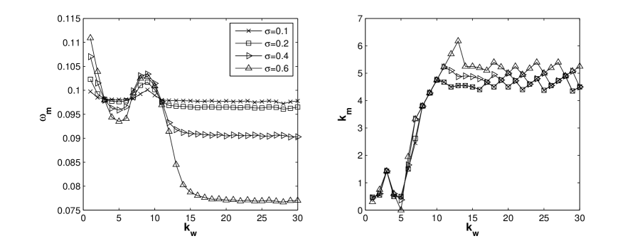

The effect of wall wavenumber on the maximum growth rate is illustrated in the left panel of figure 3 which shows that reaches a local minimum around for that is close to the most unstable mode in the straight tube case. This minimum value is also close to the uncorrugated case when is small. Meanwhile, the growth rate also tends to have a local maximum when . For a larger , this local minimum (maximum) has a smaller (larger) value. The parameter is chosen in figure 3 but other choices of showed qualitatively similar results. For relatively large , varies little and is seen to reach a smaller value for a larger . As will be shown in the nonlinear simulations later, the relatively large leads to a tube with an effective radius . Therefore a larger (with large ) means an effectively narrower tube which enhances the confinement and gives smaller growth rate.
Meanwhile, we investigate the variation of the associated wavenumber at which is obtained in the right panel of figure 3. For most cases, there are two locations where is reached within one period. We only highlight the one within the long wave range or the smaller one. The other one can be calculated easily by using , since is the first wall harmonic of the perturbation. For relatively small , is found to be shifting between a small value close to zero and approximately. Corresponding to the local minimum from the left panel of figure 3, is found in the right panel (for ). Then the other mode is found to approach . For relatively large ( in figure 3), so the other one is close to which indicates an obvious shift in the dominant modes. As increases, also increases until is sufficiently large, where oscillates around 5, which corresponds to the case when the unstable branch from the uncorrugated case has been recovered (see the similar case in the figure 2 for ). But there still exists small deviation in and from the exact value in the uncorrugated straight tube case. Similar deviation phenomenon in and was also pointed out in [75].
In figure 4, we compare the growth rates calculated directly from the long wave model (21), (22) with the results based on the lubrication model (28). In order to make the comparison, is taken and a thin annular layer is considered with . Based on (25), and are used in the full long wave model. Suppose is the growth rate obtained from (28), the true growth rate in the long wave model is calculated as which is plotted in figure 4. Two typical wall wavenumbers are chosen in figure 4, where the agreement is good, although the lubrication model seems to overestimate the growth rate slightly for this value of in the left panel, but in general has predicted the modes associated with the maximum growth rate. In the next section, we carry out direct numerical simulations to further validate the results we obtained for the linear stability.
3.2 Nonlinear evolution

In the results reported here, we consider the wall shape as , with initial and (no axial flux) boundary conditions given by
| (34) | |||
| (35) |
To ensure both the wall and interface are periodic in the computational domain, the period length is taken as where is the common divisor such that with both integers (see also [76]). In addition, , and are fixed in simulation unless otherwise stated. Since is small, the early stage evolution is expected to follow the linear theory which will be confirmed numerically later. The nonlinear equations are solved by the solver EPDCOL [40] which has been successfully used for related problems ([16] e.g.), and our previous studies ([73, 74]). This solver uses the finite element discretization in space and advances in time through the Gear’s method. In the results reported here, about space points are used within the computational domain. The simulation is stopped when the neck of the core thread or the vertical gap between the wall and interface is smaller than , which indicates a touching solution or annular film rupture rather than pinching of the core liquid thread in our problem.


Our numerical results by choosing an initially slightly perturbed thread interface show fair agreement with the linear theory for which we solved by using the FFH method. A few typical results are shown in figure 5. In the panel (a), the evolution is shown for , in which case the growth rate is larger than the straight tube case based on the inset, where the star symbol indicates the parameter values used in simulation. In fact, due to corrugation, the disturbance is modulated by exp () and the eventual dominant growth rate is associated with the mode (first wall harmonic) (or due to the periodicity). It is shown that the interface evolves first as if there were no wall roughness and the growth rate follows the value in the straight tube case, for at early stage. After , the interface recognizes the wall topography effect and then follows the new dominant growth mode that is predicted by our FFH method. The agreement is shown by viewing the solid line from the direct simulation and the dashed line from linear theory agree with each other well, even though in this particular case, the time period showing the agreement is relatively short and the amplitude of the perturbation grows to finite for which the linear theory is not strictly valid. Our results do not indicate that the linear theory is able to predict finite amplitude growth. The agreement merely coincides with the fact that the linear theory usually works well even beyond its valid domain. More details of the interface evolution will be revealed in figure 6. The important message that our numerical results delivered is the existence of the transition (see also the simulations in [75]). It is as expected and can be explained using our (33), which indicates that the growth rate from the uncorrugated case dominates in short times and there exists a critical time when the correction term due to corrugation eventually becomes the same order as . The transition exists for most of cases as long as the growth rate differs from . But it will not appear if the thread experiences breakup before reaching the critical time.
In panel (b) and (c), we fix but choose two different wavenumbers for the initial condition: one corresponds to a mode that is roughly equal to the uncorrugated tube case, while the other one corresponds to a mode that would have been stable if the wall is uncorrugated, . Then it is not surprising that the interface follows a single growth rate from the linear theory in panel (b). In panel (c), we again observe some transient growth first. At early stage, the relatively shortwave perturbation saturates (the growth rate is negative for in the straight tube case) and after , the evolution follows the growth rate from the linear theory for . Panel (d) illustrated a similar case as panel (c) but with a smaller , i.e. the wall is initially closer to the thread interface, which shows qualitatively the same behavior as panel (c). Such transient growth from saturated shortwave perturbations to unstable long wave ones is also observed in [75], in which the annular layer is asymptotically thin and the core dynamics is neglected.
We also carry out a close inspection in the case in panel (a) and (c) of figure 5 by showing the interface profiles in figure 6 and 7 respectively. Corresponding to the case in panel (a) of figure 5, the interface evolves first as the case with no corrugation before which is shown in the panel (a) of figure 6, while the panel (b) shows the evolution after the transition, which, despite the fact that some short waves surf on the large wave crest, follows longer wave length perturbation compared to the initial relatively short wave length perturbation. In particular, the eventual dominant mode is instead of as discussed above. The wall shape is illustrated in the upper panels only in order to view the relative phase between the interface shape and the wall. For the case in panel (c) of figure 5, the transition from stabilizing to destabilizing is obvious. As indicated in figure, we plotted the thread profiles before and after the turning point . In the panel (a) of figure 7, the perturbation is indeed saturated as the amplitude of the perturbation decreases, while in the panel (b), the perturbation is amplified obviously and the core tends to pinch off eventually. This result is in good qualitative agreement with those in [75]. The corresponding evolution of in bottom panel (c) further confirmed this transient evolution, where the circle indicates reached a maximum as time advances.
The dashed lines in the panels (c) of figure 6 and 7 are the results when inertia terms are included in calculations. Similar to the findings in [74], the inertia only affects the transient evolution slightly while having little effect both in the early stage and near pinching. It is also consistent with the scaling analysis in [51] where inertia is shown to give way to viscous fluid-fluid interaction when the region is slender. Therefore, we focus mainly on the Stokes flow problem, i.e. , for the discussion here.
3.3 Drop formation and film drainage
In this subsection, we investigate the drop formation toward the breakup of the liquid threads or layers. In figure 8, drop and satellite formations for various wall shapes are shown when the tube wall is initially far away from the thread interface, , so that the tube wall is out of sight in all the panels (the same tube wall shapes will be shown in figure 9). In the top panels of figure 8, the tube wall is kept uncorrugated, , while with for the following three ones from the top to the bottom. It is seen that the drop formation can be quite different when the wall has wavy structure. In the panels in the second row, corresponds to a point that leads to a larger linear growth rate than the straight tube case (see panel (a) in figure 2), which causes the thread to pinch with fewer large or mother drops than the top panel. The satellite formations are illustrated in the right column of figure 8. In addition, further short-wave perturbation causes the surface of large drop to have dimples. When , the panel (b) of figure 2 shows the linear growth rate dominated by the resonant one which is close to , while , one unstable branch completely covers the growth rate curve in the case of no wall corrugation. Therefore, it is expected that the eventual drop shapes in the third and bottom row are similar to the top panel. However, a close inspection reveals that, although the drop shape is similar, the detail of pinch-off differs. For , the satellites are obtained simultaneously since the actual period is in the top row of figure 8. For and in the third row, the middle satellite is obtained via the first breakup while the rest possible satellites can only appear from the subsequent breaks up (since the necking region has already formed, it is likely they will be the satellite drops; see the related work in [70] which presented a ’self-repeating’ mechanism on a series of breakups to obtain satellites). In the bottom row, the left (right) most satellite together with the middle satellite breakups earlier than the ones next to them. The calculation after the first pinch off may be interesting, but this is beyond the scope of this paper. The difference in droplet sizes (together with the cases having different values of ) will be summarized later in figure 12.

Since the tube wall would appear far away from the local pinching region (assuming the tube cross section variation is not too large), the pinching behavior would be expected to resemble the case with no wall corrugation (see the study on the pinching dynamics in [74]). Therefore this is not pursued further in current work.


When the annular layer is relatively thin, namely, the averaged tube radius is small, we show drop formation for in figure 9, where the wall shapes are chosen to be the same as in figure 8 but they are visible in figure now. In the top two panels, the tube is straight, and we obtain the so called plug-with-collar drop formation (see [32] and [74]) where the fluids are trapped between the tube wall and the large drops along with pinch off. When the tube wall has variation in shape, the thread needs to cope with the wall constraint and larger drops can be expected at first breakup even starting with the same initial perturbation wavenumber. The drop shapes resemble the results in [55] in the full axisymmetric simulations when the wall variation is present. The panels in the second row of figure 9 show larger drops in the middle of the thread compared to the top panels where the tube wall is straight, because a longer wave length perturbation is excited by the wall harmonics, (see also the argument in [75]). In the third row, pinching occurs near , leaving a long thread both at and . Additionally, the left one in the third row would perhaps experience a second breakup due to the thin neck around , which leads to multiple drop formations. Meanwhile, in some portion of the tube, the annular layer tends to breakup as well, since as pinching occurs, the film drainage regime is also approached slowly. Due to the wall topography, it is seen that more fluids compared to the case can be trapped between the wall and drops. In the last row of figure 9, drop formation is seen to differ significantly. In the left panel, a ultimate multiple drop formation is expected, while in the right panel, a large size drop is obtained in the middle which is connected by drops in comparable sizes. As shown later, this case in the right bottom panel stands near a transition from pinching solutions to film rupture solutions.
The associated evolutions of the corresponding minimum thread radius and the minimum thread-tube gap are plotted in figure 10, where the left panel for the case , shows as , i.e. the core thread pinches, the minimum gap still remain significantly larger compared to or at least, decays faster than the gap value. Therefore pinching solutions are obtained (at least up to here). As shown in the thin annulus limit, owing to the different time scales (recall with in (27) and (28)), pinching is expected to occur in advance of film drainage that happens in longer time dynamics, and perhaps even after the first pinch off, as shown in [32] in the straight uncorrugated tube case. In addition, we observe from the left panel of figure 10 that the change in minimum gap along pinching with is not monotonic. It seems that the gap remains larger for than . The right panel of figure 10 shows similar results to the left panel, except that and for sufficiently large (), the neck of core thread remains order one while the gaps seem to reach a very small value first. In those cases, we provided the numerical evidence that a tube wall with large wavenumber may induce the film drainage regime, meanwhile suppress pinching even for a case where the annulus is not asymptotically thin. In the case without wall corrugation, , to suppress pinching, sufficiently thin annulus is required (the numerical work by [54] gave a threshold value for the uncorrugated tube in Stokes flow); in contrast, we found (namely, the average film thickness ) is sufficiently small to produce this phenomenon. In general, this should also depend on the size of wall variation (as well as the initial conditions on the thread profiles). For the discussion here, is fixed all the time and we merely provide the evidence of possible pinching suppression for an annular layer whose thickness is not asymptotically small. Figure 11 shows the thread interface shape at the final stage of our simulations, at and respectively, where it seems that the effective tube radius is reduced () due to the rapid variation of tube cross section, which makes the fluids inside the wall undulation effectively rigid. Notice that in figure 11, the core fluid does not intrude the inside of the wall undulation part, while in figure 9 (the third and fourth row in particular), the core fluid still can wrap around the undulation ’tips’. As the liquid layer keeps thinning, locally, one still expects the lubrication model holds as well as the scaling laws based on it (see [33] and [50], where for a collar next to a collar, for a lobe next to a collar, with the minimum film thickness to the substrate and the time). Unfortunately our numerical results fail to show the scalings even the gap is small and in the order of . It is possible that the thin film regime has not been fully reached yet as the fluid interface is only touching the wall undulation tip and the fluid region adjacent to the thinning part is different from the collar or lobe that is seen in [50].
Finally, for pinching solutions, we show the effect of the wall wavenumber on the breakup times and drop sizes, with the latter characterized by an effective drop radius that is defined as
| (36) |
where are two points associated with sufficiently thin thread neck that we consider to be the pinching points. In the left panel of figure 12, the breakup time first decreases and then increases as varies between and . This is expected from our linear theory (also qualitatively similar to the results in figure 3). When corresponds to a mode with larger growth rate, the breakup time is smaller. For example, when , the dominant mode is for and or for . Accordingly, the growth rate is and respectively, which indicates the former case breakups earlier than the latter one. As increases, increases and the increasing is more profound when is smaller. For , the breakup time eventually approaches the value in the straight tube case for large approximately, because the initial wavenumber is already a long wave one, and one of the unstable branches in the linear theory for has almost covered the straight tube case (see figure 4). While for the relatively small , the annular film also tends to reach the drainage regime which occurs in a longer time scale and tends to suppress the pinching. As given in figure 11, the annular film touching solution is obtained instead of pinching for and the interface profile that is shown is at . The right panel of figure 12 illustrates the distribution of a large and satellite drops. For clarity here, we only calculate the satellite size from the first breakup (typically the one satellite in the middle) together with the adjacent large drops, where we estimated a second pinching point, as our current code can only track down to the first breakup. But for in figure 8, there are clearly three large drops and two small satellites, which are all taken into account. This has also been done for the small cases. For in figure 8, multiple satellite formation is expected eventually, which is similar for (data not shown). As increases, it is seen that the size of both the large and satellite drops increases to a local maximum for some within the range , or , which depends on the value of . The drop sizes are similar to the straight tube case when is relatively large except when is sufficiently small. For , the size of the satellite drop keeps decreasing as increases. Based on our numerical results in figure 10, this indicates a transition from the pinching to touching solution.
4 Concluding remarks
We have studied the effect of wall corrugation on the linear stability and nonlinear dynamics of viscous liquid threads and annular layers inside a cylindrical tube. A long wave model accounting for the wall shape effect, as well as the coupling between the annular layer and an active core thread, has been derived, which, in appropriate limits, reduces to the equations in literature [24, 33, 75, 76, 51]. Similar to the findings in [75], the linear stability of the system shows that the short waves, which would be stable in the uncorrugated tube case, can excite unstable long waves through the interaction with the wall shape variations. When the wall wavenumber is relatively small, along with unstable short waves, the long waves are more unstable, or have larger dominant growth rate, compared to the uncorrugated wall case. Consequently, the breakup time is expected to decrease. A stable band of modes appear when the wall wavenumber is sufficiently large.
The stability of the threads and layers in the nonlinear regime was then investigated via direct numerical simulations of the evolution equations. Starting with relatively small initial perturbation, the results in general agree with our linear theory with a transition period, where the growth first follows the value predicted in the uncorrugated tube problem. Drop formation as well as drop size is shown to alter by including the wall corrugation. Typically, larger and fewer drops can be expected based on the simulation results, by choosing proper parameters and . Meanwhile, similar to the ’plug with collar’ formation (see [32, 74]), accompanied by pinching, fluids are found to be trapped between the tube wall and the core thread, where the film drainage regime is approached and is expected to persist perhaps even after the first pinch off. Furthermore, we showed possibility that pinching solutions can be suppressed depending on the choices of and .
The model here provides a template for further studies or extensions; one can include some external field (gravity, electric field e.g.) or interfacial surfactants, as much remains to be explored. Meanwhile, this reduced model has the advantage over the full problem regarding the computational cost issue.
Furthermore, with this model, other more complicated wall shapes can be incorporated easily, which are related to the engineering design for heat transfer optimization, drug or particle delivery and emulsification (see [72] e.g.) in microfluidic devices and also in biological systems [31, 48]. We already have a few preliminary results underworking on controlling the droplet sizes by changing channel or tube wall shapes. Intuitively for example, liquid thread breaks slower in a tube with smaller radius because of a smaller growth rate. Therefore a combination or a contraction-expansion tube would lead to a series of droplets in the expansion side, when the thread is not broken yet in the contraction or narrow side, which is similar to those ’flow-focusing-device’ ideas to some extent, although the roughness of the wall could potentially complicates the dynamics. Similarly, with locally dimpled tube, different size of droplets can be obtained so that a desired drop distribution may be achieved. Flow rate is another key parameter in the experiments and this will be investigated in the future by inserting axial flow or some external forcing in our model. However, our present work focuses only on the stability of a stationary thread as the axial flow does not affect the real part of our growth rate , of temporal stability. We take this as a first step of modeling to understand the physics of the system and more are under working.
Appendix A Formulation of the linearized problem
In this section, we briefly derive the formulation for calculating the linear growth rate by applying the FFH method. Let and , where is the Bloch wavenumber or Floquet multiplier; then (29) becomes
| (37) |
Multiplying the above equation (37) by and taking the Fourier transform, we obtain the following equation (more details can be found in [20])
| (38) |
with and where
| (39) |
In addition, the bi-infinite matrices are defined by
| (40) |
where or , is the highest number of derivatives in th side and stands for the coefficient function in front of th derivatives and can be represented by a Fourier series
| (41) |
In particular, and for (37), and
| (42) | |||
| (43) |
The spectrum is periodic and only is needed to discuss since larger range gives no more information (see [75] e.g.). To calculate the spectrum numerically, we choose a cut-off on the number of Fourier modes of the eigenfunctions , resulting in a linear system of dimension from (38).
References
- [1] B. Ambravaneswaran, E. D. Wilkes, and O. A. Basaran, Drop formation from a capillary tube: comparison of one-dimensional and two-dimensional analyses and occurrence of satellite drops, Phys. Fluids, 14 (2002), pp. 2606–2621.
- [2] R. W. Aul and W. L. Olbricht, Stability of a thin annular film in pressure-driven, low reynolds-number flow through a capillary, J. Fluid Mech., 215 (1990), pp. 585–599.
- [3] N. J. Balmforth and S. Mandre, Dynamics of roll waves, J. Fluid Mech., 514 (2004), pp. 1–33.
- [4] N. Bermond, A. R. Thiam, and J. Bibette, Decompressing emulsion droplets favors coalescence, Phys. Rev. Lett., 100 (2008), p. 024501.
- [5] P. J. Blennerhassett and A. P. Bossom, The linear stability of high-frequency oscillatory flow in a channel, J. Fluid Mech., 556 (2006), pp. 1–25.
- [6] D. B. Bogy, Drop formation in a circular liquid jets, Annu. Rev. Fluid Mech., 11 (1979), pp. 207–228.
- [7] M. Booty, D. T. Papageorgiou, M. Siegel, and Q. Wang, Long-wave equations and direct numerical simulations for the breakup of a viscous fluid thread surrounded by an immiscible viscous fluid, IMA J. Appl. Math., 78 (2013), pp. 851–867.
- [8] S. Chandrasekhar, Hydrodynamic and hydromagnetic stability, Oxford University Press, UK, 1961.
- [9] A. U. Chen, P. K. Notz, and O. A. Basaran, Computational and experimental analysis of pinch-off and scaling, Phys. Rev. Lett, 88 (2002), pp. 174501–1.
- [10] K. Chen, R. Bai, and D. D. Joseph, Lubricated pipelining. part 3. stability of core-annular flow in vertical tubes, J. Fluid Mech., 214 (1990), pp. 251–286.
- [11] K. Chen and D. D. Joseph, Long waves and lubrication theories for core annular flow, Phys. Fluid A, 3 (1991), pp. 2672–2679.
- [12] Y.-J. Chen and P. H. Steen, Dynamics of inviscid capillary breakup: collapse and pinchoff of a film bridge, J. Fluid Mech., 341 (1997), pp. 245–267.
- [13] G. F. Christopher and S. L. Anna, Microfluidic methods for generating continuous droplet streams, J. Phys. D: Appl. Phys., 40 (2007), pp. R319–R336.
- [14] I. Cohen, M. P. Brenner, J. Eggers, and S. R. Nagel, Two fluid drop snap-off problem: Experiments and theory, Phys. Rev. Lett., 83 (1999), p. 1147.
- [15] R. V. Craster and O. Matar, On viscous beads flowing down a vertical fibre, J. Fluid Mech., 553 (2006), pp. 85–105.
- [16] R. V. Craster, O. Matar, and D. T. Papageorgiou, Pinchoff and satellite formation in surfactant covered viscous threads, Phys. Fluids, 14 (2002), pp. 1364–1376.
- [17] , On compound threads with large viscosity contrast, J. Fluid Mech., 533 (2005), pp. 95–124.
- [18] C. G. Dassor, J. A. Deiber, and A. E. Cassano, Slow two-phase flow through a sinusoidal channel, Intl. J. Multiphase Flow, 10 (1984), pp. 181–193.
- [19] R. F. Day, E. J. Hinch, and J. R. Lister, Self-similarity capillary pinchoff of an inviscid fluid, Phys. Rev. Lett., 80 (1998), pp. 704–707.
- [20] B. Deconinck and J. N. Kutz, Computing spectra of linear operators using the floquet-fourier-hill method, J. Comp. Phys., 219 (2006), pp. 296–321.
- [21] G. F. Dietze and C. Ruyer-Quil, Films in narrow tubes, J. Fluid Mech., 762 (2015), pp. 68–109.
- [22] J. Eggers, Universal pinching of 3d axisymmetric free surface flow, Phys. Rev. Lett, 71 (1993), p. 3458.
- [23] , Nonlinear dynamics and breakup of free-surface flows, Rev. Mod. Phys., 69 (1997), p. 865.
- [24] J. Eggers and T. F. Dupont, Drop formation in a one-dimensional approximation of the navier-stokes equations, J. Fluid Mech., 262 (1994), pp. 205–221.
- [25] J. Eggers and E. Villermaux, Physics of liquid jet, Rep. Prog. Phys., 71 (2008), p. 036601.
- [26] A. L. Frenkel, A. J. Babchin, B. G. Levich, T. Shlang, and G. I. Sivashinsky, Annular flows can keep unstable films from breakup: nonlinear saturation of capillary instability, J. Colloid Interface Sic., 115) (1987), pp. 225–233.
- [27] P. A. Gauglitz and C. J. Radke, The dynamics of liquid film breakup in constricted cylindrical capillaries, J. Colloid INterface Sci., 134 (1990), pp. 14–40.
- [28] E. Georgiou, C. Maldarellii, , D. T. Papageorgiou, and D. S. Rumschitzki, An asymptotic theory for the linear stability of a core-annular flow in the thin annular limit, J. Fluid Mech., 243 (1992), pp. 653–677.
- [29] S. L. Goren, The instability of an annular thread of fluid, J. Fluid Mech., 12 (1962), pp. 309–319.
- [30] , The shape of a thread of liquid undergoing break-up., J. Colloid Sci, 19 (1964), pp. 81–86.
- [31] J. B. Grotberg, Respiratory fluid mechanics, Phys. Fluids, 23 (2011), p. 021310.
- [32] J. G. Hagedorn, N. S. Martys, and J. F. Douglas, Breakup of a fluid thread in a confined geometry: droplet-plug transition, perturbation sensitivity, and kinetic stabilization with confinement, Phys. Rev. E, 69 (2004), p. 056312.
- [33] P. S. Hammond, Nonlinear adjustment of a thin annular film of viscous fluid surrounding a thread of another within a circular cylindrical pipe, J. Fluid Mech., 137 (1983), pp. 363–384.
- [34] C. E. Hickox, Instability due to viscosity and density stratification in axisymmetric pipe flow, Phys. Fluid, 14 (1971), pp. 251–262.
- [35] H. H. Hu and D. D. Joseph, Lubricated pipelines: Stability of core-annular flow. part 2., J. Fluid Mech., 205 (1989), pp. 359–396.
- [36] H. H. Hu, T. Lundgren, and D. D. Joseph, Stability of core-annular flow with small viscosity ratio, Phys. Fluid A, 2 (1990), pp. 1945–1954.
- [37] K. J. Humphry, A. Ajdari, A. Fernandez-Nieves, H. A. Stone, and D. A. Weitz, Suppression of instabilities in multiphase flow by geometric confinement, Phys. Rev. E, 79 (2009), p. 56310.
- [38] D. D. Joseph, R. Bai, K. P. Chen, and Y. Y. Renardy, Core-annular flows, Annu. Rev. Fluid Mech., 29 (1997), pp. 65–90.
- [39] S. Kalliadasis and H.-C. Chang, Drop formation during coating of vertical fibres, J. Fluid Mech., 261 (1994), pp. 135–168.
- [40] P. Keast and P. H. Muir, Algorithm 688 epdcol – a more efficient pdecol code, ACM Trans. Math. Softw., 17 (1991), p. 153.
- [41] V. Kerchman, Strongly nonlinear interfacial dynamics in core-annular flows, J. Fluid Mech., 290 (1995), pp. 131–166.
- [42] C. Kouris and J. Tsamopoulos, Concentric core-annular flow in a periodically constricted circular tube. part 1. steady-state, linear stability and energy analysis, J. Fluid Mech., 432 (2001), pp. 31–68.
- [43] , Dynamics of axisymmetric core-annular flow in a straight tube. i. the more viscous fluid in the core, bamboo waves, Phys. Fluid, 13 (2001), pp. 841–858.
- [44] , Dynamics of the axisymmetric core-annular flow. ii. the less viscous fluid in the core, saw tooth waves, Phys. Fluid, 14 (2002), pp. 1011–1029.
- [45] T.A. Kowalewski, On the separation of droplets from a liquid jet, Fluid Dyn. Res., 17 (1996), pp. 121–145.
- [46] H. C. Lee, Drop formation in liquid jets, IBM J. Res. Develop., 18 (1971), pp. 364–369.
- [47] D. Leppinen and J. R. Lister, Capillary pinch-off in inviscid fluids, Phys. Fluid, 15 (2003), pp. 568–578.
- [48] R. Levy, D. B. Hill, M. G. Forest, and J. B. Grotberg, Pulmonary fluid flow challenges for experimental and mathematical modeling, Integr. Comp. Biol., 54 (2014), pp. 985–1000.
- [49] D. R. Link, S. L. Anna, D. A. Weitz, and H. A. Stone, Geometrically mediated breakup of drops in microfluidic devices, Phys. Rev. Lett., 92 (2004), p. 054503.
- [50] J.R. Lister, J.M. Rallison, A.A. King, L.J. Cummings, and O.E. Jensen, Capillary drainage of an annular film: the dynamics of collars and lobes, J. Fluid Mech., 552 (2006), pp. 311–343.
- [51] J. R. Lister and H. A. Stone, Capillary breakup of a viscous thread surrounded by another viscous fluid, Phys. Fluids, 10 (1998), p. 2758.
- [52] G. H. McKinley and A. Tripathi, How to extract the newtonian viscosity from capillary breakup measurements in a filament rheometer, J. Rheol., 44 (2000), p. 653.
- [53] M. Muradoglu and A. D. Kayaalp, An auxiliary grid method for computations of multiphase flows in complex geometries, J. Comp. Phys., 214 (2006), pp. 858–877.
- [54] L. A. Newhouse and C. Pozrikidis, The capillary instability of annular layers and liquid threads, J. Fluid Mech., 242 (1992), pp. 193–209.
- [55] U. Olgac, A. D. Kayaalp, and M. Muradoglu, Buoyancy-driven motion and breakup of viscous drops in constricted capillaries, Int. J. Multiphase Flow, 32 (2006), pp. 1055–1071.
- [56] D. T. Papageorgiou, Stability of unsteady viscous flow in a curved pipe, J. Fluid Mech., 182 (1987), pp. 209–233.
- [57] , Analytical description of the breakup of liquid jets, J. Fluid Mech., 301 (1995), pp. 109–132.
- [58] , On the breakup of viscous liquid threads, Phys. Fluids, 7 (1995), pp. 1529–1544.
- [59] D. T. Papageorgiou, C. Maldarelli, and D. S. Rumschitzki, Nonlinear interfacial stability of core-annular film flows, Phys. Fluids A, 2(3) (1990), p. 340.
- [60] C. Pozrikidis, Capillary instability and breakup of a viscous thread, J. Eng. Math, 36 (1999), pp. 255–275.
- [61] L. Preziosi, Chen K, and D. D. Joseph, Lubricated pipelines: stability of flow, J. Fluid Mech., 201 (1989), pp. 323–356.
- [62] T. C. Ransokoff, P. A. Gauglitz, and C. J. Radke, Snap-off of gas bubbles in smoothly constricted noncircular capillaries, AIChE J., 33 (1987), pp. 753–765.
- [63] Lord Rayleigh, On the instability of jets, Proc. Lond. Math. Soc., 10 (1878), pp. 4–13.
- [64] M. Renardy, Some comments on the surface-tension driven breakup (or lack of it) of viscoelastic jets, J. Non-Newtonian Fluid Mech., 51 (1994), pp. 97–102.
- [65] , A numerical study of the asymptotic evolution and breakup of newtonian and viscoelastic jets, J. Non-Newtonian Fluid Mech., 59 (1995), pp. 267–282.
- [66] A. Rothert, R. Richter, and I. Rehberg, Formation of a drop: viscosity dependence of three flow regimes, New J. Phys, 5 (2003), pp. 59.1–59.13.
- [67] S. Saprykin, R. J. Koopmans, and S. Kalliadasis, Free-surface thin-film flows over topography: influence of inertia and viscoelasticity, J. Fluid Mech., 578 (2007), pp. 271–293.
- [68] X. D. Shi, M. P. Brenner, and S. R. Nage, A cascade of structure in a drop falling from a faucet, Science, 265 (1994), pp. 219–222.
- [69] A. Sierou and J. R. Lister, Self-similar solutions for viscous capillary pinch-off, J. Fluid Mech., 497 (2003), pp. 381–403.
- [70] M. Tjahjadi, H. A. Stone, and J. M. Otino, Satellite and subsatellite formation in capillary breakup, J. Fluid Mech., 243 (1992), pp. 297–317.
- [71] S. Tomotika, On the instability of a cylindrical thread of a viscous liquid surrounded by another viscous fluid., Proc. Roy. Soc. A, 150 (1935), pp. 322–337.
- [72] A. S. Utada, E. Lorenceau, D. R. Link, P. D. Kaplan, H. A. Stone, and D. A. Weitz, Monodisperse double emulsions generated from a microcapillary device., Science, 308 (2005), pp. 537–541.
- [73] Q. Wang, Breakup of a viscous poorly conducting liquid thread subject to a radial electric field at zero reynolds number, Phys. Fluid, 24 (2012), p. 102102.
- [74] , Capillary instability of a viscous liquid thread in a cylindrical tube, Phys. Fluid, 25 (2013), p. 112104.
- [75] H-H Wei and D. S. Rumschitzki, The linear stability of a core-annular flow in an asymptotically corrugated tube, J. Fluid Mech., 466 (2002), pp. 113–147.
- [76] , The weakly nonlinear interfacial stability of a core-annular flow in a corrugated tube, J. Fluid Mech., 466 (2002), pp. 149–177.
- [77] E. D. Wilkes, S. D. Phillips, and O. A. Basaran, Computational and experimental analysis of dynamics of drop formation, Phys. Fluids, 11 (1999), pp. 3577–3598.