Stability analysis of admittance control
using asymmetric stiffness matrix
Abstract
In contact-rich tasks, setting the stiffness of the control system is a critical factor in its performance. Although the setting range can be extended by making the stiffness matrix asymmetric, its stability has not been proven. This study focuses on the stability of compliance control in a robot arm that deals with an asymmetric stiffness matrix. It discusses the convergence stability of the admittance control. The paper explains how to derive an asymmetric stiffness matrix and how to incorporate it into the admittance model. The authors also present simulation and experimental results that demonstrate the effectiveness of their proposed method.
I Introduction
In-demand automation tasks often involve contact-rich tasks with varying mechanical constraints between the robot and the environment, making control program implementation complex. Studies on contact-rich tasks using the peg-in-hole benchmark have expanded automation technology, particularly for precision assembly. Compliance mechanisms, such as active and passive compliance, help robots to perform assembly tasks despite positional errors. Impedance and admittance control are common methods for active compliance [1, 2]. Contact-model-based [3, 4] and contact-model-free [5, 6] approaches are used for compliance control, with the latter often using machine learning methods such as learning from demonstration and learning from the environment with reinforcement learning.
Variable impedance control (VIC), a control strategy that adjusts a robot’s mechanical impedance for safe, versatile, and efficient interaction, has been actively studied [7]. VIC has shown promising results in various applications, such as manipulation, locomotion, haptic feedback, and rehabilitation. However, it faces several challenges, such as the design of robust and efficient actuators and sensors, as well as the development of effective control strategies for complex and dynamic tasks [8].
Methods that use passive compliance obtain the desired stiffness of the hand by using a device that combines passive mechanical elements such as springs. The remote center compliance (RCC) device is one of the most popular examples, which utilizes the inter-axis interference to induce motion against external force [9]. Instead of VIC, variable RCC (VRCC), which can set stiffness in a variable manner, has been studied to deal with complicated tasks [10, 11].
RCC has the advantage of not being limited by control bandwidth because it is composed of mechanical elements. On the other hand, when compliance is reproduced by control, even ranges that cannot be reproduced mechanically can be artificially reproduced with a single parameter setting. In other words, the compliance control has a wider range over which motion can be induced. However, how to set the parameters under an assurance of stability is an important issue.
A passivity-based approach is the most popular candidate to ensure the stability of VIC [12]. It has also been extended to the time-varying admittance controller [13]. Kronander and Billard proposed stability conditions for the VIC scheme that works for different levels of stiffness and damping, using a modified Lyapunov function [14]. Later, Sun et al. expanded on this idea and proposed new constraints that ensure both exponential stability and boundedness of the robot’s position, velocity, and acceleration [15]. Spyrakos-Papastavridis et al. proposed a Passivity-Preservation Control (PPC) that enables the implementation of stable VIC and provided joint and Cartesian space versions of the PPC controller permit the intuitive definition of interaction tasks [16]. In the study of parameter design for variable admittance control, Kim and Yang performed a stability analysis based on the root locus [17]. The root locus has also been used in the parameter design for drill admittance control [18].
While many stability analyses of compliance control have been conducted, only passivity-based analysis has been pursued in multi-degree-of-freedom systems because the problem becomes complex due to the consideration of interference in other axes [19]. Previous studies on compliance control, such as [20] and [21], have indicated that introducing an asymmetric stiffness matrix can increase the robot’s capability and extend the range of motion induction. However, the main challenge is that the asymmetric part fails to satisfy passivity, making it impossible to ensure stability. In this study, we derived parameters for the stability limit of the asymmetric stiffness matrix based on the eigenvalues of the system matrix. We then demonstrate that stability can be guaranteed by setting the parameters using the root locus method.
The contributions of this paper can be summarized as follows.
-
1.
Spiral oscillations can be excited when the stiffness matrix is asymmetric. We have clarified the condition for such excitation. We also showed that the condition for the absence of spiral oscillation is equivalent to the condition that the eigenvalues of the stiffness matrix are real numbers.
-
2.
We have demonstrated that it is difficult to satisfy the passivity when the above conditions are not satisfied and therefore identified the conditions under which vibration converges using the root locus method.
II Basic Principle
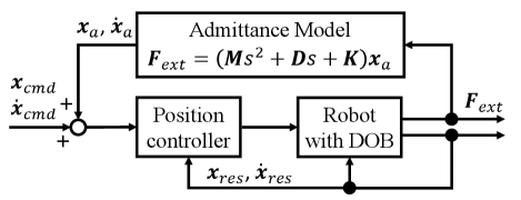
This study discusses the stability of compliance control in a robot arm that deals with an asymmetric stiffness matrix. It is limited to admittance control and discusses the convergence stability of a planar admittance model, assuming the inner position control loop is stable. The feedback control system is shown in Fig. 1. It is an admittance control system with a minor feedback loop for position control. The type of position control is not specified, but a control system using a disturbance observer (DOB) is adopted in the experimental setup. The admittance model is based on the following equation:
| (1) |
This admittance model takes force as input and outputs the position and velocity obtained through numerical integration based on the acceleration obtained from equation (1). While symmetric matrices are typically used for the stiffness matrix and damping matrix of the admittance model, this study considers the use of an asymmetric matrix for the stiffness matrix . For simplicity, the damping matrix is assumed to be a diagonal matrix.
When an external force occurs, the direction in which the robot end effector is induced, and the convergence point are determined only by the stiffness matrix of the admittance model. Therefore, it is desirable to expand the selection range of the stiffness matrix when designing the relationship between external forces and robot operation. On the other hand, since the damping matrix does not affect the convergence point of the end effector, the priority of expanding the selection range is not high. Additionally, applying viscous force only in the direction in which velocity is generated increases the dissipation of energy and is reasonable for enhancing stability. Therefore, it is necessary to consider how to give the diagonal elements of the damping matrix when the non-diagonal elements of the stiffness matrix are given arbitrarily.
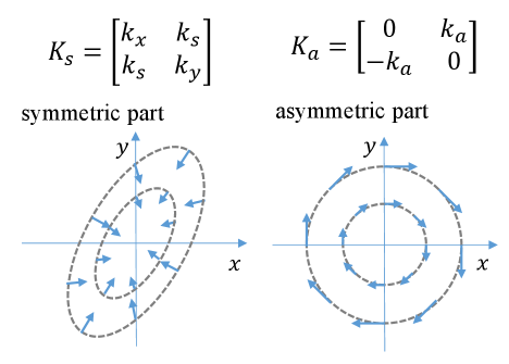
When the stiffness matrix is asymmetric, it is known that the effect of the stiffness matrix can be expressed as a superposition of the symmetric part , which creates a force field that converges at the equilibrium point [1], and the asymmetric part , which creates a force that rotates around the equilibrium point. An example of this is shown in Fig. 2. If the stiffness control is reproduced by a virtual spring, the symmetric part can be treated as generating an elliptical virtual potential energy field generated by strain. Similarly, virtual kinetic energy can be derived from the mass and velocity of the admittance model. Therefore, in the symmetric matrix, a control system design based on passivity can be achieved by deriving an energy function. However, when this is extended to an asymmetric matrix, the curl field generated by the asymmetric part is not a conservative force, and it may excite oscillations. Oscillations excited by the curl field are referred to as spiral oscillations. Since energy may increase due to spiral oscillation, passivity may not be satisfied.
This is demonstrated by the energy function. It is obtained as the integral of the product of velocity and force, which is power.
| (2) |
By substituting and (1) into (2),
| (3) | |||||
| (4) |
Eq. (4) shows that the virtual energy of the admittance model is defined as a function divided into four terms: kinetic energy, stiffness energy, energy loss due to friction, and energy imparted by the asymmetric part. The first and second terms represent kinetic and potential energy, respectively. The third term represents energy dissipated by viscosity, while the fourth term represents energy imposed by the curl field. Since the first and second terms are the energy of conservative forces, if the third term is smaller than the fourth term, the energy function does not increase. However, the above equation depends on velocity, and when the velocity decreases, the dissipative term becomes smaller. Therefore, if there are periods during vibration where the velocity becomes small, passivity may not hold.
III Stability analysis using root locus
The fundamental principle of admittance control described in the previous section shows that it is generally difficult to establish passivity when the stiffness matrix is made asymmetric. Therefore, the stability will be analyzed based on the concept of root locus below. First, the admittance parameters are defined in the x-y plane as follows:
| (5) |
we define the state vector as , then its state equation can be obtained as follows:
| (6) |
Here, . and are the damper and mass of the admittance model. and represent the diagonal elements of the stiffness matrix in the x and y directions, respectively, and and represent the symmetric and asymmetric components of the non-diagonal terms, respectively. Moreover, we define parameters as follows: , then we can write , the system matrix of the state equation, as follows:
| (7) |
The eigenvalues of the system matrix are obtained as follows:
| (8) |
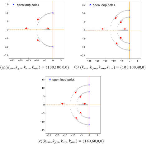
The poles of the transfer function of this admittance model have the same values as the eigenvalues of the system matrix . Therefore, the root locus can be obtained by sweeping a parameter of matrix from 0 to infinity. When the non-diagonal element of the stiffness matrix is zero, i.e., when the stiffness matrix is symmetric, the root locus for varying the damping ratio from 0 to infinity is shown in Fig. 3. For a symmetric matrix, the roots of the natural vibrations, which depend on the stiffness matrix, appear on the imaginary axis, and as the viscous damping ratio increases, the roots move in the negative real axis direction. At the same time, the imaginary part of the root decreases. The damping ratio where the imaginary part of the two conjugate eigenvalues shrinks to zero is called the critical damping ratio. The contents of the square root of (8) are then zero, hence the critical damping ratio is derived by the following equation.
| (9) |
When the value is equal to the critical damping ratio, the roots coincide on the real axis. When the viscous damping ratio increases beyond this value, the roots separate and move to the left and right along the real axis.
Fig. 3(a) shows the result when and , and the stiffness matrix is diagonal. On the other hand, Fig. 3(b) shows the result when and . In other words, the stiffness matrix is not diagonal and its eigenvalues are 140 and 60. Fig. 3(c) shows the result for the case of a diagonal stiffness matrix with the same eigenvalues as in Fig. 3(b), with . The initial position of the root locus changes depending on the eigenvalues of the stiffness matrix, as shown in the comparison of Figs. 3(a), (b), and (c).
In Fig. 3(a), since the two eigenvalues coincide, the root locus starts from the points on the imaginary axis, while in Fig. 3(b), the root locus is split into two upper and lower branches due to the different eigenvalues. Figs. 3(b) and (c) also show that the root locus coincides when the eigenvalues are the same. Eq. (1) deals with a generalized stiffness matrix in two dimensions, but to simplify the derivation of the equation, is set to 0, and stability analysis is performed below. For the case where is not 0, the same root locus can be obtained by deriving its eigenvalues and substituting them into the diagonal elements.
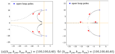
The root locus of the asymmetric matrix is shown in Fig. 4, where four roots appear symmetrically across the imaginary axis when is 0. As is gradually increased from 0, the four roots move negatively along the real axis while the imaginary axis component decreases. As is further increased, two of the four roots change their orientation toward the positive direction of the real axis, and the other two roots move in opposite directions, one positive and one negative. In this case, the imaginary axis component remains slightly. This means that in the case of an asymmetric matrix, oscillations are excited due to the presence of the curl field. However, there is a condition for the parameter that excites the oscillation. To ensure that all eigenvalues are real, it is necessary for the contents of the square root in the second term of the numerator in (8) to be positive, that is,
| (10) |
And it is necessary to have a real value of in (10). To ensure this, the square root term in (10) must be positive. The condition is expressed by the following inequality.
| (11) |
Consequently, condition for the asymmetric element is determined as follows:
| (12) |
If the above inequality is satisfied, the oscillation will no longer occur when is greater than the critical damping. The eigenvalues of the stiffness matrix are derived by the following equation:
| (13) |
The condition for the stiffness matrix to obtain critical damping is equivalent to the matrix having real eigenvalues, as shown by the fact that the condition for (13) to have real solutions is the same as that for (12).
Next, we will derive the conditions for the admittance parameters that ensure stability. If the viscous damping coefficient is increased to a certain value or more, all the roots will move toward the left half of the complex plane, making it possible to stabilize the control system. From (8), in the case of an asymmetric matrix,
| (14) |
The above condition results in the occurrence of positive eigenvalues and unstable poles. However, if , there are no solutions that satisfy (14) for . Therefore, the condition for unstable poles to occur within the range of needs to be investigated. To simplify the (8), are defined as follows:
| (15) |
Then, the eigenvalues are expressed as follows:
| (16) |
Let the real part and imaginary part of be and , respectively, then
| (17) |
Consequently, , and are obtained. By the following equation: , real part is expressed as below:
| (18) |
In order to avoid unstable poles, it is necessary for all eigenvalues to be negative, so we only consider the case where .
| (19) |
The condition that satisfies the (10) is derived below. First, consider the typical case where the equation is simplified, which is . Substituting , into (19) and the following equation is obtained:
| (20) |
If the value of is greater than , then the lower limit of also increases. These parameters are determined by the mass ratio, and to convert them into actual admittance parameters, we substitute , and into the above equation, yielding the following equation:
| (21) |
The next is to consider the case where to further generalize (20) and (21). The condition is still given by (15), but now we substitute the more generalized (10). It is difficult to algebraically derive the condition for all eigenvalues to be negative. However, if (20) is satisfied, then all eigenvalues will be negative.
The proof is shown below. If (19) is satisfied and without changing the values of the other parameters, let us increase the value of from . If in (18) does not increase during this process, (15) will always be satisfied. When differentiating (18) with respect to and , we obtain the following expressions:
| (22) | |||||
| (23) |
when and , both partial derivatives are positive. As (15) shows, increasing always results in a decrease in both and , so the value of in (18) must always decrease. Therefore, if (20) is satisfied, then for all , all eigenvalues are always negative. Replacing and in (20) as follows:
| (24) |
By performing the same equation expansion as above, stability can also be demonstrated for the case where .
IV Simulation study of convergence
IV-A Comparison of time response
A simulation study on the convergence of the proposed method’s root locus was conducted to examine its relationship with stability. An external force of was step-inputted to the admittance model on a 2D plane at equilibrium. The damping coefficient was derived as follows and a comparative study was conducted while changing the value of the damping ratio .
| (25) |
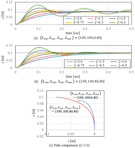
Fig. 5(a) illustrates the simulation results conducted under the same conditions as those in Fig. 4(b). The convergence of the system is determined by the satisfaction of (21). As the damping ratio increases, the magnitude of oscillation decreases. Additionally, the system’s time constant decreases beyond a certain value of . However, oscillation persists even when exceeds 1, and the system did not attain critical damping. Fig. 5(b) shows the results of the same conditions as Fig. 4(b). As the viscosity ratio increases, the oscillation becomes smaller, and the time constant becomes lower. Critical damping occurs at , and no oscillation occurs at higher viscosity ratios. The difference between the two conditions is whether (12) is satisfied or not. Fig. 5(a) has eigenvalues with imaginary components, while Fig. 5(b) does not. The results support the theory that the presence of imaginary components in the eigenvalues of the stiffness matrix determines whether the asymmetric matrix causes spiral oscillations. Since the stiffness matrix in Fig. 5(b) only has positive real eigenvalues, oscillations can be avoided by setting an appropriate viscosity ratio . Fig. 5(c) compares the paths when . It shows that the asymmetric matrix with eigenvalues with imaginary components generated a spiral path, while the matrix with eigenvalues without imaginary components did not cause spiral oscillation.
IV-B Simulation-based validation of passivity
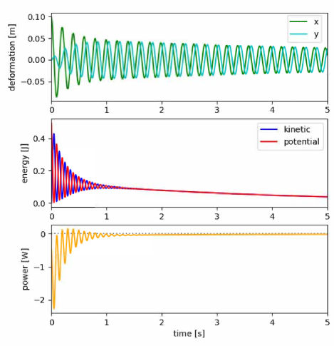
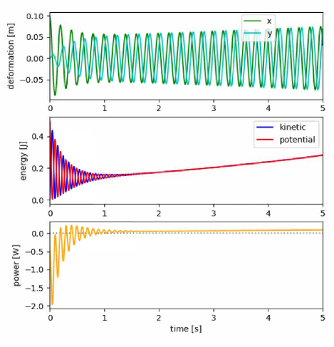
The proposed stability analysis method, which utilizes root locus, provides proof of convergence for a particular parameter range. The stability of compliance control is often shown not only by nominal stability, which does not consider contact with the target, but also by combined stability with contact with the target. Therefore, in this simulation, we reproduced a situation in which the object is fixed to a rigid wall. To illustrate this, we compare the time responses of two simulations in Figs. 6 and 7, with the parameters listed in Table I. The parameters of the admittance model are presented in Table I. A damping value of , which is slightly above the threshold value () derived in (21), caused the system to start oscillating at the mechanical natural frequency and gradually decrease its amplitude, as depicted in Fig. 4. By setting the damping value to , slightly below the threshold value (), the amplitude of the system gradually increased, as shown in Fig. 7. This result demonstrates the validity of (21). Fig. 6 shows stable convergence, and the sum of kinetic energy proportional to the mass and potential energy proportional to the stiffness of the admittance model gradually decreased. However, between 0 and 1 second, there were several time periods when the sum of the outputs was slightly above 0. The increase in energy occurred during periods of low velocity during oscillation. This means that if the loss due to viscous resistance is smaller than the increase in energy due to the curl field, the energy may increase locally even when the amplitude is monotonically decreasing. The system does not satisfy local passivity when the velocity is small. However, the energy only increases in certain phases during oscillation, and final convergence is guaranteed if (21) is satisfied.
| mass | 0.1 | [kg] | stiffness | 100.0 | [N/m] | ||
| sampling | 1 | [ms] | 100.0 | [N/m] | |||
| time | 0.0 | [N/m] | |||||
| 10.0 | [N/m] |
To confirm the validity of the design value of the minimum damper derived in (20), a simulation evaluation was performed: 5 seconds tests were conducted using the same parameters as in Table I. We repeated the test with and changed in the range of -80 to 80. The response was recorded when was varied in increments of 0.1 for each condition, and stability was considered to be maintained when the average kinetic energy for 0.1 seconds was less than 0.2 J at the end of the test. The minimum value of at which this was the case was plotted.
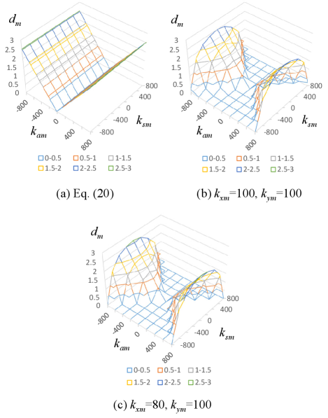
Fig. 8(a) shows the design value derived from (20), and (b) shows the result derived from the above simulation. In all conditions, the control system was confirmed to be stable at a damper below the design value. When is 0, the design value and the simulation results almost coincide, while the larger the absolute value of , the smaller the damper becomes. Eq. (11) shows that the imaginary component of the eigenvalue decreases with increasing absolute value of . Since the imaginary component of is the cause of spiral oscillation, this simulation result confirms the contents of (11). In addition, the region where stability is ensured even when is zero and the region represented by (12) are almost identical. This confirms the validity of (12) as an expression for the parameter region where spiral oscillation does not occur. Fig. 8(c) represents the result when only is changed to 80. As shown in (24), this result confirms that when either stiffness is low, it is desirable to set the parameters according to the higher stiffness value.
The conditions in (12) and (24) only concern the parameter settings for the asymmetric part. Note that other conditions that must be satisfied by the symmetrical part, as indicated in previous studies, must be taken into account. For example, Fig. 8(b) does not show the results for of 1000, but when exceeds 1000, one of the eigenvalues of the symmetric part becomes negative and stability is not satisfied. In sum, it is necessary to design the asymmetric part in addition to the design of the symmetric part in the conventional methods.
V Experiment
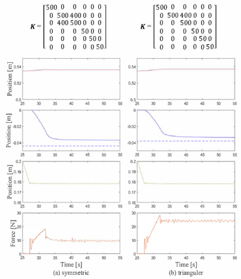
In this experiment, the robot’s performance was evaluated based on the admittance parameter. The robot was made to move vertically towards a metallic board and follow the surface in the y-axis using the displacement caused by the admittance control. Symmetric and asymmetric stiffness matrices were chosen, and damping parameters were set to which was higher than the threshold (). The results shown in Fig. 9 revealed that after contacting the board at seconds, the robot moved towards the negative direction in the y-axis. There was no noticeable movement in the x-axis due to the design of the non-diagonal element of the stiffness matrix. In the case of the symmetric matrix, the difference between the desired displacement and the actual displacement was 8 mm. Due to the setting of , there was slight displacement in the z-axis, which led to a lower contact force . However, in the case of the asymmetric (triangular) matrix, the difference between the desired displacement and the actual displacement was 6 mm, which is shorter than that of the symmetric matrix. Additionally, the contact force was maintained higher because the displacement mainly occurred in the y-axis.
VI Conclusion
This paper discusses the stability of admittance control of a robot arm handling an asymmetric stiffness matrix. Although the introduction of asymmetric elements does not guarantee passivity, it is possible to derive a range of parameters for which stability is guaranteed from the eigenvalues of the system matrix. In addition, the introduction of asymmetric elements may excite helical oscillations, so that critical damping may not be obtained for any given damping parameter, depending on the setting of the stiffness matrix. In this study, we focused on the fact that the spiral oscillation is caused by the imaginary component of the system matrix and clarified the condition of the asymmetric matrix for which critical damping can be obtained. From the simulation and experimental results, it is confirmed that the asymmetric matrix setting method is effective to obtain critical damping. The analysis was performed on a 2-dimensional plane, but future work should extend the theory to a wider range of conditions. The theory can be generalized to systems with three or more degrees of freedom and by utilizing the concept of energy tanks, conduct stability analysis similar to a passive system. The theory may also be extended to variable stiffness control.
References
- [1] N. Hogan, “Impedance control: An approach to manipulation: Part III— Applications,” J. Dyn. Syst., Meas., Control, vol. 107, pp. 121–128, 1985.
- [2] W. S. Newman: “Stability and performance limits of interaction controllers,” Journal of Dynamic Systems, Measurement, and Control, vol. 114, no. 4, pp. 563–570, 2012.
- [3] T. Tang, H. Lin, Y. Zhao, W. Chen, and M. Tomizuka: “Autonomous alignment of peg and hole by force/torque measurement for robotic assembly,” in Proc. 2016 IEEE Int. Conf. on Automation Science and Engineering (CASE), pp. 162–167, 2016.
- [4] H. Unten, S. Sakaino and T. Tsuji: “Peg-in-Hole Using Transient Information of Force Response,” in IEEE/ASME Trans. Mechatronics, vol. 28, no. 3, pp. 1674–1682, 2023.
- [5] S. Gubbi, S. Kolathaya, and B. Amrutur: “Imitation learning for high precision peg-in-hole tasks,” in Proc. of 6th International Conference on Control, Automation and Robotics (ICCAR), pp. 368–372, 2020.
- [6] J. Luo, E. Solowjow, C. Wen, J. A. Ojea, A. M. Agogino, A. Tamar, and P. Abbeel: “Reinforcement learning on variable impedance controller for high-precision robotic assembly,” in Proc. of International Conference on Robotics and Automation (ICRA), pp. 3080–3087, 2019.
- [7] R. Ikeura and H. Inooka: “Variable impedance control of a robot for cooperation with a human,” in Proc. 1995 IEEE Int. Conf. on Robotics and Automation, pp. 3097–3102 vol. 3, 1995.
- [8] F. J. Abu-Dakka and M. Saveriano: “Variable impedance control and learning—a review.” Frontiers in Robotics and AI, vol. 7, 590681, 2020.
- [9] D. E. Whitney: “Quasi-static assembly of compliantly supported rigid parts,” Journal of Dynamic Systems Measurement and Control-transactions of the Asme, vol. 104, pp. 65–77, 1982.
- [10] F. Zhao and P. S. Y. Wu: “VRCC : a variable remote center compliance device,” Mechatronics, vol. 8, no. 6, pp. 657–672, 1998.
- [11] S. Lee: “Development of a new variable remote center compliance (VRCC) with modified elastomer shear pad (ESP) for robot assembly,” IEEE Trans. on Automation Science and Engineering, vol. 2, pp. 193–197, 2005.
- [12] F. Ferraguti, C. Secchi, and C. Fantuzzi: “A tank-based approach to impedance control with variable stiffness,” in Proc. IEEE Int. Conf on robotics and automation pp. 4948–4953, 2013
- [13] F. Ferraguti, N. Preda, A. Manurung, M. Bonfe, O. Lambercy, R. Gassert, R. Muradore, P. Fiorini, and C. Secchi: “An energy tank-based interactive control architecture for autonomous and teleoperated robotic surgery,” IEEE Trans. on Robotics, vol. 31, no. 5, pp. 1073–1088, 2015.
- [14] K. Kronander and A. Billard: “Learning compliant manipulation through kinesthetic and tactile human-robot interaction,” IEEE Transactions on Haptics, vol. 7, no. 3, pp. 367–380, 2014.
- [15] T. Sun, L. Peng, L. Cheng, Z. G. Hou and Y. Pan: “Stability-Guaranteed Variable Impedance Control of Robots Based on Approximate Dynamic Inversion,” in IEEE Transactions on Systems, Man, and Cybernetics: Systems, vol. 51, no. 7, pp. 4193–4200, 2021, doi: 10.1109/TSMC.2019.2930582.
- [16] E. Spyrakos-Papastavridis, P. R. N. Childs, and J. S. Dai: “Passivity Preservation for Variable Impedance Control of Compliant Robots,” in IEEE/ASME Trans. on Mechatronics, vol. 25, no. 5, pp. 2342–2353, 2020, doi: 10.1109/TMECH.2019.2961478.
- [17] H. Kim, W. Yang: “Variable Admittance Control Based on Human–Robot Collaboration Observer Using Frequency Analysis for Sensitive and Safe Interaction,” Sensors, vol. 21, no. 5, 1899, 2021.
- [18] Y. Aydin, D. Sirintuna, C. Basdogan: “Towards collaborative drilling with a cobot using admittance controller,” Trans. Institute of Measurement and Control. vol. 43, no. 8, pp. 1760–1773, 2021.
- [19] C. Ott, A. Dietrich, and A. Albu-Schäffer: “Prioritized multi-task compliance control of redundant manipulators,” Automatica, vol. 53, pp. 416–423, 2015.
- [20] M. Oikawa, T. Kusakabe, K. Kutsuzawa, S. Sakaino, and T. Tsuji: “Reinforcement learning for robotic assembly using non-diagonal stiffness matrix,” IEEE Robotics and Automation Letters, vol. 6, no. 2, pp. 2737–2744, 2021.
- [21] S. Kozlovsky, E. Newman, and M. Zacksenhouse, “Reinforcement Learning of Impedance Policies for Peg-in-Hole Tasks: Role of Asymmetric Matrices,” IEEE Robotics and Automation Letters, vol. 7, no. 4, pp. 10898–10905, 2022.
- [22] K. Ohnishi, M. Shibata, and T. Murakami: “Motion control for advanced mechatronics,” IEEE/ASME Trans. on Mechatronics, vol. 1, no. 1, pp. 56–67, 1996.
- [23] S. W. Doebling, L. D. Peterson, and K. F. Alvin. “Experimental determination of local structural stiffness by disassembly of measured flexibility matrices.” J. Vib. Acoust., vol. 120, no. 4, pp. 949–957, 1998.
- [24] E. Masehian and S. Ghandi: “Assembly sequence and path planning for monotone and nonmonotone assemblies with rigid and flexible parts,” Robotics and Computer-Integrated Manufacturing, vol. 72, 2021, 102180.
- [25] J. E. Colgate and N. Hogan: “Robust control of dynamically interacting systems,” Int. J. Control, vol. 48, no. 1, pp. 65–88, 1988