key
SStaGCN: Simplified stacking based graph convolutional networks
Abstract
Graph Convolutional Networks (GCNs) are powerful models extensively studied for various graph-structured data learning tasks. However, designing GCNs that effectively mitigate the over-smoothing phenomenon remains a crucial challenge. In this paper, we propose a novel Simplified Stacking-based GCN (SStaGCN) framework, leveraging stacking and aggregation techniques to address different types of graph-structured data. Specifically, we first employ stacking base models to extract node features from the graph. Next, we apply aggregation methods—such as mean, attention, and voting techniques—to further enhance feature extraction capabilities. These refined node features are then fed into a vanilla GCN model. Additionally, we provide a theoretical analysis of the generalization bound for the proposed model. Extensive experiments on three public citation networks and three heterogeneous tabular datasets demonstrate the effectiveness and efficiency of the SStaGCN approach over several state-of-the-art GCNs. Notably, SStaGCN effectively mitigates the over-smoothing issue common in GCNs.
keywords:
Graph convolutional network; stacking; aggregation.Mathematics Subject Classification 2010: 68T05, 68W40
1 Introduction
Recent research on learning from graph-structured data has gained considerable attention across diverse fields within artificial intelligence. Graph Neural Networks (GNNs), particularly Graph Convolutional Networks (GCNs) [4, 14, 15], have achieved remarkable success in modeling graph-structured data and have been widely applied to recommendation systems [38], computer vision [5], molecular design [37], natural language processing [46], node classification [19], and clustering tasks [49].
Despite these successes, real-world applications present diverse types of graph-structured data, raising the question: can we design a general framework to handle distinct types of graph-structured data in a simpler, more effective manner? Additionally, as discussed in [24], the graph convolution operation in GCNs is a specific form of Laplacian smoothing, which mixes node features across different clusters and can lead to over-smoothing [24].
Sun et al. [39] addressed this issue by developing an RNN-like GCN with AdaBoost, enabling the extraction of knowledge from high-order neighbors of current nodes. However, the relation does not necessarily imply . A simple example illustrating this is the case where (two layers), with
As a result, this RNN-like GCN inevitably loses crucial information about the original graph structure, leaving the challenge of designing a simple GCN model to tackle the over-smoothing issue unresolved.
The stacking method [9], also known as stacked generalization, is an ensemble approach that combines multiple classifiers using base models and a meta-model. Stacking has shown success in feature extraction tasks across various data types, including disordered or irregular data, due to its advantageous properties:
By combining distinct learners in the base models, stacking effectively captures discernible features. Base models are trained on the entire training dataset, allowing for robust performance evaluation on test data. A meta-model then aggregates these outputs to make final predictions on the test data. Combining stacking with GCN models can yield significant benefits. In this paper, we propose a novel simplified stacking-based architecture, Simplified Stacking-based GCN (SStaGCN), to address the over-smoothing issue in GCNs. SStaGCN integrates the feature extraction strengths of stacking with GCNs’ graph learning capabilities. This synergy enables SStaGCN to harness the strengths of both stacking and GCNs.
The main contributions of this paper are as follows:
We propose a novel, versatile architecture that combines simplified stacking and GCNs, designed to adapt flexibly to diverse types of graph-structured data, including heterogeneous tabular data222Heterogeneous tabular data includes a mix of discrete and continuous variables..
We present a generalization bound analysis to elucidate the contributions of stacking and aggregation from a learning theory perspective.
We conduct extensive evaluations of our approach against strong baselines on node prediction tasks. The experimental results demonstrate significant performance improvements in both homogeneous and heterogeneous node classification tasks across various real-world graph-structured datasets, effectively alleviating the over-smoothing phenomenon.
The remainder of the paper is organized as follows. In Section 2, we provide a brief review of related work. Section 3 presents the theoretical analysis and proposed algorithm for GCNs. In Section 4, we detail experiments conducted on three public citation networks and three heterogeneous tabular datasets. Section 5 offers discussions and concluding remarks. The proof of the main result is included in the Appendix.
2 Related Work
Graph Convolutional Networks
GCNs are commonly understood as extensions of traditional convolutional neural networks applied to graph domains. Generally, there are two types of GCNs [3]: spatial GCNs and spectral GCNs. Spatial GCNs construct new feature vectors for each node by leveraging neighborhood information, where convolution acts as a ”patch operator.” Spectral GCNs, on the other hand, define convolution by decomposing a graph signal in the spectral domain and applying a spectral filter (such as Fourier or wavelet filters, [4, 45, 23]) to the spectral components [32, 36]. However, spectral GCNs require computation of the Laplacian eigenvectors, which becomes impractical for large-scale graphs due to its high computational cost.
To address this, Hammond et al. [16] used Chebyshev polynomials up to the -th order to approximate the spectral filter. Defferrard and Vandergheynst [8] proposed the -localized ChebyNet, and Kipf and Welling [19] introduced a simpler model by setting , which proved effective for semi-supervised classification tasks. Wu et al. [44] further simplified GCNs by removing nonlinearities and collapsing the weight matrices between layers. In contrast, other works like [22, 24] explored the development of deeper GCNs, while multi-scale deep GCNs were examined in [25]. Despite these advancements, over-smoothing remains a significant challenge for GCNs.
Various strategies have been proposed to address over-smoothing. Klicpera et al. [20] and Chien et al. [7] used PageRank and generalized PageRank, respectively, to update graph information. DropEdge [31] randomly removes edges in the graph to mitigate over-smoothing. Similarly, GRAND [10] introduced a random propagation strategy to augment graph data and applied consistency regularization. Chen et al. [6] developed GCNII, a GCN variant that uses initial residuals and identity mapping to address over-smoothing, while DGMLP [48] incorporated adaptive modes and residual connections.
This paper also adopts a decoupled approach, performing feature extraction followed by message propagation to classify nodes. However, our approach achieves superior performance and accuracy while providing a more flexible and general framework.
Ensemble learning based graph neural networks
Sun et al. [39] designed an RNN-like graph structure to extract information from high-order neighbors of each node, while Ivanov and Prokhorenkova [17] integrated gradient-boosted decision trees (GBDT) into GNNs, developing BGNN to handle heterogeneous tabular data. This raises a natural question: can we design a general GCN architecture that not only accommodates diverse graph data but also addresses the over-smoothing issue? This paper seeks to investigate this challenge and provides a solution to the above question.
3 The proposed approach: SStaGCN
3.1 Graph convolutional networks
Given an undirected graph with nodes and edges , let denote the adjacency matrix, where is the total number of nodes. The corresponding degree matrix is denoted as , with . For an undirected graph, it is evident that .
In conventional GCN models for semi-supervised node classification, the node embeddings with two convolutional layers are computed as follows:
| (1) |
Here, represents the final embedding matrix (output logits) of the nodes prior to the softmax operation, where is the number of classes. The feature matrix contains node features, with as the input dimension. We define , where (with as the identity matrix) and is the degree matrix of .
Furthermore, is the weight matrix for the input-to-hidden layer with hidden features, and is the weight matrix for the hidden-to-output layer. Notably, the standard GCN model in Eq. (1) applies to repeatedly, which leads to all node features becoming indistinguishable due to excessive smoothing.
3.2 Stacking
Stacking is a well-known and widely used ensemble machine learning algorithm that integrates models in a hierarchical framework [43]. It employs a meta-learning algorithm to optimally combine predictions from two or more base machine learning models. A traditional stacking model consists of multiple base models and a meta-model that integrates the base models’ predictions. Each base model is trained on the dataset and produces individual predictions. The meta-model then learns to best combine these predictions, typically using a straightforward approach to provide a cohesive interpretation of the base models’ outputs. As a result, linear models, such as linear regression for regression tasks and logistic regression for classification tasks, are often chosen as meta-models.
3.3 The proposed approach
As noted above, GCNs may blend node features from different clusters, which can lead to suboptimal predictions. Therefore, it is essential to aggregate node information effectively to improve predictive accuracy. Inspired by the traditional stacking approach and the work in [17, 39], we aim to reduce computational cost by using only the base models from the stacking method and then aggregating their outputs to derive the nodes’ attributes. Specifically, our proposed method operates as follows: in the first layer, we obtain by passing (the feature matrix) through base classifiers.
| (2) |
Next, we obtain the preliminary classification results by passing through each base classifier for . Then, we apply an aggregation method to produce the final output results, i.e.,
| (3) |
where denotes the aggregation method, which is designed to combine attribute values into a single representative value. Common aggregation methods include mean, attention, or voting approaches.

Mean: mean operator takes the element-wise mean of the components .
Attention [40]: The attention mechanism has been widely applied in various fields of deep learning, including image processing [29], speech recognition [1], and natural language processing [47]. This concept is inspired by the way humans focus attention selectively. Let the query vector represent the output of the base classifiers, and let the query vector denote the data label. We then compute the attention coefficients between and as follows:
| (4) |
where denotes cosine similarity. Finally, the input of the graph convolutional layer is aggregated by considering the following sum with attention scores , .
| (5) |
Voting [33]: The voting method is the most straightforward approach in ensemble learning, aiming to select one or more “winning” predictions. In this work, our goal is to select the most common prediction among the outputs of the base classifiers, using a majority voting approach. In cases where categories appear with equal frequency, a category will be chosen at random.
This brings us to a novel GCN model, SStaGCN, specifically designed to handle diverse types of graph-structured data by effectively integrating stacking, aggregation, and the vanilla GCN model [19]. In SStaGCN, the first layer leverages base models from the stacking approach, while the second layer applies an aggregation method—such as mean, attention, or voting—to enhance the feature extraction capabilities of standard GCN models. The aggregated data is then used as input to the convolutional layer, which produces the final predictions. The workflow of the proposed model is presented in Algorithm 1 and Fig. 1. This prompts the question: is there a theoretical guarantee for the proposed approach?
3.4 Generalization bound
In this section, we provide a theoretical generalization analysis of the proposed approach. In the following analysis, we assume that both the adjacency matrix and the feature matrix are fixed.
In learning theory, the risk of a function over the unknown population distribution is measured by
where is the loss function defined as a map: , Given a training data and adjacency matrix , the objective is to estimate parameters from model (1) based on empirical data. Concretely, we attempt to minimize the empirical risk functional over some function class ,
where is the labeled sample achieved from the original training data via stacking and aggregation. Typically, the clustering algorithms will only produce discernible node features. Hence, if , the stacking and aggregation mechanisms will not make , violate the constraints, i.e., . Now we are in position to present the theoretical generalization bound.
Theorem 3.1.
Suppose , , . Denote the number of neighbors of node (the set of node indices with observed labels), let , be any given predictor of a class for GCNs with one-hidden layer. Assume that the loss function is Lipschitz continuous with Lipschitz constant . Then, for any , with probability at least , we have
where is the Frobenius norm, with .
Remark 3.2.
Theorem 3.1 indicates that the dominant upper bound depends linearly on the maximum number of neighbors , as well as on the weight bounds and , which are strongly influenced by the dimension . Clearly, setting results in a tighter generalization bound. In the binary classification case (), the result presented here is similar to that in [26]. Overall, the conditions stated in Theorem 3.1 are mild and reasonable.
4 Experiments
4.1 Datasets
To evaluate the performance of the proposed SStaGCN model across various types of graph-structured data, we utilize six real-world datasets for a semi-supervised node classification task. This includes three commonly used citation networks—Cora, CiteSeer, and Pubmed [35]—and three heterogeneous tabular datasets: Houseclass, VKclass, and DBLP [17]. These heterogeneous tabular datasets differ from those in [42], containing graph data with diverse edge and node types.
In the citation networks, nodes represent documents, and undirected edges denote citation relationships between documents. Node features correspond to representative words in the documents, while the label rate indicates the percentage of node labels used for training. The Cora dataset comprises nodes, edges, classes, and node features; CiteSeer has nodes, edges, classes, and node features; and Pubmed includes nodes, edges, and classes. We use , , and nodes for training in Cora, CiteSeer, and Pubmed, respectively, and allocate nodes for testing and nodes for cross-validation. This data split matches that used in GCN, Graph Attention Network (GAT, [41]), and GWNN [45].
According to [17], Houseclass and VKclass datasets are derived from House and VK datasets, where target labels are converted into discrete classes due to limited availability of publicly accessible heterogeneous graph-structured data. In these heterogeneous tabular datasets, features are independently defined and vary in type, scale, and meaning. The VK dataset represents a popular social network, with node features that are both numerical (e.g., last active time) and categorical (e.g., country and university affiliation). Similar to [17], we categorize age into bins: , , , , , . For the House dataset, we categorize target values within the range , resulting in five classes for Houseclass and seven for VKclass. In the DBLP dataset, we construct a single graph by focusing on the APA (author-paper-author) meta-path. Each dataset is divided into training, validation, and testing splits in a ratio across five random seeds.
Details about the citation networks and heterogeneous tabular datasets are presented in Table 1 and Table 2, respectively.
Summary of the citation networks. \topruleDataset Cora CiteSeer Pubmed \colruleNodes 2708 3327 19717 Edges 5429 4732 44338 Features 1433 3703 500 Classes 7 6 3 Label Rate 5.2% 3.6% 0.3% \botrule
Summary of the heterogeneous tabular datasets. \topruleDataset Houseclass VKclass DBLP \colruleNodes 20640 54028 14475 Edges 182146 213644 40269 Features 6 14 5002 Classes 5 7 4 Min Target Nodes 0.14 13.48 745 Max Target Nodes 5.00 118.39 1197 \botrule
4.2 Baselines
4.3 Setting
As shown in Fig. 1, the proposed SStaGCN model consists of four layers, with the first and second layers referred to as the stacking and aggregation layers, respectively. The stacking layer utilizes base models from the stacking method, incorporating a combination of seven classical classifiers: KNN, Random Forest, Naive Bayes, Decision Tree, SVC [30], GBDT [12], and Adaboost [11]. These classifiers are widely used in classical machine learning for their strengths in handling different task types.
In the aggregation layer, we employ three aggregation methods: mean, attention, and voting. For the mean approach, we calculate the average output from the stacking layer, rounding it as needed. In the attention mechanism, we treat the label data as vector , use the stacking layer’s predicted output as the query vector , and compute attention coefficients accordingly. For the voting method, we apply hard voting from ensemble learning [34].
The output of the aggregation layer serves as the input to the first layer of a two-layer GCN. In our configuration, the GCN has 16 hidden units and uses the Adam optimizer [18] by default, with cross-entropy as the loss function. The learning rate is set to , the number of iterations , weight decay at , and a dropout rate of .
4.4 Results
Average accuracy on citation networks under runs by computing the confidence interval via bootstrap. \topruleMethod Cora CiteSeer Pubmed \colruleChebyNet 81.20 69.800.00 74.400.00 GCN 81.50 0.00 70.300.00 79.000.00 GAT 83.000.70 72.500.70 79.000.30 APPNP 85.090.25 75.730.30 79.730.31 AdaGCN 85.970.20 76.680.20 79.950.21 BGNN 41.970.19 30.740.10 10.320.10 \colruleSimStacking 43.192.05 62.700.53 87.700.23 SStaGCN (Mean) 90.350.20 86.400.12 82.300.19 SStaGCN (Attention) 91.600.18 87.200.12 82.400.23 SStaGCN (Voting) 93.100.16 88.700.14 92.070.20 \botrule
Average accuracy on heterogeneous tabular datasets under runs by calculating the confidence interval via bootstrap. \topruleMethod Houseclass VKclass DBLP \colruleChebyNet 54.740.10 57.190.36 32.140.00 GCN 55.070.13 56.400.09 39.491.37 GAT 56.500.22 56.420.19 76.830.78 APPNP 57.030.27 56.720.11 79.471.46 \colruleAdaGCN 26.200.00 46.000.00 10.060.00 BGNN 66.700.27 66.320.20 86.940.74 \colruleSimStacking 53.890.29 56.640.10 71.580.64 SStaGCN (Mean) 72.350.05 66.620.17 82.310.20 SStaGCN (Attention) 72.400.12 77.640.08 82.510.22 SStaGCN (Voting) 76.130.12 87.920.07 92.600.10 \botrule
Average F1-score (macro) on citation networks under runs by computing the confidence interval via bootstrap. \topruleMethod Cora CiteSeer Pubmed \colruleChebyNet 77.990.54 63.760.34 77.740.42 GCN 82.890.30 70.650.37 78.830.32 GAT 83.590.25 70.620.29 77.770.40 APPNP 84.290.22 71.050.38 79.660.31 \colruleAdaGCN 79.550.19 63.620.19 78.550.21 BGNN 40.810.25 32.730.13 8.460.08 \colruleSimStacking 44.021.61 60.860.56 87.310.13 SStaGCN (Mean) 90.660.18 86.420.12 82.300.19 SStaGCN (Attention) 91.690.14 87.240.14 82.450.23 SStaGCN (Voting) 92.760.16 88.730.14 92.070.20 \botrule
Average F1-score(macro) on heterogeneous tabular datasets under runs by calculating the confidence interval via bootstrap. \topruleMethod Houseclass VKclass DBLP \colruleChebyNet 31.340.12 57.440.27 26.840.62 GCN 54.950.14 56.520.09 38.50.97 GAT 56.540.68 56.410.07 77.11.86 APPNP 57.880.32 56.610.07 79.340.23 \colruleAdaGCN 25.010.00 37.030.00 9.600.00 BGNN 66.480.22 66.180.11 87.20.60 \colruleSimStacking 53.320.15 56.110.08 71.490.31 SStaGCN (Mean) 72.230.04 66.740.21 82.130.38 SStaGCN (Attention) 72.360.09 77.620.10 82.680.12 SStaGCN (Voting) 75.450.82 87.840.04 92.640.06 \botrule
p-values of the paired t-test of SStaGCN (Voting) with competitors on different datasets (Cora, Citeseer, Pubmed, Houseclass, VKclass, and DBLP). \topruleModels Cora CiteSeer Pubmed Houseclass VKclass DBLP \colruleChebyNet 2.59e-06 2.77e-08 1.17e-06 3.51e-10 1.11e-11 6.97e-09 GCN 4.19e-16 5.15e-17 1.84e-15 2.36e-08 2.25e-11 2.48e-07 GAT 2.10e-19 1.54e-20 8.84e-19 3.35e-08 1.38e-09 4.95e-06 APPNP 6.86e-42 7.12e-42 6.25e-41 7.05e-15 1.39e-21 2.26e-09 AdaGCN 1.82e-19 1.23e-20 8.42e-19 3.05e-38 7.94e-43 1.69e-35 BGNN 1.02e-24 2.33e-21 4.74e-22 6.54e-07 1.07e-08 0.11e-03 SimStacking 5.61e-12 3.79e-15 2.52e-09 4.56e-08 6.07e-11 1.07e-06 \botrule
The results of the comparative evaluation for node classification are summarized in Tables 3-11. In these tables, SStaGCN (Mean) refers to the use of the mean aggregation mechanism in the second layer of SStaGCN, while SStaGCN (Attention) and SStaGCN (Voting) correspond to the attention and voting mechanisms, respectively. We report the accuracy, macro F1-score, and training time on the test set for the proposed SStaGCN model and other methods. The experimental results demonstrate a significant improvement of the SStaGCN model over the baselines. Specifically, for the three public citation networks, SStaGCN (Voting) achieves an improvement in accuracy (and F1-score) of approximately (), (), and () for the Cora, CiteSeer, and Pubmed datasets, respectively. For the heterogeneous tabular datasets, SStaGCN (Voting) shows an improvement in accuracy (and F1-score) of about (), (), and () for the Houseclass, VKclass, and DBLP datasets, respectively.
AdaGCN performs poorly on the heterogeneous tabular datasets, possibly because AdaGCN is designed for deeper GCN architectures, which may mix node features from different clusters as the GCN layers deepen. SStaGCN, by contrast, enhances the performance of GCN, providing better results across distinct types of graph-structured data. Additionally, the paired t-test results in Table 7 indicate that the proposed SStaGCN model significantly outperforms the simplified stacking and other GCN models.
This impressive improvement can be explained as follows:
The stacking and aggregation steps in SStaGCN provide a dimensionality reduction effect, making the graph data more discernible. For example, in the Cora dataset, the feature size reduces from to after stacking and aggregation. This results in a relatively smaller , as discussed in Remark 1, significantly enhancing both the predictive power and computational efficiency of the subsequent graph convolution model.
In the aggregation step of the SStaGCN model, the mean and attention mechanisms somewhat disrupt the pre-classification results, making them less suitable for feature extraction, whereas the voting mechanism preserves these results. Consequently, experimental results demonstrate that SStaGCN (Voting) is more effective across the six datasets.
Simplified stacking can effectively extract useful attributes but overlooks graph structure information, while GCN models are limited in feature extraction. Therefore, the SStaGCN model combines the strengths of simplified stacking and GCN, achieving both higher classification accuracy and reduced computational cost.
Tables 8 and 9 present a comparison of training times between SStaGCN and other methods. BGNN achieves the fastest runtime on the three citation networks, followed closely by our SStaGCN method. However, SStaGCN runs faster than other methods on the heterogeneous tabular datasets, with the exception of the DBLP dataset. We attribute this to the extra computation time required for the stacking and aggregation steps, which ultimately enhance efficiency when feeding the feature outputs into the GCN model.
Average training time(s) on citation networks by computing the confidence interval via bootstrap. \topruleMethod Cora CiteSeer Pubmed \colruleChebyNet 22.741.24 30.871.21 124.991.77 GCN 13.410.16 99.210.98 55.610.73 GAT 20.980.46 30.741.40 126.331.80 APPNP 203.750.15 55.400.40 457.6212.77 \colruleAdaGCN 772.2683.56 2129.02148.97 2098.10275.88 BGNN 1.330.00 2.400.00 2.540.00 \colruleSimStacking 11.90.08 27.90.24 79.11.40 SStaGCN (Mean) 10.90.13 17.20.13 89.62.20 SStaGCN (Attention) 11.20.24 17.60.41 87.60.96 SStaGCN (Voting) 16.20.19 29.61.40 13.12.61 \botrule
Average training time(s) on heterogeneous tabular datasets by calculating the confidence interval via bootstrap. \topruleMethod Houseclass VKclass DBLP \colruleChebyNet 833.820.00 1394.680.00 8890.740.00 GCN 46.060.80 120.13.35 268.55.35 GAT 197.63.08 410.99.95 205.32.00 APPNP 129.73.26 383.812.02 176.85.58 \colruleAdaGCN 607.310.00 511.410.00 590.900.00 BGNN 26.371.65 93.476.23 50.253.04 \colruleSimStacking 16.410.36 43.582.78 380.812.82 SStaGCN (Mean) 52.940.51 132.91.61 188.70.54 SStaGCN (Attention) 57.381.75 133.21.11 246.20.37 SStaGCN (Voting) 59.690.82 154.11.02 310.70.49 \botrule
To demonstrate the effect of stacking and aggregation steps in the proposed model, we provide a t-SNE visualization [27] in Figs. 2(a) and 3(a). These figures show that the combination of stacking and aggregation effectively extracts features, enhancing the discriminative power of the graph data.


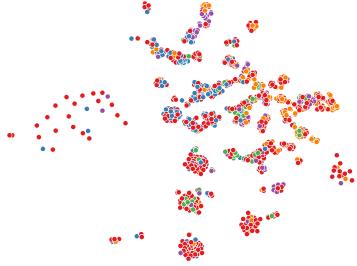
Table 10 suggests that using all seven classifiers is unnecessary. For example, on the Cora dataset, the combination of KNN, Random Forest, and Naive Bayes achieves the highest accuracy with minimal computational cost (only 3 seconds). This indicates that each of the seven classifiers has unique strengths suited to different tasks. However, selecting the optimal combination of base models remains an open area for theoretical analysis.
Accuracy and training time(s) on Cora dataset by combinations of different classifiers based on SStaGCN model. \topruleKNN Random Forest Naive Bayes Decision Tree GBDT Adaboost SVC Accuracy Training Time \colrule 91.2 13.90 93.6 16.60 84.2 567.9 92.9 144.7 93.1 149.5 92.8 15.90 93.4 18.80 92.9 568.3 92.9 570.7 92.8 708.5 \botrule
To further illustrate the impact of simplified stacking on the over-smoothing problem, we conduct an additional experiment on this topic. In Fig. 4(a), we observe that a conventional GCN tends to blend node features from different clusters as the number of convolutional layers increases. However, as shown in Fig. 5(a) and Table 11333The number of layers excludes those included in the stacking and aggregation parts of SStaGCN, which consist of only two layers., the proposed SStaGCN effectively mitigates the over-smoothing phenomenon and enhances accuracy.


Accuracy comparison between GCN and SStaGCN models on Cora dataset using distinct number of layers. \topruleMethod 2-layer 3-layer 4-layer 5-layer 6-layer 7-layer \colruleGCN 80.5 80.4 75.8 71.9 72.6 60.8 SStaGCN 93.3 88.8 87.5 86.4 84.8 84.3 \botrule
Overall, these experiments demonstrate the superiority of SStaGCN model over competitors.
4.5 Visualization


To further illustrate the performance of SStaGCN, we plot the final classification features of GCN, AdaGCN, BGNN, and our SStaGCN. Fig. 6(a) (for CiteSeer) and Fig. 7(a) (for DBLP) display the final classification features of each method on these datasets. As shown in these figures, the proposed SStaGCN misclassifies relatively fewer points, while GCN, AdaGCN, and BGNN result in more misclassified classes.
5 Conclusion
Traditional GCNs often face the over-smoothing problem. In this work, we propose a novel GCN architecture, SStaGCN, which leverages stacking and aggregation techniques to capture pre-classified data features, followed by GCN for predictions on distinct graph-structured data. SStaGCN effectively explores and utilizes features for heterogeneous graph data in a stacked manner. By incorporating classical machine learning methods, we design a GCN model that provides a versatile framework for handling diverse types of graph-structured data, offering new insights into understanding GCNs. Extensive experiments demonstrate that the proposed model outperforms several state-of-the-art competitors in terms of accuracy, F1-score, and training time. The framework presented here could also be extended to regression tasks. Additionally, we believe this method can address various types of heterogeneous graph data beyond tabular data. A promising future research direction is to investigate deeper GCNs within our framework, as suggested by [39]. The source code of SStaGCN will be issued soon 444https://github.com/dragon0916/SStaGCN..
Appendix
In this part, we provide a detailed proof of Theorem 3.1. Before proceeding with the proof, we introduce several supporting lemmas. First, we present the contraction inequality for Rademacher complexity in vector form.
Lemma 5.1.
[28] Let be any set, and be a class of functions ad let have Lipschitz constant . Then
where is an independent doubly indexed Rademacher sequence and is the th component of .
Lemma 5.2.
[2] Consider a loss function . Denote , and let be independently selected according to the probability measure . Then for any , with probability at least ,
We first give a lemma which plays essential role in the proof of Theorem 3.1.
Lemma 5.3.
Let for each node , then
Proof 5.4.
Denote as the sub-matrix of whose row and column indices belong to the set . Hence the size of depends on the node . Obviously, for . Let be the feature matrix of the nodes in (subgraph of ). Hence,
where is the th row of the matrix with column index belong to the set . Notice that
and . Therefore,
Now we are in position to give the proof of Theorem 3.1.
Proof 5.5 (Proof of Theorem 3.1).
To allow a slight abuse of notations, we will use to denote due to the explanation on page 3. Denote , with . Applying Proposition 4 in [13] to the case , we can attain the Lipschitz constant for standard softmax function is . Let stands for the th row of the matrix , for function set
the empirical Rademacher complexity is defined as
where is an i.i.d. family of Rademacher variables independent of . By the contraction property of Rademacher complexity,
and notice Lemma 5.2, we only need to bound . Therefore, we have the following estimate by utilizing Lemma 5.1.
where , notice the property of inner product, the above estimate can be further bounded as
the last inequality follows by the property that . Now the key point is how to estimate the term . We will employ the idea introduced in [26] (in the proof of Theorem 1) to remove the “sup” term. Let , , , with ,, and notice that , then we have
By the definition of Frobenius norm , the supremum of the above quantity under the constraint must be obtained when for some , and for all . Hence
Let be the th neighbor number of node (, ). Recall , with , therefore
Applying the conclusion and contraction property of Rademacher complexity again, we have
Therefore, we only need to estimate the term
Applying Cauchy-Schwartz inequality yields that
where the last inequality is due to the i.i.d condition of Rademacher sequences. Plugging the conclusion of Lemma 5.3 into the above term leads to
and
This completes the proof by combining with Lemma 5.2.
Acknowledgement
The work described in this paper was supported partially by the National Natural Science Foundation of China (12271111, 11871277), Special Support Plan for High-Level Talents of Guangdong Province (2019TQ05X571), Guangdong Basic and Applied Basic Research Foundation (2022A1515011726). The authors would like to thank Prof. Hong Chen from Huazhong Agricultural University for useful discussions about the theoretical analysis, which have helped to improve the presentation of the paper.
References
- [1] D. Bahdanau, K. Cho, and Y. Bengio, Neural machine translation by jointly learning to align and translate, in Int. Conf. on Learning Representations (ICLR), San Diego, United States (May 2015).
- [2] P. L. Bartlett and S. Mendelson, Rademacher and Gaussian complexities: risk bounds and structural results, in Int. Conf. on Computational Learning Theory & and European Conference on Computational Learning Theory, Amsterdam, Netherlands, (July 2001), pp. 224-240.
- [3] M. M. Bronstein, J. Bruna, Y. LeCun, A. Szlam, and P. Vandergheynst, Geometric deep learning: going beyond euclidean data, IEEE Sigal Proc. Mag. 34(4) (2017) 18-42.
- [4] J. Bruna, W. Zaremba, A. Szlam, and Y. Lecun, Spectral networks and locally connected networks on graphs, in Int. Conf. on Learning Representations (ICLR), Banff, Canada (April 2014).
- [5] S. Casas, C. Gulino, R. Liao, and R. Urtasun, Spagnn: spatially-aware graph neural networks for relational behavior forecasting from sensor data, in IEEE Int. Conf. on Robotics and Automation (ICRA), Paris, France (May 2020), pp. 9491-9497.
- [6] M. Chen, Z. Wei, Z. Huang, B. Ding, and Y. Li, Simple and deep graph convolutional networks, in Int. Conf. on Machine Learning (ICML), Virtual, (July 2020), pp. 1725-1735.
- [7] E. Chien, J. Peng, P. Li, and O. Milenkovic, Adaptive universal generalized pagerank graph neural network, in Int. Conf. on Learning Representations (ICLR), Virtual (May 2021).
- [8] M. Defferrard, X. Bresson, and P. Vandergheynst, Convolutional neural networks on graphs with fast localized spectral filtering, in Advances in Neural Information Processing Systems(NeurIPS), Barcelona, Spain (December 2016).
- [9] S. Dz̆eroski and B. Z̆enko, Is combining classifiers with stacking better than selecting the best one? Mach. Learn. 54 (2004) 255-273.
- [10] W. Feng, J. Zhang, Y. Dong, Y. Han, H. Luan, Q. Xu, Q. Yang, E. Kharlamov, and J. Tang, Graph random neural networks for semi-supervised learning on graphs, in Advances in Neural Information Processing Systems(NeurIPS), Virtual (December 2020), pp. 22092-22103.
- [11] Y. Freund and R. E. Schapire, A short introduction to boosting, Journal of Japanese Society for Artificial Intelligence 14 (1999) 771-780.
- [12] J. Friedman, Greedy function approximation: a gradient boosting machine, Ann. Stat. 29 (2001) 1189-1232.
- [13] B. Gao and L. Pavel, On the properties of the softmax function with application in game theory and reinforcement learning, Technical Report, arXiv:1704.00805 (2017).
- [14] M. Gori, G. Monfardini, and F. Scarselli, A new model for learning in graph domains, in Int. Joint Conf. on Neural Networks (IJCNN), Montreal, Canada (July 2005).
- [15] W. L. Hamilton, Z. Ying, and J. Leskovec, Inductive representation learning on large graphs, in Advances in Neural Information Processing Systems(NeurIPS), Long Beach, United States (December 2017).
- [16] D. K. Hammond, P. Vandergheynst, and R. Gribonval, Wavelets on graphs via spectral graph theory, Appl. Comput. Harmon. A., 30 (2011) 129-150.
- [17] S. Ivanov and L. Prokhorenkova, Boost then convolve: gradient boosting meets graph neural networks, in Int. Conf. on Learning Representations (ICLR), Virtual (May 2021).
- [18] D. Kingma and J. Ba, Adam: a method for stochastic optimization, in Int. Conf. on Learning Representations (ICLR), San Diego, United States (May 2015).
- [19] T. Kipf and M. Welling, Semi-supervised classification with graph convolutional networks, in Int. Conf. on Learning Representations (ICLR), Toulon, France (April 2017).
- [20] J. Klicpera, A. Bojchevski, and S. Günnemann, Predict then propagate: graph neural networks meet personalized pagerank, in Int. Conf. on Learning Representations (ICLR), New Orleans, United States (April 2019).
- [21] J. Klicpera, A. Bojchevski, and S. Günnemann, Predict then propagate: graph neural networks meet personalized pagerank, in Int. Conf. on Learning Representations (ICLR), New Orleans, United States (April 2019).
- [22] G. Li, M. Mueller, A. Thabet, and B. Ghanem, Deepgcns: can gcns go as deep as cnns? in Int. Conf. on Computer Vision (ICCV), Seoul, Korea (October 2019).
- [23] M. Li, Z. Ma, Y. G. Wang, and X. Zhuang, Fast haar transforms for graph neural networks, Neural Networks, 128(2020) 188-198.
- [24] Q. Li, Z. Han, and X. M. Wu, Deeper insights into graph convolutional networks for semi-supervised learning, in AAAI Conf. on Artificial Intelligence, New Orleans, United States (February 2018).
- [25] S. Luan, M. Zhao, X. W. Chang, and D. Precup, Break the ceiling: stronger multi-scale deep graph convolutional networks, in Advances in Neural Information Processing Systems(NeurIPS), Vancouver, Canada (December 2019).
- [26] S. Lv, Generalization bounds for graph convolutional neural networks via Rademacher complexity, Technical Report, arXiv:2102.10234 (2021).
- [27] L. V. D. Maaten and G. E. Hinton, Visualizing data using t-sne, J. Mach. Learn. Res. 9(2008) 2579-2605.
- [28] A. Maurer, A vector-contraction inequality for Rademacher complexities, in Int. Conf. on Algorithmic Learning Theory, Bari, Italy (October 2016).
- [29] V. Mnih, N. Heess, A. Graves, and K. Kavukcuoglu, Recurrent models of visual attention, in Advances in Neural Information Processing Systems(NeurIPS), Montreal, Canada (December 2014).
- [30] K. Pal and B. Patel, Data classification with k-fold cross validation and holdout accuracy estimation methods with 5 different machine learning techniques, in 2020 fourth Int. Conf. on Computing Methodologies and Communication (ICCMC), Erode, India (March 2020), pp. 83-87.
- [31] Y. Rong, W. Huang, T. Xu, and J. Huang, Dropedge: towards deep graph convolutional networks on node classification, in Int. Conf. on Learning Representations(ICLR), Virtual, (April 2020).
- [32] A. Sandryhaila and J. Moura, Discrete signal processing on graphs, IEEE Trans. Signal Processing 61(7) (2013) 1644-1656.
- [33] R. Schapire, Y. Freund, P. Barlett, and W. S. Lee, Boosting the margin: a new explanation for the effectiveness of voting methods, in Int. Conf. on Machine Learning (ICML), San Francisco, United States (July 1997).
- [34] F. Schwenker, Ensemble methods: foundations and algorithms, IEEE Comput. Intell. M. 8(2013) 77-79.
- [35] P. Sen, G. Namata, M. Bilgic, L. Getoor, B. Gallagher, and T. Eliassi-Rad, Collective classification in network data, AI Mag., 29(2008) 93-106.
- [36] D. I. Shuman, S. K. Narang, P. Frossard, A. Ortega, and P. Vandergheynst, The emerging field of signal processing on graphs: extending high-dimensional data analysis to networks and other irregular domains, IEEE Signal Proc. Mag. 30(3) (2013) 83-98.
- [37] J. M. Stokes, K. Yang, K. Swanson, W. Jin, and J. J. Collins, A deep learning approach to antibiotic discovery, Cell 180(4) (2020) 688-702.e13.
- [38] J. Sun, W. Guo, D. Zhang, Y. Zhang, F. Regol, Y. Hu, H. Guo, R. Tang, H. Yuan, X. He, and M. Coates, A framework for recommending accurate and diverse items using bayesian graph convolutional neural networks, in Proc. of the 26th ACM SIGKDD Int. Conf. on Knowledge Discovery & Data Mining, New York, United States (July 2020).
- [39] K. Sun, Z. Lin, and Z. Zhu, Adagcn: adaboosting graph convolutional networks into deep models, in Int. Conf. on Learning Representations (ICLR), Virtual (May 2021).
- [40] A. Vaswani, N. Shazeer, N. Parmar, J. Uszkoreit, L. Jones, A. N. Gomez, u. Kaiser, and I. Polosukhin, Attention is all you need, in Advances in Neural Information Processing Systems(NeurIPS), Long Beach, United States (December 2017), pp. 6000-6010.
- [41] P. Velickovic, G. Cucurull, A. Casanova, A. Romero, P. Lio’, and Y. Bengio, Graph attention networks, in Int. Conf. on Learning Representations (ICLR), Vancouver, Canada (April 2018).
- [42] X. Wang, H. Ji, C. Shi, B. Wang, Y. Ye, P. Cui, and P. S. Yu, Heterogeneous graph attention network, in The World Wide Web Conference, San Francisco, United States (May 2019 ), pp. 2022–2032.
- [43] D. Wolpert, Stacked generalization, Neural Netw. 5(1992) 241-259.
- [44] F. Wu, T. Zhang, A. Souza, C. Fifty, T. Yu, and K. Q. Weinberger, Simplifying graph convolutional networks, in Int. Conf. on Machine Learning(ICML), Long Beach, United States (June 2019).
- [45] B. Xu, H. Shen, Q. Cao, Y. Qiu, and X. Cheng, Graph wavelet neural network, in Int. Conf. on Learning Representations (ICLR), New Orleans, United States (May 2019).
- [46] L. Yao, C. Mao, and Y. Luo, Graph convolutional networks for text classification, in AAAI Conf. on Artificial Intelligence, Honolulu, USA (January 2019).
- [47] W. Yin, H. Schütze, B. Xiang, and B. Zhou, Abcnn: attention-based convolutional neural network for modeling sentence pairs, Transactions of the Association for Computational Linguistics, 4(2016) 259-272.
- [48] W. Zhang, Z. Sheng, Y. Jiang, Y. Xia, J. Gao, Z. Yang, and B. Cui, Evaluating deep graph neural networks, Technical Report, arXiv:2108.00955 (2021).
- [49] J. Zhu, Max-margin nonparametric latent feature models for link prediction, in Int. Conf. on Machine Learning (ICML), Edinburgh, UK (June 2012).