SSEGEP: Small SEGment Emphasized Performance evaluation metric for medical image segmentation

Ammu R\auno1 Neelam Sinha\auno2 ¹International Institute of Information Technology, Bangalore, India ²International Institute of Information Technology, Bangalore, India

Abstract

Automatic image segmentation is a critical component of medical image analysis, and hence quantifying segmentation performance is crucial. Challenges in medical image segmentation are mainly due to spatial variations of regions to be segmented and imbalance in distribution of classes. Commonly used metrics treat all detected pixels, indiscriminately. However, pixels in smaller segments must be treated differently from pixels in larger segments, as detection of smaller ones aid in early treatment of associated disease and are also easier to miss. To address this, we propose a novel evaluation metric for segmentation performance, emphasizing smaller segments, by assigning higher weightage to smaller segment pixels. Weighted false positives are also considered in deriving the new metric named, ”SSEGEP”(Small SEGment Emphasized Performance evaluation metric), (range : 0(Bad) to 1(Good)). The experiments were performed on diverse anatomies(eye,liver,pancreas and breast) from publicly available datasets to show applicability of the proposed metric across different imaging techniques. Mean opinion score (MOS) and statistical significance testing is used to quantify the relevance of proposed approach. Across 33 fundus images, where the largest exudate is 1.41%, and the smallest is 0.0002% of the image, the proposed metric is 30% closer to MOS, as compared to Dice Similarity Coefficient (DSC). Statistical significance testing resulted in promising p-value of order $10^{-18}$ with SSEGEP for hepatic tumor compared to DSC. The proposed metric is found to perform better for the images having multiple segments for a single label.

keywords:

Medical Image Segmentation \sepEvaluation Metric \sepSegmentation Evaluation \sepMultiple Segments \sepSmall Lesion Emphasized

1 Introduction

Medical images need to satisfy a certain diagnostic quality criteria in order to obtain reliable information from them. The array of available quality metrics has been studied by Allister et al. Paper6 , as applied to Magnetic Resonance (MR) images. Subsequently the images could be subjected to various processing, of which image segmentation is very important. The segmentation is done in different ways depending on the image modality and characteristics of the region to be segmented. Some common methods include histogram analysis, region segmentation, and edge detection. Universal Network (U-net) based deep learning methods are also widely used in medical image segmentation. The subsequent steps that follow segmentation include feature extraction and classification based on the considered task. Hence the quality of segmentation severely affects the proceeding stages and thereby arises the need of robust performance evaluation metrics.

General image segmentation and medical image segmentation: Evaluation of medical image segmentation should not be done similar to the general segmentation scenarios. State-of-the-art metrics include Accuracy, Sensitivity, Specificity, Dice Similarity Coefficient (DSC), Intersection Over Union (IOU) and boundary distance scores which are applicable to general segmentation scenarios. Information about overlap area between ground truth and segmented image is used to evaluate the quality of general image segmentation method. But medical image segmentation evaluation should also consider the diagnosis aspect, like what is more important in disease diagnosis. In certain cases, contour of the segment is of interest which requires the segmentation algorithm to provide exact boundary delimitation. But in other cases, location of the segment may be of interest. There may also be cases where the size/volume of the segment need to be analyzed. Some examples of medical segmentation scenarios include the detection and monitoring of tumor progress which is important in surgical planningp10 ; p11 ; p12 , change patterns in white matter that assists in early diagnosis and treatment of brain diseasesp13 . Other anatomic features in medical image segmentation include gray matter, lesions, organs and tumors. There are also medical scenarios where there are smaller segments that convey more information on disease grading/diagnosis.

Hence, the requirements on the segmentation algorithms for medical images depend on the goal of segmentation. Different evaluation metrics are sensitive to different properties of segmentations. Therefore, the evaluation metric should be chosen based on that. If only boundary of the region needs to be extracted, boundary-based distance scores can be used for evaluation. If it is required to know the total area/volume of a single tumor present in a tissue, DSC or IOU can be used for evaluation.

Segmentation challenges in medical images: The region to be segmented in medical images is not always distinct and localized. There may be regions with variation in location, size, shape and brightness. Preprocessing techniques usually take care of brightness and color. Other challenges include:

1.

Imbalance in data distribution: When the size of the segment is significantly smaller than the background, then the metrics based on calculation of True Negatives (TN) are not suitable. The number of TN pixels is always larger in medical images as shown in Figure 1. Accuracy,sensitivity, specificity and Positive Predictive Value (PPV) are not suitable for pixel level segmentation evaluation since the True Negative (TN) pixels which constitutes the major portion of the image is treated similar to that of other pixels. Pixel accuracy and specificity is usually high for medical images since TN is more. Quality of segmentation can’t be measured only with sensitivity as it does not consider the False Positives FPs. As PPV considers only the positive pixels, it can’t be used to asses the overall segmentation quality. So such classical metrics are not efficient for segmentation evaluation. DSC (Also known as F1-score) and IOU can be used in this case to overcome the above stated drawback as it considers the overlap between ground truth and prediction.

Figure 1: (a)Brain tumor CT slice(images taken from brainct , (b) Dynamic Contrast Enhanced (DCE-MRI) slice with color map and tumor mri_breastim , (c) Fundus images(image taken from DIARETDB1 dataset). In each of the image pairs, the image on the left is the original, while the image on the right is the segmentation ground truth hand marked by experts. The fraction of pixels in the ROI, in each of the cases, is very small. Number of TN pixels is large in all these cases compared to the TP pixels.
2.

Variation in size: Another challenge faced in medical segmentation is due to the size variation of the regions to be segmented. The region may appear clustered and not localized at a point. Here, the challenge of segmentation algorithm is to extract the tiniest segment. Smaller segments usually indicate the presence of associated disease at an earlier stage and hence it is required to emphasise these small sized segments more compared to larger ones. State-of-the-art metrics like sensitivity, specificity, DSC and IOU does not discriminate the segments based on the area. So it is imperative to design a metric that highlights the detection of smaller segments.

Figure 2: (a)Fundus image with exudates of various sizes circled in different colours. (b) Tumors in liver tissue of varying sizes.

Such a scenario can be seen in fundus images with exudates of various sizes as shown in Figure 2(a). A small protruding exudate may aid in early detection of diabetic retinopathy. Hepatic tumor is another example with multi-tumor case as seen in Figure 2(b). Another scenario is masses in mammograms which help to identify breast cancer.
3.

Multi-label segmentation with class imbalance: Multi-label segmentation arises when there are segments of different labels in a single image and class imbalance occurs when there is a relative size difference in segments of each class(label). For example, the image in Figure 3(a) consists of pancreas tissue and a tumor(which occupies a smaller space compared to pancreas) within that. The loss function of deep learning network(for segmentation) favours the large sized pancreas more than the tumor. But the loss function should be efficient to extract both the segments. Commonly used loss function for medical segmentation is Dice loss which is derived based on the evaluation metric DSC. But here, generalized Dice lossmultidice which works for multi label case should be used as it is not a simple binary segmentation. Another medical scenario is multi-label segmentation with more than one segment of various sizes in each category of label. Liver and tumor segmentation(Figure 3(b)) illustrates this situation with liver tissue and multiple hepatic tumors as the targets. In such a scenario, multi-label DSC is not sufficient to quantify the segmentation performance, as there may be segments of different sizes in each category of label and it is required to penalize the loss incurred by each pixel based on the area of the segment it belongs to.

Importance of small-sized segments in medical images Exudates are patches of fatty deposits on the eye formed due to leaky blood vessels. They appear as yellow-white structures in color fundus images with variable sizes, shapes and contrast. As exudates are among the common early clinical signs of Diabetic Retinopathy (DR), DR1 their detection would be critical in diagnosing the health status of the eye. The challenges faced in exudate segmentation include drastic variations in size(small to large as optic disc) and shape, and the severe imbalanced distribution of classes(more number of non-exudate pixels). The size of diabetic hard exudates changes with the progression of disease evidencefundus , hence the identification of tiny exudates is very important as it helps in the early treatment. So, the performance evaluation should be in such a way that it emphasizes the smaller exudates more. As the commonly used metrics treat all the TP pixels in similar way, they are not capable to quantify the small exudate segmentation. exudates1 have used sensitivity and PPV for exudate segmentation evaluation. exudates2 have used sensitivity, specificity, accuracy and area under curve of Receiver Operating Characteristic (ROC) as metrics to evaluate the detection of hard exudates using mean shift and normalized cut method.

Another medical segmentation scenario is in cancer detection. To detect cancer with Computer Aided Detection (CAD) techniques, tumor segmentation is inevitable. Tumors are visible in the Computed Tomography (CT) scans taken by the radiologist and it appears in various sizes. Pancreatic tumor is smaller in size compared to the large pancreatic tissue and a common algorithm for multi-label segmentation(pancreatic tissue and tumor) is a challenge faced in segmentation. The loss function used in training deep networks should overcome this imbalance due to size difference.

Refer to caption — Figure 3: (a) Multi-label segmentation: Pancreas(circled yellow) and tumor(circled black). (b) Multi-label segmentation with tumors of varying sizes. Tumors in (b) are shown enclosed in colored contours.

Most recent works use cross entropy and generalized DSCmultidice in this scenario. Numerous lesions of varying sizes may appear in a liver tissue called as hepatic lesions which can be malignant. Studies smallhepaticlesions have revealed the prevalence of small hepatic lesions found at CT in patients with cancer. These small lesions represent metastases in 11.6% patients as identified by the research study. The size of the lesions also changes during course of cancer and patients with small hepatic metastases also had associated extra hepatic metastases.

Calcifications are the earliest signs of breast cancer. Information about the size, density, and distribution of breast microcalcifications can give an idea about the benign or malignant nature of the cancer. It is found that decreasing calcifications is not a benign finding on mammogramdisapp_cal . Spontaneous decreases of calcifications are not necessarily indicative of better clinical outcomes. It has been demonstrated that a decrease in or complete resolution of breast calcifications is most concerning when it is associated with an extra breast mass, architectural distortion, or increased densitycalref1 ; calref2 . Small clusters of punctate or granular calcifications may represent high-grade DCIS(Ductal carcinoma in situ), where an aggressive clinical approach is recommendedcalref3 . If the calcifications are larger in size and well defined in shape, then it is less suspicious. But if they appear smaller in size or appear in varying shapes, then they are cancerouscalref4 . Hence, it is important to detect the smaller calcifications in mammograms.

The medical scenarios explained above states that the detection of smallest lesion is very critical in further medical analysis. The smallest exudate in Figure 2(a) occupies only 0.0002% of the image, the smallest tumor in Figure 3(a) and (b) occupies 0.0015% and 0.00004% of the respective images. A small protruding lesion may indicate the start of a disease. In most of the cases, one of the factors which is used to grade the disease severity is size/volume of the lesion or region of interest. As explained before, size of the hard exudates increase during the course of diabetic retinopathyevidencefundus , lesions become bigger with stages of cancer like hepatic cancer smallhepaticlesions and breast cancer. Hence, the detection of a tiny lesion helps in the early treatment of associated disease which can thereby avoid unnecessary biopsies. Also the detection of a small liver tumor may point the presence of a tumor in another regionsmallhepaticlesions . These studies enunciate that a performance evaluation metric that emphasizes these tiny lesions is imperative.

Olaf Ronneberger unet1 used UNet convolutional network for biomedical image segmentation. Keyvan Kasiri et al. keyvan used DSC to compare three brain MRI segmentation methods in software tools. A recent work reported by Ona et al. paper1 proposed an automated method to segment ischemic lesions in Diffusion-weighted MRI images using an ensemble of 3D convolutional neural networks (CNN). Dice score was utilized to evaluate the segmentation performance. The work reported by Piantadosi et al. paper2 achieves segmentation of breast parenchyma on volume MR data, utilizing an ensemble of CNNs. Dice score was utilized to quantify the segmentation accuracy. In the work reported by Ting et al. paper4 , the authors propose to improve segmentation accuracy by incorporating representation using Sparse Dictionary-based Learning, in the context of lesion segmentation in brain MR images. Nur et al. paper8 used saliency method based on region to detect exudates in retinal images of Diabetic Retinopathy. They have calculated accuracy, sensitivity and specificity for the evaluation of the proposed method. Abblin et al. paper9 calculated accuracy to evaluate the segmentation and recognition of iris from eye image. The authors used Fuzzy interference Logic based edge detection technique for segmentation. The work reported by Priya et al. paper10 used support vector neural network classifier for object and image level classification of Tuberculosis images and accuracy was calculated for evaluation. Fang Lu et al. paper11 used volumetric overlap error (VOE), relative volume diﬀerence (RVD), average symmetric surface distance (ASD), root mean square symmetric surface distance (RMSD) and maximum symmetric surface distance (MSD) to evaluate the deep learning algorithm with graph cut refinement to automatically segment liver in CT scans. Peter rot et al. paper12 reported work on deep sclera segmentation and recognition in which precision, recall and F1-score were used for segmentation evaluation and False Acceptance (FAR) and False Rejection error Rates (FRR) and Area Under the ROC curve (AUC) scores for the evaluation of recognition methods. An entirely different objective of comparing patch-based versus volumetric analysis of MR images was studied by Bontempi et al. Paper3 . Here, statistical significance testing was carried out to illustrate the superiority in segmentation performance while using entire volumes rather than patch-based analysis. The probability maps produced by the 2D and 3D-patch based methods are characterised by the presence of voxels associated with significant probability of belonging to the structure of interest (p ¿ 0.2) despite their distance from the latter. In the work reported by paper7 , the authors propose a method to segment structures in brain MR in Unsupervised setting, using Dice score and the Area under the Precision-Recall curve as the quantitative measures. dice1 ; dice2 also used DSC as an evaluation metric in medical image segmentation. multidice have used Generalized Dice overlap for segmentation assessment for unbalanced tasks. A reported work by Nabila et al. paper5 , discusses the issue of class imbalance in medical images. The authors propose generalized focal loss function in order to evaluate the segmentation performance on small-sized segments, using CNNs. However, in this approach, authors tweak the cost-function during the Training phase, in order to obtain better segmentation. familymetrics have introduced a family of metrics to quantify the difference or similarity of segments by considering their average overlap in fixed-size neighborhoods of points on the boundaries of those segments.

In order to quantify the segmentation performance of images with varying sizes of segments(exudates or tumors), we require a metric which emphasizes the smaller-sized segments. As seen before, DSC assigns the same weightage to all the TP pixels irrespective of whether it is part of large/small region, which seems inappropriate. The small segments should be penalized more while calculating the segmentation loss since the loss of few number of pixels in a small segment is severe than that in a large segment. The existing metrics as far as our knowledge, does not discriminate the detection of larger and smaller segment pixels. DSC and IOU metrics reflect the human understanding when the data set contains images with only large or only small segments with less false positives. For a clinical evaluation where screening has to be done, image level evaluation using sensitivity and specificity is enough. But to compare different segmentation methods or to optimize a single method, metrics that consider overlap between ground truth and segmented image is required. As the medical data sets usually consists of segments of varying sizes, evaluation with DSC and IOU is not sufficient as they treat all segments in the same way. The proposed metric which incorporates the area of segments and which penalizes the loss of smaller segments more would be more effective in comparing the segmentation approaches. This paper is organized as follows: section II discusses the commonly used evaluation metrics, section III presents the proposed approach in detail, section IV demonstrates the experimental results and analysis with the data sets used, followed by conclusion in section VI.

2 Existing Evaluation Metrics

Different evaluation metrics are used in practice to compare the effectiveness of various segmentation algorithms. The evaluation metric to be used depends on the problem and anatomy of the segmented region. To compare various medical segmentation methods, we need evaluation at pixel level for the entire image. The metric definitions of most popular evaluation methods are given in Table 2.

\tbl

Most popular evaluation metrics and their definitions are given. ’ $|$ $|$ ’ represents the cardinality. G and S constitutes the set of non-zero pixels in ground truth and prediction respectively. $|I|$ =TP+FP+FN+TN, ’ $l$ ’ is the label length in multi-label segmentation. \topruleMetric Formula \colruleAccuracy $\displaystyle Acc=\frac{|I|-|G\cup S|+|G\cap S|}{|I|}$ Sensitivity $\displaystyle Sens=\frac{|G\cap S|}{|G|}$ Specificity $\displaystyle Spec=\frac{|I|-|S\cup G|}{|I|-|G|}$ PPV $\displaystyle PPV=\frac{|G\cap S|}{|S|}$ IOU $\displaystyle IOU=\frac{|G\cap S|}{|G\cup S|}$ Hausdorff score $\displaystyle HD=$ (Boundary based score) $\displaystyle\max\{{\max_{x\epsilon\partial G}{d(x,\partial S)}},{\max_{y\epsilon\partial S}{d(y,\partial G)}}\}$ DSC $\displaystyle DSC=\frac{2|G\cap S|}{|S|+|G|}$ Generalized Dice score $\displaystyle GD=2\frac{\sum_{i=1}^{l}\frac{1}{|Gi|}|Gi\cap Si|}{\sum_{i=1}^{l}\frac{1}{|Gi|}(|Si|+|Gi|)}$ \botrule

An imbalance in data distribution is noticed in medical image segmentation where TN pixels is higher compared to other pixels, which makes classical metrics like accuracy and specificity inappropriate for performance evaluation.

Overlap metrics like DSC and IOU takes into account the area of overlap between the ground truth and segmented image. Both these metrics measure the same aspects and hence it is not required to use them together as evaluation metrics. Boundary distance based scores calculates the distance between the boundaries of segments in ground truth and prediction. They are used when boundary delineation of the segmentation is important. It does not take into account the size information of regions. Hausdorff Distance is not recommended to directly use in medical image segmentation as it is sensitive to outliersref_hau and time-consuming. Another interesting metric is MCC (Matthews Correlation Coefficient)mcc_ref which is symmetric in nature where no class is important than the other. It takes into account all four values in confusion matrix. It can be used when it is required to detect both the classes(when TN is also important) and/or classes are imbalanced.

If images in the data set consists of segments of various sizes, the segmentation algorithm should be able to detect most of the pixels in the smaller segment, even if it misses few larger segment pixels. So to assess the quality of prediction, the evaluation metric should be able to penalize more for smaller segment pixels than for larger segment pixels. This aspect is not considered in simple overlap and boundary distance based metrics. For the evaluation of multi-label segmentation performance as in pancreatic tumor, generalized Dice scoremultidice which gives a weightage of inverse of total area for each label is used. But if there are many segments in a single class(many hepatic lesions), DSC is not sufficient for performance evaluation as it can’t discriminate between the segments in a single class. Few synthetic images which represent different binary segmentation scenarios are constructed as shown in Figure 4. The distance between the boundaries of ground truth and prediction for the images in (b) and (c) are same even though two different cases are depicted, which shows the failure of boundary based metric. Since same number of pixels are lost in (e) and (f), DSC will be the same for both, even though a full small segment is lost as seen in (f). This drawback is overcome by the proposed metric as it weighs the TP pixels based on the area of the segment it is derived from. Higher weightage is given to the smaller segment pixels and lower weightage to the larger segment pixels.

3 Methodology

3.1 Proposed Metric

We have proposed an evaluation metric to quantify the performance of various segmentation scenarios, especially the cases where small segments in the prediction need to be emphasized more. We have illustrated the analysis in medical scan images which contains segments of various sizes. The proposed metric, SSEGEP penalizes the loss of smaller segments more in comparison to the larger ones. Each pixel in the ground truth image is assigned a weightage which is calculated based on the area of the segment it belongs to. Weightage of a segment is the inverse of its area, which results in high-weighted small sized segments and low-weighted bigger segments. So while calculating SSEGEP, instead of simple count of true positive pixels, weighted sum of TPs (True Positive) is considered. FP pixels are also weighted which is given as the inverse of TP count. If the task given is to quantify the combined segmentation of organ and tumor, two different weights are given to the FP pixels: one for tumor case, which is given as the inverse of TP count of tumor mask and other for organ case, which is given as the inverse of TP count of organ mask.

3.2 Implementation and Explanation

The general block diagram for 2D images is shown in Figure 5. The ground truth and segmented images are given as inputs. Segments of label 1 and 2 are given in different colors. The segmentation evaluation methodology is comprised of assigning weightage to segments in ground truth image, finding true positive pixels in each segment, finding and assigning weightage to the false positive segments and final calculation of proposed metric. Initially, from the ground truth image, distinct segments belonging to each label is found. Here, in the block diagram, there are two different labels and every distinct segment of these two labels are found. Similarly, the distinct segments of each label are found from the segmented image. This is done by finding the contours of the input image. Then, a weightage is allotted to these ground truth segments which is given as the inverse of area of that segment as shown in Figure 5. Then, the count of pixels in TP segments(overlapping region of segments between ground truth and prediction) is calculated which is given by $a_{i}$ as shown in the block diagram. XOR operation is performed separately for each label between the groundtruth and segmented image to find the false positive images for each label(Here, two FP images are obtained as there are two labels), and the separate count of these pixels is recorded. Weightage of inverse TP count is given to those FP pixels as shown in the block diagram. So, when the count of FP is very much higher than that of TP, SSEGEP value becomes small indicating poor segmentation, and when the count of FP is small compared to TP, SSEGEP value becomes high indicating good segmentation(provided FN is less). Final SSEGEP value is calculated from these set of metrics which quantifies the quality of the prediction. The proposed metric is given by equation (1).

\textit{SSEGEP}=\frac{\sum_{i=1}^{n_{s}}{w_{tpi}}{a_{i}}}{n_{s}+\sum_{j}{n_{fpj}}}

(1)

Where $w_{tpi}$ and $a_{i}$ represents the weightage and TP count of $i^{th}$ segment respectively and $n_{s}$ represents the total number of segments in the ground truth image. Here, $i$ is used to indicate segment and $j$ to indicate label.

n_{fpj}=fpj*(\frac{1}{\sum_{label(a_{i})=j}{a_{i}}})

(2)

Where $fp_{j}$ represents the total FP count for segments of label j.

4 Experimental Details and Materials Used

The experiments are performed on synthetic images to illustrate the proof of concept and real scan images of three different modalities: Fundus, mammogram and CT to analyse and compare the proposed metric in different scenarios with other state-of-the-art metrics. Segmentation evaluation was done on:

(a) Images with multiple segments from same class: The images may contain segments of various sizes in which smaller segment is crucial in disease diagnosis. For eg, liver contain multiple tumors, fundus image consists of exudates and mammograms with calcifications of various sizes.

(b) Images with multiple segments from two different classes: Usually a single algorithm may not be efficient to extract segments of different labels in multi-label segmentation. In scenarios where a common algorithm is required to perform multi-label segmentation where the smaller segments are more important in disease diagnosis, it is imperative to use an evaluation metric which discriminates the segments in such a way weighting smaller segments more. As the proposed metric SSEGEP assigns size-based weight to the segments in the input image, smallest segment gets the highest importance and the larger one gets the least weightage.

Further, the relevance of proposed metric, SSEGEP is analysed with two different approaches:

(1) Mean opinion score: The proposed metric is compared with TPR and Dice score and its relevance is tested with mean opinion score calculated based on the scores assigned by 15 subjects on the 33 fundus segmentation results obtained. The scores were given in the range of (0,0.25,0.5,0.75,1) where 0 and 1 indicating poor and best segmentation respectively. Then the average of the difference between mean opinion score and value of the evaluation metric is found which indicates the deviation of that metric from the mean opinion score.

(2) Hypothesis testing: As we have a greater number of images in liver, pancreas and mammogram data sets, statistical significance of SSEGEP was measured separately for each data set by hypothesis testing. To assess the statistical significance of the proposed metric for mammogram database, Welch’s t-test was performed since Levene’s test for homogeneity of variances indicated unequal variances between groups and sample sizes were unequal. Two tests were performed for a single data set: one for Dice value and other for SSEGEP. The inputs for the test are metric values for very good and very poor segmentation(extreme cases are considered for better understanding).The threshold to TP and FP to decide the samples in two groups were selected as: If TPR is greater than 80% and FPR and FNR are lesser than 20%, then the corresponding segmented image belongs to ’good segmentation’ category. If TPR is less than 40% and FPR and FNR are more than 50%, then the image belongs to ’bad segmentation’ category. To conduct the test for SSEGEP, the SSEGEP values for ’good segmentation’ category forms one input and the SSEGEP values for ’poor segmentation’ category forms the other input. Significance level ( $\alpha$ ) is set to be 0.00001. If the resulting p-value is lesser than the set significance level, then the data is said to be statistically significant, which means that two populations have unequal means. The same test is repeated for Dice to obtain the p-value.

All metric values Dice, Accuracy, IOU and SSEGEP – lie in the range 0 to 1 Python 3.6 is used for the implementation.

4.1 Datasets Used

We have used four different publicly available data sets to evaluate the significance of our metric. They are-

1.

DIARETDB1 - containing fundus images (Imaging modality = Fundus, anatomy = eye)
2.

CBIS-DDSM - containing mammogram images (Imaging modality = Mammogram, anatomy = breast)
3.

MSD challenge - containing liver images (Imaging modality = CT, anatomy = liver)
4.

MSD challenge - containing pancreas images (Imaging modality = CT, anatomy = pancreas)

They are all publicly available databases, with 89 images of the eye, 131 training images of the liver, 282 training images of pancreas, 173 training images of the breast with calcification upon which several research groups have evaluated their algorithms. Overall, 379 images from real scans, were used to illustrate the performance of the proposed metric.

DIARETDB1misc1 database is considered which consists of fundus images with exudates of various sizes. This is a publicly available database comprising of 89 fundus images in which 48 contains signs of hard exudates as marked by the experts. As exudates are early signs of Diabetic Retinopathy, good segmentation algorithms which can segment even the very smallest exudate is required. It is also required to evaluate the segmentation approach by a metric which emphasizes the tiniest exudates. Here, we have obtained the segmented images using the multi-space clustering approach given by inbook1 . 15 images with varying sizes of exudates were hand-chosen for training and 33 random images for testing. Original images are of size 1500 pixels x 1152 pixels, and were down-sized to 800 pixels x 615 pixels, to enable the running of the segmentation algorithm. The largest exudate present is 1.41%,and the smallest is 0.0002% of the image. Few sample images in the database with exudates are shown in Figure. 6.

CBIS-DDSM database is considered which is a standardized version of DDSM database. The mammogram images are in DICOM format. U-net based segmentation approachunet1 is used to obtain the segmentation results for calcifications. 108 images were considered for the evaluation of the proposed metric. The images were cropped to remove the majority black pixels in the background for U-net segmentation. First column in Figure 10 shows sample mammogram images with calcifications.

131 abdomen images with various number of slices are taken from Medical Segmentation Decathlon challenge train data set (source: IRCAD Hôpitaux Universitaires)DBLP:journals/corr/abs-1902-09063 of Portal venous phase CT modality with liver and tumor as targets for segmentation. The data set is rich in terms of the challenges and variability of the images contained in it. The ground truth images in this data set is multi-labeled, where 0,1, and 2 are the respective labels for background, liver and tumor. The segmented images are obtained using the nnU-Net framework proposed by DBLP:journals/corr/abs-1904-08128 . Few sample slices with tumors are shown in Figure 7. Tumor appears in various sizes as seen in the figure.

107 abdomen images with various number of slices are taken from MSD challenge train data set (source: Memorial Sloan Kettering Cancer Center)DBLP:journals/corr/abs-1902-09063 of Portal venous phase CT modality with segmentation targets as pancreas and tumor. The data set contains cases with good variability. The segmented images are obtained using the nnU-Net framework proposed by DBLP:journals/corr/abs-1904-08128 . Here, only one tumor is present in a pancreas segment. In some slices, the pancreas tissue and tumor are of similar size, whereas in few slices, tumor is very small compared to the tissue leading to class imbalance.

5 Results and Discussion

The effectiveness of our metric in the evaluation of segmentation performance is demonstrated in this section. Results obtained on applying the proposed metric on each of the datasets has been has been reported. Comparisons with the existing widely-used metrics has also been presented. Besides, Hypothesis testing in order to establish the statistical significance of the proposed metric is also carried out.

5.1 Experiments with synthetic images

Few synthetic images with multiple segments of varying sizes which represent different segmentation scenarios are constructed as shown in Figure 8. The values of state-of-the-art metrics wrongly indicate that the result of second segmentation( 8(c)) is better than that of third segmentation(8(d))(It is because the number of detected exudate pixels with second algorithm is greater than that of third algorithm). But a small exudate is missed in 8(c), which means the corresponding segmentation algorithm is not efficient in detecting smaller exudates. The proposed metric can discriminate these cases as it weighs the TP pixels based on the area of the segment it is derived from. SSEGEP for 8(d) is higher than 8(c) which indicates that quality of prediction is better with algorithm 3 than algorithm 2.

5.2 Experiments with real scan images

5.2.1 Experiments with retina images-Multiple segments of same type

Figure 9 shows few fundus images with their ground truth and segmentation. The values of proposed metric and commonly used state-of-the-art metrics are compared with the average Mean Opinion Score. True positive rate is not sufficient to evaluate segmentation performance as it does not take into account the false positives(High TPR in row 2 which is a poor segmentation). Dice value can be used when there is no much variation in exudate size(rows 1,2,5). But Dice fails to quantify segmentation performance when there are exudates of varying sizes(row 4). In such a case, SSEGEP outperform other metrics as it is capable to discriminate different segments according to the count of the pixels in it.

\tbl

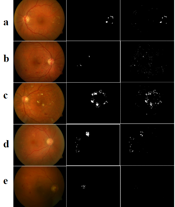
A comparison of commonly used evaluation metrics with the proposed metric for fundus images in Figure 9 with exudates. Mean Opinion Score(MOS) is given in the last row. \toprulePanel Sensitivity Acc Dice IOU SSEGEP MOS \colrulea 0.66 0.73 0.68 0.52 0.63 0.75 b 0.63 0.57 0.22 0.12 0.20 0.20 c 0.63 0.37 0.68 0.51 0.75 0.76 d 0.39 0.51 0.53 0.36 0.82 0.81 e 0.02 0.80 0.04 0.02 0 0.03 \botrule

The average of the difference between mean opinion score and value of the evaluation metric(SSEGEP,Dice and Sensitivity) are tabulated in Table 5.2.1. The deviation value is least with the proposed metric which indicates its higher correlation with human interpretability.

\tbl

Comparison of proposed metric with the state of the art metrics on the DIARETDB1 database is shown in second column.Average deviation of few evaluation metrics from the mean opinion score evaluated by 15 subjects is given in column 3. Comparison is done on a scale of 0 to 1. \topruleEvaluation Average Value Average deviation Metric obtained(Pixel level) wrt to MOS \colruleSensitivity 0.4003 0.12 Dice value 0.3539 0.11 SSEGEP(proposed) 0.3324 0.08 \botrule

5.2.2 Experiments with mammogram images-Multiple segments of same type

Figure 10 shows sample fundus images with their ground truth and segmentation masks. Table 5.2.2 shows the values of proposed metric and other commonly used metrics. Here, comparison is also made with another evaluation metric, MCC(Matthews correlation coefficient). As seen in the fundus images, sensitivity and accuracy are not sufficient to quantify the segmentation performance. Panels ’a’ to ’e’ consists of calcifications of varying sizes. Smaller calcifications indicate the higher severity of disease. Even though smaller segment is lost in mammogram segmentation for those panels, state-of-the-art metrics fail to reflect it. For eg., the Dice value is 0.91 for mammogram in panel ’a’ even though the segmentation algorithm failed to detect the smaller segment. But, SSEGEP is 0.43 which indicates the poor segmentation in terms of medical diagnosis. Panels ’f’ and ’g’ consists of calcifications of similar sizes, hence the values of proposed metric, SSEGEP is comparable to state-of-the-art metrics. Panel ’h’ comprises of a single large segment, and hence all metric values are of similar range.

\tbl

A comparison of commonly used evaluation metrics with the proposed metric for mammogram images in Figure 10 with calcification. \toprulePanel Sensitivity Acc Dice IOU MCC SSEGEP \colrulea 0.84 0.96 0.91 0.84 0.88 0.43 b 0.59 0.95 0.68 0.52 0.66 0.39 c 0.78 0.95 0.76 0.61 0.73 0.59 d 0.35 0.99 0.49 0.32 0.53 0.29 e 0.70 0.97 0.81 0.68 0.81 0.40 f 0.83 0.98 0.89 0.81 0.89 0.81 g 0.48 0.99 0.54 0.37 0.54 0.42 h 0.89 0.94 0.94 0.88 0.89 0.88 \botrule

The bar plots of SSEGEP values and Dice values for few samples of images are shown in Figure 11. Dice and SSEGEP values for images of good segmentation category are almost in the same range. It implies that both the metrics are able to reflect good segmentations. But the Dice values for many images under poor segmentation category are higher than that of SSEGEP values. Even though the segmentation result is poor, Dice values are high. But the proposed metric is able to reflect the poor quality of segmentation, since those values are lower.

The results for statistical significance test are tabulated in Table 5.3. The p-value for SSEGEP is lesser than that of Dice value, which indicates the better discriminating capability for the proposed metric.

5.2.3 Experiments with Liver images

Multiple segments(tumors) of same type

Figure 12,13 and 14 shows the evaluation metrics obtained for few sample cases of (1) images with all small tumors, (2) images with small and large tumors and (3) images with similar sized(medium sized) tumors. Here, performance evaluation is conducted only for tumors. Accuracy for all the cases is high(0.98,0.99) as the number of TN pixels is high compared to other pixels. As seen in Figure 12, all the tumors appear small. SSEGEP and IOU values are varying in a similar way. Dice values are slightly higher than IOU as the former gives higher weightage to TP pixels. Since the tumors are smaller in size, even though few pixels are missed in segmentation, it should be highly penalized which is reflected by the proposed metric.

Figure 13 consists of tumors of varying sizes. There are tiny tumors and large tumors present in a single tissue. So, the loss of a small tumor should be highly penalized. But still the values of other metrics are closer to 0.90. However, SSEGEP value is in the range of 0.70-0.75, thereby reflecting the level of quality of segmentation.

Figure 14 comprises of scan images with similar and moderately sized tumors. The SSEGEP values are comparable with other commonly used metrics because of similar sized segments. There is a FP present in the third case which resulted in lesser SSEGEP value compared to other two cases. Since weightage of FP is decided by the inverse of TP pixels and number of TP pixels is less in this case, SSEGEP value is not too low.

Hence, we can conclude that if there are tumors of varying sizes in ground truth and if the segmentation algorithm fails to extract the smaller tumors, it should be severely penalized (as seen in Figure 13). As it can be clearly seen in Figure 13, even though other metric values are at a higher side indicating best segmentation, proposed metric is lesser than that since smaller tumors are lost in segmentation. Commonly used metrics fails to discriminate the varying sized distinct tumors. But the proposed metric assigns different weightage to tumors based on their size, emphasizing smaller ones.

Multi-label case with many segments of different types(liver and tumor)with class imbalance

Figure 15 shows sample multi-label segmentation and the corresponding evaluation metrics. Here, SSEGEP is compared with the generalized multi class Dice value which is the commonly used performance metric for unbalanced multi-class segmentation. Even though generalized multi class Dice can discriminate the two different labels, it fails to differentiate the multi-sized tumors present. As seen in the figure 15, liver occupies more space compared to the tumors. Even though small tumors are not identified in each case, Dice value is same as it gives the same weightage to every tumor irrespective of their size. But SSEGEP value is not high unlike Dice value since the proposed metric emphasizes the smallest tumor more by assigning a higher weightage to it, thereby penalizing the loss of smaller segments.

The results for hypothesis testing are tabulated in Table 5.3. The test says that the inputs come from different distributions for both the metrics with p-value for SSEGEP lesser than that of Dice value. This implies that both the metrics(SSEGEP and Dice) are able to distinguish between good and poor segmentation, with a better discriminating capability for SSEGEP.

5.2.4 Experiments with pancreas images-Multi-label case with one segment each of different type(pancreas and tumor)

Here, only one tumor is present in a pancreas segment. So, the evaluation is done for combined pancreas and tumor image as explained for liver and tumor case. Sample images with generalized multi class Dice and SSEGEP values are shown in Figure 16. Tumor is not detected for ground truth in the first and last column in Figure 16. For all cases, Dice and SSEGEP values vary in similar way, since each class(pancreas and tumor) contains only one segment(one tissue and one tumor) unlike combined liver and tumor case(in liver and tumor segmentation, there were multiple tumors in the liver tissue). Hence, for multi label segmentation evaluation where there is only one segment present in a class(or label), either generalized Dice or SSEGEP can be used.

The results for hypothesis testing are tabulated in Table 5.3. The p-value is same for both metrics, indicating the applicability of both metrics in that case. This is because there is only one segment corresponding to each label in an image slice and both SSEGEP and generalized Dice acts in similar way for that scenario, whereas in liver tumor segmentation there are tumors of various sizes and the size variation within a label is not reflected by Dice value.

5.3 Analysis of impact of parameter changes on SSEGEP

The various parameters used in the study are:

1.

Number of connected components in the Ground Truth: If the number of connected components in the Ground Truth, as an extreme case, happens to be only 1, then the proposed metric would not result in any significantly different way compared to Dice score, since it simply involves the calculation of total overlap area like Dice score.
2.

The Relative sizes of each of the connected components in the Ground Truth: If the sizes of each of the connected components in the Ground Truth are all comparable, then the advantage of assigning them different weights will not lead to much distinction across them. However, if the sizes of the connected components in the Ground Truth are very diverse, then the significance of assigning differential weights to each of them becomes very perceptible.
3.

Updated Weightage for TP: Weightage assigned to TP depends on the size of the corresponding connected component in groundtruth. If the connected component is of smaller size, higher weightage is assigned to that TP pixel, and vice-versa.
4.

Updated Weightage for FP: Weightage assigned to FP depends on the size of total TP pixels. When the number of FP pixels is less, the segmentation performance is better and when FP is more, segmentation performance is poor. To weight the FP pixels, inverse of TP pixels is considered. Hence if the FP count is higher than TP count, a higher weightage is assigned to FP thereby leading to smaller value of SSEGEP.

\tbl

Hypothesis Testing with $\alpha=0.00001$ . \topruleSegmentation scenarios p value(Dice) p value(SSEGEP) \colruleCalcification 1.8e-19 3.5e-35 Tumor(liver) 7.6e-12 1.2e-18 Combined liver-tumor 2.9e-17 3.6e-19 Combined pancreas-tumor 3.3e-19 3.3e-19 \botrule

Limitations of proposed metric

The above experiments say that proposed metric gives a better performance than other metrics for the evaluation of segmentation performance of medical images with segments of varying sizes. For images with segments of similar size, SSEGEP performs in similar way as other overlap based metrics(Dice score,IOU). If the segmentation is done in random or by chance, the metric value should ideally be zero. But this is not the case with SSEGEP.

6 Conclusion

The segmentation of smaller lesions that appear in medical image scans are important as they assist in the early treatment of associated diseases. The evaluation metric used should be able to quantify the segmentation performance emphasizing these smaller lesions. The proposed metric assigns weightage to each segment in the image based on their area in such a way to emphasize the smaller segments more. The applicability of our metric across different imaging techniques is shown by testing in four public datasets of different anatomies and its significance is proved with mean opinion score and hypothesis testing. It is observed that the proposed metric is 30% closer to MOS, as compared to DSC for fundus images and statistical significance testing resulted in promising p-value of the order $10^{-18}$ with SSEGEP for liver tumor compared to Dice Similarity Coefficient. The experimental results show that the proposed metric outperforms other metrics with respect to human interpretability and understanding for those images with multiple segments of various sizes.

Acknowledgements

We would like to thank Fabian Isensee for providing the segmentation results of pancreas and liver images that are obtained using nnU-Net DBLP:journals/corr/abs-1904-08128 . We also acknowledge Sanjeev Dubey for providing detailed analysis in GitHub about the segmentation algorithm inbook1 used for fundus images.

References

[1] A. Mason, J. Rioux, S. E. Clarke, A. Costa, M. Schmidt, V. Keough, T. Huynh, and S. Beyea. Comparison of objective image quality metrics to expert radiologists’ scoring of diagnostic quality of mr images. IEEE Transactions on Medical Imaging, pages 1–1, 2019.
[2] Kelly Zou, Simon Warfield, Aditya Bharatha, Clare Tempany, Michael Kaus, Steven Haker, William Wells, Ferenc Jolesz, and Ron Kikinis. Statistical validation of image segmentation quality based on a spatial overlap index. Academic radiology, 11:178–89, 2004.
[3] KH Zou, WM Wells, R Kikinis, and SK Warfield. Three validation metrics for automated probabilistic image segmentation of brain tumours. Stat Med, 23:1259–82, 2004.
[4] Andrew Worth, Makris Nikos, Verne Caviness, and David Kennedy. Neuroanatomical segmentation in mri: Technological objectives. International Journal of Pattern Recognition and Artificial Intelligence, 11:1161–87, 11 1997.
[5] SK Warfield, CF Westin, CRG Guttmann, MS Albert, FA Jolesz, and R Kikinis. Fractional segmentation of white matter. In International Conference on Energy Efficient Technologies for Sustainability (ICEETS), pages 109–117, 1999.
[6] A. Nanthagopal and R Sukanesh. Combined texture feature analysis of segmentation and classification of benign and malignant tumor ct slices. Journal of medical engineering & technology, 37, 10 2012.
[7] Mohammed El Adoui, Sidi Mahmoudi, Amine Larhmam, and Mohammed Benjelloun. Mri breast tumor segmentation using different encoder and decoder cnn architectures. Journal of Computers, 8:52, 06 2019.
[8] Carole Sudre, Wenqi Li, Tom Vercauteren, Sebastien Ourselin, and Manuel Jorge Cardoso. Generalised dice overlap as a deep learning loss function for highly unbalanced segmentations. In Deep Learning in Medical Image Analysis and Multimodal Learning for Clinical Decision Support, pages 240–248, 09 2017.
[9] R Klein, B.E.K. Klein, S E Moss, M D Davis, and David Demets. The wisconsin epidemiologic study of diabetic retinopathy. vii. diabetic nonproliferative retinal lesions. Ophthalmology, 94:1389–400, 12 1987.
[10] Prisca Loganadane, Bernard Delbosc, and Maher Saleh. Short-term progression of diabetic hard exudates monitored with high-resolution camera. Ophthalmic Research, pages 1–7, 11 2018.
[11] Qing Liu, Beiji Zou, Jie Chen, Wei Ke, Kejuan Yue, Zailiang Chen, and Guoying Zhao. A location-to-segmentation strategy for automatic exudate segmentation in colour retinal fundus images. Computerized Medical Imaging and Graphics, 55, 09 2016.
[12] Sreeparna Banerjee and Diptoneel Kayal. Detection of hard exudates using mean shift and normalized cut method. Biocybernetics and Biomedical Engineering, 36, 10 2016.
[13] Lawrence Schwartz, Eric Gandras, Sandra Colangelo, Matthew Ercolani, and David Panicek. Prevalence and importance of small hepatic lesions found at ct in patients with cancer. Radiology, 210:71–4, 02 1999.
[14] Quan Nguyen, Nga Nguyen, Linden Dixon, Flavia Monetto, and Angelica Robinson. Spontaneously disappearing calcifications in the breast: A rare instance where a decrease in size on mammogram is not good. Cureus, 12, 06 2020.
[15] Benoit Mesurolle, Fawaz Halwani, Vincent Pelsser, Jean Gagnon, Ellen Kao, and Francine Tremblay. Spontaneous resolving breast microcalcifications associated with breast carcinoma. The breast journal, 11:478–9, 11 2005.
[16] H. Seymour, J. Cooke, and R. Given-Wilson. The significance of spontaneous resolution of breast calcification. The British journal of radiology, 72 853:3–8, 1999.
[17] A Evans, K Clements, A Maxwell, H Bishop, A Hanby, G Lawrence, et al. Lesion size is a major determinant of the mammographic features of ductal carcinoma in situ: findings from the sloane project. Breast Cancer Research, 65:181–4, 2010.
[18] Breastcancer.org. Understanding Breast Calcifications, 2018 (accessed October 13, 2020).
[19] Olaf Ronneberger, Philipp Fischer, and Thomas Brox. U-net: Convolutional networks for biomedical image segmentation, 2015.
[20] Keyvan Kasiri, Mohammad Dehghani, Kamran Kazemi, Mohammad Helfroush, and S Kafshgari. Comparison evaluation of three brain mri segmentation methods in software tools. In 2010 17th Iranian Conference of Biomedical Engineering (ICBME), pages 1 – 4, 12 2010.
[21] Ona Wu, Stefan Winzeck, Anne-Katrin Giese, Brandon Hancock, Mark Etherton, Mark Bouts, Kathleen Donahue, Markus Schirmer, Robert Irie, Steven Mocking, Elissa McIntosh, Raquel Bezerra, Konstantinos Kamnitsas, Petrea Frid, Johan Wasselius, John Cole, Huichun Xu, Lukas Holmegaard, Jordi Jimenez-Conde, and Natalia Rost. Big data approaches to phenotyping acute ischemic stroke using automated lesion segmentation of multi-center magnetic resonance imaging data. Stroke, 50, 06 2019.
[22] Gabriele Piantadosi, Mario Sansone, Roberta Fusco, and Carlo Sansone. Multi-planar 3d breast segmentation in mri via deep convolutional neural networks. Artificial Intelligence in Medicine, page 101781, 12 2019.
[23] Ge, Mu Ting, Zhan Ning, Chen Tianming, Gao Zhi, Mu Wanrong, and Shanxiang. Multi-planar 3d breast segmentation in mri via deep convolutional neural networks. Computational intelligence and neuroscience, 7 2019.
[24] N Nur and Handayani Tjandrasa. Exudate segmentation in retinal images of diabetic retinopathy using saliency method based on region. Journal of Physics: Conference Series, 1108:012110, 11 2018.
[25] A R Abblin and S A Praylin Selva Blessy. Automatic segmentation and recognition of iris from an eye image. In International Conference on Energy Efficient Technologies for Sustainability (ICEETS), 2018.
[26] Ebenezer Priya and S. Srinivasan. Automated object and image level classification of tb images using support vector neural network classifier. Biocybernetics and Biomedical Engineering, 36, 07 2016.
[27] Fang Lu, Fa Wu, Peijun Hu, Zhiyi Peng, and Dexing Kong. Automatic 3d liver location and segmentation via convolutional neural network and graph cut. International Journal of Computer Assisted Radiology and Surgery, 12, 09 2016.
[28] Peter Rot, Matej Vitek, Klemen Grm, Žiga Emeršič, Peter Peer, and Vitomir Štruc. Deep Sclera Segmentation and Recognition, pages 395–432. Springer International Publishing, Cham, 2020.
[29] Dennis Bontempi, Sergio Benini, Alberto Signoroni, Michele Svanera, and Lars Muckli. Cerebrum: a fast and fully-volumetric convolutional encoder-decoder for weakly-supervised segmentation of brain structures from out-of-the-scanner mri. ArXiv, abs/1909.05085, 2019.
[30] Christoph Baur, Benedikt Wiestler, Shadi Albarqouni, and Nassir Navab. Fusing unsupervised and supervised deep learning for white matter lesion segmentation. In International Conference on Medical Imaging with Deep Learning – Full Paper Track, London, United Kingdom, 08–10 Jul 2019.
[31] Piotr Chudzik, Somshubra Majumdar, Francesco Caliva, Bashir Al-Diri, and Andrew Hunter. Exudate segmentation using fully convolutional neural networks and inception modules. In Medical Imaging 2018: Image Processing, volume 10574, pages 785 – 792. SPIE, 2018.
[32] Sylvain Gouttard, Martin Styner, Marcel Prastawa, Joseph Piven, and Guido Gerig. Assessment of reliability of multi-site neuroimaging via traveling phantom study. In Dimitris Metaxas, Leon Axel, Gabor Fichtinger, and Gábor Székely, editors, Medical Image Computing and Computer-Assisted Intervention – MICCAI 2008, pages 263–270, Berlin, Heidelberg, 2008. Springer Berlin Heidelberg.
[33] Abraham Nabila and Khan Naimul. A novel focal tversky loss function with improved attention u-net for lesion segmentation. In 2019 IEEE International Symposium on Biomedical Imaging (ISBI), 2019.
[34] Varduhi Yeghiazaryan and Irina Voiculescu. Family of boundary overlap metrics for the evaluation of medical image segmentation. Journal of Medical Imaging, 5:1, 02 2018.
[35] Abdel Aziz Taha and Allan Hanbury. Metrics for evaluating 3d medical image segmentation: analysis, selection, and tool. BMC medical imaging, 15:29, 2015.
[36] Pierre Baldi, SÃ¸ren Brunak, Yves Chauvin, Claus Andersen, and Henrik Nielsen. Assessing the accuracy of prediction algorithms for classification: An overview. Bioinformatics (Oxford, England), 16:412–24, 06 2000.
[37] V. Kalesnykiene, J. k. Kamarainen, R. Voutilainen, J. Pietilä, H. Kälviäinen, and H. Uusitalo. Diaretdb1 diabetic retinopathy database and evaluation protocol, 2007.
[38] Sanjeev Dubey and Utkarsh Mittal. Exudate detection in fundus images: Multispace clustering approach. In Third International Conference, ICICCT 2018, pages 109–117, 01 2019.
[39] Amber L. Simpson, Michela Antonelli, Spyridon Bakas, Michel Bilello, Keyvan Farahani, Bram van Ginneken, Annette Kopp-Schneider, Bennett A. Landman, Geert J. S. Litjens, Bjoern H. Menze, Olaf Ronneberger, Ronald M. Summers, Patrick Bilic, Patrick Ferdinand Christ, Richard K. G. Do, Marc Gollub, Jennifer Golia-Pernicka, Stephan Heckers, William R. Jarnagin, Maureen McHugo, Sandy Napel, Eugene Vorontsov, Lena Maier-Hein, and M. Jorge Cardoso. A large annotated medical image dataset for the development and evaluation of segmentation algorithms. CoRR, abs/1902.09063, 2019.
[40] Fabian Isensee, Jens Petersen, Simon A. A. Kohl, Paul F. Jäger, and Klaus H. Maier-Hein. nnu-net: Breaking the spell on successful medical image segmentation. CoRR, abs/1904.08128, 2019.