SR2CNN: Zero-Shot Learning for Signal Recognition
Abstract
Signal recognition is one of the significant and challenging tasks in the signal processing and communications field. It is often a common situation that there’s no training data accessible for some signal classes to perform a recognition task. Hence, as widely-used in image processing field, zero-shot learning (ZSL) is also very important for signal recognition. Unfortunately, ZSL regarding this field has hardly been studied due to inexplicable signal semantics. This paper proposes a ZSL framework, signal recognition and reconstruction convolutional neural networks (SR2CNN), to address relevant problems in this situation. The key idea behind SR2CNN is to learn the representation of signal semantic feature space by introducing a proper combination of cross entropy loss, center loss and reconstruction loss, as well as adopting a suitable distance metric space such that semantic features have greater minimal inter-class distance than maximal intra-class distance. The proposed SR2CNN can discriminate signals even if no training data is available for some signal class. Moreover, SR2CNN can gradually improve itself in the aid of signal detection, because of constantly refined class center vectors in semantic feature space. These merits are all verified by extensive experiments with ablation studies.
Index Terms:
Zero-Shot Learning, Signal Recognition, CNN, Autoencoder, Deep Learning.I Introduction
Nowadays, developments in deep convolutional neural networks (CNNs) have made remarkable achievement in the area of signal recognition, improving the state of the art significantly, such as [1, 2, 3, 4, 5] and so on. Generally, a vast majority of existing learning methods follow a closed-set assumption[6], that is, all of the test classes are assumed to be the same as the training classes. However, in the real-world applications, new signal categories often appear while the model is only trained for the current dataset with some limited known classes. It is open-set learning [7, 8, 9, 10] that was proposed to partially tackle this issue (i.e., test samples could be from unknown classes). The goal of an open-set recognition system is to reject test samples from unknown classes while maintaining the performance on known classes. However, in some cases, the learned model should be able to not only differentiate the unknown classes from known classes, but also distinguish among different unknown classes. Zero-shot learning (ZSL) [11, 12, 13] is one way to address the above challenges and has been applied in image tasks. For images, it is easy for us to extract some human-specified high-level descriptions as semantic attributes. For example, from a picture of zebra, we can extract the following semantic attributes 1) color: white and black, 2) stripes: yes, 3) size: medium, 4) shape: horse, 5) land: yes. However, for a real-world signal it is almost impossible to have a high-level description due to obscure signal semantics. Therefore, although ZSL has been widely used in image tasks, to the best of our knowledge it has not yet been studied for signal recognition.111A closely related work is [14] which proposed a ZSL method for fault diagnosis based on vibration signal. Notice that fault diagnosis is a binary classification problem, which is different from the multi-class signal recognition. More importantly, the ZSL definition in this paper is standard and quite different from the ZSL definition of [14], where ZSL refers to fault diagnosis with unknown motor loads and speeds, which is essentially domain adaptation, while in our paper, ZSL refers to recognition of unknown classes of the signal.


In this paper, unlike the conventional signal recognition task where a classifier is learned to distinguish only known classes (i.e., the labels of test data and training data are all within the same set of classes), we aim to propose a learning framework that can not only classify known classes but also unknown classes without annotations. To do so, a key issue that needs to be addressed is to automatically learn a representation of semantic attribute space of signals. In our scheme, CNN combined with autoencoder is exploited to extract the semantic attribute features. Afterwards, semantic attribute features are well-classified using a suitably defined distance metric. The overview of proposed scheme is illustrated in Fig. 1.
In addition, to make a self-evolution learning model, incremental learning needs to be considered when the algorithm is executed continuously. The goal of incremental learning is to dynamically adapt the model to new knowledge from newly coming data without forgetting the already learned one. Based on incremental learning, the obtained model will gradually improve its performance over time.
In summary, the main contribution of this paper is threefold:
-
•
First, we propose a deep CNN-based zero-shot learning framework, called SR2CNN, for open-set signal recognition. SR2CNN is trained to extract semantic feature while maintaining the performance on decoder and classifier. Afterwards, the semantic feature is exploited to discriminate signal classes.
-
•
Second, extensive experiments on various signal datasets show that the proposed SR2CNN can discriminate not only known classes but also unknown classes and it can gradually improve itself.
-
•
Last but not least, we provide a new signal dataset SIGNAL-202002 including eight digital and three analog modulation classes.
II Related Work
In recent years, signal recognition via deep learning has achieved a series of successes. O’Shea et al. [15] proposed the convolutional radio modulation recognition networks, which can adapt itself to the complex temporal radio signal domain, and also works well at low signal-to-noise ratios (SNRs). The work [1] used residual neural network [16] to perform the signal recognition tasks across a range of configurations and channel impairments, offering referable statistics. Peng et al. [3] used two convolutional neural networks, AlexNet and GoogLeNet, to address modulation classification tasks, demonstrating the significant advantage of deep learning based approach in this field. The authors in [17] presented a deep learning based big data processing architecture for end-to-end signal processing task, seeking to obtain important information from radio signals. The work presented in [18] evaluated the adversarial evasion attacks that causes the misclassification in the context of wireless communications. In [19], the authors proposed an automatic multiple multicarrier waveforms classification and used the principal component analysis to suppress the additive white Gaussian noise and reduce the input dimensions of CNNs. Additionally, the work [20] proposed a specific emitter identification using CNN-Based inphase/quadrature (I/Q) imbalance estimators. The work [21] proposed a compressive convolutional neural network for automatic modulation classification. In [22], the authors used unsynchronized off-the-shelf software-defined radios to build up a complete communications system which is solely composed of deep neural networks, demonstrating that over-the-air transmissions are possible.
Moreover, the work [23] proposed an LPI radar waveform recognition technique based on a single-shot multi-box detector and a supplementary classifier. The work [24] proposed a more flexible network architecture with an augmented hierarchical-leveled training techniques to decently classify a total of 29 signals. O’Shea et al. [25] used both the auto-encoder-based communications system and the feature learning-based radio signal sensor to emulate the optimization procedure directly on real-world data samples and distributions. Baldini et al. [26] utilized various techniques to transform the time series derived from the radio frequency to images, then applied a deep CNN to conduct the identification task, finally outperforming those conventional dissimilarity-based methods. The work [27] trained a convolutional neural network on time and stockwell channeled images for radio modulation classification tasks, performing superior to those networks trained on just raw I-Q time series samples or time-frequency images. The authors for [28] demonstrated the generality of the effectiveness of deep learning at the interference source identification task, while using band selection, SNR selection and sample selection to optimize training time. The work [29] presented a novel system based on CNNs to “fingerprint” a unique radio from a large pool of devices by deep-learning the fine-grained hardware impairments imposed by radio circuitry on physical-layer I/Q samples. The work [30] proposed a DNN based power control method that aims at solving the non-convex optimization problem of maximizing the sum rate of a fading multi-user interference channel. Chen et al. [31] proposed adaptive transmission scheme and generalized data representation scheme to address the limited data rate issue. In [32], the authors proposed the radio frequency (RF) adversarial learning framework for building a robust system to identify rogue RF transmitters by designing and implementing a generative adversarial net. The work [33] presented an intelligent duty-cycle medium access control protocol to realize the effective and fair spectrum sharing between LTE and WiFi systems without requiring signalling exchanges.
For semi-supervised learning, the work [34] proposed a generative adversarial networks-based automatic modulation recognition for cognitive radio networks. Besides, when it comes to unsupervised learning, the authors in [35] provided a comprehensive survey of the applications of unsupervised learning in the domain of networking, offering certain instructions. The work [36] built an automatic modulation recognition architecture, based on stack convolution autoencoder, using the reconfigurability of field-programmable gate arrays. These experiments basically follow closed-set assumption, namely, their deep models are expected to, whilst are only capable to distinguish among already-known signal classes.
All the above works cannot handle the case with unknown signal classes. When considering the recognition task of those unknown signal classes, some traditional machine learning methods like anomaly (also called outlier or novelty) detection can more or less provide some guidance. Isolation Forest [37] constructs a binary search tree to preferentially isolate those anomalies. Elliptic Envelope [38], fits an ellipse for enveloping these central data points, while rejecting the outsiders. One-class SVM [39], an extension of SVM, finds a decision hyperplane to separate the positive samples and the outliers. Local Outlier Factor [40], uses distance and density to determine whether a data point is abnormal or not. The work [41] proposed a classification-reconstruction learning for open-set recognition method that utilizes latent representations for reconstruction and enables robust unknown detection without harming the known-class classification accuracy. Geng et al. [42] provided a comprehensive survey of existing open set recognition techniques covering various aspects ranging from related definitions, representations of models, datasets, evaluation criteria, and algorithm comparisons. The work [43] proposed a multitask deep learning method that simultaneously conducts classification and reconstruction in the open world where unknown classes may exist. Moreover, the work [44] proposed a generative adversarial networks based technique to address an open-set problem, which is to identify rogue RF transmitters and classify trusted ones. The work [45] presented spectrum anomaly detector with interpretable features, which is an adversarial autoencoder based unsupervised model for wireless spectrum anomaly detection. The above open-set learning methods can indeed identify known samples (positive samples) and detect unknown ones (outliers). However, a common and inevitable defect of these methods are that they can never carry out any further classification tasks for the unknown signal classes.
Zero-shot learning is well-known to be able to classify unknown classes and it has already been widely used in image tasks. For example, the work [11] proposed a ZSL framework that can predict unknown classes omitted from a training set by leveraging a semantic knowledge base. Another paper [12] proposed a novel model for jointly doing standard and ZSL classification based on deeply learned word and image representations. The efficiency of ZSL in image processing field majorly profits from the perspicuous semantic attributes which can be manually defined by high-level descriptions. However, it is almost impossible to give any high-level descriptions regarding signals and thus the corresponding semantic attributes cannot be easily acquired beforehand. This may be the main reason why ZSL has not yet been studied in signal recognition.


III Problem Definition
We begin by formalizing the problem. Let , be the signal input space and output space. The set is partitioned into and , denoting the collection of known class labels and unknown labels, respectively.
Given training data , the task is to extrapolate and recognize signal class that belongs to . Specifically, when we obtain the signal input data , the proposed learning framework, elaborated in the sequel, can rightly predict the label . Notice that our learning framework differs from open-set learning in that we not only classify the into either or , but also predict the label . Note that includes both known classes and unknown classes .
We restrict our attention to ZSL that uses semantic knowledge to recognize and extrapolate to . To this end, we first map from into the semantic space , and then map this semantic encoding to a class label. Mathematically, we can use nonlinear mapping to describe our scheme as follows. is the composition of two other functions, and defined below, such that:
| (1) | ||||
Therefore, our task is left to find proper and to build up a learning framework that can identify both known signal classes and unknown signal classes.
IV Proposed Approach
This section formally presents a non-annotation zero-shot learning framework for signal recognition. Overall, the proposed framework is mainly composed of the following four modules:
-
1.
Feature Extractor ()
-
2.
Classifier ()
-
3.
Decoder ()
-
4.
Discriminator ()
Our approach consists of two main steps. In the first step, we build a semantic space for signals through , and . Fig. 2 shows the architecture of , and . is modeled by a CNN architecture that projects the input signal onto a latent semantic space representation. , modeled by a fully-connected neural network, takes the latent semantic space representation as input and determines the label of data. , modeled by another CNN architecture, aims to produce the reconstructed signal which is expected to be as similar as possible to the input signal. In the second step, we find a proper distance metric for the trained semantic space and use the distance to discriminate the signal classes. is devised to discriminate among all classes including both known and unknown.
IV-A Feature Extractor, Classifier and Decoder
Signal is a special data type, which is very different from image. While it is easy to give a description of semantic attributes of images in terms of visual information, extracting semantic features of signals without relying on any computation is almost impossible. Hence, a natural way to automatically extract the semantic information of signal data is using feature extractor networks . Considering about the unique features of signals, the input shape of should be a rectangle matrix with 2 rows rather than square matrix. In our scheme, consists of four convolutional layers and two fully connected layers.
Generally, can be represented by a mapping from the input space to the latent semantic space . In order to minimize the intra-class variations in space while keeping the inter-classes’ semantic features well separated, center loss [46] is used. Let and be the label of , then . Assuming that batch size is , the center loss is expressed as follows:
| (2) |
where denotes the semantic center vector of class in and the needs to be updated as the semantic features of class changed. Ideally, entire training dataset should be taken into account and the features of each class need to be averaged in every iterations. In practice, can be updated for each batch according to , where is the learning rate and is computed via
| (3) |
where if the condition inside holds true, and otherwise.
The classifier will discriminate the label of samples based on semantic features. It consists of several fully connected layers. Furthermore, cross entropy loss is utilized to control the error of classifier , which is defined as
| (4) |
where is the prediction of .
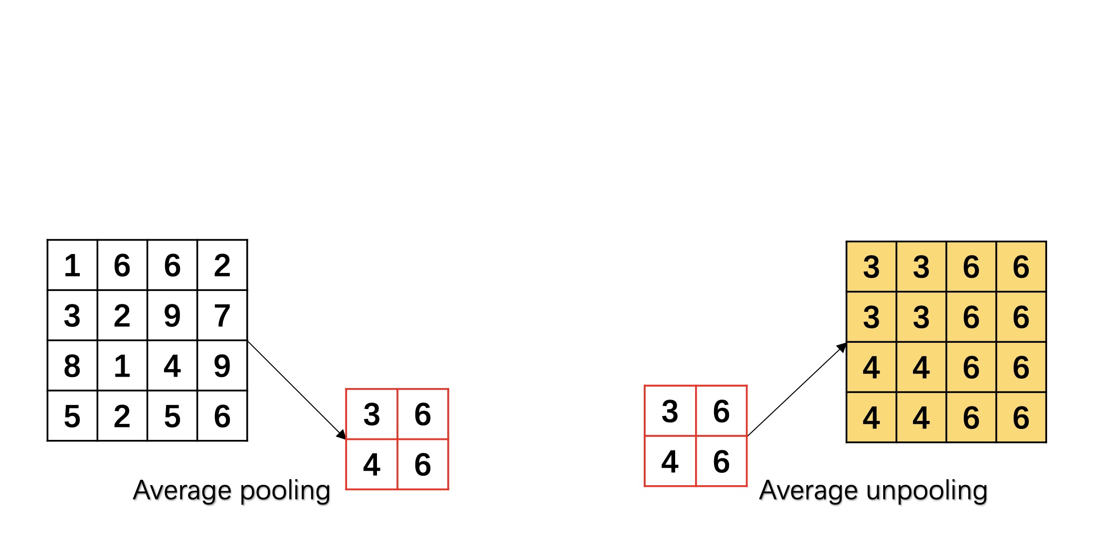
Further, auto-encoder [47, 48, 49] is used in order to retain the effective semantic information in . As shown in the right part of Fig 2, decoder is used to reconstruct from . It is made up of deconvolution, unpooling and fully connected layers. Among them, unpooling is the reverse of pooling and deconvolution is the reverse of convolution. Specifically, max unpooling keeps the maximum position information during max pooling, and then it restores the maximum values to the corresponding positions and set zeros to the rest positions as shown in Fig. 3(a). Analogously, average unpooling expands the feature map in the way of copying it as shown in Fig. 3(b).
The deconvolution is also called transpose convolution to recover the shape of input from output, as shown in Fig. 3(c). See appendix A for the detailed convolution and deconvolution Operation, as well as toy examples.
In addition, reconstruction loss is utilized to evaluate the difference between original signal data and reconstructed signal data.
| (5) |
where is the reconstruction of signal . Intuitively, the more complete signal is reconstructed, the more valid information is carried within . Thus, the auto-encoder greatly helps the model to generate appropriate semantic features.
As a result, the total loss function combines cross entropy loss, center loss and reconstruction loss as
| (6) |
where the weights and are used to balance the three loss functions. We have carefully designed the total loss function. The cross entropy loss is used to learn information from labels. And center loss minimizes the intra-class variations in the semantic space while keeping the inter-classes’ semantic features well separated, which also helps unknown classes to separate. Reconstruction loss makes model learn more information about signal data, because of well-reconstructed data. Ablation study in Section V also validates the above points. The whole learning process with loss is summarized in Algorithm 1, where , , denote the model parameters of the feature extractor , the classifier and the decoder , respectively.
IV-B Discriminator
The discriminator is the tail but the core of the proposed framework. It discriminates among known and unknown classes based on the latent semantic space . For each known class , the feature extractor extracts and computes the corresponding semantic center vector as:
| (7) |
where is the number of all training samples. When a test signal appears and is obtained, the difference between the vector and can be measured for each . Specifically, the generalized distance between and is used, which is defined as follows:
| (8) |
where is the transformation matrix associated with class and denotes the inverse of matrix . When is the covariance matrix of semantic features of signals of class , is called Mahalanobis distance. When is the identity matrix222This is also the only possible choice in the case when the covariance matrix is not available, which happens for example when the signal set of some class is singleton. , is reduced to Euclidean distance. also can be and where is a diagonal matrix formed by taking diagonal elements of and with being the dimension of . The corresponding distance based on and are called the second distance and third distance. Note that when the Mahalanobis distance, second distance and third distance are applied, the covariance matrix of each known class needs to be computed in advance.
With the above distance metric, we can establish our discriminant model which is divided into two steps. Firstly, distinguish between known and unknown classes. Secondly, discriminate which known classes or unknown classes the test signal belongs to. The first step is done by comparing the threshold with the minimal distance given by
| (9) |
where is the set of known semantic center vectors. Let us denote by the prediction of . If , , otherwise . Owing to utilizing the center loss in training, the semantic features of signals of class are assumed to obey multivariate Gaussian distribution. Inspired by the three-sigma rule [50], we set as follows
| (10) |
where is a control parameter referred to as the discrimination coefficient.
Two remarks are made as follows to explain the Gaussian distribution assumption and the choice of , respectively.
Remark 1
In our loss function, we have the center loss component which aims to minimize (2) with respect to the semantic layer. It is not difficult to show that
| (11) | ||||
Because of the monotonicity of exponential function, we have
| (12) | ||||
where denotes the dimension of Gaussian distribution and denotes the identity matrix. Let and , the above equation can be equivalently written as
| (13) |
where . This indicates that very likely the output of the semantic layer follows the Gaussian distribution.333Note that, however, due to the existence of the other two component loss functions, we propose using a general covariance matrix to describe the output of the semantic layer, as shown in (8).
Remark 2
The choice of in (10) is made due to the following two considerations. First, the well-known three-sigma rule of thumb is often used for identification of outliers [51]. It is shown in [51] that this rule should be properly generalized due to the impact of the dimension in the mult-dimensional case. We here present a natural generalization to the t-dimensional case by simply averaging the Mahalanobis distance over , so as to remove the impact of the dimension on the choice of . The above explains why we have the term in (10). Second, a control parameter is incorporated to make the choice of more sophisticated so that it can work well for complex recognition tasks. Our numerical experiments later validate the effectiveness of the choice of .
The second step is more complicated. If belongs to the known classes, its label can be easily obtained via
| (14) |
Obviously the main difficulty lies in dealing with the case when is classified as unknown in the first step. To illustrate, let us denote by the recorded unknown classes and define to be the set of the semantic center vectors of . In this difficult case with , a new signal label is added to and is set to be the semantic center vector . The unknown signal is saved in set and let . While in the difficult case with , the threshold is compared to the minimal distance which is defined by
| (15) |
total samples # of samples each class # of samples each SNR feature dimension classes (modulations) 220000 20000 1000 11 modulation types 8PSK, AM-DSB, AM-SSB, BPSK, CPFSK, GFSK, PAM4, QAM16, QAM64, QPSK, WBFM # of SNR values SNR values 20 -20,-18,-16,-14,-12,-10,-8,-6,-4,-2,0,2,4,6,8,10,12,14,16,18
Intuitively, a good choice of may be made based on the distance between and ’s. is the minimum distance which is firstly used in our test of choice of . Actually, we test a set of choices of and numerically find that unknown classes can be often correctly identified when is set between and , where is the median distance between and each . Therefore, the threshold is finally set as
| (16) |
where is used to balance the two distances and .
To proceed, let denote the number of recorded signal labels in . Then, if , a new signal label is added to and set . Note that we don’t impose any prior restrictions on the value of (the size of set ), i.e., our model can never know the number of the unknown classes pending to be discriminated. Then if , we set
| (17) |
and save the signal in . Accordingly, is updated via
| (18) |
where denotes the number of signals in set . As a result, with the increase of the number of predictions for unknown signals, the model will gradually improve itself by way of refining ’s.

To summarize, we present the whole procedure of the discriminator in Algorithm 2. We emphasize that our SR2CNN is different from the common open-set recognition methods. Assuming that there are known classes and an uncertain number of unknown classes, the traditional open-set recognition method will only distinguish the test samples into classes, while SR2CNN will distinguish the test samples into classes via Algorithm 2, where is the number of unknown classes recognized by the discriminator. Specifically, for the case when a test sample belongs to an unknown class, we determine whether it belongs to an existing unknown class or a new unknown class by comparing with threshold . Hence, the notable advantage of SR2CNN over the common open-set recognition method lies in that SR2CNN can roughly distinguish how many unknown classes there are in the test set, not just label the test sample as unknown.
V Experiments and Results
2016.10A 2016.10B 2016.04C supervised ZSL supervised ZSL supervised ZSL accuracy 8PSK (1) 85.0% 85.5% 95.5% 86.7% 74.9% 69.3% AM-DSB (2) 100.0% 73.5% 100.0% 41.3% 100.0% 91.1% BPSK (4) 99.0% 95.0% 99.8% 96.5% 99.8% 97.6% PAM4 (7) 98.5% 94.5% 97.6% 93.4% 99.6% 96.8% QAM16 (8) 41.6% 49.3% 56.8% 40.0% 97.6% 98.4% QAM64 (9) 60.6% 44.0% 47.5% 49.6% 94.0% 97.6% QPSK (10) 95.0% 90.5% 98.9% 90.6% 86.8% 81.5% WBFM (11) 38.2% 32.0% 39.6% 50.4% 88.8% 86.9% \cdashline6-6 CPFSK (5) 100.0% 99.0% 100.0% 75.9%/8.4% 100.0% 96.2% \cdashline4-4\cdashline8-8 GFSK (6) 100.0% 99.0% 100.0% 95.6%/2.3% 100.0% 82.0% AM-SSB (3) 100.0% 100.0% - - 100.0% 100.0% total accuracy 83.5% 78.4% 83.6% 72.0% 94.7% 91.5% average known accuracy 79.8% 73.7% 79.5% 68.5% 93.5% 91.6% true known rate - 95.9% - 86.9% - 97.0% true unknown rate - 99.5% - 91.1% - 90.0%

In this section, we demonstrate the effectiveness of the proposed SR2CNN approach by conducting extensive experiments with the dataset 2016.10A, as well as its two counterparts, 2016.10B and 2016.04C [15]. The data description is presented in Table I. All types of modulations are numbered with class labels from left to right.
Sieve samples. Samples with SNR less than 16 are firstly filtered out, only leaving a purer and higher-quality portion (one-tenth of origin) to serve as the overall datasets in our experiments.
Choose unknown classes. Empirically, a class whose features are hard to learn is an arduous challenge for a standard supervised learning model, let alone when it plays an unknown role in our ZSL scenario (especially when no prior knowledge about the number of the unknown classes is given, as we mentioned in the Subsection 4.2). Hence, necessarily, a completely supervised learning stage is carried out beforehand, to help us nominate suitable unknown classes. If the prediction accuracy of the full supervision method is rather low for certain class, it is reasonable to exclude this class in ZSL, because ZSL will definitely not yield a good performance for this class. In our experiments, unknown classes are randomly selected from a set of classes for which the accuracy of full supervision is higher than 50%. As shown in Table II, the ultimate candidates fall on AM-SSB(3) and GFSK(6) for 2016.10A and 2016.04C, while CPFSK(5) and GFSK(6) for 2016.10B.
Split training, validation and test data. 70% of the samples from the known classes make up the overall training set while 15% makes up the known validation set and the rest 15% makes up the known test set. For the unknown classes, there’s only a test set needed, which consists of 15% of the unknown samples.
Due to the three preprocessing steps, we get a small copy of, e.g., dataset 2016.10A, which contains a training set of samples, a known validation set of samples, a known test set of samples and an unknown test set of samples.
All of the networks in SR2CNN are computed on a single GTX Titan X graphic processor and implemented in Python, and trained using the Adam optimizer with learning rate and batch size . Generally, we allow our model to learn and update itself maximally for 250 epochs. In addition, the grid search is applied to the validation set to determine the hyperparameters.
V-A In-training Views
Basically, the average softmax accuracy of the known test set will converge roughly to on both 2016.10A and 2016.10B, while to on 2016.04C, as indicated in Fig. 4. Note that there’s almost no perceptible loss on the accuracy when using the clustering approach (i.e., the distance measure-based classification method described in Section IV) to predict instead of softmax, meaning that the semantic feature space established by our SR2CNN functions very well. For ease of exposition, we will refer to the known cluster accuracy as upbound (UB).
During the training course, the cross entropy loss undergoes sharp and violent oscillations. This phenomenon makes sense, since the extra center loss and reconstruction loss will intermittently shift the learning focus of the SR2CNN.
SR2CNN without Cross Entropy Loss without Center Loss without Reconstruction Loss L1 Loss accuracy AM-SSB(3) 100.0% 100.0% 99.5% 100.0% 100.0% GFSK(6) 99.5% 98.5% 61.0% 94.8% 95.8% average known accuracy 73.7% 72.1% 69.0% 72.3% 70.4% precision known 76.8% 75.3% 79.1% 74.5% 82.8% unknown 96.1% 95.2% 82.4% 94.5% 86.1% F1 score known 75.3% 73.6% 73.7% 73.3% 76.1% unknown 98.0% 97.2% 81.3% 95.9% 91.6%
V-B Critical Results
The most critical results are presented in Table II. To better illustrate it, we will firstly make a few definitions in analogy to the binary classification problem. By superseding the binary condition positive and negative with known and unknown respectively, we can similarly elicit true known (TK), true unknown (TU), false known (FK) and false unknown (FU). Subsequently, we get two important indicators as follows:
Furthermore, we define precision likewise as follows:
where denotes the total number of known samples that are classified to their exact known classes correctly. denotes the total number of unknown samples that are classified to their exact newly-identified unknown classes correctly. For evaluation, the real label of a certain newly-recorded unknown class is determined as the label of the most signal samples in that class. Note that sometimes unexpectedly, our SR2CNN may classify a small portion of signals into different unknown classes but their real labels are actually identical and correspond to one certain unknown class (we name these unknown classes as isotopic classes). In this rare case, we only count the identified unknown class with the highest accuracy in calculating .
For ZSL, we test our SR2CNN with several different combinations of aforementioned parameters and , hopefully to snatch a certain satisfying result out of multiple trials. Fixing to 1 simply leads to fair performance, though still, we adjust in a range between 0.05 and 1.0. Here, the pre-defined indicators above play an indispensable part to help us sift the results. Generally, a well-chosen result is supposed to meet the following requirements: 1. the weighted true rate (WTR): TKR+TUR is as great as possible; 2. KPUB, where UB is the upbound defined as the known cluster accuracy; 3. 2 for all possible , where denotes the number of isotopic classes corresponding to a certain unknown class .

unknown classes AM-SSB and GFSK CPFSK and GFSK AM-SSB and CPFSK AM-SSB, CPFSK and GFSK accuracy AM-SSB(3) 100.0% - 100.0% 100.0% CPFSK(5) - 71.0% 87.8%/9.0% 65.5% GFSK(6) 99.5% 100.0% - 90.5% average known accuracy 73.7% 68.3% 75.6% 69.6% true known rate 95.9% 89.6% 96.2% 90.9% true unknown rate 99.8% 85.5% 98.4% 85.4% precision known 76.8% 73.6% 78.3% 74.0% unknown 96.1% 89.2% 91.9% 90.4%
In order to better make a transverse comparision, we compute two extra indicators, average total accuracy in ZSL scenario and also average known accuracy in completely supervised learning, shown as italics in Table II. On the whole, the results are promising and excellent. However, we have to admit that ZSL learning somewhat incurs a little bit performance loss as compared with the fully supervised model. Looking vertically, among all modulations, the performance loss especially occurs in the class AM-DSB. While looking horizontally among all datasets, the performance loss especially occurs in dataset 2016.10B. After all, when losing sight of the two unknown classes, SR2CNN can only acquire a segment of the intact knowledge that shall be totally learned in a supervised case. It is this imperfection that presumably leads to an apparent variation on each class’s accuracy when compared with supervised learning. Among these classes, the poorest victim is always AM-DSB, with considerable portion of its samples rejected as unknown ones. Besides, the features, especially those of the unknown classes, among these three datasets are not exactly in the same difficulty levels of learning. Some unknown features may even be similar to those known ones, which can consequently cause confusions in the discrimination tasks. It is no doubt that these uncertainties and differences in the feature domain matter a lot. Take 2016.10B, compared with its two counterparts, it emanates the greatest loss (more than 10%) on average accuracy (both total and known), and also a pair of inferior true rates. Moreover, it is indeed the single case, where both two unknown classes are separately identified into two isotopic classes.
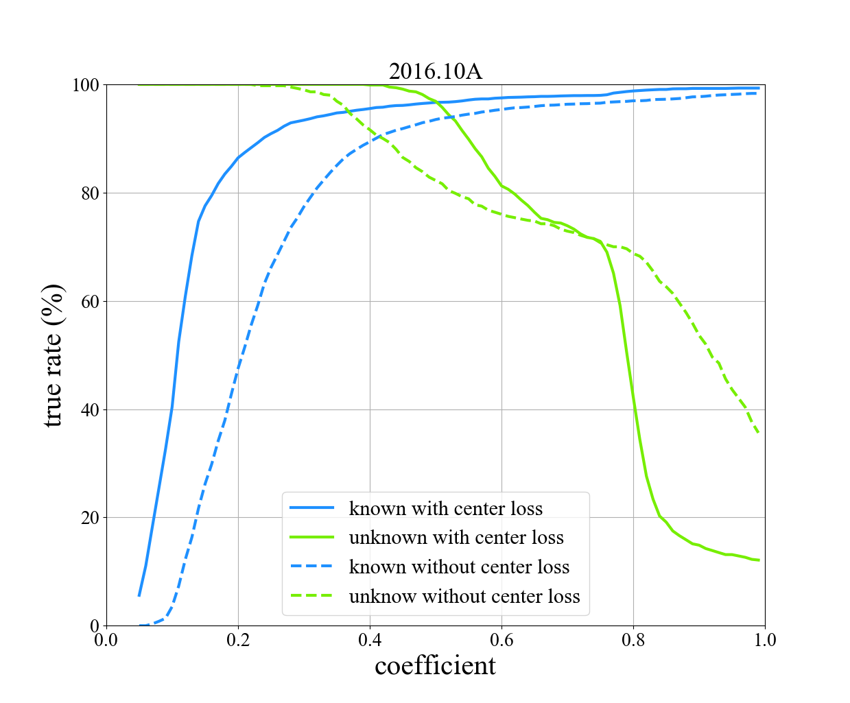
It is obvious that average accuracy strongly depends on the weighted true rate (WTR). Since the clearer for the discrimination between known and unknown, the more accurate for the further classification and identification. Therefore, to better study this discrimination ability, we depict Fig. 5 to elucidate its variation trends regarding discrimination coefficient (). At the same time, we introduce a new concept discrimination interval as an interval where the weighted true rate is always greater than 80%. The width of the above interval is used to help quantify this discrimination ability.
SR2CNN IsolationForest [37] EllipticEnvelope [38] OneClassSVM [39] LocalOutlierFactor [40] OpenMax [8] MDL4OW [43] AM-SSB(3) 100.0% 72.3% 00.0% 100.0% 100.0% 96.3% 26.0% 100.0% 100.0% 99.3% GFSK(6) 99.5% 01.3% 00.0% 90.0% 00.0% 00.0% 00.0% 00.0% 00.0% 26.5% true known rate 95.9% 81.3% 99.9% 46.1% 97.6% 85.5% 92.0% 96.7% 98.1% 79.4% true unknown rate 99.8% 36.8% 00.0% 95.0% 50.0% 48.1% 13.0% 50.0% 50.0% 62.9%
SIGNAL-202002 supervised learning zero-shot learning accuracy BPSK (1) 84.3% 70.8% QPSK (2) 86.5% 67.8% 8PSK (3) 67.8% 70.3% 16QAM (4) 99.5% 96.8% 64QAM (5) 95.5% 84.8% PAM4 (6) 97.0% 89.0% GFSK (7) 56.3% 38.3% AM-DSB (10) 63.8% 67.3% AM-SSB (11) 44.3% 62.0% \cdashline4-4 CPFSK (8) 100.0% 81.0% B-FM (9) 93.5% 74.5% average total accuracy 80.8% 73.0% average known accuracy 77.3% 71.9% true known rate - 82.3% true unknown rate - 84.9% precision known - 87.4% unknown - 91.6%
Apparently, the curves for the primary two kinds of true rate are monotonic, increasing for the known while decreasing for the unknown. The maximum points of these weighted true rate curves for each dataset, are about 0.4, 0.2, and 0.4 respectively. These points exactly correspond to the results shown in Table II. Besides, the width of the discrimination interval of 2016.10B is only approximately one third of those of 2016.10A and 2016.04C. This implies that the features of 2016.10B are more difficult to learn, and just accounts for its relatively poor performance.
V-C Ablation Study
In this subsection, we explain the necessity of each of the three loss functions. Relevant experiments are mainly based on 2016.10A.
Fig. 6 presents the known accuracy in absence of cross entropy loss, center loss and reconstruction loss respectively during training. In general, we found that the best performance in training will be degraded when any one of these three loss functions is excluded. It can be observed that both cross entropy loss and reconstruction loss make a positive impact on the known accuracy, boosting about 3% to 5%, while center loss seems slightly weaker.
Analyzing Table III, we can easily discern the effect of these three loss functions in the test course, especially the center loss. Results show that the F1 score in absence of cross entropy loss, center loss and reconstruction loss decreases by 1.8%, 1.7% and 2.0% respectively for the known classes. For the unknown classes, the minimum degradation in F1 score is 0.8% after removing cross entropy loss, while the maximum degradation in F1 score is 16.7% after removing center loss. Actually, Fig. 7 indicates that the usage of center loss on 2016.10A indeed helps our model to discriminate more distinctly, resulting in a notably broader discrimination interval. Besides, we have also made an attempt at applying L1 loss [52] to calculate center loss (Eq. (2) in Section IV) and reconstruction loss (Eq. (5) in Section IV). Those related results are presented in the last column of Table III. It is seen that L1 loss can indeed slightly increase the F1 score of known classes by 0.8%, however, at the cost of a decrease in the F1 score of unknown classes by 6.4%.
In sum, the three loss functions, though not exactly promoting our SR2CNN in the same way and in the same fields, are indeed useful.
V-D Other Extensions
We tentatively change several unknown classes on 2016.10A, seeking to excavate more in the feature domain of data. As shown in Table IV, both known precision (KP) and unknown precision (UP) are insensitive to the change of unknown classes, proving that the classification ability of SR2CNN are consistent and well-preserved for the considered dataset. Nevertheless, obviously, the unknown class CPFSK is always the hardest obstacle in the course of discrimination. Since accuracy of CPFSK is always the lowest as well as some isotopic classes are observed in this case. Especially, when class CPFSK and GFSK simultaneously show up in the unknown roles, the performance loss (on both TKR and TUR) is quite striking. We speculate that the unknown CPFSK and GFSK may share a considerable number of similarities with some known classes, which will unluckily mislead SR2CNN about the further discrimination task.
To justify SR2CNN’s superiority, we compare it with a couple of traditional methods prevailing in the field of outlier detection, as well as two open-set recognition methods, i.e., OpenMax [8] and MDL4OW [43]. For outlier detection methods, the detected outlier will be regarded as an unknown sample. For OpenMax, an extra dimension is appended to the output vector to indicate the probability of the current sample being unknown. While for MDL4OW, the extreme value theory is adopted to detect the unknown classes by modeling the distribution of loss. The results are presented in Table V. It is found that our SR2CNN significantly outperforms both outlier detection methods and open-set recognition methods in terms of the true unknown rate. Furthermore, we find that most of the aforementioned methods cannot correctly identify GFSK as unknown. For example, in our experiment, OpenMax wrongly classifies all GFSK samples as known. As for MDL4OW, it identifies a small percentage of GFSK samples at the cost of true known rate. However, it can be found from the experiment results that our SR2CNN can still work very well for this open-set recognition task.
Note that there are no unknown classes identification tasks launched, only discrimination tasks are considered. Hence, here, for a certain unknown class , we compute its unknown rate, instead of accuracy, as , where denotes the number of samples from unknown class , while denotes the number of samples from unknown class , which are discriminated as unknown ones.

In addition, relevant ROC curves for the above comparison experiments are depicted in Fig. 8. It is observed that SR2CNN has the largest AUC, indicating its superiority over other methods. Besides, notably, there seems as if a steep ‘cliff erecting’ where False Known Rate approximately equals to 0.5, particularly for EllipticEnvelope, LocalOutlierFactor, and OpenMax. This means that almost half samples of unknown classes are not easy to be correctly discriminated. Correspondingly, according to Table V, we can speculate that these ‘hard’ samples all come from unknown class GFSK.
VI Dataset SIGNAL-202002
We newly synthesize a dataset, denominated as SIGNAL-202002, to hopefully be of great use for further researches in signal recognition field. Basically, the dataset consists of 11 modulation types, which are BPSK, QPSK, 8PSK, 16QAM, 64QAM, PAM4, GFSK, CPFSK, B-FM, AM-DSB and AM-SSB. Each type is composed of 20000 frames. Data is modulated at a rate of 8 samples per symbol, while 128 samples per frame. The channel impairments are modeled by a combination of additive white Gaussian noise, Rayleigh fading, multipath channel and clock offset. We pass each frame of our synthetic signals independently through the above channel model, seeking to emulate the real-world case, which shall consider translation, dilation and impulsive noise, etc. The configuration is set as follows:
20000 samples per modulation type
feature dimension
20 different SNRs, even values between [2dB, 40dB]
The complete dataset is stored as a python pickle file which is about 450 MBytes in complex 32 bit floating point type. Related code for the generation process is implemented in MatLab and the SIGNAL-202002 dataset is available on the link: https://drive.google.com/file/d/1EDfKRNIk_txxyAyPCR7BEGs0BvEk3Bof/view.
We conduct zero-shot learning experiments on our newly-generated dataset and report the results here. As mentioned above, a supervised learning trial is similarly carried out to help us get an overview of the regular performance for each class of SIGNAL-202002. Unfortunately, as Table VI shows, the original two candidates of 2016.10A, AM-SSB and GFSK, both fail to keep on top. Therefore, here, we relocate the unknown roles to another two modulations, CPFSK with the highest accuracy overall, as well as B-FM, which stands out in the three analogy modulation types (B-FM, AM-SSB and AM-DSB).
According to Table VI, an apparent loss on the discrimination ability is observed, as both the TKR and the TUR just slightly pass 80%. However, our SR2CNN still maintain its classification ability, as the accuracy for each class remains encouraging compared with the completely-supervised model. A significant fact is that, the known precision (KP) is incredibly high, even exceeding those KPs on 2016.10A by almost 10%, as shown in Table IV. To account for this, we speculate that the absence of two unknown classes may unintentionally allow SR2CNN to better focus on the features of the known ones, which consequently, leads to a superior performance of known classification task.
VII Conclusion
In this paper, we have proposed a ZSL framework SR2CNN, which can successfully extract precise semantic features of signals and discriminate both known classes and unknown classes. SR2CNN can works very well in the situation where we have no sufficient training data for certain class. Moreover, SR2CNN can generally improve itself in the way of updating semantic center vectors. Extensive experiments demonstrate the effectiveness of SR2CNN. In addition, we provide a new signal dataset SIGNAL-202002 including eight digital and three analog modulation classes for further research. Finally, we would like to point out that, because we often have I/Q signals, a possible direction for future research is using complex neural networks [53] to establish the semantic space.
Appendix A Convolution and Deconvolution Operation
Let denote the vectorized input and output matrices. Then the convolution operation can be expressed as
| (19) |
where denotes the convolutional matrix, which is sparse. With back propagation of convolution, is obtained, thus
| (20) |
where denotes the -th element of , denotes the -th element of , denotes the element in the i-th row and j-th column of , and denotes the -th column of . Hence,
| (21) |
Similarly, the deconvolution operation can be notated as
| (22) |
where denotes a convolutional matrix that has the same shape as , and it needs to be learned. Then the back propagation of convolution can be formulated as follows:
| (23) |
For example, the size of the input and output matrices is and as shown in Fig. 3(c). Then is a 16-dimensional vector and is a 4-dimensional vector. Define convolutional kernel as
| (24) |
It is not hard to imagine that is a matrix, and it can be represented as follows:
| (25) |
Hence, deconvolution is expressed as left-multiplying in forward propagation, and left-multiplying in back propagation.
References
- [1] T. J. O’Shea, T. Roy, and T. C. Clancy, “Over-the-air deep learning based radio signal classification,” IEEE Journal of Selected Topics in Signal Processing, vol. 12, no. 1, pp. 168–179, 2018.
- [2] F. Gama, A. G. Marques, G. Leus, and A. Ribeiro, “Convolutional neural network architectures for signals supported on graphs,” IEEE Transactions on Signal Processing, vol. 67, no. 4, pp. 1034–1049, 2018.
- [3] S. Peng, H. Jiang, H. Wang, H. Alwageed, Y. Zhou, M. M. Sebdani, and Y.-D. Yao, “Modulation classification based on signal constellation diagrams and deep learning,” IEEE transactions on neural networks and learning systems, vol. 30, no. 3, pp. 718–727, 2018.
- [4] T. J. O’Shea, J. Corgan, and T. C. Clancy, “Unsupervised representation learning of structured radio communication signals,” in 2016 First International Workshop on Sensing, Processing and Learning for Intelligent Machines (SPLINE). IEEE, 2016, pp. 1–5.
- [5] L. Du, H. Liu, P. Wang, B. Feng, M. Pan, and Z. Bao, “Noise robust radar hrrp target recognition based on multitask factor analysis with small training data size,” IEEE Transactions on Signal Processing, vol. 60, no. 7, pp. 3546–3559, 2012.
- [6] G. C. Garriga, P. Kralj, and N. Lavrač, “Closed sets for labeled data,” Journal of Machine Learning Research, vol. 9, no. Apr, pp. 559–580, 2008.
- [7] W. J. Scheirer, A. de Rezende Rocha, A. Sapkota, and T. E. Boult, “Toward open set recognition,” IEEE transactions on pattern analysis and machine intelligence, vol. 35, no. 7, pp. 1757–1772, 2012.
- [8] A. Bendale and T. E. Boult, “Towards open set deep networks,” in Proceedings of the IEEE conference on computer vision and pattern recognition, 2016, pp. 1563–1572.
- [9] H. Liu, Z. Cao, M. Long, J. Wang, and Q. Yang, “Separate to adapt: Open set domain adaptation via progressive separation,” in Proceedings of the IEEE Conference on Computer Vision and Pattern Recognition, 2019, pp. 2927–2936.
- [10] C. Geng and S. Chen, “Collective decision for open set recognition,” IEEE Transactions on Knowledge and Data Engineering, 2020.
- [11] M. Palatucci, D. Pomerleau, G. E. Hinton, and T. M. Mitchell, “Zero-shot learning with semantic output codes,” in Advances in neural information processing systems, 2009, pp. 1410–1418.
- [12] R. Socher, M. Ganjoo, C. D. Manning, and A. Ng, “Zero-shot learning through cross-modal transfer,” in Advances in neural information processing systems, 2013, pp. 935–943.
- [13] Z. Wang, X. Ye, C. Wang, J. Cui, and P. Yu, “Network embedding with completely-imbalanced labels,” IEEE Transactions on Knowledge and Data Engineering, 2020.
- [14] Y. Gao, L. Gao, X. Li, and Y. Zheng, “A zero-shot learning method for fault diagnosis under unknown working loads,” Journal of Intelligent Manufacturing, pp. 1–11, 2019.
- [15] T. J. O’Shea, J. Corgan, and T. C. Clancy, “Convolutional radio modulation recognition networks,” in International conference on engineering applications of neural networks. Springer, 2016, pp. 213–226.
- [16] K. He, X. Zhang, S. Ren, and J. Sun, “Deep residual learning for image recognition,” in Proceedings of the IEEE conference on computer vision and pattern recognition, 2016, pp. 770–778.
- [17] S. Zheng, S. Chen, L. Yang, J. Zhu, Z. Luo, J. Hu, and X. Yang, “Big data processing architecture for radio signals empowered by deep learning: Concept, experiment, applications and challenges,” IEEE Access, vol. 6, pp. 55 907–55 922, 2018.
- [18] B. Flowers, R. M. Buehrer, and W. C. Headley, “Evaluating adversarial evasion attacks in the context of wireless communications,” IEEE Transactions on Information Forensics and Security, vol. 15, pp. 1102–1113, 2019.
- [19] S. Duan, K. Chen, X. Yu, and M. Qian, “Automatic multicarrier waveform classification via pca and convolutional neural networks,” IEEE Access, vol. 6, pp. 51 365–51 373, 2018.
- [20] L. J. Wong, W. C. Headley, and A. J. Michaels, “Specific emitter identification using convolutional neural network-based iq imbalance estimators,” IEEE Access, vol. 7, pp. 33 544–33 555, 2019.
- [21] S. Huang, L. Chai, Z. Li, D. Zhang, Y. Yao, Y. Zhang, and Z. Feng, “Automatic modulation classification using compressive convolutional neural network,” IEEE Access, vol. 7, pp. 79 636–79 643, 2019.
- [22] S. Dörner, S. Cammerer, J. Hoydis, and S. ten Brink, “Deep learning based communication over the air,” IEEE Journal of Selected Topics in Signal Processing, vol. 12, no. 1, pp. 132–143, 2017.
- [23] L. M. Hoang, M. Kim, and S.-H. Kong, “Automatic recognition of general lpi radar waveform using ssd and supplementary classifier,” IEEE Transactions on Signal Processing, vol. 67, no. 13, pp. 3516–3530, 2019.
- [24] G. Vanhoy, N. Thurston, A. Burger, J. Breckenridge, and T. Bose, “Hierarchical modulation classification using deep learning,” in MILCOM 2018-2018 IEEE Military Communications Conference (MILCOM). IEEE, 2018, pp. 20–25.
- [25] T. J. O’Shea, T. Roy, N. West, and B. C. Hilburn, “Demonstrating deep learning based communications systems over the air in practice,” in 2018 IEEE International Symposium on Dynamic Spectrum Access Networks (DySPAN). IEEE, 2018, pp. 1–2.
- [26] G. Baldini, C. Gentile, R. Giuliani, and G. Steri, “Comparison of techniques for radiometric identification based on deep convolutional neural networks,” Electronics Letters, vol. 55, no. 2, pp. 90–92, 2018.
- [27] S. M. Hiremath, S. Behura, S. Kedia, S. Deshmukh, and S. K. Patra, “Deep learning-based modulation classification using time and stockwell domain channeling,” in 2019 National Conference on Communications (NCC). IEEE, 2019, pp. 1–6.
- [28] X. Zhang, T. Seyfi, S. Ju, S. Ramjee, A. El Gamal, and Y. C. Eldar, “Deep learning for interference identification: Band, training snr, and sample selection,” in 2019 IEEE 20th International Workshop on Signal Processing Advances in Wireless Communications (SPAWC). IEEE, 2019, pp. 1–5.
- [29] K. Sankhe, M. Belgiovine, F. Zhou, L. Angioloni, F. Restuccia, S. D’Oro, T. Melodia, S. Ioannidis, and K. Chowdhury, “No radio left behind: Radio fingerprinting through deep learning of physical-layer hardware impairments,” IEEE Transactions on Cognitive Communications and Networking, vol. 6, no. 1, pp. 165–178, 2019.
- [30] F. Liang, C. Shen, W. Yu, and F. Wu, “Towards optimal power control via ensembling deep neural networks,” IEEE Transactions on Communications, vol. 68, no. 3, pp. 1760–1776, 2019.
- [31] X. Chen, J. Cheng, Z. Zhang, L. Wu, J. Dang, and J. Wang, “Data-rate driven transmission strategies for deep learning-based communication systems,” IEEE Transactions on Communications, vol. 68, no. 4, pp. 2129–2142, 2020.
- [32] D. Roy, T. Mukherjee, M. Chatterjee, E. Blasch, and E. Pasiliao, “Rfal: Adversarial learning for rf transmitter identification and classification,” IEEE Transactions on Cognitive Communications and Networking, 2019.
- [33] J. Tan, L. Zhang, Y.-C. Liang, and D. Niyato, “Intelligent sharing for lte and wifi systems in unlicensed bands: A deep reinforcement learning approach,” IEEE Transactions on Communications, vol. 68, no. 5, pp. 2793–2808, 2020.
- [34] M. Li, O. Li, G. Liu, and C. Zhang, “Generative adversarial networks-based semi-supervised automatic modulation recognition for cognitive radio networks,” Sensors, vol. 18, no. 11, p. 3913, 2018.
- [35] M. Usama, J. Qadir, A. Raza, H. Arif, K.-L. A. Yau, Y. Elkhatib, A. Hussain, and A. Al-Fuqaha, “Unsupervised machine learning for networking: Techniques, applications and research challenges,” IEEE Access, vol. 7, pp. 65 579–65 615, 2019.
- [36] Z.-L. Tang, S.-M. Li, and L.-J. Yu, “Implementation of deep learning-based automatic modulation classifier on FPGA SDR platform,” Electronics, vol. 7, no. 7, p. 122, 2018.
- [37] F. T. Liu, K. M. Ting, and Z.-H. Zhou, “Isolation forest,” in 2008 Eighth IEEE International Conference on Data Mining. IEEE, 2008, pp. 413–422.
- [38] P. J. Rousseeuw and K. V. Driessen, “A fast algorithm for the minimum covariance determinant estimator,” Technometrics, vol. 41, no. 3, pp. 212–223, 1999.
- [39] Y. Chen, X. S. Zhou, and T. S. Huang, “One-class SVM for learning in image retrieval,” in Proceedings 2001 International Conference on Image Processing (Cat. No. 01CH37205), vol. 1. IEEE, 2001, pp. 34–37.
- [40] M. M. Breunig, H.-P. Kriegel, R. T. Ng, and J. Sander, “Lof: identifying density-based local outliers,” in Proceedings of the 2000 ACM SIGMOD international conference on Management of data, 2000, pp. 93–104.
- [41] R. Yoshihashi, W. Shao, R. Kawakami, S. You, M. Iida, and T. Naemura, “Classification-reconstruction learning for open-set recognition,” in Proceedings of the IEEE Conference on Computer Vision and Pattern Recognition, 2019, pp. 4016–4025.
- [42] C. Geng, S.-j. Huang, and S. Chen, “Recent advances in open set recognition: A survey,” IEEE Transactions on Pattern Analysis and Machine Intelligence, 2020.
- [43] S. Liu, Q. Shi, and L. Zhang, “Few-shot hyperspectral image classification with unknown classes using multitask deep learning,” IEEE Transactions on Geoscience and Remote Sensing, 2020.
- [44] D. Roy, T. Mukherjee, M. Chatterjee, and E. Pasiliao, “Detection of rogue RF transmitters using generative adversarial nets,” in 2019 IEEE Wireless Communications and Networking Conference (WCNC). IEEE, 2019, pp. 1–7.
- [45] S. Rajendran, W. Meert, V. Lenders, and S. Pollin, “Saife: Unsupervised wireless spectrum anomaly detection with interpretable features,” in 2018 IEEE International Symposium on Dynamic Spectrum Access Networks (DySPAN). IEEE, 2018, pp. 1–9.
- [46] Y. Wen, K. Zhang, Z. Li, and Y. Qiao, “A discriminative feature learning approach for deep face recognition,” in European conference on computer vision. Springer, 2016, pp. 499–515.
- [47] X. Chen, D. P. Kingma, T. Salimans, Y. Duan, P. Dhariwal, J. Schulman, I. Sutskever, and P. Abbeel, “Variational lossy autoencoder,” arXiv preprint arXiv:1611.02731, 2016.
- [48] I. Higgins, L. Matthey, A. Pal, C. Burgess, X. Glorot, M. Botvinick, S. Mohamed, and A. Lerchner, “beta-vae: Learning basic visual concepts with a constrained variational framework.” ICLR, vol. 2, no. 5, p. 6, 2017.
- [49] A. Ng et al., “Sparse autoencoder,” CS294A Lecture notes, vol. 72, no. 2011, pp. 1–19, 2011.
- [50] F. Pukelsheim, “The three sigma rule,” The American Statistician, vol. 48, no. 2, pp. 88–91, 1994.
- [51] P. Bajorski, Statistics for imaging, optics, and photonics. John Wiley & Sons, 2011, vol. 808.
- [52] H. Zhao, O. Gallo, I. Frosio, and J. Kautz, “Loss functions for image restoration with neural networks,” IEEE Transactions on Computational Imaging, vol. 3, no. 1, pp. 47–57, 2017.
- [53] A. Hirose, Complex-valued neural networks: Advances and applications. John Wiley & Sons, 2013, vol. 18.
![[Uncaptioned image]](https://cdn.awesomepapers.org/papers/3b112fbe-a06f-42a5-8a91-1a5b72b95d09/dyh.jpeg) |
Yihong Dong received his B.S. degree in Computer Science from Shanghai University, China, in 2019. He is currently a graduate student with the School of Software Engineering, Tongji University. His research interests include machine learning with the applications in signal processing. |
![[Uncaptioned image]](https://cdn.awesomepapers.org/papers/3b112fbe-a06f-42a5-8a91-1a5b72b95d09/jxh.jpeg) |
Xiaohan jiang is currently an undergraduate with the School of Software Engineering, Tongji University. His research interests include deep learning and computer vision. |
![[Uncaptioned image]](https://cdn.awesomepapers.org/papers/3b112fbe-a06f-42a5-8a91-1a5b72b95d09/zhj.jpg) |
Huaji Zhou was born in Jinhua, Zhejiang, China, in 1988. He received the B.S. degree in Navigation, Guidance, and Control Technology and the M.S. degree in Pattern Recognition and Intelligent System from Xidian University, Xi’an, China, in 2010 and 2013, respectively. He is currently a Research Assistant with Science and Technology on Communication Information Security Control Laboratory, Jiaxing, China. And he is pursuing Ph.D. degree in Electronics and Information at Xidian University, Xi’an, China, His current research interests include machine learning and electromagnetic signal processing. |
![[Uncaptioned image]](https://cdn.awesomepapers.org/papers/3b112fbe-a06f-42a5-8a91-1a5b72b95d09/ly.jpeg) |
Yun Lin received the B.S. degree from Dalian Maritime University, Dalian, China, in 2003, the M.S. degree from the Harbin Institute of Technology, Harbin, China, in 2005, and the Ph.D. degree from Harbin Engineering University, Harbin, China, in 2010. He was a research scholar with Wright State University, USA, from 2014 to 2015. Now, he is currently a full professor in the College of Information and Communication Engineering, Harbin Engineering University, China. His current research interests include machine learning and data analytics over wireless networks, signal processing and analysis, cognitive radio and software defined radio, artificial intelligence and pattern recognition. He had published more than 150 international peer-reviewed journal/conference papers, such as the IEEE IoT, TII, TVT, TCCN, TR, Access, INFOCOM, GLOBECOM, ICC, VTC, ICNC. He had four high-cited papers and several best conference papers. He is serving as an editor for the IEEE TRANSACTIONS ON RELIABILITY, KSII Transactions on Internet and Information Systems, and International Journal of Performability Engineering. In addition, he served as General Chair of ADHIP 2020, TPC Chair of MOBIMEDIA 2020, ICEICT 2019 and ADHIP 2017, and TPC member of GLOBECOM, ICC, ICNC and VTC. He had successfully organized several international workshops and symposia with top‐ranked IEEE conferences, including INFOCOM, GLOBECOM, DSP, ICNC, among others. |
![[Uncaptioned image]](https://cdn.awesomepapers.org/papers/3b112fbe-a06f-42a5-8a91-1a5b72b95d09/sqj.png) |
Qingjiang Shi received his Ph.D. degree in electronic engineering from Shanghai Jiao Tong University, Shanghai, China, in 2011. From September 2009 to September 2010, he visited Prof. Z.-Q. (Tom) Luo’s research group at the University of Minnesota, Twin Cities. In 2011, he worked as a Research Scientist at Bell Labs China. From 2012, He was with the School of Information and Science Technology at Zhejiang Sci-Tech University. From Feb. 2016 to Mar. 2017, he worked as a research fellow at Iowa State University, USA. From Mar. 2018, he is currently a full professor with the School of Software Engineering at Tongji University. He is also with the Shenzhen Research Institute of Big Data. His interests lie in algorithm design and analysis with applications in machine learning, signal processing and wireless networks. So far he has published more than 60 IEEE journals and filed about 30 national patents. Dr. Shi was an Associate Editor for the IEEE TRANSACTIONS ON SIGNAL PROCESSING. He was awarded Golden Medal at the 46th International Exhibition of Inventions of Geneva in 2018, and also was the recipient of the First Prize of Science and Technology Award from China Institute of Communications in 2018, the National Excellent Doctoral Dissertation Nomination Award in 2013, the Shanghai Excellent Doctorial Dissertation Award in 2012, and the Best Paper Award from the IEEE PIMRC’09 conference. |