Spin-dependent edge states in two-dimensional Dirac materials with a flat band

Li-Li Ye School of Electrical, Computer and Energy Engineering, Arizona State University, Tempe, Arizona 85287, USA Chen-Di Han School of Electrical, Computer and Energy Engineering, Arizona State University, Tempe, Arizona 85287, USA Ying-Cheng Lai [email protected] School of Electrical, Computer and Energy Engineering, Arizona State University, Tempe, Arizona 85287, USA Department of Physics, Arizona State University, Tempe, Arizona 85287, USA

(December 6, 2024)

Abstract

The phenomenon of spin-dependent quantum scattering in two-dimensional (2D) pseudospin-1/2 Dirac materials leading to a relativistic quantum chimera was recently uncovered. We investigate spin-dependent Dirac electron optics in 2D pseudospin-1 Dirac materials, where the energy-band structure consists of a pair of Dirac cones and a flat band. In particular, with a suitable combination of external electric fields and a magnetic exchange field, electrons with a specific spin orientation (e.g., spin-down) can be trapped in a class of long-lived edge modes, generating resonant scattering. The spin-dependent edge states are a unique feature of flat-band Dirac materials and have no classical correspondence. However, electrons with the opposite spin (i.e., spin up) undergo conventional quantum scattering with a classical correspondence, which can be understood in the framework of Dirac electron optics. A consequence is that the spin-down electrons produce a large scattering probability with broad scattering angle distribution in both near- and far-field regions, while the spin-up electrons display the opposite behavior. Such characteristically different behaviors of the electrons with opposite spins lead to spin polarization that can be as high as nearly 100%.

I Introduction

Dirac electron optics can be demonstrated by the behaviors of ballistic electrons in the paradigmatic graphene p-n junction system [1]. Specifically, due to the relativistic quantum phenomenon of Klein tunneling and the gapless Dirac cone dispersion relation, the transmission of Dirac electrons through the p-n junction interface resembles a highly transparent focusing lens with negative refractive index [2], corresponding to a Vaselago lens [3] for chiral Dirac fermions in graphene. It provides an experimental approach to tuning the refractive index through varying the gate potential, making it possible to realize graphene-based electronic lens [4] and graphene transistors [5]. In Dirac electron optics, various electronic counterparts of optical phenomena have been achieved such as Fabry-Pérot resonances [6, 7], cloaking [8], Dirac fermion microscope [9], electron Mie scattering [10, 11, 12, 13, 14]. In addition, in the framework of Dirac electron optics, diverse unconventional relativistic quantum phenomena such as anti-super-Klein tunneling in phosphorene p-n junctions [1] and tilted energy dispersion effect [15] have been studied. A rigorous semiclassical theory beyond the standard WKB approximation for the two-dimensional (2D) Dirac equation was developed [16] as the foundation of Dirac electron optics. Experimentally, Dirac fermion flows were imaged through a circular Veselago lens using the polarized tip of a scanning gate microscope [17] and nanoscale quantum electron optics was tested in graphene with atomically sharp p-n junctions [18].

The magnetic exchange field(MEF) provides a natural testbed for the spin-dependent Dirac electron optics. It can be induced by the adjacent magnetic insulator, i.e. 2D-material/magnetic insulator, incorporating EuS [19], and ferromagnetic insulator(FMI) [20], and it enables the efficient control [21, 22] of spin generation and modulation in 2D-materials. Moreover, the MEF in magnetic multilayers is promising to achieve tens or even hundreds of tesla [23, 19]. The spin-dependent electronic spin lens [24], i.e. the counterpart of the photonic chiral metamaterials, generated by the spin-resolved negative refraction Klein tunneling, has been discussed with the magnetic exchange field in graphene normal-ferromagnetic-normal configuration. It spurs the growth of research about electron optics [25, 26, 27, 28, 2, 29, 30, 31]. In Dirac quantum chimera state [2] with MEF interaction, the unusual spin-resolved coexistence states by classically chaotic and integral optical quasibound states have been discovered in the annular cavity made with pseudospin-1/2 Dirac fermions, which have the features about the enhancement of Dirac electron spin polarization.

In this work, we explore spin-dependent edge modes in pseudospin-1 Dirac materials by the electrostatic field and MEF interaction. In the previous work [32, 33], a class of robust edge modes arises that can resist even fully developed classical chaos and Klein tunneling [32, 33] - a unique feature of pseudospin-1 Dirac materials in the absence of a magnetic exchange potential so that the real spin degrees of freedom are degenerate. (It is plausible that such edge modes possess certain topological features [34, 35].) Based on this, we demonstrate that systems of pseudospin-1 Dirac materials with a flat band represent an intriguing manifestation of the coexistence in electronic quasibound states of classic lensing(integrable or chaotic states) and non-classical edge states. The former displays electron-optic scattering and the latter demonstrates unconventional scattering. Between that, the interplay features have been explored, and it achieves nearly 100% spin polarization.

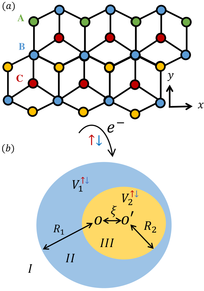
Compared with graphene, pseudospin-1 Dirac material systems are capable of delivering unconventional physical phenomena such as super-Klein tunneling [36], novel conical diffraction [37, 38, 39] and chaos Q-spoiling defiance with edge states [32]. An example of pseudospin-1 materials is the dice lattice, as shown in Fig. 1(a), where the quasiparticles can be described by the generalized 2D Dirac-Weyl Hamiltonian [40]. Consider an eccentric circular cavity of dice lattice consisting of a large circle and a small circular domain inside the large one, where the centers of the two circles do not coincide, as illustrated in Fig. 1(b). The real spin degree of freedom of electron carries becomes relevant when the whole device is placed on a ferromagnetic substrate [19, 20], as described by a magnetic exchange potential in the Hamiltonian. Now apply two distinct gate voltages to the cavity: one to the large circular domain excluding the small circle and another to the small circular domain. With appropriate combinations of the magnetic exchange field strength and the gate voltages, the quantum scattering behaviors of spin-up and spin-down electrons can be characteristically distinct. For example, spin-up electrons can exhibit lensing modes while spin-down electrons would focus on the edge of the large cavity. As a result, the spin-down electrons produce a large scattering probability with broad scattering angle distribution in both the near-field and far-field regions, while the spin-up electrons display the opposite behavior. Such characteristically different behaviors of the electrons with opposite spins lead to spin polarization that can be as nearly 100 % We note that the edge modes for spin-down electrons break the ray-wave correspondence and confine the electrons for a relatively long time [32]. In contrast, the lensing modes for spin-up electrons have a classical correspondence in the small wavelength limit and they tend to leak from the cavity in a short time. In the discussion section, we also explore the spin-resolved quantum scattering of the chaotic scattering and edge mode scattering in the classically chaotic stadium cavity.

Our main code is uploaded to GitHub: https://github.com/liliyequantum/Spin-dependent-edge-states-in-two-dimensional-Dirac-materials-with-a-flat-band.

Refer to caption — Figure 1: Configuration of eccentric circular cavity made by a 2D pseudospin-1 lattice. (a) Dice lattice, one of the possible materials to realize the pseudospin-1 Dirac Weyl Hamiltonian, whose energy band structure consists of a pair of Dirac cones and a flat band and (b) a concrete device configuration, and spin-dependent potentials $V^{\uparrow\downarrow}_{i}$ ( $i=1,2$ ) generated by the gate voltages $\nu_{1}$ and $\nu_{2}$ and the magnetic exchange potential $\mu_{1}=\mu_{2}=\mu$ , which are applied to the blue and yellow domains, respectively. The radii of the two circular regions are $R_{1}=r_{0}$ and $R_{2}=0.6r_{0}$ with $r_{0}\sim 100$ nm being the characteristic length.

II Model

We consider (real) spin- $1/2$ Dirac electron scattering from the 2D pseudospin-1 Dirac system in Fig. 1(b). The eccentric circular scattering cavity is created by the electric gate potential $\mathcal{V}_{gate}(\mathbf{r})$ [13, 14] and the magnetic exchange potential $\mathcal{M}(\mathbf{r})$ induced by the adjacent magnetic insulator within the gate region [2]. The total Hamiltonian is

	$\displaystyle\hat{H}=v_{F}\sigma_{0}\otimes\mathbf{S}\cdot\mathbf{\hat{p}}+\hbar v_{F}[\sigma_{0}\otimes$	$\displaystyle S_{0}\mathcal{V}_{gate}(\mathbf{r})$
		$\displaystyle-\sigma_{z}\otimes S_{0}\mathcal{M}(\mathbf{r})]$		(1)

with pseudospin-1 matrix vector $\mathbf{S}$ , spin-1/2 Pauli matrix $\sigma_{z}$ , and identity matrices $\sigma_{0}^{2\times 2}$ and $S_{0}^{3\times 3}$ . Using the relation $[\sigma_{z}\otimes S_{0},\hat{H}]=0$ , we block-diagonalize the Hamiltonian as $\hat{H}={\rm diag}[\hat{H}_{1},\hat{H}_{-1}]$ , where

\hat{H}_{s}=v_{F}\mathbf{S}\cdot\mathbf{\hat{p}}+\hbar v_{F}[\mathcal{V}_{gate}(\mathbf{r})-s\mathcal{M}(\mathbf{r})]

(2)

for spin index $s$ ( $s=1$ or $\uparrow$ for spin-up and $s=-1$ or $\downarrow$ for spin-down). The total potential is thus dependent upon the real spin:

V^{s}(\mathbf{r})\equiv\mathcal{V}_{gate}(\mathbf{r})-s\mathcal{M}(\mathbf{r}).

(3)

The radii of the two eccentric circles are $R_{1}$ and $R_{2}<R_{1}$ whose origins are located at $O$ and $O^{\prime}$ , respectively, with the eccentric distance $\xi$ , as shown in Fig. 1(b). For $\xi\neq 0$ , classical chaos can arise [32]. The whole physical space can be divided into three parts: region $\mathrm{I}$ ( $r>R_{1}$ ), region $\mathrm{II}$ [ $r<R_{1}$ (origin $O$ ) and $r^{\prime}>R_{2}$ (origin $O^{\prime}$ )], and region $\mathrm{III}$ ( $0<r^{\prime}<R_{2}$ ). The gate potentials $\mathcal{V}_{gate}(\mathbf{r})$ are $\nu_{1}$ and $\nu_{2}$ applied to regions $\mathrm{II}$ and $\mathrm{III}$ , respectively, and the magnetic exchange potential $\mathcal{M}(\mathbf{r})$ is $\mu_{1}=\mu_{2}\equiv\mu$ . The total magnetic exchange and electric potential with spin index $s$ is

V^{s}_{i}=\nu_{i}-s\mu

(4)

for $i=1,2$ in regions $\mathrm{II}$ and $\mathrm{III}$ , respectively and in the region $\mathrm{I}$ , $V_{0}=0$ . The energy is $\epsilon=\hbar v_{F}E$ , where $E$ is the normalized energy holding the same dimension of wavelength in the unit of $1/r_{0}$ with the characteristic length $r_{0}$ . The wave vectors in the three regions are

	$\displaystyle k_{\mathrm{I}}$	$\displaystyle=\|E\|,$
	$\displaystyle k^{s}_{\mathrm{II}}$	$\displaystyle=\|E-V^{s}_{1}\|,$
	$\displaystyle k^{s}_{\mathrm{III}}$	$\displaystyle=\|E-V^{s}_{2}\|.$

Using the principle of Dirac electron optics [2, 30] and spin-resolved Snell’s law, we have that the effective refractive indices are $n_{0}=(E-V_{0})/E=1$ (vacuum) and $n^{s}_{i}=(E-V^{s}_{i})/E$ with $i=1,2$ .

In our work, the characteristic unit of energy, including the electronic energy, electrostatic energy, and energy of the magnetic exchange field, is $\hbar v_{F}/r_{0}\sim 0.01$ eV with $r_{0}=R_{1}\sim 100$ nm(the radius of the large circular cavity) and $v_{F}\sim 10^{6}$ m/s in 2D Dirac materials. The typical wavelength of Dirac electrons inside of the cavity is $\lambda=\hbar v_{F}/E_{d}\sim 10$ nm, where $E_{d}$ is the energy difference between the electronic energy and the total potential with the magnitude of order $\sim 0.1$ eV. It implies the Dirac electron inside the cavity shows the particle-like behavior in the reasonable Fermi energy range $\sim 0.1$ eV [41, 42], i.e. Dirac electronic optics, where the width of p-n junction edge can be efficiently sharp as $d\sim 1$ nm [43, 27, 12]. For convenience, the dimensions have been omitted in the following part.

III Results

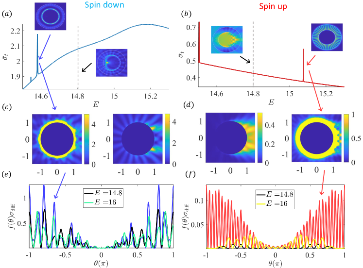
With the configuration in Fig. 1, the edge modes are relativistic quantum resonant states that confine the electrons to a quasi-1D region, where the resonant energy is about half of the potential. Figure 2(a) demonstrates an edge mode associated with spin-down electrons (the left inset) confined around $r^{\prime}\approx R_{2}$ with $E\approx 15=(V_{1}+V_{2})/2$ . For comparison, the right inset shows a conventional pseudospin-1 scattering mode [32]. Spin-up electrons, however, exhibit characteristically different scattering behaviors, as illustrated in Fig. 2(b) for two energy values. The corresponding scattering probability distributions for the spin-down and spin-up electrons are shown in Figs. 2(c) and 2(d), respectively. The edge mode produces a large scattering probability with wide directional distribution in both the near- and far-field regions. [Section IV.1 provides a detailed analysis of the edge-mode enhanced scattering for spin-down electrons.] In contrast, the scattering patterns for the spin-up electrons are reminiscent of lensing modes in geometric optics that arise in the small wavelength limit: $k_{\mathrm{II}}=|E-V_{1}|\approx 73$ , $k_{\mathrm{III}}=|E-V_{2}|\approx 23$ , and $k_{\mathrm{I}}=|E|\approx 15$ . The distinct scattering behaviors for spin-down and spin-up electrons can also be characterized by the momentum-transport cross section, defined as $\sigma_{tr}\equiv\oint d\theta f(\theta)\sigma_{\rm diff}$ with incident direction $\theta^{\prime}=0$ , where $f(\theta)\equiv 1-\cos\theta$ , the differential cross section $\sigma_{\rm diff}$ is determined by the scattering matrix, and $\sigma_{tr}$ is proportional to the resistance $\sigma^{\uparrow\downarrow}_{tr}\propto R^{\uparrow\downarrow}$ [details in Appendix C]. The edge modes generate a much larger resistance than the lensing states, as shown by the differential momentum-transport cross section in Figs. 2(e) and 2(f), respectively.

The physical reason underlying the emergence of the edge modes lies in the boundary condition for the three-component spinor stipulated by the generalized Dirac-Weyl equation for pseudospin-1 quasiparticles [44]. In particular, the radial or normal current density across the boundary of the scatterer must be continuous, but it is not necessary for the angular or tangent component of the current density to be continuous. In addition, the probability density needs not be continuous across the boundary. In fact, a larger difference in the probability density can arise if there is a significant imbalance in the first and third components of the spinor across the boundary. If the scattering potential redistributes the spinor wave-function components properly, there will be a significant increase in the probability density from the exterior to the interior of the scattering boundary, leading to strong boundary trapping of the quasiparticles inside the potential and thereby to robust edge modes. This phenomenon of boundary confinement is most pronounced when the Fermi energy of the particle is about half of the potential height - the Klein tunneling regime [44].

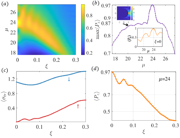
We now demonstrate that spin-dependent edge modes can lead to unusually nearly complete spin polarization. Figure 3(a) shows, in the 2D parameter plane ( $\xi,\mu)$ , color-coded values of the spin polarization averaged over a relevant range of the Fermi energy, which is defined as $\langle P_{z}\rangle=\langle(\sigma^{\downarrow}_{tr}-\sigma^{\uparrow}_{tr})/(\sigma^{\downarrow}_{tr}+\sigma^{\uparrow}_{tr})\rangle$ from Appendix C. There exists a relatively large area in the parameter plane in which the spin polarization exceeds $85\%$ . Figure 3(b) shows the maximum spin polarization versus $\mu$ , which can reach a value as high as $97\%$ (for $\mu\approx 24$ ), due to the drastically different scattering behaviors associated with the spin-down and spin-up electrons. Figure 3(c) shows, for $\mu=24$ , the energy-averaged momentum-transport cross sections $\langle\sigma_{tr}\rangle$ versus $\xi$ for spin-down and spin-up electrons, where the cross section values for spin-down electrons are markedly larger than those for spin-up electrons. The difference is the largest for $\xi\gtrsim 0$ , leading to the highest spin polarization there. For a fixed value of $\mu$ , as $\xi$ increases from zero (integrable classical dynamics) to, e.g., 0.3 (chaotic classical dynamics), the spin polarization can be maximized by some value of $\xi$ [details in Appendix E]. Figure 3(d) shows the average spin polarization versus $\xi$ for $\mu=24$ . Since $\xi$ is a geometric parameter “controlling” the degree of classical chaos (as $\xi$ increases from zero, the classical dynamics become more chaotic), the result shows that classical chaos deteriorates spin polarization.

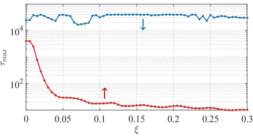
The characteristic difference between the edge modes for spin-down electrons and the lensing modes for spin-up electrons can also be revealed by the maximum Wigner-Smith time delay defined as $\tau(E)\equiv-i\hbar\mathrm{Tr}[S^{\dagger}\partial S/\partial E]$ , with $S$ being the scattering matrix in Appendix C. Figure 4 shows, for $\mu=24$ , the maximum delay $\tau_{max}$ (over Fermi energy) versus the geometric parameter $\xi$ for spin-down (blue) and spin-up (red) electrons, where the former is significantly larger than that for the latter. A remarkable feature is that, as $\xi$ increases from zero so that the classical dynamics changes from being integrable to mixed and then to chaotic, $\tau_{max}$ for spin-down electrons hardly vary, indicating that the edge modes have no classical correspondence. In contrast, $\tau_{max}$ for spin-up electrons continue to decrease with $\xi$ , which agrees with the classical intuition that, as the dynamics become more chaotic, the average time that an electron can stay inside the cavity should decrease. Because of the classical-quantum correspondence for the lensing modes, their properties can be understood using ray tracing from geometric optics in Appendix G.

IV Discussion

IV.1 Emergence of edge mode in the chaotic stadium cavity

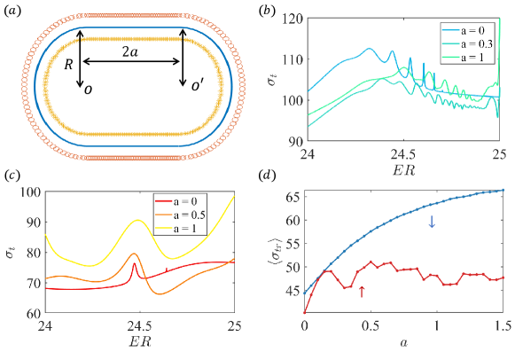
In a previous work [32], it was demonstrated that an edge mode can confine a particle for a long time, defying any Q-spoiling effect induced by classical chaos. To further demonstrate the “peculiar” behavior of the edge modes, we set up and study a spin-resolved scattering cavity of the stadium shape, whose geometric boundary is shown as the blue curve in Fig. 5(a), where $a$ is a so-called “chaotic parameter” in the sense that the classical dynamics are chaotic for $a>0$ . To calculate the scattering cross sections, we use a previously developed method, the multiple-multipole method [32], where two sets of “dipoles”, one inside and another outside the cavity, as shown in Fig. 5(a), are used as the sources to produce the far-field scattering wave function. For spin-down electrons, the total potential in the cavity is $V_{0}=50$ . There are quasibound edge modes with Fermi energy about half of the total potential, as shown by the peaks in the total cross section in Fig. 5(b). For spin-up electrons, the total potential in the cavity is $V_{0}=70$ and the classical dynamics are chaotic, which smooths out the sharp resonances, as shown in Fig. 5(c). For the edge mode associated with spin-down electrons, the resonant peaks have also been smoothed out. Intuitively, a larger potential in the cavity produces stronger scattering. However, the edge mode leads to strong scattering even with a small potential, as shown in Fig. 5(d), the momentum-transport cross section versus the stadium parameter $a$ . It can be seen that a spin-down electron, due to its large momentum-transport cross section $\langle\sigma_{tr}\rangle$ as the result of the edge mode, produces larger and larger equivalent scattering resistance than that from a spin-up electron as the chaotic parameter increases.

IV.2 Conclusion and outlook

We design the whole scatterer placed on a magnetic insulator substrate so that the real spin degree of the electrons matters in the sense that the spin-up and spin-down electrons will experience a different magnetic exchange potential. Based on this, we articulated a simple eccentric circular scatterer to generate edge modes for electrons with a specific spin orientation, where the electrons can be confined around the edge modes for a long time, generating resonant scattering with a large momentum-transport cross section. The quantum scattering behaviors for these electrons do not have a classical correspondence. On the contrary, electrons with the opposite spin will not possess such edge modes: they tend to stay in the scattering region for a much shorter time with a small cross section. For these electrons, the quantum scattering dynamics have a classical correspondence, so ray tracing with Dirac electron optics can be used to understand their behaviors (see Appendix G). The remarkable difference in the spin-specific scattering cross sections leads to tunable spin polarization and can even generate near-perfect spin polarization. The physical principles laid out in this work are anticipated to find applications in spintronics.

The basic principle of spintronics is to manipulate the spin degree of freedom to bring new capabilities to microelectronics and information technology with applications such as magnetic memories and sensors, radio-frequency and microwave devices, and logic and non-Boolean devices [45]. In spintronics, a key requirement is to achieve high spin polarization in functional materials [46], which has remained to be a challenge. For example, the early proposition of spin field-effect transistors for large-scale integrated circuits [47] requires high spin polarization [48, 49, 50, 46, 51, 52]. Graphene spintronics [53] based on relativistic quantum mechanics of pseudospin-1/2 fermions possess certain advantages such as room-temperature spin transport with long spin diffusion lengths of several micrometers [54, 55], gate-tunable carrier concentration, high electronic mobility, and efficient spin injection [56, 57]. However, even for graphene, designing a system configuration to achieve high spin polarization is challenging [2] but holds some breakthroughs. For instance, the work in [58] realizes 100% spin and valley polarized in monolayer transition metal dichalcogenides(TMD) assisted by total external reflection with spin-orbit coupling and electrostatic potential barrier. Another work [59] also realizes the nearly ±100% spin-polarized current by the magnetic configuration in two-terminal bipolar spin diodes of zigzag graphene nanoribbons. Although the artificial magnetic field in 2D materials can also produce spin polarization and other intriguing physical effects, it requires the systematical technology to employ and control the magnetic field, of which the magnitude is hard to achieve the order of tesla. Conversely, adding magnetic insulators [19, 20] or magnetic impurities [60] on top of 2D materials can induce the magnetic exchange field (MEF), which can potentially reach at least several tesla magnitudes [23, 19]. In addition, MEF facilitates extensive research on electronic optics [25, 26, 27, 28, 2, 29, 30, 31]. To summarize, it holds the fundamental and applicable interest to explore the physical nature of 2D materials with MEF interaction.

Experimentally, it has become feasible to implement electron scattering in 2D Dirac materials. For example, the width of p-n junction edge in Dirac materials can already be made sufficiently sharp [43, 27, 12] (e.g., $d\sim 1$ nm compared with the typical Fermi wavelength $\lambda_{F}\sim 10$ nm). In addition, the materials can be fabricated on the scale of micrometers to reach the small wavelength limit at which Dirac electron optics is applicable [61]. The required magnetic exchange potential has been realized in experiments [19, 20]. For electrostatic potential in the eccentric circular shape, in the recent experiment [13], a circular p-n junction, i.e. a local embedded gate, in a graphene/hBN heterostructure is created by local defect charge and STM tip with a square voltage pulse. Moreover, the Dirac electron scattering in the multi-circular quantum dots has been discussed [14]. It implies the possibility of fabrication of the eccentric circular cavity shape by STM technology. Experimental material platforms have also existed to create pseudospin-1 Dirac systems with a flat band, such as the transition-metal oxide $\mbox{SrTiO}_{3}/\mbox{SrIrO}_{3}/\mbox{SrTiO}_{3}$ trilayer heterostructures [62], $\mbox{SrCu}_{2}(\mbox{BO}_{3})_{2}$ [63], and graphene- $\mbox{In}_{2}\mbox{Te}_{2}$ bilayer [64].

Acknowledgment

This work was supported by AFOSR under Grant No. FA9550-21-1-0186.

Appendix A S-Matrix approach to elastic Dirac electron scattering

Consider electronic scattering from a cavity made of two-dimensional (2D) Dirac materials with a flat band. At low energies, the effective Hamiltonian describes the dynamics of a pseudospin-1 Dirac-Weyl quasiparticle. The cavity is subject to external electrical and magnetic exchange fields: its properties are controlled by an electric gate potential $\mathcal{V}_{gate}(\mathbf{r})$ and a magnetic exchange potential $\mathcal{M}(\mathbf{r})$ induced by the magnetic insulator substrate within the gate region [2]. The total Hamiltonian is

	$\displaystyle\hat{H}=v_{F}\sigma_{0}\otimes\mathbf{S}\cdot\mathbf{\hat{p}}+\hbar v_{F}[\sigma_{0}\otimes$	$\displaystyle S_{0}\mathcal{V}_{gate}(\mathbf{r})$
		$\displaystyle-\sigma_{z}\otimes S_{0}\mathcal{M}(\mathbf{r})],$		(5)

where $\mathbf{S}$ denotes the vector of spin-1 matrices, $\sigma_{0}$ and $S_{0}$ are the two-by-two and three-by-three identity matrices, respectively, $\sigma_{z}$ is the Pauli $z$ matrix, and $v_{F}$ is the Fermi velocity. Tensor product of the three-component pseudospin-1 quasiparticles and two-component real spin $1/2$ electron, so the Hamiltonian matrix is six-by-six, which can be block-diagonalized as $\hat{H}={\rm diag}[\hat{H}_{1},\hat{H}_{-1}]$ with the following two three-by-three sub-Hamiltonian matrices $\hat{H}_{s}$ for real spin index $s=\pm 1$ :

\displaystyle\hat{H}_{s}=v_{F}\mathbf{S}\cdot\mathbf{\hat{p}}+\hbar v_{F}[\mathcal{V}_{gate}(\mathbf{r})-s\mathcal{M}(\mathbf{r})],

(6)

where the identity $[\sigma_{z}\otimes S_{0},\hat{H}]=0$ has been used. The total potential is spin-dependent:

\displaystyle V^{s}(\mathbf{r})\equiv\mathcal{V}_{gate}(\mathbf{r})-s\mathcal{M}(\mathbf{r}).

The prototypical system we use to demonstrate achieving high spin polarization is an eccentric circular cavity defined by two distinct radii: $R_{1}$ and $R_{2}<R_{1}$ , where the centers of the two circles are located at $O$ (the larger disk) and $O^{\prime}$ (the smaller disk) with the eccentric distance $\xi$ between $OO^{\prime}$ , as shown in Fig. 1(b) in the main text. For convenience, we define three regions in the position space: region $\mathrm{I}$ with $V_{0}=0$ for $r>R_{1}$ , region $\mathrm{II}$ with $V^{s}_{1}$ for $r<R_{1}$ and $r^{\prime}>R_{2}$ , and region $\mathrm{III}$ with $V^{s}_{2}$ for $r^{\prime}<R_{2}$ . The wave vectors in the three regions are given by

	$\displaystyle k_{\mathrm{I}}$	$\displaystyle=\|E\|,$
	$\displaystyle k^{s}_{\mathrm{II}}$	$\displaystyle=\|E-V^{s}_{\mathrm{1}}\|,$
	$\displaystyle k^{s}_{\mathrm{III}}$	$\displaystyle=\|E-V^{s}_{\mathrm{2}}\|.$

The wave functions in the three regions can be written down according to the standard form of the spinor wave eigenvector of $\hat{H}_{s}$ in the cylindrical coordinates, which are given by

\displaystyle^{k}g_{m}=\frac{1}{\sqrt{2}}\left(\begin{array}[]{c}f_{m-1}(kr)e^{-i\theta}\\ i\alpha\sqrt{2}f_{m}(kr)\\ -f_{m+1}(kr)e^{i\theta}\end{array}\right)e^{im\theta},

(10)

where $\alpha\equiv\mathrm{sign}(E-V)$ , $k=|E-V|$ . There are two cases for the function $f_{m}(kr)$ : (i) $f_{m}=H^{(1,2)}_{m}$ , the Hankel functions of the first and the second kind, and (ii) $f_{m}=J_{m}$ , the Bessel function. For cases (i) and (ii), ${}^{k}g_{m}$ is given by ${{}^{k}g_{m}}={{}^{k}h^{(1,2)}_{m}}$ and ${{}^{k}g_{m}}={{}^{k}j_{m}}$ , respectively. In particular, in region $\mathrm{I}$ , the wave function can be expanded in the spinor cylindrical wave basis as

\displaystyle\Psi^{(\mathrm{I})}(\vec{r})=\sum_{m=-\infty}^{+\infty}a^{\mathrm{I}}_{m}\left[{{}^{k_{\mathrm{I}}}h^{(2)}_{m}}+\sum_{j=-\infty}^{+\infty}S_{mj}\;{{}^{k_{\mathrm{I}}}h^{(1)}_{j}}\right].

(11)

In region II, the wave function can be written as

\displaystyle\Psi^{(\mathrm{II})}(\vec{r})=\sum_{m=-\infty}^{+\infty}\sum_{l=-\infty}^{+\infty}{{}^{m}}a^{\mathrm{II}}_{l}\left[{{}^{k_{\mathrm{II}}}h^{(2)}_{l}}+\sum_{j=-\infty}^{+\infty}S^{od}_{lj}\;{{}^{k_{\mathrm{II}}}h^{(1)}_{j}}\right],

(12)

where $S^{od}$ is the off-diagonal scattering matrix for the eccentric circular cavity and $S^{cd}$ is the diagonal matrix to characterize the scattering from a circular domain [2], which are related by $S^{od}=U^{-1}S^{cd}U$ , or

	$\displaystyle S^{od}_{lj}$	$\displaystyle=\sum_{l^{\prime},j^{\prime}}(U^{-1})_{ll^{\prime}}S^{cd}_{l^{\prime}j^{\prime}}U_{j^{\prime}j}$
		$\displaystyle=\sum_{l^{\prime},j^{\prime}}J_{l-l^{\prime}}(k_{\mathrm{II}}\xi)S^{cd}_{l^{\prime}l^{\prime}}\delta_{l^{\prime}j^{\prime}}J_{j-j^{\prime}}(k_{\mathrm{II}}\xi)$
		$\displaystyle=\sum_{l^{\prime}}J_{l-l^{\prime}}S^{cd}_{l^{\prime}l^{\prime}}J_{j-l^{\prime}}.$

The boundary conditions for a pseudospin-1 quasiparticle [44] stipulate continuity of the second component of the spinor wave function and conservation of the radial current density:

	$\displaystyle\Psi^{\mathrm{I}}_{2}(R_{1})$	$\displaystyle=\Psi^{\mathrm{II}}_{2}(R_{1}),$		(13)
	$\displaystyle\Psi^{\mathrm{I}}_{1}(R_{1})e^{i\theta}+\Psi^{\mathrm{I}}_{3}(R_{1})e^{-i\theta}$	$\displaystyle=\Psi^{\mathrm{II}}_{1}(R_{1})e^{i\theta}+\Psi^{\mathrm{II}}_{3}(R_{1})e^{-i\theta}.$		(14)

	$\displaystyle\Psi^{\mathrm{I}}_{1}(R_{1})$	$\displaystyle=\Psi^{\mathrm{II}}_{1}(R_{1}),$
	$\displaystyle\Psi^{\mathrm{I}}_{2}(R_{1})$	$\displaystyle=\Psi^{\mathrm{II}}_{2}(R_{1}).$

In matrix form, the boundary conditions can be expressed as

$\displaystyle A^{\mathrm{I}}[X^{(2)}+SX^{(1)}]$	$\displaystyle=\alpha_{\mathrm{I}}\alpha_{\mathrm{II}}A^{\mathrm{II}}[x^{(2)}+S^{od}x^{(1)}],$	(15)
$\displaystyle A^{\mathrm{I}}[[Z^{(2)}-Y^{(2)}]$	$\displaystyle+S[Z^{(1)}-Y^{(1)}]]$	(16)
	$\displaystyle=A^{\mathrm{II}}[[z^{(2)}-y^{(2)}]+S^{od}[z^{(1)}-y^{(1)}]],$

where $\alpha_{\mathrm{I}}\equiv\mathrm{sign}(E)$ , $\alpha_{\mathrm{II}}\equiv\mathrm{sign}(E-V_{1})$ , $A^{\mathrm{I}}\equiv[a^{\mathrm{I}}_{m}\delta_{mj}]$ , $A^{\mathrm{II}}\equiv[{{}^{m}}a^{\mathrm{II}}_{j}]$ and

$\displaystyle X^{(1,2)}$	$\displaystyle\equiv[H^{(1,2)}_{m}(k_{\mathrm{I}}R_{1})\delta_{mj}],\;x^{(1,2)}\equiv[H^{(1,2)}_{m}(k_{\mathrm{II}}R_{1})\delta_{mj}];$
$\displaystyle Y^{(1,2)}$	$\displaystyle\equiv[H^{(1,2)}_{m+1}(k_{\mathrm{I}}R_{1})\delta_{mj}],\;y^{(1,2)}\equiv[H^{(1,2)}_{m+1}(k_{\mathrm{II}}R_{1})\delta_{mj}];$
$\displaystyle Z^{(1,2)}$	$\displaystyle\equiv[H^{(1,2)}_{m-1}(k_{\mathrm{I}}R_{1})\delta_{mj}],\;z^{(1,2)}\equiv[H^{(1,2)}_{m-1}(k_{\mathrm{II}}R_{1})\delta_{mj}].$	(17)

The spinor wave function can be written as

{}^{k}h_{m}^{(1,2)}=\frac{1}{\sqrt{2}}\left(\begin{array}[]{c}H^{(1,2)}_{m-1}(kr)e^{-i\theta}\\ i\alpha\sqrt{2}H^{(1,2)}_{m}(kr)\\ -H^{(1,2)}_{m+1}(kr)e^{i\theta}\end{array}\right)e^{im\theta},

(21)

where the general form of the basis is described by Eq. (10). The scattering matrix can be written as

S=-\frac{Z^{(2)}-Y^{(2)}-\alpha_{\mathrm{I}}\alpha_{\mathrm{II}}X^{(2)}\mathcal{T}}{Z^{(1)}-Y^{(1)}-\alpha_{\mathrm{I}}\alpha_{\mathrm{II}}X^{(1)}\mathcal{T}},

(22)

where $\mathcal{T}\equiv F^{-1}[H-G]$ , and

$\displaystyle F$	$\displaystyle\equiv x^{(2)}+S^{od}x^{(1)},$
$\displaystyle G$	$\displaystyle\equiv y^{(2)}+S^{od}y^{(1)},$
$\displaystyle H$	$\displaystyle\equiv z^{(2)}+S^{od}z^{(1)}.$	(23)

The coefficient $A^{\mathrm{I}}$ is determined by the incident wave function (see Appendix C), and the coefficient $A^{\mathrm{II}}$ is given by

\displaystyle A^{\mathrm{II}}=\alpha_{\mathrm{I}}\alpha_{\mathrm{II}}A^{\mathrm{I}}[X^{(2)}+SX^{(1)}]F^{-1}.

Using the Graf’s addition theorem [14], we have, for $r^{\prime}>\xi$ ,

H^{(1,2)}_{m}(kr)e^{im\theta}=\sum_{n=-\infty}^{+\infty}J_{m-n}(k\xi)e^{in\theta^{\prime}}H^{(1,2)}_{n}(kr^{\prime}),

(24)

which gives

{{}^{k}}h_{m}^{(1,2)}=\sum_{n=-\infty}^{+\infty}J_{m-n}(k\xi)\;{{}^{k}}\widetilde{h}_{n}^{(1,2)}.

(25)

For convenience, in the following, we use the tilde symbol to denote the quantities in the circular region of origin at $O^{\prime}$ . We have

$\displaystyle{{}^{k_{\mathrm{II}}}h^{(2)}_{l}}+\sum_{j=-\infty}^{+\infty}S^{od}_{lj}\;{{}^{k_{\mathrm{II}}}h^{(1)}_{j}}$	$\displaystyle=\sum_{n=-\infty}^{+\infty}J_{l-n}(k_{\mathrm{II}}\xi)\;{{}^{k_{\mathrm{II}}}}\widetilde{h}^{(2)}_{n}+\sum_{j=-\infty}^{+\infty}S^{od}_{lj}\left[\sum_{n=-\infty}^{+\infty}J_{j-n}(k_{\mathrm{II}}\xi)\;{{}^{k_{\mathrm{II}}}}\widetilde{h}^{(1)}_{n}\right]$
	$\displaystyle=\sum_{l^{\prime}=-\infty}^{+\infty}J_{l-l^{\prime}}\;{{}^{k_{\mathrm{II}}}}\widetilde{h}^{(2)}_{l^{\prime}}+\sum_{n,l^{\prime}=-\infty}^{+\infty}J_{l-l^{\prime}}S^{cd}_{l^{\prime}l^{\prime}}\sum_{j=-\infty}^{+\infty}(J_{j-l^{\prime}}J_{j-n})\;{{}^{k_{\mathrm{II}}}}\widetilde{h}^{(1)}_{n}$
	$\displaystyle=\sum_{l^{\prime}=-\infty}^{+\infty}J_{l-l^{\prime}}(k_{\mathrm{II}}\xi)\left[{{}^{k_{\mathrm{II}}}\widetilde{h}^{(2)}_{l^{\prime}}}+S^{cd}_{l^{\prime}l^{\prime}}\;{{}^{k_{\mathrm{II}}}\widetilde{h}^{(1)}_{l^{\prime}}}\right],$	(26)

where

\displaystyle\delta_{l^{\prime}n}=\sum_{j=-\infty}^{+\infty}J_{j-l^{\prime}}(k_{\mathrm{II}}\xi)J_{j-n}(k_{\mathrm{II}}\xi).

The wave function in region $\mathrm{II}$ with origin $O$ can be rewritten as a wave function with origin $O^{\prime}$ as $\Psi^{\mathrm{II}}(r,\theta)=\widetilde{\Psi}^{\mathrm{II}}(r^{\prime},\theta^{\prime})$ , where

\displaystyle\widetilde{\Psi}^{\mathrm{II}}(r^{\prime},\theta^{\prime})=\sum_{m=-\infty}^{+\infty}\sum_{l=-\infty}^{+\infty}{{}^{m}}\widetilde{a}^{\mathrm{II}}_{l}\left[{{}^{k_{\mathrm{II}}}}\widetilde{h}^{(2)}_{l}+S^{cd}_{ll}\;{{}^{k_{\mathrm{II}}}}\widetilde{h}^{(1)}_{l}\right],

with ${{}^{m}}\widetilde{a}^{\mathrm{II}}_{l}\equiv\sum_{l^{\prime}}{{}^{m}}a^{\mathrm{II}}_{l^{\prime}}J_{l^{\prime}-l}(k_{\mathrm{II}}\xi)$ . In region $\mathrm{III}$ with origin $O^{\prime}$ , the wavefunction is given by

\widetilde{\Psi}^{\mathrm{III}}(r^{\prime},\theta^{\prime})=\sum_{m=-\infty}^{+\infty}\sum_{l=-\infty}^{+\infty}{{}^{m}}\widetilde{b}_{l}\;{{}^{k_{\mathrm{III}}}}\widetilde{j}_{l}.

(27)

Using the boundary condition Eq. (13), we obtain

{{}^{m}}\widetilde{b}_{l}=\alpha_{\mathrm{II}}\alpha_{\mathrm{III}}{{}^{m}}\widetilde{a}^{\mathrm{II}}_{l}\;\frac{H^{(2)}_{l}(k_{\mathrm{II}}R_{2})+S^{cd}_{ll}H^{(1)}_{l}(k_{\mathrm{II}}R_{2})}{J_{l}(k_{\mathrm{III}}R_{2})}.

(28)

Appendix B Scattering matrix for a circular cavity

To obtain the scattering matrix $S^{cd}$ , we consider a circular cavity of radius $R_{2}$ centered at $O$ where $r>R_{2}$ and $0<r<R_{2}$ define regions $\mathrm{II}$ and $\mathrm{III}$ , respectively. Due to the circular symmetry, the wave function for each angular momentum channel can be written as

	$\displaystyle\Psi^{\mathrm{II}}_{m}$	$\displaystyle={{}^{k_{\mathrm{II}}}}h^{(2)}_{m}+S^{cd}_{mm}\;{{}^{k_{\mathrm{II}}}}h^{(1)}_{m}$
	$\displaystyle\Psi^{\mathrm{III}}_{m}$	$\displaystyle=B_{m}{{}^{k_{\mathrm{III}}}}j_{m}.$		(29)

Applying the boundary conditions gives

	$\displaystyle\alpha_{\mathrm{II}}\left[H^{(2)}_{m}(k_{\mathrm{II}}R_{2})+S^{cd}_{mm}H^{(1)}_{m}(k_{\mathrm{II}}R_{2})\right]$	$\displaystyle=\alpha_{\mathrm{III}}B_{m}J_{m}(k_{\mathrm{III}}R_{2})$
	$\displaystyle{{}^{k_{\mathrm{II}}}_{1+3}}h^{(2)}_{m}(R_{2})+S^{cd}_{mm}\leavevmode\nobreak\ {{}^{k_{\mathrm{II}}}_{1+3}}h^{(1)}_{m}(R_{2})$	$\displaystyle=B_{m}\leavevmode\nobreak\ {{}^{k_{\mathrm{III}}}_{1+3}}j_{m}(R_{2}),$		(30)

where

	$\displaystyle{{}^{k_{\mathrm{II}}}_{1+3}}h^{(1,2)}_{m}(R_{2})$	$\displaystyle\equiv H^{(1,2)}_{m-1}(k_{\mathrm{II}}R_{2})-H^{(1,2)}_{m+1}(k_{\mathrm{II}}R_{2})$		(31)
	$\displaystyle{{}^{k_{\mathrm{III}}}_{1+3}}j_{m}(R_{2})$	$\displaystyle\equiv J_{m-1}(k_{\mathrm{III}}R_{2})-J_{m+1}(k_{\mathrm{III}}R_{2}).$		(32)

We thus have

S^{cd}_{mm}=-\frac{J_{m}(k_{\mathrm{III}}R_{2})\leavevmode\nobreak\ {{}^{k_{\mathrm{II}}}_{1+3}}h^{(2)}_{m}(R_{2})-\alpha_{\mathrm{II}}\alpha_{\mathrm{III}}H^{(2)}_{m}(k_{\mathrm{II}}R_{2})\leavevmode\nobreak\ {{}^{k_{\mathrm{III}}}_{1+3}}j_{m}(R_{2})}{J_{m}(k_{\mathrm{III}}R_{2})\leavevmode\nobreak\ {{}^{k_{\mathrm{II}}}_{1+3}}h^{(1)}_{m}(R_{2})-\alpha_{\mathrm{II}}\alpha_{\mathrm{III}}H^{(1)}_{m}(k_{\mathrm{II}}R_{2})\leavevmode\nobreak\ {{}^{k_{\mathrm{III}}}_{1+3}}j_{m}(R_{2})}\leavevmode\nobreak\ ,

(33)

with $\alpha_{\mathrm{III}}\equiv\mathrm{sign}(E-V_{2})$ .

Appendix C Scattering cross sections

The wave function in region $\mathrm{I}$ from Eq. (11) can be rewritten as the sum of the contributions from the incident and scattering waves:

	$\displaystyle\Psi^{(\mathrm{I})}(\vec{r})$	$\displaystyle=\sum_{m=-\infty}^{\infty}a^{\mathrm{I}}_{m}\left[2\;{{}^{k_{\mathrm{I}}}j_{m}}+\sum_{m^{\prime}=-\infty}^{\infty}(S_{mm^{\prime}}-\delta_{mm^{\prime}}){{}^{k_{\mathrm{I}}}h^{(1)}_{m^{\prime}}}\right]$
		$\displaystyle=\chi_{in}+\sum_{m=-\infty}^{\infty}a^{\mathrm{I}}_{m}\sum_{m^{\prime}=-\infty}^{\infty}T_{mm^{\prime}}\leavevmode\nobreak\ {{}^{k_{\mathrm{I}}}h^{(1)}_{m^{\prime}}}.$		(34)

The incident wave function corresponds to

\displaystyle\chi_{in}\equiv\sum_{m=-\infty}^{\infty}2a^{\mathrm{I}}_{m}{{}^{k_{\mathrm{I}}}j_{m}}.

(35)

The norm square of the second term in Eq. (C), which is the scattering wave function, is defined as the scattering probability in the near field measured from the cavity in region $\mathrm{I}$ , with the transmission matrix defined as $T_{mm^{\prime}}\equiv S_{mm^{\prime}}-\delta_{mm^{\prime}}$ . The coefficient $a^{\mathrm{I}}_{m}$ for each angular momentum channel is determined by the incident plane wave function:

\displaystyle\chi_{in}(r,\theta)

\displaystyle=\frac{1}{2}\left(\begin{array}[]{c}e^{-i\theta^{\prime}}\\ \sqrt{2}s\\ e^{i\theta^{\prime}}\end{array}\right)e^{i\mathbf{k}_{in}\cdot\mathbf{r}},

(39)

with the incident wave vector $\mathbf{k}_{in}=k_{\mathrm{I}}(\cos\theta^{\prime},\sin\theta^{\prime})$ . Expanding the incident wave function for each angular momentum channel by the Jacobi-Anger formula

e^{ik_{\mathrm{I}}r\cos(\theta-\theta^{\prime})}=\sum_{m=-\infty}^{+\infty}i^{m}J_{m}(k_{\mathrm{I}}r)e^{im(\theta-\theta^{\prime})},

(40)

we obtain

\chi_{in}(r,\theta)=\sum_{m=-\infty}^{+\infty}\frac{1}{\sqrt{2}}\;i^{m-1}e^{-im\theta^{\prime}}\;{{}^{k_{\mathrm{I}}}}j_{m}.

(41)

Note that $j_{m}$ is the three components vector defined by Eq. (10) while $J_{m}$ is the scalar Bessel function. The coefficient $a^{\mathrm{I}}_{m}(\theta^{\prime})$ in Eq. (C) and Eq. (35) is then given by

\displaystyle a^{\mathrm{I}}_{m}(\theta^{\prime})=i^{m-1}e^{-im\theta^{\prime}}/(2\sqrt{2}).

(42)

Scattering cross section characterizes the behavior of particles in the far-field region $kr\gg 1$ (from the cavity). In the far field, the wave function from Eq. (C) tends to

\lim_{kr\gg 1}\psi(r,\theta)=\chi_{in}+\frac{f(\theta,\theta^{\prime})}{2\sqrt{-ir}}\left(\begin{array}[]{c}e^{-i\theta}\\ \sqrt{2}s\\ e^{i\theta}\end{array}\right)e^{ik_{\mathrm{I}}r}

(43)

with the scattering angle distribution in the far field as

\displaystyle f(\theta,\theta^{\prime})=\frac{2}{\sqrt{\pi k_{\mathrm{I}}}}\sum_{m=-\infty}^{\infty}a_{m}^{\mathrm{I}}(\theta^{\prime})\sum_{m^{\prime}=-\infty}^{\infty}T_{mm^{\prime}}(-i)^{m^{\prime}}e^{im^{\prime}\theta},

(44)

a result of the asymptotic behavior of the Hankel function:

\displaystyle\lim_{x\rightarrow{}\infty}H^{(1,2)}_{m}(x)\rightarrow\sqrt{\frac{2}{\pi x}}e^{\pm i(x-m\pi/2-\pi/4)},

and the standard plane-wave normalization requirement. The differential cross section $\sigma_{\rm diff}$ is given in terms of $f(\theta,\theta^{\prime})$ as

\sigma_{\rm diff}\equiv\frac{d\sigma}{d\theta}=|f(\theta,\theta^{\prime})|^{2},

(45)

and the total scattering cross section, which records the probability of scattering events under all possible directions, is given by

\sigma_{t}(\theta^{\prime})=\oint d\theta|f(\theta,\theta^{\prime})|^{2}.

(46)

The momentum-transport cross section is defined as

\sigma_{tr}(\theta^{\prime})=\oint d\theta(1-\cos\theta)|f(\theta,\theta^{\prime})|^{2}.

(47)

Averaging over the incident angle $\theta^{\prime}$ leads to

	$\displaystyle\bar{\sigma}_{t}=\frac{1}{2\pi}\oint d\theta^{\prime}\sigma_{t}(\theta^{\prime}),$		(48)
	$\displaystyle\bar{\sigma}_{tr}=\frac{1}{2\pi}\oint d\theta^{\prime}\sigma_{tr}(\theta^{\prime}).$		(49)

Performing an average over some Fermi energy interval, we get

\displaystyle\langle\sigma_{tr}\rangle=\frac{1}{E_{1}-E_{0}}\int^{E_{1}}_{E_{0}}dE\leavevmode\nobreak\ \sigma_{tr}(E).

(50)

The momentum transport cross section determines the transport relaxation time $\tau_{tr}$ through

\frac{1}{\tau_{tr}}=n_{c}v_{F}\sigma_{tr},

(51)

where $n_{c}$ is the concentration of identical scatters. Our scattering system is sufficiently dilute so that multiple scattering events can be neglected. For ballistic transport and elastic scattering with system size comparable with the mean free path: $\mathcal{L}_{s}\approx\mathcal{L}_{\rm mean-free}=v_{F}\tau_{tr}$ , the semiclassical Boltzmann transport theory gives that the conductivity is inverse of the $\sigma_{tr}$ :

G\propto\frac{1}{\sigma_{tr}}.

(52)

The spin polarization is defined by the spin-resolved transmission coefficient as [65]

\displaystyle P_{z}=(T^{\downarrow}-T^{\uparrow})/(T^{\downarrow}+T^{\uparrow}).

We thus have

P_{z}=\frac{\sigma_{tr}^{\downarrow}-\sigma_{tr}^{\uparrow}}{\sigma_{tr}^{\downarrow}+\sigma_{tr}^{\uparrow}},

(53)

with $\sigma^{\downarrow\uparrow}_{tr}\propto R^{\downarrow\uparrow}$ , where the resistance R is the inverse of the conductivity $G$ .

Appendix D Validation of S-matrix approach

D.1 Reduction from eccentric circular to annular cavity

For an annular scattering cavity ( $\xi=0$ ), the scattering matrix can be analytically calculated, providing a way to validate the scattering-matrix approach to the general case of $\xi\neq 0$ . For this purpose, we consider the annular scattering cavity $\xi=0$ but with two boundaries: one at $R_{1}$ and another at $R_{2}$ . In the three regions, the wave functions associated with an angular momentum channel are

$\displaystyle\Psi^{\mathrm{I}}_{m}$	$\displaystyle={{}^{k_{\mathrm{I}}}}h^{(2)}_{m}+S_{mm}\leavevmode\nobreak\ {{}^{k_{\mathrm{I}}}}h^{(1)}_{m},$
$\displaystyle\Psi^{\mathrm{II}}_{m}$	$\displaystyle=A_{m}[{{}^{k_{\mathrm{II}}}}h^{(2)}_{m}+S^{cd}_{mm}\leavevmode\nobreak\ {{}^{k_{\mathrm{II}}}}h^{(1)}_{m}],$
$\displaystyle\Psi^{\mathrm{III}}_{m}$	$\displaystyle=B_{m}{{}^{k_{\mathrm{III}}}}j_{m}.$	(54)

Imposing the boundary conditions at $r=R_{1}$ and $r=R_{2}$ gives

\displaystyle\left[\begin{array}[]{cccc}{{}^{k_{\mathrm{II}}}_{2}}h^{(2)}_{m}(R_{1})&0&{{}^{k_{\mathrm{II}}}_{2}}h^{(1)}_{m}(R_{1})&-{{}^{k_{\mathrm{I}}}_{2}}h^{(1)}_{m}(R_{1})\\ {{}^{k_{\mathrm{II}}}_{1+3}}h^{(2)}_{m}(R_{1})&0&{{}^{k_{\mathrm{II}}}_{1+3}}h^{(1)}_{m}(R_{1})&-{{}^{k_{\mathrm{I}}}_{1+3}}h^{(1)}_{m}(R_{1})\\ {{}^{k_{\mathrm{II}}}_{2}}h^{(2)}_{m}(R_{2})&-{{}^{k_{\mathrm{III}}}_{2}}j_{m}(R_{2})&{{}^{k_{\mathrm{II}}}_{2}}h^{(1)}_{m}(R_{2})&0\\ {{}^{k_{\mathrm{II}}}_{1+3}}h^{(2)}_{m}(R_{2})&-{{}^{k_{\mathrm{III}}}_{1+3}}j_{m}(R_{2})&{{}^{k_{\mathrm{II}}}_{1+3}}h^{(1)}_{m}(R_{2})&0\end{array}\right]\left[\begin{array}[]{c}A_{m}\\ B_{m}\\ C_{m}\\ S_{m}\end{array}\right]=\left[\begin{array}[]{c}{{}^{k_{\mathrm{I}}}_{2}}h^{(2)}_{m}(R_{1})\\ {{}^{k_{\mathrm{I}}}_{1+3}}h^{(2)}_{m}(R_{1})\\ 0\\ 0\end{array}\right],

(67)

where $C_{m}\equiv A_{m}S^{cd}_{mm}$ and

	$\displaystyle{{}^{k_{i}}_{2}}h^{(1,2)}_{m}(R_{j})$	$\displaystyle=s_{i}H^{(1,2)}_{m}(k_{i}R_{j}),$
	$\displaystyle{{}^{k_{i}}_{1+3}}h^{(1,2)}_{m}(R_{j})$	$\displaystyle=H^{(1,2)}_{m-1}(k_{i}R_{j})-H^{(1,2)}_{m+1}(k_{i}R_{j}),$
	$\displaystyle{{}^{k_{i}}_{2}}j_{m}(R_{j})$	$\displaystyle=s_{i}J_{m}(k_{i}R_{j}),$
	$\displaystyle{{}^{k_{i}}_{1+3}}j_{m}(R_{j})$	$\displaystyle=J_{m-1}(k_{i}R_{j})-J_{m+1}(k_{i}R_{j})$

with $i=\mathrm{I},\mathrm{II},\mathrm{III}$ and $j=1,2$ . Note that ${{}^{k_{\mathrm{II}}}_{2}}h^{(2)}_{m}(R_{1})$ and ${{}^{k_{\mathrm{II}}}_{1+3}}h^{(2)}_{m}(R_{1})$ are scalars, roughly corresponding to the second component and the sum of the first and third components of the radial part of ${{}^{k_{\mathrm{II}}}}h^{(2)}_{m}(R_{1})$ , respectively. We have

	$\displaystyle A_{m}$	$\displaystyle=\frac{s_{\mathrm{I}}H^{(2)}_{m}(k_{\mathrm{I}}R_{1})+s_{\mathrm{I}}H^{(1)}_{m}(k_{\mathrm{I}}R_{1})S_{mm}}{s_{\mathrm{II}}H^{(2)}_{m}(k_{\mathrm{II}}R_{1})+s_{\mathrm{II}}H^{(1)}_{m}(k_{\mathrm{II}}R_{1})S^{cd}_{mm}},$		(68)
	$\displaystyle B_{m}$	$\displaystyle=A_{m}\frac{s_{\mathrm{II}}H^{(2)}_{m}(k_{\mathrm{II}}R_{2})+s_{\mathrm{II}}H^{(1)}_{m}(k_{\mathrm{II}}R_{2})S^{cd}_{mm}}{s_{\mathrm{III}}J_{m}(k_{\mathrm{III}}R_{2})}.$		(69)

The scattering matrix is given by

S_{mm}=-\frac{s_{\mathrm{I}}y_{m}H^{(2)}_{m}(k_{\mathrm{I}}R_{1})-s_{\mathrm{II}}x_{m}[H^{(2)}_{m-1}(k_{\mathrm{I}}R_{1})-H^{(2)}_{m+1}(k_{\mathrm{I}}R_{1})]}{s_{\mathrm{I}}y_{m}H^{(1)}_{m}(k_{\mathrm{I}}R_{1})-s_{\mathrm{II}}x_{m}[H^{(1)}_{m-1}(k_{\mathrm{I}}R_{1})-H^{(1)}_{m+1}(k_{\mathrm{I}}R_{1})]},

(70)

where

	$\displaystyle x_{m}$	$\displaystyle=H^{(2)}_{m}(k_{\mathrm{II}}R_{1})+H^{(1)}_{m}(k_{\mathrm{II}}R_{1})S^{cd}_{mm}$
	$\displaystyle y_{m}$	$\displaystyle=[H^{(2)}_{m-1}(k_{\mathrm{II}}R_{1})-H^{(2)}_{m+1}(k_{\mathrm{II}}R_{1})]+[H^{(1)}_{m-1}(k_{\mathrm{II}}R_{1})-H^{(1)}_{m+1}(k_{\mathrm{II}}R_{1})]S^{cd}_{mm}.$

For the eccentric circular cavity, the scattering matrix can be determined by Eq. (22). We can reduce the eccentric cavity to an annular cavity by taking the limit $\xi\rightarrow 0$ . In that case, the off-diagonal scattering matrix will reduce to the diagonal matrix: $S^{od}_{lj}\rightarrow S^{cd}_{ll}\delta_{jl}$ and $S_{mm^{\prime}}\rightarrow S_{mm}\delta_{mm^{\prime}}$ . We have that Eq. (22) reduces to the same form of Eq. (70) as

S_{mm}=-\frac{Z^{(2)}_{m}-Y^{(2)}_{m}-s_{\mathrm{I}}s_{\mathrm{II}}X^{(2)}_{m}\mathcal{T}_{m}}{Z^{(1)}_{m}-Y^{(1)}_{m}-s_{\mathrm{I}}s_{\mathrm{II}}X^{(1)}_{m}\mathcal{T}_{m}}

(71)

with $\mathcal{T}_{m}=y_{m}/x_{m}$ . We find that, numerically, the difference between the scattering matrix in Eq. (71) and that in Eq. (70) is on the order of computer round-off error (about $10^{-15}$ ). The excellent agreement between the analytic S-matrix for $\xi=0$ and the numerically calculated matrix in the limit $\xi\rightarrow 0$ validates the S-matrix approach manifested through Eq. (22).

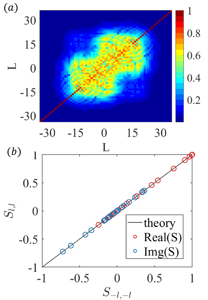
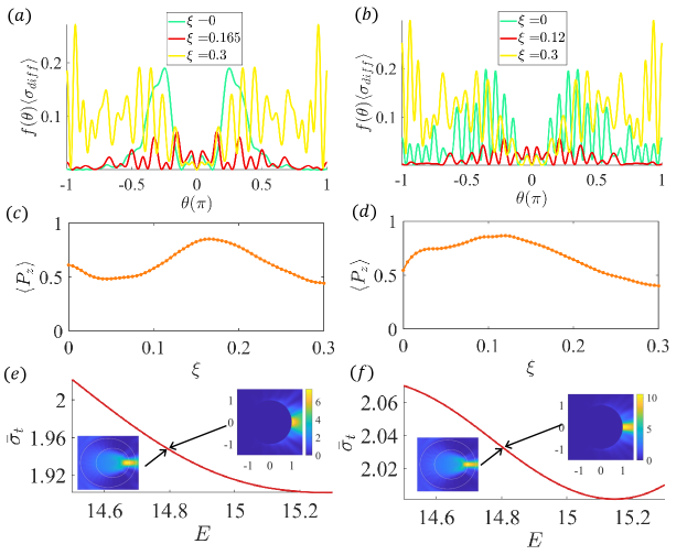
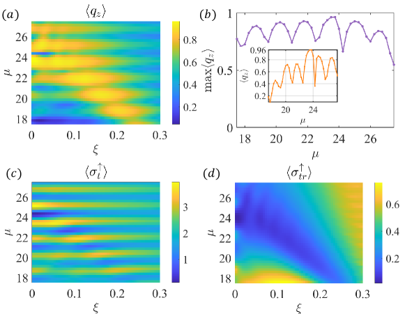
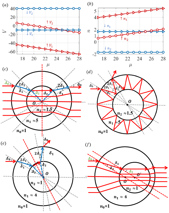
Figure 6(a) shows the convergence of the S-matrix in a large angular momentum range. For large angular momenta, the S-matrix elements are negligibly small, suggesting that these angular-momentum channels contribute little to the scattering process. More specifically, Fig. 6(a) is the color map of the S-matrix elements in the angular momentum representation. The near-zero components in the high angular momentum basis mean convergence. Note that the diagonal term in Fig. 6(a) will be removed in the transmission matrix $\mathcal{T}=S-I$ , which determines the scattering cross sections.

D.2 Mirror Symmetry

An eccentric circular cavity possesses the mirror (parity) symmetry. The parity operator for pseudospin- $1/2$ quasiparticles is given by [2] $\mathcal{P}_{x}=i\sigma_{x}R_{y}$ , where $R_{y}$ denotes the mirror transform in the position space [e.g., $x\rightarrow x$ ( $k_{x}\rightarrow k_{x}$ ), $y\rightarrow-y$ ( $k_{y}\rightarrow-k_{y}$ ), and $\theta\rightarrow-\theta$ ], and $i\sigma_{x}$ arises from the $-\pi$ rotation in the counterclockwise direction about the $x$ axis in the spin space, i.e., $e^{i\pi\sigma_{x}/2}$ , which is equivalent to the mirror-transform operation in the three-dimensional space. For pseudospin- $1$ Dirac-Weyl quasiparticles, using Rodrigues’ rotation formula [66], we obtain the rotation operator as

e^{i\theta(\hat{n}\cdot\mathbf{J})}=I_{3}+i(\hat{n}\cdot\mathbf{J})\sin\theta+(\hat{n}\cdot\mathbf{J})^{2}(\cos\theta-1),

(72)

where $\mathbf{J}$ denotes the total angular momentum, $\hat{n}$ specifies the rotation axis and $\theta$ is the rotation angle in the clockwise direction around $\hat{n}$ . Consider the rotation operation with $\theta=\pi$ around $x$ axis, we have $\widetilde{S}_{x}\equiv e^{i\pi S_{x}}=I_{3}-2S^{2}_{x}$ , so

\displaystyle\widetilde{S}_{x}=-\left(\begin{array}[]{ccc}0&0&1\\ 0&1&0\\ 1&0&0\end{array}\right),

(76)

where $\widetilde{S}_{x}^{2}=I_{3}$ and $\widetilde{S}_{x}^{-1}=\widetilde{S}_{x}$ . The parity operator is given by $\mathcal{P}_{x}=\widetilde{S}_{x}R_{y}$ with $\mathcal{P}_{x}\mathcal{P}_{x}^{-1}=I_{3}$ . The Hamiltonian (6) is invariant under this parity operation:

	$\displaystyle\mathcal{P}_{x}\hat{H}_{s}\mathcal{P}_{x}^{-1}$	$\displaystyle=v_{F}\mathcal{P}_{x}\mathbf{S}\cdot\mathbf{\hat{p}}\mathcal{P}_{x}^{-1}+\mathcal{V}_{gate}(x,-y)-s\mathcal{M}(x,-y)$
		$\displaystyle=v_{F}(S_{x}\hat{p}_{x}+S_{y}\hat{p}_{y})+\mathcal{V}_{gate}(x,-y)-s\mathcal{M}(x,-y).$		(77)

where

	$\displaystyle\mathcal{P}_{x}S_{x}\mathcal{P}_{x}^{-1}\mathcal{P}_{x}\hat{p}_{x}\mathcal{P}_{x}^{-1}$	$\displaystyle=S_{x}\hat{p}_{x},$
	$\displaystyle\mathcal{P}_{x}S_{y}\mathcal{P}_{x}^{-1}\mathcal{P}_{x}\hat{p}_{y}\mathcal{P}_{x}^{-1}$	$\displaystyle=(-S_{y})(-\hat{p}_{y})=S_{y}\hat{p}_{y}.$		(78)

Finally, using

	$\displaystyle\mathcal{V}_{gate}(x,-y)=\mathcal{V}_{gate}(x,y),$
	$\displaystyle\mathcal{M}(x,-y)=\mathcal{M}(x,y),$

we obtain $\mathcal{P}_{x}\hat{H}_{s}\mathcal{P}_{x}^{-1}=\hat{H}_{s}$ . As a result, the parity operation on the wave function is also a solution of the system. The cylindrical spinor basis under the parity transform has the form

	$\displaystyle\mathcal{P}_{x}\leavevmode\nobreak\ {{}^{k}}h^{(1,2)}_{m}$	$\displaystyle=(-1)^{m+1}\frac{1}{\sqrt{2}}\left(\begin{array}[]{c}H^{(1,2)}_{-m-1}(kr)e^{-i\theta}\\ is\sqrt{2}H^{(1,2)}_{-m}(kr)\\ -H^{(1,2)}_{-m+1}(kr)e^{i\theta}\end{array}\right)e^{-im\theta}$		(82)
		$\displaystyle=(-1)^{m+1}\leavevmode\nobreak\ {{}^{k}}h^{(1,2)}_{-m}.$

The wave function in region $\mathrm{I}$ in the eccentric circular cavity is

$\displaystyle\mathcal{P}_{x}\Psi^{\mathrm{I}}$	$\displaystyle=\sum_{m=-\infty}^{+\infty}\mathcal{P}_{x}a^{\mathrm{I}}_{m}\mathcal{P}_{x}^{-1}\left[\mathcal{P}_{x}{{}^{k_{\mathrm{I}}}}h^{(2)}_{m}+\sum_{m^{\prime}=-\infty}^{+\infty}\mathcal{P}_{x}S_{mm^{\prime}}\mathcal{P}_{x}^{-1}\mathcal{P}_{x}{{}^{k_{\mathrm{I}}}}h^{(1)}_{m^{\prime}}\right]$
	$\displaystyle=\sum_{m=-\infty}^{+\infty}\mathcal{P}_{x}a^{\mathrm{I}}_{m}\mathcal{P}_{x}^{-1}(-1)^{m+1}\left[{{}^{k_{\mathrm{I}}}}h^{(2)}_{-m}+\sum_{m^{\prime}=-\infty}^{+\infty}\mathcal{P}_{x}S_{mm^{\prime}}\mathcal{P}_{x}^{-1}(-1)^{m^{\prime}-m}\leavevmode\nobreak\ {{}^{k_{\mathrm{I}}}}h^{(1)}_{-m^{\prime}}\right]$
	$\displaystyle=\sum_{n=-\infty}^{+\infty}\widetilde{A}^{\mathrm{I}}_{n}\left[{{}^{k_{\mathrm{I}}}}h^{(2)}_{n}+\sum_{n^{\prime}=-\infty}^{+\infty}S_{nn^{\prime}}{{}^{k_{\mathrm{I}}}}h^{(1)}_{n^{\prime}}\right]$	(83)

with $n\equiv-m$ , $n^{\prime}\equiv-m^{\prime}$ and $\widetilde{A}^{\mathrm{I}}_{n}\equiv\mathcal{P}_{x}a^{\mathrm{I}}_{-n}\mathcal{P}_{x}^{-1}(-1)^{-n+1}$ . We have

$\displaystyle S_{nn^{\prime}}$	$\displaystyle\equiv S_{-m,-m^{\prime}}$
	$\displaystyle=\mathcal{P}_{x}S_{mm^{\prime}}\mathcal{P}_{x}^{-1}(-1)^{m^{\prime}-m}$
	$\displaystyle=(-1)^{m^{\prime}-m}S_{mm^{\prime}}.$	(84)

For $m=m^{\prime}$ , we get $S_{m,m}=S_{-m,-m}$ . Thus the real and imaginary parts of the S-matrix obey this relation, as shown Fig. 6(b).

Appendix E Supplementary information for Fig. 3 in the main text

For Fig. 3(b) in the main text, the top left inset shows a mode corresponding to a classical geometric optic lensing pattern. This type of lensing-like mode can shrink an incident parallel beam into a narrow parallel emission flow, as shown in Fig. 7.

Appendix F Scattering-direction dependent spin polarization

The average momentum-transport cross section is defined as

\langle\sigma_{tr}\rangle=\frac{1}{E_{1}-E_{0}}\int^{E_{1}}_{E_{0}}dE\leavevmode\nobreak\ \int^{2\pi}_{0}d\theta\leavevmode\nobreak\ (1-\cos\theta)|f(\theta,\theta^{\prime})|^{2},

(85)

where $|f(\theta,\theta^{\prime})|^{2}$ is the probability for scattering associated with incident angle $\theta^{\prime}$ and scattering angle $\theta$ as in Eq. (44). The weighting factor $1-\cos\theta$ is used to quantify the scattering angle deviation from the incident angle $\theta^{\prime}=0$ . The quantity $\langle\sigma_{tr}\rangle$ contains two implicit parts: the total scattering probability (or scattering background $\sigma_{t}$ ) and the scattering angle $\theta$ distribution with respect to the incident direction. To separate the effect of scattering direction on spin polarization, we remove the background by normalizing the scattering probability over $\theta$ with the total scattering cross section, $|f(\theta,\theta^{\prime})|^{2}/\sigma_{t}$ , and define an alternative spin polarization that depends on the scattering direction as

q_{z}=\frac{\sigma^{\downarrow}_{tr}/\sigma^{\downarrow}_{t}-\sigma^{\uparrow}_{tr}/\sigma^{\uparrow}_{t}}{\sigma^{\downarrow}_{tr}/\sigma^{\downarrow}_{t}+\sigma^{\uparrow}_{tr}/\sigma^{\uparrow}_{t}},

(86)

where the ratio $\sigma_{tr}/\sigma_{t}$ is proportional to the average momentum transfer cross section [67] over the scattering angle with

\langle\Delta\mathbf{p}\rangle_{\Omega}=q\hat{\mathbf{x}}\sigma_{tr}/\sigma_{t},

(87)

where the incident direction is along $\hat{\mathbf{x}}$ , $\Delta\mathbf{p}\equiv\mathbf{p}_{in}-\mathbf{p}_{out}$ , $q$ is the incident momentum magnitude, and $\Omega$ is the scattering solid angle. Figure 8(a) shows the numerically calculated $\langle q_{z}\rangle$ over Fermi energy in the parameter plane $(\xi,\mu)$ . It can be seen that high spin polarization can be achieved. Figure 8(b) shows, the maximum value $\textnormal{max}\langle q_{z}\rangle$ versus $\mu$ , which can be as large as $96\%$ ! Figure 8(c) shows the removed average scattering background cross section $\langle\sigma^{\uparrow}_{t}\rangle$ in the $(\xi,\mu)$ plane, which exhibits a periodic structure in $\mu$ . For reference, Fig. 8(d) shows the average momentum-transport cross section $\langle\sigma^{\uparrow}_{tr}\rangle$ in the $(\xi,\mu)$ plane.

Appendix G Understanding spin-up fermion lensing modes based on Dirac electron optics

We provide a geometric-optics-based interpretation to understand the lensing-like scattering states associated with spin-up Dirac fermions through two kinds of classical lensing ray patterns. Figures 9(a) and 9(b) show the total potential and effective refractive index versus the exchange potential $\mu$ , respectively, for spin-down and spin-up electrons.

The set of conditions under which the first type of classical lensing ray pattern arises (denoted as $\mathcal{C}_{1}$ ), as shown in Fig. 9(c), is: (1) an infinitesimal refractive angle $\delta_{1}$ , (2) approximately equal lengths of the solid and dashed blue ray paths, (3) $\Delta_{2}\approx\Delta_{0}+\delta\Delta$ with infinitesimal term $\delta\Delta$ , and (4) $\Delta_{0}<\Delta^{c}_{0}<\pi/2$ . The Snell’s law, $\sin\Delta_{2}\approx 2\delta_{1}n_{1}/n_{2}$ and $\sin\Delta_{0}\approx\delta_{1}n_{1}/n_{0}$ , gives

\displaystyle\sin(\Delta_{0}+\delta\Delta)\approx\sin(\Delta_{0})2n_{0}/n_{2}\gtrsim\sin(\Delta_{0}).

Condition $\mathcal{C}_{1}$ requires $2n_{0}/n_{2}\gtrsim 1$ , so the refractive index $n_{2}$ should be at least $n_{2}\approx 2-\delta n\lesssim 2$ . The first kind of classical lensing pattern displayed in Fig. 9(c) corresponds to the $\mu=24$ case with the effective refractive index in the small wavelength limit: $n_{2}\lesssim 2$ , $n_{1}\approx 5$ , and $n_{0}=1$ , as shown in Fig. 9(b). In this case, the average spin polarization $\langle P_{z}\rangle$ reaches maximum for the annular cavity with $\xi=0$ and the ray pattern in Fig. 9(c) resembles the scattering probability of the corresponding lensing-like mode in the left panel in Fig. 2(d) in the main text for $E=14.8$ . For $\mu=24$ , the critic incident angle is determined by

\displaystyle\sin\Delta^{c}_{0}\approx\delta^{c}_{1}\leavevmode\nobreak\ n_{1}/n_{0}\approx 0.75,

with $\sin\Delta_{2}=2\delta^{c}_{1}\leavevmode\nobreak\ n_{1}/n_{2}=1$ , so $\Delta^{c}_{0}\approx 48.6^{o}$ . For $\Delta_{0}\geq\Delta^{c}_{0}$ , total internal reflections occur at the inner interface between regions $\mathrm{II}$ and $\mathrm{III}$ but will not at the outer boundary, resulting in a vast scattering angle distribution, as shown in Fig. 9(d), which resembles the pattern with the resonant quantum state in the Fermi energy range of lensing-like modes in Fig. 2(b) in the main text. In principle, the directional distribution of the leaking of the quantum resonant states can be quantitatively understood by semi-classical simulation [68, 30].

The set of conditions $\mathcal{C}_{2}$ under which the second type of lensing pattern arises, as shown in Fig. 9(f), is: (1) infinitesimal refractive angle $\delta_{1}$ , (2) the two red dashed ray segments in Fig. 9(f) being approximately parallel, (3) $\Delta_{2}\approx\Delta_{0}$ , and (4) $\Delta_{0}<\Delta^{c}_{0}<\pi/2$ . Starting from the conditions $\mathcal{C}_{1}$ , if $n_{2}$ is away from two, such as for $\mu=20$ with $n_{2}\approx 1$ , the annular cavity shape produces large scattering angles because of the large deviation of $\Delta_{2}$ from $\Delta_{0}$ , as shown in Fig. 9(e), breaking both conditions $\mathcal{C}_{1}$ and $\mathcal{C}_{2}$ . For the potential configuration with $\mu=20$ , condition $\mathcal{C}_{2}$ is satisfied for an eccentric circular cavity, producing the lensing pattern in Fig. 9(f), which resembles the corresponding lensing-like mode in the insets of Fig. 7(e,f) and the upper inset of Fig. 3(b) in the main text. The corresponding critical incident angle is $\Delta^{c}_{0}\approx 30^{o}$ , which is smaller than that in the $\mu=24$ case.

In general, total internal reflections disrupt parallel rays, where a small critical incident angle will generate a large spread of the emitted rays. While all rays in the effective refractive index configuration associated with the classical-quantum correspondence for $\mu\in[20,24]$ can produce the classical lensing ray pattern with the proper incident angle and eccentric parameter $\xi$ , an enlarged critical angle is indicative of the contribution to scattering from the lensing patterns. As a result, in the corresponding quantum regime, the spin polarization increases from $\mu=20$ to $\mu=24$ . In principle, if $\mu$ is increased further, the corresponding classical lensing ray pattern will occur for $\xi<0$ and generate patterns similar to those for $\xi>0$ .

We note that the edge states of spin-down electrons break the ray-wave correspondence [32], their scattering behaviors cannot be explained by geometric optics.

References

Betancur-Ocampo et al. [2019] Y. Betancur-Ocampo, F. Leyvraz, and T. Stegmann, Electron optics in phosphorene pn junctions: negative reflection and anti-super-Klein tunneling, Nano. Lett. 19, 7760 (2019).
Xu et al. [2018] H.-Y. Xu, G.-L. Wang, L. Huang, and Y.-C. Lai, Chaos in Dirac electron optics: Emergence of a relativistic Quantum Chimera, Phys. Rev. Lett. 120, 124101 (2018).
Cheianov et al. [2007] V. V. Cheianov, V. Fal’ko, and B. Altshuler, The focusing of electron flow and a Veselago lens in graphene pn junctions, Science 315, 1252 (2007).
Cserti et al. [2007] J. Cserti, A. Pályi, and C. Péterfalvi, Caustics due to a negative refractive index in circular graphene p- n junctions, Phys. Rev. Lett. 99, 246801 (2007).
Wang et al. [2019a] K. Wang, M. M. Elahi, L. Wang, K. M. Habib, T. Taniguchi, K. Watanabe, J. Hone, A. W. Ghosh, G.-H. Lee, and P. Kim, Graphene transistor based on tunable Dirac fermion optics, Proc. Natl. Acad. Sci. (USA) 116, 6575 (2019a).
Shytov et al. [2008] A. V. Shytov, M. S. Rudner, and L. S. Levitov, Klein backscattering and Fabry-Pérot interference in graphene heterojunctions, Phys. Rev. Lett. 101, 156804 (2008).
Rickhaus et al. [2013] P. Rickhaus, R. Maurand, M.-H. Liu, M. Weiss, K. Richter, and C. Schönenberger, Ballistic interferences in suspended graphene, Nat. Commun. 4, 2342 (2013).
Gu et al. [2011] N. Gu, M. Rudner, and L. Levitov, Chirality-assisted electronic cloaking of confined states in bilayer graphene, Phys. Rev. Lett. 107, 156603 (2011).
Bøggild et al. [2017] P. Bøggild, J. M. Caridad, C. Stampfer, G. Calogero, N. R. Papior, and M. Brandbyge, A two-dimensional Dirac fermion microscope, Nat. Commun. 8, 15783 (2017).
Heinisch et al. [2013] R. Heinisch, F. Bronold, and H. Fehske, Mie scattering analog in graphene: Lensing, particle confinement, and depletion of Klein tunneling, Phys. Rev. B 87, 155409 (2013).
Caridad et al. [2016] J. M. Caridad, S. Connaughton, C. Ott, H. B. Weber, and V. Krstić, An electrical analogy to Mie scattering, Nat. Commun. 7, 12894 (2016).
Gutiérrez et al. [2016] C. Gutiérrez, L. Brown, C.-J. Kim, J. Park, and A. N. Pasupathy, Klein tunnelling and electron trapping in nanometre-scale graphene quantum dots, Nat. Phys. 12, 1069 (2016).
Lee et al. [2016] J. Lee, D. Wong, J. Velasco Jr, J. F. Rodriguez-Nieva, S. Kahn, H.-Z. Tsai, T. Taniguchi, K. Watanabe, A. Zettl, F. Wang, et al., Imaging electrostatically confined Dirac fermions in graphene quantum dots, Nat. Phys. 12, 1032 (2016).
Sadrara and Miri [2019] M. Sadrara and M. Miri, Dirac electron scattering from a cluster of electrostatically defined quantum dots in graphene, Phys. Rev. B 99, 155432 (2019).
Nguyen and Charlier [2018] V. H. Nguyen and J.-C. Charlier, Klein tunneling and electron optics in Dirac-Weyl fermion systems with tilted energy dispersion, Phys. Rev. B 97, 235113 (2018).
Reijnders et al. [2018] K. Reijnders, D. Minenkov, M. Katsnelson, and S. Y. Dobrokhotov, Electronic optics in graphene in the semiclassical approximation, Ann. Phys. 397, 65 (2018).
Brun et al. [2019] B. Brun, N. Moreau, S. Somanchi, V.-H. Nguyen, K. Watanabe, T. Taniguchi, J.-C. Charlier, C. Stampfer, and B. Hackens, Imaging Dirac fermions flow through a circular Veselago lens, Phys. Rev. B 100, 041401 (2019).
Bai et al. [2018] K.-K. Bai, J.-J. Zhou, Y.-C. Wei, J.-B. Qiao, Y.-W. Liu, H.-W. Liu, H. Jiang, and L. He, Generating atomically sharp p- n junctions in graphene and testing quantum electron optics on the nanoscale, Phys. Rev. B 97, 045413 (2018).
Wei et al. [2016] P. Wei, S. Lee, F. Lemaitre, L. Pinel, D. Cutaia, W. Cha, F. Katmis, Y. Zhu, D. Heiman, J. Hone, et al., Strong interfacial exchange field in the graphene/EuS heterostructure, Nat. Mater. 15, 711 (2016).
Singh et al. [2017] S. Singh, J. Katoch, T. Zhu, K.-Y. Meng, T. Liu, J. T. Brangham, F. Yang, M. E. Flatté, and R. K. Kawakami, Strong modulation of spin currents in bilayer graphene by static and fluctuating proximity exchange fields, Phys. Rev. Lett. 118, 187201 (2017).
Haugen et al. [2008] H. Haugen, D. Huertas-Hernando, and A. Brataas, Spin transport in proximity-induced ferromagnetic graphene, Phys. Rev. B 77, 115406 (2008).
Yang et al. [2013] H.-X. Yang, A. Hallal, D. Terrade, X. Waintal, S. Roche, and M. Chshiev, Proximity effects induced in graphene by magnetic insulators: first-principles calculations on spin filtering and exchange-splitting gaps, Phys. Rev. Lett. 110, 046603 (2013).
Li et al. [2013] B. Li, N. Roschewsky, B. A. Assaf, M. Eich, M. Epstein-Martin, D. Heiman, M. Münzenberg, and J. S. Moodera, Superconducting spin switch with infinite magnetoresistance induced by an internal exchange field, Phys. Rev. Lett. 110, 097001 (2013).
Moghaddam and Zareyan [2010] A. G. Moghaddam and M. Zareyan, Graphene-based electronic spin lenses, Phys. Rev. Lett. 105, 146803 (2010).
Grivet et al. [2013] P. Grivet, P. W. Hawkes, and A. Septier, Electron optics (Elsevier, 2013).
Batson et al. [2002] P. E. Batson, N. Dellby, and O. L. Krivanek, Sub-ångstrom resolution using aberration corrected electron optics, Nature 418, 617 (2002).
Chen et al. [2016] S. Chen, Z. Han, M. M. Elahi, K. M. Habib, L. Wang, B. Wen, Y. Gao, T. Taniguchi, K. Watanabe, J. Hone, et al., Electron optics with pn junctions in ballistic graphene, Science 353, 1522 (2016).
Tian et al. [2012] H. Tian, K. S. Chan, and J. Wang, Efficient spin injection in graphene using electron optics, Phys. Rev. B 86, 245413 (2012).
Wang et al. [2019b] C.-Z. Wang, C.-D. Han, H.-Y. Xu, and Y.-C. Lai, Chaos-based berry phase detector, Phys. Rev. B 99, 144302 (2019b).
Schrepfer et al. [2021] J.-K. Schrepfer, S.-C. Chen, M.-H. Liu, K. Richter, and M. Hentschel, Dirac fermion optics and directed emission from single- and bilayer graphene cavities, Phys. Rev. B 104, 155436 (2021).
Wang and Liu [2022] J. Wang and J.-F. Liu, Super-klein tunneling and electron-beam collimation in the honeycomb superlattice, Phys. Rev. B 105, 035402 (2022).
Xu and Lai [2019] H.-Y. Xu and Y.-C. Lai, Pseudospin-1 wave scattering that defies chaos $Q$ -spoiling and Klein tunneling, Phys. Rev. B 99, 235403 (2019).
Xu et al. [2021] H.-Y. Xu, L. Huang, and Y.-C. Lai, Klein scattering of spin-1 Dirac-Weyl wave and localized surface plasmon, Phys. Rev. Res. 3, 013284 (2021).
Xu and Lai [2020a] H.-Y. Xu and Y.-C. Lai, Anomalous chiral edge states in spin-1 Dirac quantum dots, Phys. Rev. Res. 2, 013062 (2020a).
Xu and Lai [2020b] H.-Y. Xu and Y.-C. Lai, Anomalous in-gap edge states in two-dimensional pseudospin-1 Dirac insulators, Phys. Rev. Res. 2, 023368 (2020b).
Fang et al. [2016] A. Fang, Z. Zhang, S. G. Louie, and C. T. Chan, Klein tunneling and supercollimation of pseudospin-1 electromagnetic waves, Phys. Rev. B 93, 035422 (2016).
Mukherjee et al. [2015] S. Mukherjee, A. Spracklen, D. Choudhury, N. Goldman, P. Öhberg, E. Andersson, and R. R. Thomson, Observation of a localized flat-band state in a photonic Lieb lattice, Phys. Rev. Lett. 114, 245504 (2015).
Vicencio et al. [2015] R. A. Vicencio, C. Cantillano, L. Morales-Inostroza, B. Real, C. Mejía-Cortés, S. Weimann, A. Szameit, and M. I. Molina, Observation of localized states in Lieb photonic lattices, Phys. Rev. Lett. 114, 245503 (2015).
Diebel et al. [2016] F. Diebel, D. Leykam, S. Kroesen, C. Denz, and A. S. Desyatnikov, Conical diffraction and composite Lieb bosons in photonic lattices, Phys. Rev. Lett. 116, 183902 (2016).
Malcolm and Nicol [2016] J. Malcolm and E. Nicol, Frequency-dependent polarizability, plasmons, and screening in the two-dimensional pseudospin-1 dice lattice, Phys. Rev. B 93, 165433 (2016).
Tomadin et al. [2018] A. Tomadin, S. M. Hornett, H. I. Wang, E. M. Alexeev, A. Candini, C. Coletti, D. Turchinovich, M. Kläui, M. Bonn, F. H. Koppens, et al., The ultrafast dynamics and conductivity of photoexcited graphene at different fermi energies, Sci. Adv. 4, eaar5313 (2018).
Ullal et al. [2019] C. K. Ullal, J. Shi, and R. Sundararaman, Electron mobility in graphene without invoking the dirac equation, Am. J. Phys. 87, 291 (2019).
Balgley et al. [2022] J. Balgley, J. Butler, S. Biswas, Z. Ge, S. Lagasse, T. Taniguchi, K. Watanabe, M. Cothrine, D. G. Mandrus, J. Velasco Jr, et al., Ultrasharp Lateral p–n Junctions in PModulation-Doped Graphene, Nano. Lett. 22, 4124 (2022).
Xu and Lai [2016] H.-Y. Xu and Y.-C. Lai, Revival resonant scattering, perfect caustics, and isotropic transport of pseudospin-1 particles, Phys. Rev. B 94, 165405 (2016).
Žutić et al. [2004] I. Žutić, J. Fabian, and S. Das Sarma, Spintronics: Fundamentals and applications, Rev. Mod. Phys. 76, 323 (2004).
Dieny et al. [2020] B. Dieny, I. L. Prejbeanu, K. Garello, P. Gambardella, P. Freitas, R. Lehndorff, W. Raberg, U. Ebels, S. O. Demokritov, J. Akerman, et al., Opportunities and challenges for spintronics in the microelectronics industry, Nat. Electron. 3, 446 (2020).
Datta and Das [1990] S. Datta and B. Das, Electronic analog of the electro-optic modulator, Appl. Phys. Lett. 56, 665 (1990).
Chuang et al. [2015] P. Chuang, S.-C. Ho, L. W. Smith, F. Sfigakis, M. Pepper, C.-H. Chen, J.-C. Fan, J. Griffiths, I. Farrer, H. E. Beere, et al., All-electric all-semiconductor spin field-effect transistors, Nat. Nanotechnol. 10, 35 (2015).
Yan et al. [2016] W. Yan, O. Txoperena, R. Llopis, H. Dery, L. E. Hueso, and F. Casanova, A two-dimensional spin field-effect switch, Nat. Commun. 7, 13372 (2016).
Jiang et al. [2019] S. Jiang, L. Li, Z. Wang, J. Shan, and K. F. Mak, Spin tunnel field-effect transistors based on two-dimensional van der waals heterostructures, Nat. Electron. 2, 159 (2019).
Malik et al. [2020] G. F. A. Malik, M. A. Kharadi, F. A. Khanday, and N. Parveen, Spin field effect transistors and their applications: A survey, Microelectron. J. 106, 104924 (2020).
Liu et al. [2021] J. Liu, Z. Peng, J. Cai, J. Yue, H. Wei, J. Impundu, H. Liu, J. Jin, Z. Yang, W. Chu, et al., A room-temperature four-terminal spin field effect transistor, Nano Today 38, 101138 (2021).
Han et al. [2014] W. Han, R. K. Kawakami, M. Gmitra, and J. Fabian, Graphene spintronics, Nat. Nanotechnol. 9, 794 (2014).
Tombros et al. [2007] N. Tombros, C. Jozsa, M. Popinciuc, H. T. Jonkman, and B. J. Van Wees, Electronic spin transport and spin precession in single graphene layers at room temperature, Nature 448, 571 (2007).
Yang et al. [2011] T.-Y. Yang, J. Balakrishnan, F. Volmer, A. Avsar, M. Jaiswal, J. Samm, S. Ali, A. Pachoud, M. Zeng, M. Popinciuc, et al., Observation of long spin-relaxation times in bilayer graphene at room temperature, Phys. Rev. Lett. 107, 047206 (2011).
Han et al. [2010] W. Han, K. Pi, K. M. McCreary, Y. Li, J. J. Wong, A. Swartz, and R. Kawakami, Tunneling spin injection into single layer graphene, Phys. Rev. Lett. 105, 167202 (2010).
Dlubak et al. [2012] B. Dlubak, M.-B. Martin, C. Deranlot, B. Servet, S. Xavier, R. Mattana, M. Sprinkle, C. Berger, W. A. De Heer, F. Petroff, et al., Highly efficient spin transport in epitaxial graphene on SiC, Nat. Phys. 8, 557 (2012).
Maksym and Aoki [2021] P. Maksym and H. Aoki, Complete spin and valley polarization by total external reflection from potential barriers in bilayer graphene and monolayer transition metal dichalcogenides, Physical Review B 104, 155401 (2021).
Zeng et al. [2011] M. Zeng, L. Shen, M. Zhou, C. Zhang, Y. Feng, et al., Graphene-based bipolar spin diode and spin transistor: Rectification and amplification of spin-polarized current, Phys. Rev. B 83, 115427 (2011).
Dugaev et al. [2006] V. K. Dugaev, V. I. Litvinov, and J. Barnas, Exchange interaction of magnetic impurities in graphene, Phys. Rev. B 74, 224438 (2006).
Jiang et al. [2017] Y. Jiang, J. Mao, D. Moldovan, M. R. Masir, G. Li, K. Watanabe, T. Taniguchi, F. M. Peeters, and E. Y. Andrei, Tuning a circular p–n junction in graphene from quantum confinement to optical guiding, Nat. Nanotechnol. 12, 1045 (2017).
Wang and Ran [2011] F. Wang and Y. Ran, Nearly flat band with chern number $c=2$ on the dice lattice, Phys. Rev. B 84, 241103 (2011).
Romhányi et al. [2015] J. Romhányi, K. Penc, and R. Ganesh, Hall effect of triplons in a dimerized quantum magnet, Nat. Commun. 6, 6805 (2015).
Giovannetti et al. [2015] G. Giovannetti, M. Capone, J. van den Brink, and C. Ortix, Kekulé textures, pseudospin-one Dirac cones, and quadratic band crossings in a graphene-hexagonal indium chalcogenide bilayer, Phys. Rev. B 91, 121417 (2015).
Tan and Jalil [2012] S. G. Tan and M. B. Jalil, 5 - spintronics and spin Hall effects in nanoelectronics, in Introduction to the Physics of Nanoelectronics, Woodhead Publishing Series in Electronic and Optical Materials, edited by S. G. Tan and M. B. Jalil (Woodhead Publishing, 2012) pp. 141–197.
Curtright et al. [2014] T. L. Curtright, D. B. Fairlie, C. K. Zachos, et al., A compact formula for rotations as spin matrix polynomials, SIGMA. Symmetry, Integrability and Geometry: Methods and Applications 10, 084 (2014).
Wikipedia contributors [2022] Wikipedia contributors, Momentum-transfer cross section — Wikipedia, The Free Encyclopedia (2022), [Online; accessed 30-January-2023].
Wiersig and Hentschel [2008] J. Wiersig and M. Hentschel, Combining directional light output and ultralow loss in deformed microdisks, Phys. Rev. Lett. 100, 033901 (2008).