Spin current generation due to differential rotation

Introduction.— Generating and controlling spin currents is a key challenge in spintronics [1]. Recent advancements of nanofabrication have enabled us to utilize mechanical motions in materials for spin transport [2, 3, 4, 5, 6, 7, 8, 9, 10, 11, 12, 13, 14, 15, 16, 17, 18]. In particular, the gyromagnetic effect [19, 20, 21], the conversion of mechanical angular momentum to electron spin, is increasingly significant in this context. Since Barnett, Einstein, and de Haas discovered [19, 20, 21], the gyromagnetic effect has been observed across a vast range of rotational speeds from a few Hz to $10^{22}$ Hz in both magnetic and non-magnetic materials [22, 23, 24, 25, 26, 27, 28, 29, 30, 31, 32, 33, 34]. Moreover, this effect defies the constraints of spin-orbit interaction strength to generate spin current [35, 36, 37, 38, 39, 40]. A prime example of the spin-orbit free mechanism relying on the gyromagnetic effect is the generation of spin currents in Cu thin films [36], conventionally considered unsuitable due to weak spin-orbit interactions, using non-uniform rotations in surface acoustic waves. This revelation opens new avenues in material selection for micro/nanomechanical spin devices.

Traditionally, spin density in steady rigid body rotation is generated through the spin-rotation coupling $H_{\rm sr}=-\bm{s}\cdot\bm{\Omega}$, where $\bm{s}$ is spin and $\bm{\Omega}$ is angular velocity [41], known as the Barnett effect [19]. If this interaction can be localized, spin density gradient and spin current via diffusion may result. Previously, such ‘localization’ was embodied by the spin-vorticity coupling $H_{\rm sv}=-\bm{s}\cdot\bm{\omega}$, in which the rigid angular velocity $\bm{\Omega}$ is promoted to the vorticity $\bm{\omega}=(1/2)\bm{\nabla}\times\bm{v}$ of the velocity field $\bm{v}$ of the lattice. Here, a coupling with differential rotation $\bm{\Omega}(\bm{r})=\bm{r}\times\bm{v}/r^{2}$ provides another way to localize the interaction, though it has been overlooked in conventional theories. This new coupling enables spin current generation in systems with non-uniform rotational motion but without vorticity, and it may expand our understanding of spin transport driven by non-uniform rotation.

In this study, we investigate the non-equilibrium spin dynamics in differentially rotating systems within a microscopic theory. By mapping into a comoving frame, we construct an effective Hamiltonian for conduction electrons in these systems, demonstrating the emergence of effective gauge fields. Furthermore, we derive microscopic expressions for the spin density and spin current of conduction electrons driven by these emergent gauge fields. By applying this to a liquid metal and a non-magnetic metallic cantilever as examples of differentially rotating systems, we estimate the concrete amount of the spin current. In particular, we show that even in cases such as Taylor-Couette flow where the vorticity-gradient is zero, spin currents can be generated due to the differential rotation. Consequently, we uncover mechanisms of angular momentum transfer that have not been captured by traditional frameworks, specifically those involving temporally and spatially modulated lattices transferring momentum to conduction electron spins. Our results will contribute to the rapidly expanding field of non-equilibrium spin physics in nanomechanical systems.

Emergent Gauge Fields in Comoving Frame.—We consider the free electron system subject to momentum scattering and spin-orbit scattering due to the impurities. In the inertial laboratory frame the Hamiltonian is given by

where $\hat{\psi}(\bm{x})$ is the electron field operator, $\epsilon_{F}$ is the Fermi energy, $\bm{\sigma}=(\sigma^{x},\sigma^{y},\sigma^{z})$ are the Pauli matrices, and $\lambda_{\text{so}}$ is the strength of the spin-orbit interaction. The third term represents the impurity scattering and the fourth term represents the spin-orbit scattering. Here, $V^{\prime}_{\text{imp}}(\bm{x},t)=\sum_{j}u(\bm{x}-\bm{r}^{\prime}_{j}(t))$ is the total impurity potential, where $u(\bm{x}-\bm{r}^{\prime}_{j}(t))$ is a single impurity potential due to the $j$-th impurity located at the position $\bm{r}^{\prime}_{j}(t)$. It is worth noting that the electrons are subject to the moving impurities because we suppose the total system is differentially rotating. To characterize the differential rotation of the system, we introduce a rotation angle $\Phi(\bm{x},t)$ around the $z$-axis, which is chosen as a rotation axis. When we take a cylindrical coordinate system, the coordinate transformation from the laboratory frame $\bm{r}^{\prime}=(r^{\prime},\varphi^{\prime},z^{\prime})$ to the rotating frame $\bm{r}=(r,\varphi,z)$ can be written as $r=r^{\prime}$, $z=z^{\prime}$, and $\varphi=\varphi^{\prime}-\Phi(\bm{r}^{\prime},t)$. Note that $\Phi$ is independent of $\varphi$, i.e., $\partial_{\varphi}\Phi=0$ because of axisymmetry. Supposing $\Phi(\bm{x},t)=0$ at an initial time $t=0$, the position of the $j$-th impurity at $t$ is given by $\bm{r}^{\prime}_{j}(t)=\mathcal{R}_{z}[\Phi(\bm{r}_{j},t)]\bm{r}_{j}$, where $\mathcal{R}_{z}$ denotes rotation around the $z$-axis and $\bm{r}_{j}$ is the position at the initial time.

Now, we define a generator of the differential rotation with angle $\Phi(\bm{x},t)$ as

where $J^{z}$ is the total angular momentum operator acting on coordinates and spin space as $J^{z}=-i\hbar\partial_{\varphi}+\hbar\sigma^{z}/2$. Note that $J^{z}$ and $\Phi(\bm{x},t)$ are commutative. For an arbitrary state vector in the laboratory frame $|\Psi^{\prime}(t)\rangle$, the state vector in the rotating frame is given by

The Schrödinger equation in the laboratory frame, $i\hbar\partial_{t}|\Psi^{\prime}(t)\rangle=\hat{H}^{\prime}|\Psi^{\prime}(t)\rangle$, yields

where $\hat{Q}_{\partial_{t}\Phi}=\int d^{3}x\partial_{t}\Phi(\bm{x},t)\hat{\psi}^{\dagger}(\bm{x})J^{z}\hat{\psi}(\bm{x})$ and $\hat{Q}_{\Phi}$ commute because of $\partial_{\varphi}\Phi=0$. The Hamiltonian $H_{T}$ which governs dynamics in the rotating frame. The density operator in the rotating frame, $\hat{\rho}(t)$, is given by $\hat{\rho}(t)=e^{i\hat{Q}_{\Phi}/\hbar}\hat{\rho}^{\prime}(t)e^{-i\hat{Q}_{\Phi}/\hbar}$, where $\hat{\rho}^{\prime}(t)$ is the density operator in the laboratory frame. The time evolution of $\hat{\rho}(t)$ is determined by $i\hbar\partial_{t}\hat{\rho}(t)=[\hat{H}_{T},\hat{\rho}(t)]$. Assuming that the single impurity potential $u(\bm{x})$ is isotropic and its typical range $a$, such that $u(\bm{x})\simeq 0$ for $|\bm{x}|\gg a$, is much smaller than a typical scale of the gradient of the differential rotation, i.e., $a|{\bm{\nabla}}\Phi|\ll 1$, the Hamiltonian in the rotating frame can be rewritten as

where the time and spatial derivatives of the rotation angle are denoted by

We call $A_{s,\mu}(\bm{x},t)$ “emergent gauge field” in this paper. In the rotating frame, the effects of the differential rotation are represented by the emergent gauge fields, whereas the impurity potential given by $V_{\text{imp}}(\bm{x})=\sum_{j}u(\bm{x}-\bm{r}_{j})$ does not depend on time under the assumption $a|{\bm{\nabla}}\Phi|\ll 1$.

Setup.—We present the Fourier representation of the total Hamiltonian in the rotating frame to facilitate calculations: $\hat{H}_{T}=\hat{H}_{0}+\hat{H}_{\text{imp}}+\hat{H}_{\text{so}}+\hat{H}^{\prime}(t)$, where $\hat{H}^{\prime}(t)$ is the contribution of the emergent gauge field, and we treat it as a perturbation. The first term $\hat{H}_{0}=\sum_{\bm{k}}\epsilon_{\bm{k}}\hat{\psi}_{\bm{k}}^{\dagger}\hat{\psi}_{\bm{k}}$ represents the kinetic term, where $\epsilon_{\bm{k}}=\hbar^{2}k^{2}/2m-\epsilon_{F}$ is the kinetic energy, and $\hat{\psi}_{\bm{k}}$ is the Fourier component of the electron annihilation operator. The second and third terms describe the momentum scattering and the spin-orbit scattering due to the impurities, respectively. These are expressed as $\hat{H}_{\text{imp}}=\sum_{\bm{k}\bm{k}^{\prime}}V_{\bm{k}-\bm{k}^{\prime}}\hat{\psi}_{\bm{k}}^{\dagger}\hat{\psi}_{\bm{k}^{\prime}}$ and $\hat{H}_{\text{so}}=i\hbar\lambda_{\text{so}}\sum_{\bm{k}\bm{k}^{\prime}}V_{\bm{k}-\bm{k}^{\prime}}(\bm{k}\times\bm{k}^{\prime})\cdot\hat{\psi}_{\bm{k}}^{\dagger}\bm{\sigma}\hat{\psi}_{\bm{k}^{\prime}}$, where $V_{\bm{k}}$ denotes the Fourier component of the impurity potential $V_{\text{imp}}(\bm{x})$. We assume a short-range impurity potential, i.e., $u(\bm{x}-\bm{r}_{j})=u_{\text{i}}\delta(\bm{x}-\bm{r}_{j})$, where $u_{\text{i}}$ is the strength of the impurity potential defined by $u_{\text{i}}=\int d^{3}xu(\bm{x})$ in general. While, the perturbed part, denoted by $\hat{H}^{\prime}(t)=\hat{H}_{s}+\order{L^{z}}$ with $L^{z}=-i\hbar\partial_{\varphi}$ being the orbital angular momentum, represents the effect of the emergent gauge fields. The Hamiltonian $\hat{H}_{s}$ incorporates the electron spin, given by

where $\bm{A}_{s,\bm{q}}$ is the Fourier component of the emergent gauge fields, and $\bm{k}_{\pm}=\bm{k}\pm\bm{q}/2$ are defined.

To define the spin-current operator, we consider the temporal modulation of the $z$-polarized spin density, $\partial_{t}\hat{s}(\bm{q})=-i\bm{q}\cdot\hat{\bm{j}}_{s}(\bm{q})+\hat{\mathcal{T}}_{\bm{q}}$, where $\hat{s}(\bm{q})=\sum_{\bm{k}}\hat{\psi}^{\dagger}_{\bm{k}_{-}}\sigma^{z}\hat{\psi}_{\bm{k}_{+}}$ is the spin-density operator, and $\hat{\mathcal{T}}_{\bm{q}}$ describes the spin torque due to the spin-orbit interaction of the impurities. The spin-current density operator polarized in the $z$-direction is defined by $\hat{\bm{j}}_{s}(\bm{q})=\sum_{\bm{k}\bm{k}^{\prime}}\hat{\psi}^{\dagger}_{\bm{k}_{-}^{\prime}}\bm{j}_{s,\bm{k}^{\prime}\bm{k}}\hat{\psi}_{\bm{k}_{+}}$, where the matrix elements $\bm{j}_{s,\bm{k}^{\prime}\bm{k}}$ is given by

where $\bm{v}_{\bm{k}}=\hbar\bm{k}/m$ is the velocity and $\bm{e}_{z}$ is the unit vector in $z$-direction.

Calculation of Spin Current.—We now compute the spin current induced by the emergent gauge fields. The statistical average of the spin density and spin current is given by

where $\epsilon_{\pm}=\epsilon\pm\omega/2$, $j_{s0,\bm{k}^{\prime}\bm{k}}=\sigma^{z}\delta_{\bm{k}^{\prime}\bm{k}}$, and the trace is taken for the spin space. Here, the four-vector $\hat{j}_{\mu}=(\hat{s},\hat{\bm{j}}_{s})$ represents the spin density and spin current operators. The function $G^{<}_{\bm{k}_{+},\bm{k}^{\prime}_{-}}(\epsilon_{+},\epsilon_{-})$ is the lesser component of the nonequilibrium path-ordered Green function, defined by $G_{\bm{k},\bm{k}^{\prime}}(t,t^{\prime})=-i\langle T_{K}\hat{\psi}_{\bm{k}_{+}}(t)\hat{\psi}^{\dagger}_{\bm{k}^{\prime}_{-}}(t^{\prime})\rangle$, where $T_{K}$ is a path-ordering operator, $\hat{\psi}(t)=\hat{U}^{\dagger}(t)\hat{\psi}(t)\hat{U}(t)$ is the Heisenberg representation with $\hat{U}(t)=T\text{exp}[-(i/\hbar)\int^{t}_{-\infty}\hat{H}_{T}(\tau)d\tau]$ and $T$ being time-ordering operator, and $\langle\cdots\rangle=\text{tr}(\hat{\rho}\cdots)$ represents the expectation value with the density operator $\hat{\rho}$.

Assuming that the characteristic energy scales of the momentum scattering and the spin-orbit scattering due to the impurities are much smaller than the Fermi energy, i.e., $n_{\text{i}}u_{\text{i}}\ll\epsilon_{F}$ and $\hbar^{2}\lambda_{\text{so}}^{2}k_{F}^{4}\ll 1$, we treat them in the Born approximation. With the uniformly random distribution of impurities, we perform the average of their positions to obtain the retarded/advanced Green function: $g^{r/a}_{\bm{k}}(\epsilon)=1/(\epsilon-\epsilon_{\bm{k}}\pm i\hbar\gamma)$, where $\hbar\gamma=\pi n_{\text{i}}u_{\text{i}}^{2}\nu_{0}(1+2\hbar^{2}\lambda_{\text{so}}^{2}k_{F}^{4}/3)$ is the damping constant calculated with the density of state per spin at Fermi level $\nu_{0}=mk_{F}/2\pi^{2}\hbar^{2}$. We assume that $\hbar\gamma\ll\epsilon_{F}$. This condition is well-satisfied when $u_{\text{i}}\nu_{0}\lesssim 1$.

The spin-current density in linear response to the emergent gauge fields is expressed as $\langle\hat{j}_{\mu}(\bm{q},\omega)\rangle=K_{\mu\nu}(\omega)A_{s,\nu}(\bm{q},\omega)$, where $K_{\mu\nu}(\omega)$ is the response function. It is presumed that the time and spatial variation of the differential rotation are much slower than the electron mean-free path $l=v_{F}\tau$ and momentum relaxation time $\tau=1/2\gamma$, respectively, i.e., $l|\bm{\nabla}\Phi|\ll 1$ and $\tau|\partial_{t}\Phi|\ll 1$, where $v_{F}=\hbar k_{F}/m$ is the Fermi velocity and $k_{F}=\sqrt{2m\epsilon_{F}/\hbar^{2}}$ is the Fermi wavenumber. In terms of Fourier space, conditions $lq\ll 1$ and $\tau\omega\ll 1$ hold. By including the ladder vertex corrections due to the impurities, and using the relations $\hbar v_{F}q/2\ll\hbar\gamma\ll\epsilon_{F}$ and $\hbar\omega/2\ll\hbar\gamma\ll\epsilon_{F}$, the response function is calculated as

where $\sigma_{c}=n_{e}e^{2}\tau/m$ is the Drude conductivity with $n_{e}=4\epsilon_{F}\nu_{0}/3$ being the number density of the electrons and $e(>0)$ being the elementary charge, and $D=v_{F}^{2}\tau/3$ is the diffusion constant. We set $v_{\bm{k},0}=1$ and $v_{\bm{k},i}=\hbar k_{i}/m$. Here, $\Lambda^{s}_{\nu}$ describes the three-point vertex corrections, and $g^{r/a}_{\pm}=g^{r/a}_{\bm{k}_{\pm}}(\pm\omega/2)$ are specified. The first term of the response function represents the spin susceptibility for the rigid rotation [42], known as the Barnett effect.

Performing straightforward calculation, we derive the rotation-induced spin density and spin current:

where $\tau_{s}=9\tau/8\hbar^{2}\lambda_{\text{so}}^{2}k_{F}^{4}$ is the spin-relaxation time. Combining these results in the real space, we obtain Fick’s law, ${\bm{j}}_{s}=-D\bm{\nabla}s$. This implies that our spin current is a diffusive flow produced by the gradient of the spin density, in which the impurity scattering governs the diffusion.

Now, we focus on long-term dynamics such that time scales are longer than the period of the rotation, $\omega\lesssim\Omega$. If the spin relaxation is much faster than typical scales of the angular velocity and the spatial variation of the differential rotation, i.e., $Dq^{2},\omega\lesssim\Omega\ll\tau_{s}^{-1}$, which is well-satisfied in metals, the rotation-induced spin current reduces to the following form in the real space:

In addition, the rotation-induced spin density reduces to

which is the Barnett effect generalized to differential rotations. The susceptibility given by $\hbar\sigma_{c}/2e^{2}D$ is identical to that of the Barnett effect for rigid rotations. These results suggest that the spin density and current are polarized along the rotation axis and the spin current is driven in the direction of the spatial gradient of the angular velocity. By contrast, if the spin relaxation is so slow that $\tau_{s}^{-1}\ll\omega\lesssim\Omega$, the spin density (11) as well as the spin current (12) vanish, which implies that the spin relaxation is necessary to generate the spin current and spin density. Despite this fact, the magnitude of the spin current (13) is independent of the spin relaxation time.

The absence of $\tau_{s}$ from the long-term dynamics of the spin density and the spin current is explained as follows. In the response function (10), the first term that originates from the spin-rotation coupling $A_{s,0}J^{z}$ in (5) is principal, while the other terms including the spin-orbit coupling are suppressed by $\tau_{s}\omega\ll 1$. This means that the spin density is determined only by the susceptibility of the Barnett effect and the angular velocity. The gradient of this spin density produces the spin current due to the diffusion caused by the impurity scattering, as shown. Thus, the spin density and current are independent of $\tau_{s}$.

The spin-orbit interaction contributes only to the transient process that is necessary to drive the system to the final steady state, but it does not contribute to long-term dynamics. Indeed, for $\omega\gtrsim\Omega$, (11) and (12) provide the following spin transport equation:

which describes the transient process with a time-scale $\omega\simeq\tau_{s}^{-1}$. We expect to obtain similar diffusive spin currents as long as there are not only the spin-orbit interactions as presented here but also other interactions that can produce transient processes satisfying $\Omega\ll\tau_{s}^{-1}\ll\tau^{-1}$.

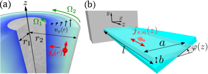
Taylor-Couette Flow.—As an explicit example, let us consider a two-dimensional steady flow with concentric circular streamlines. In this case, the flow velocity is parallel to the $\varphi$-direction, $\bm{v}=(0,v_{\varphi},0)$, satisfying the following Navier-Stokes equation: $\partial_{r}^{2}v_{\varphi}+(\partial_{r}v_{\varphi})/r-v_{\varphi}/r^{2}=0$. The general solution is $v_{\varphi}=c_{1}/r+c_{2}r$ with integration constants $c_{1}$ and $c_{2}$ determined by boundary conditions. The first term represents irrotational flow, while the second term represents rigid-rotation flow. We consider the two infinitely long coaxial cylinders of radii $r_{1}$ and $r_{2}$ ($r_{2}>r_{1}$), and the inner and outer cylinders are rotating at constant angular velocities $\Omega_{1}$ and $\Omega_{2}$, respectively. Under these boundary conditions, $v_{\varphi}(r_{1})=r_{1}\Omega_{1}$ and $v_{\varphi}(r_{2})=r_{2}\Omega_{2}$, the constants are obtained as $c_{1}=(\Omega_{1}-\Omega_{2})r_{1}^{2}r_{2}^{2}/(r_{2}^{2}-r_{1}^{2})$ and $c_{2}=(\Omega_{2}r_{2}^{2}-\Omega_{1}r_{1}^{2})/(r_{2}^{2}-r_{1}^{2})$. This concentric steady flow, known as the Taylor-Couette flow [43], induces the steady differential rotation with angular velocity $\Omega(r)=c_{1}/r^{2}+c_{2}$, leading to the generation of spin current (see Fig. 1(a)):

where $\bm{e}_{r}$ being the unit vector in the $r$-direction. Notably, since the vorticity in this system is constant, $\bm{\nabla}\times\bm{v}=2c_{2}\bm{e}_{z}$, the conventional spin currents owing to the spin-vorticity coupling, which require the vorticity gradient [44, 35] or time-dependent vorticity [45], do not appear. On the other hand, our theory predicts the generation of spin current even in vorticity-free cases $c_{2}=0$.

To estimate the magnitude of the spin current, we assume that the radii of the two cylinders are much larger than the gap between them $d=r_{2}-r_{1}$, i.e., $r_{1},r_{2}\gg d$, and only the outer cylinder is rotating, $\Omega_{1}=0$ and $\Omega_{2}\neq 0$, for simplicity. Under this assumption, the spin current is approximated as $j_{s}=\hbar\sigma_{c}\Omega_{2}/2e^{2}d$. We consider (Ga,In)Sn as the fluid with the electric conductivity $\sigma_{c}=3.26\times 10^{6}(\Omega\cdot\text{m})^{-1}$ [38]. Set $d\sim 1\mu$m and $\Omega_{2}\sim 10^{2}$kHz, the magnitude of the spin current in charge current units is estimated as $ej_{s}\sim 1.07\times 10^{2}\text{A$\cdot$m${}^{-2}$}$.

Torsional Oscillation of Cantilever.—As another example, we focus on the torsional oscillation of a cantilever, wherein one of the ends is securely fixed while external forces are exerted on the opposite end. These forces induce only a twisting motion in the cantilever, not bending or other deformations. In this case, the angular velocity of the system varies along the rotation axis rather than the radial direction. The distortion angle $\varphi(z,t)$ of the cantilever dictates the subsequent equation of motion: $C\partial_{z}^{2}\varphi=\rho_{m}I\partial_{t}^{2}\varphi$, where $C$ is the torsional rigidity, $\rho_{m}$ is the mass density, and $I$ is the moment of inertia of the cross-section about its center of mass. By solving the equation of motion under the boundary conditions $\varphi(0,t)=0$ and $\partial_{z}\varphi(l,t)=0$ and considering the initial conditions $\varphi(l,0)=\varphi_{0}$ and $\partial_{t}\varphi(z,0)=0$, we derive the solution as $\varphi_{n}(z,t)=\varphi_{0}\sin k_{n}z\cos\omega_{n}t$, where $k_{n}=(2n-1)\pi/2l$ and $\omega_{n}=vk_{n}$ with the integer $n\geq 1$ and the velocity $v=\sqrt{C/\rho_{m}I}$. The spin current, driven by the $n$-th torsional oscillation of cantilever, flows along the $z$-direction as given by (see Fig. 1(b))

The mechanism under investigation in this study represents a universal phenomenon, irrespective of material choice, and fundamentally distinct from the previous theory [46] that focus solely on magnetic materials.

Finally, we estimate the magnitude of the spin current driven by the torsional oscillation. For a plate-shaped cantilever with width $a$, thickness $b$ and length $l$, the quantities $C$ and $I$ are calculated as $C\simeq\mu ab^{3}/3$ and $I\simeq a^{3}b/12$ ($a\gg b$) with Lamé constant $\mu$. The magnitude of the total spin current in charge current units is denoted by $J_{n}=eabj_{s,n}(0,0)$, while that attributed to the first torsional oscillation mode is given by $J_{1}=(\pi^{2}\hbar\sigma_{c}\varphi_{0}/4e)(b/l)^{2}\sqrt{\mu/\rho_{m}}$. We consider that the cantilever is composed of copper with weak spin-orbit interaction. By using the charge conductivity $\sigma_{c}=6.45\times 10^{7}\,\Omega^{-1}\text{m}^{-1}$, the Lamé constant $\mu=48.3\,\text{GHz}$ and the mass density $\rho_{m}=8.96\times 10^{3}\,\text{kg}/\text{m}^{3}$, the total spin current is estimated as $J_{1}\sim 0.15\,\mu$A for $\varphi_{0}\sim 0.01$ and $b/l=1/4$.

Conclusion and discussion.— We studied non-equilibrium spin dynamics in differentially rotating systems within a microscopic theory. We obtained a Hamiltonian with emergent gauge fields by using a mapping to the comoving frame of the differential rotation. We estimated the spin currents generated by differential rotation in a liquid metal and a non-magnetic metallic nanomechanical system for experimental reference. Our mechanism produces spin currents even in vorticity-free systems. Hence, this mechanism of spin current generation is novel and distinct from the known mechanisms based on the spin-vorticity coupling.

Distinctions between our mechanism and those proposed in other literature [45, 44, 35] can be summarized as follows. In terms of spin transport equations, the source terms that violate the conservation of the spin density differ in the mechanisms. The spin current is proportional to the spatial gradient of these source terms. For our case, the spin transport equation is given in (15) and the source term is proportional to $\Omega$, the angular velocity of the orbital rotation around a fixed axis. On the other hand, the source term given in [45] and those in [44, 35] are proportional to $\partial_{t}\tilde{\omega}$ and $\tilde{\omega}$, respectively, where $\tilde{\omega}$ is the vorticity. These distinctions can be detected experimentally. In an irrotational flow, the vorticity is zero, preventing the spin current generation due to the spin-vorticity coupling. Creating an irrotational flow akin to a differentially rotating system allows us to detect spin currents specific to our mechanism. One may achieve such flow in the Taylor-Couette flow by taking appropriate boundary conditions that realize $c_{2}=0$ with $c_{1}\neq 0$. Furthermore, we can distinguish the mechanisms even in the case of $c_{2}\neq 0$. Since the vorticity in this system is uniform and time-independent, neither the source term in [45] nor that in [44, 35] can contribute to the spin current. As a result, the Taylor-Couette flow can generate the spin current in our mechanism but not in the other ones. Exploring these experiments would be highly valuable.

We have comments on possible pictures that come from (13). If we interpret $A_{s,0}=\partial_{t}\Phi$ as a “chemical potential” for the spin density, (13) suggests that the diffusive spin current is produced as a result of the position-dependent “chemical potential” for the spin density. Also, rewriting (13) as $\bm{j}_{s}(\bm{x},t)/n_{e}=[-(\hbar/2)\bm{\nabla}\partial_{t}\Phi]\tau/m$, we may interpret that a “thermodynamic force” $-(\hbar/2)\bm{\nabla}\partial_{t}\Phi$ is acting on the electrons depending on their spin, since $\tau/m$ is the mobility of the electron and $\bm{j}_{s}(\bm{x},t)/n_{e}$ can be understood as the mean velocity of the electrons. These interpretations should be further refined by future studies.

Acknowledgements.—We would like to thank D. Oue and Y. Nozaki for the valuable and informative discussion. This work was partially supported by JST CREST Grant No. JPMJCR19J4, Japan. We acknowledge JSPS KAKENHI for Grants (Nos. JP21H01800, JP21H04565, JP23H01839, JP21H05186, JP19K03659, JP19H05821, JP18K03623 and JP21H05189). The work was supported in part by the Chuo University Personal Research Grant. The authors thank RIKEN iTHEMS NEW working group for providing the genesis of this collaboration.

References

- Maekawa et al. [2017] S. Maekawa, S. O. Valenzuela, E. Saitoh, and T. Kimura, Spin current, Vol. 22 (Oxford University Press, 2017).
- Uchida et al. [2011] K.-i. Uchida, T. An, Y. Kajiwara, M. Toda, and E. Saitoh, Surface-acoustic-wave-driven spin pumping in Y3Fe5O12/Pt hybrid structure, Appl. Phys. Lett. 99, 212501 (2011).
- Weiler et al. [2012] M. Weiler, H. Huebl, F. S. Goerg, F. D. Czeschka, R. Gross, and S. T. B. Goennenwein, Spin Pumping with Coherent Elastic Waves, Phys. Rev. Lett. 108, 176601 (2012).
- Deymier et al. [2014] P. A. Deymier, J. O. Vasseur, K. Runge, A. Manchon, and O. Bou-Matar, Phonon-magnon resonant processes with relevance to acoustic spin pumping, Phys. Rev. B 90, 224421 (2014).
- Puebla et al. [2020] J. Puebla, M. Xu, B. Rana, K. Yamamoto, S. Maekawa, and Y. Otani, Acoustic ferromagnetic resonance and spin pumping induced by surface acoustic waves, J. Phys. D: Appl. Phys. 53, 264002 (2020).
- Al Misba et al. [2020] W. Al Misba, M. M. Rajib, D. Bhattacharya, and J. Atulasimha, Acoustic-Wave-Induced Ferromagnetic-Resonance-Assisted Spin-Torque Switching of Perpendicular Magnetic Tunnel Junctions with Anisotropy Variation, Phys. Rev. Applied 14, 014088 (2020).
- Camara et al. [2019] I. Camara, J.-Y. Duquesne, A. Lemaître, C. Gourdon, and L. Thevenard, Field-Free Magnetization Switching by an Acoustic Wave, Phys. Rev. Applied 11, 014045 (2019).
- Tateno et al. [2020] S. Tateno, G. Okano, M. Matsuo, and Y. Nozaki, Phys. Rev. B 102, 104406 (2020).
- Kawada et al. [2021] T. Kawada, M. Kawaguchi, T. Funato, H. Kohno, and M. Hayashi, Acoustic spin Hall effect in strong spin-orbit metals, Sci. Adv. 7, eabd9697 (2021).
- Sasaki et al. [2017] R. Sasaki, Y. Nii, Y. Iguchi, and Y. Onose, Nonreciprocal propagation of surface acoustic wave in Ni / LiNbO 3, Phys. Rev. B 95, 020407 (2017).
- Tateno and Nozaki [2020] S. Tateno and Y. Nozaki, Highly nonreciprocal spin waves excited by magnetoelastic coupling in a Ni/Si bilayer, Phys. Rev. Applied 13, 034074 (2020).
- Xu et al. [2020] M. Xu, K. Yamamoto, J. Puebla, K. Baumgaertl, B. Rana, K. Miura, H. Takahashi, D. Grundler, S. Maekawa, and Y. Otani, Nonreciprocal surface acoustic wave propagation via magneto-rotation coupling, Science Advances 6, eabb1724 (2020).
- Küß et al. [2021] M. Küß, M. Heigl, L. Flacke, A. Hörner, M. Weiler, A. Wixforth, and M. Albrecht, Nonreciprocal magnetoacoustic waves in dipolar-coupled ferromagnetic bilayers, Phys. Rev. Appl. 15, 034060 (2021).
- Matsumoto et al. [2022] H. Matsumoto, T. Kawada, M. Ishibashi, M. Kawaguchi, and M. Hayashi, Large surface acoustic wave nonreciprocity in synthetic antiferromagnets, Appl. Phys. Express 15, 063003 (2022).
- Lyons et al. [2023] T. P. Lyons, J. Puebla, K. Yamamoto, R. S. Deacon, Y. Hwang, K. Ishibashi, S. Maekawa, and Y. Otani, Acoustically Driven Magnon-Phonon Coupling in a Layered Antiferromagnet, Phys. Rev. Lett. 131, 196701 (2023).
- Chowdhury et al. [2017] P. Chowdhury, A. Jander, and P. Dhagat, Nondegenerate Parametric Pumping of Spin Waves by Acoustic Waves, IEEE Magnetics Letters 8, 1 (2017).
- Alekseev et al. [2020] S. G. Alekseev, S. E. Dizhur, N. I. Polzikova, V. A. Luzanov, A. O. Raevskiy, A. P. Orlov, V. A. Kotov, and S. A. Nikitov, Magnons parametric pumping in bulk acoustic waves resonator, Applied Physics Letters 117, 072408 (2020).
- Liao et al. [2023] L. Liao, J. Puebla, K. Yamamoto, J. Kim, S. Maekawa, Y. Hwang, Y. Ba, and Y. Otani, Valley-Selective Phonon-Magnon Scattering in Magnetoelastic Superlattices, Phys. Rev. Lett. 131, 176701 (2023).
- Barnett [1915] S. J. Barnett, Phys. Rev. 6, 239 (1915).
- A. Einstein and de Haas [1915] A. Einstein and W. J. de Haas, Proc. KNAW 18, 696 (1915).
- Scott [1962] G. Scott, Review of gyromagnetic ratio experiments, Reviews of Modern Physics 34, 102 (1962).
- [22] T. M. Wallis, J. Moreland, and P. Kabos, Einstein–de Haas effect in a NiFe film deposited on a microcantilever, Applied Physics Letters 89, 122502.
- [23] G. Zolfagharkhani, A. Gaidarzhy, P. Degiovanni, S. Kettemann, P. Fulde, and P. Mohanty, Nanomechanical detection of itinerant electron spin flip, Nature Nanotechnology 3, 720.
- [24] K. Harii, Y.-J. Seo, Y. Tsutsumi, H. Chudo, K. Oyanagi, M. Matsuo, Y. Shiomi, T. Ono, S. Maekawa, and E. Saitoh, Spin Seebeck mechanical force, Nature Communications 10, 2616.
- [25] K. Mori, M. G. Dunsmore, J. E. Losby, D. M. Jenson, M. Belov, and M. R. Freeman, Einstein–de Haas effect at radio frequencies in and near magnetic equilibrium, Physical Review B 102, 054415.
- Chudo et al. [2014] H. Chudo, M. Ono, K. Harii, M. Matsuo, J. Ieda, R. Haruki, S. Okayasu, S. Maekawa, H. Yasuoka, and E. Saitoh, Appl. Phys. Express 7, 063004 (2014).
- Chudo et al. [2015] H. Chudo, K. Harii, M. Matsuo, J. Ieda, M. Ono, S. Maekawa, and E. Saitoh, J. Phys. Soc. Jpn. 84, 043601 (2015).
- [28] M. Arabgol and T. Sleator, Observation of the Nuclear Barnett Effect, Physical Review Letters 122, 177202.
- Chudo et al. [2021] H. Chudo, M. Matsuo, S. Maekawa, and E. Saitoh, Phys. Rev. B 103, 174308 (2021).
- Wood et al. [2017] A. Wood, E. Lilette, Y. Fein, V. Perunicic, L. Hollenberg, R. Scholten, and A. Martin, Magnetic pseudo-fields in a rotating electron–nuclear spin system, Nature Physics 13, 1070 (2017).
- Hirohata et al. [2018] A. Hirohata, Y. Baba, B. A. Murphy, B. Ng, Y. Yao, K. Nagao, and J.-y. Kim, Magneto-optical detection of spin accumulation under the influence of mechanical rotation, Scientific reports 8, 1974 (2018).
- [32] C. Dornes, Y. Acremann, M. Savoini, M. Kubli, M. J. Neugebauer, E. Abreu, L. Huber, G. Lantz, C. A. F. Vaz, H. Lemke, E. M. Bothschafter, M. Porer, V. Esposito, L. Rettig, M. Buzzi, A. Alberca, Y. W. Windsor, P. Beaud, U. Staub, D. Zhu, S. Song, J. M. Glownia, and S. L. Johnson, The ultrafast Einstein–de Haas effect, Nature 565, 209.
- [33] M. Ganzhorn, S. Klyatskaya, M. Ruben, and W. Wernsdorfer, Quantum Einstein-de Haas effect, Nature Communications 7, 11443.
- Adamczyk et al. [2017] L. Adamczyk, J. Adkins, G. Agakishiev, M. Aggarwal, Z. Ahammed, N. Ajitanand, I. Alekseev, D. Anderson, R. Aoyama, A. Aparin, et al., Global hyperon polarization in nuclear collisions, Nature 548 (2017).
- Takahashi et al. [2016] R. Takahashi, M. Matsuo, M. Ono, K. Harii, H. Chudo, S. Okayasu, J. Ieda, S. Takahashi, S. Maekawa, and E. Saitoh, Nature Phys 12, 52 (2016).
- Kobayashi et al. [2017] D. Kobayashi, T. Yoshikawa, M. Matsuo, R. Iguchi, S. Maekawa, E. Saitoh, and Y. Nozaki, Phys. Rev. Lett. 119, 077202 (2017).
- Takahashi et al. [2020] R. Takahashi, H. Chudo, M. Matsuo, K. Harii, Y. Ohnuma, S. Maekawa, and E. Saitoh, Nat Commun 11, 3009 (2020).
- Tabaei Kazerooni et al. [2020] H. Tabaei Kazerooni, A. Thieme, J. Schumacher, and C. Cierpka, Phys. Rev. Applied 14, 014002 (2020).
- Tabaei Kazerooni et al. [2021] H. Tabaei Kazerooni, G. Zinchenko, J. Schumacher, and C. Cierpka, Phys. Rev. Fluids 6, 043703 (2021).
- Tateno et al. [2021] S. Tateno, Y. Kurimune, M. Matsuo, K. Yamanoi, and Y. Nozaki, Phys. Rev. B 104, L020404 (2021).
- Hehl and Ni [1990] F. W. Hehl and W.-T. Ni, Inertial effects of a dirac particle, Physical Review D 42, 2045 (1990).
- Funato and Kohno [2018] T. Funato and H. Kohno, J. Phys. Soc. Jpn. 87, 073706 (2018).
- Taylor [1923] G. I. Taylor, Philos. Trans. R. Soc. London, Ser. A 223, 289 (1923).
- Matsuo et al. [2017] M. Matsuo, Y. Ohnuma, and S. Maekawa, Phys. Rev. B 96, 020401 (2017).
- Matsuo et al. [2013] M. Matsuo, J. Ieda, K. Harii, E. Saitoh, and S. Maekawa, Phys. Rev. B 87, 180402 (2013).
- Fujimoto and Matsuo [2020] J. Fujimoto and M. Matsuo, Magnon current generation by dynamical distortion, Phys. Rev. B 102, 020406 (2020).
I Transformation to differentially rotating frame
By using the total angular momentum operator acting on coordinates and spin space,