Spike-NeRF: Neural Radiance Field Based On Spike Camera
Abstract
As a neuromorphic sensor with high temporal resolution, spike cameras offer notable advantages over traditional cameras in high-speed vision applications such as high-speed optical estimation, depth estimation, and object tracking. Inspired by the success of the spike camera, we proposed Spike-NeRF, the first Neural Radiance Field derived from spike data, to achieve 3D reconstruction and novel viewpoint synthesis of high-speed scenes. Instead of the multi-view images at the same time of NeRF, the inputs of Spike-NeRF are continuous spike streams captured by a moving spike camera in a very short time. To reconstruct a correct and stable 3D scene from high-frequency but unstable spike data, we devised spike masks along with a distinctive loss function. We evaluate our method qualitatively and numerically on several challenging synthetic scenes generated by blender with the spike camera simulator. Our results demonstrate that Spike-NeRF produces more visually appealing results than the existing methods and the baseline we proposed in high-speed scenes. Our code and data will be released soon.
Index Terms:
Neuromorphic Vision, Spike Camera, Neural Radiance Field.I Introduction
Novel-view synthesis (NVS) is a long-standing problem aiming to render photo-realistic images from novel views of a scene from a sparse set of input images. This topic has recently seen impressive progress due to the use of neural networks to learn representations that are well suited for view synthesis tasks, known as Neural Radiance Field (NeRF)[1, 2, 3, 4, 5, 6, 7]. Despite its success, NeRF performs awfully in high-speed scenes since the motion blur caused by high-speed scenes violates the assumption by NeRF that the input images are sharp. Deblur methods such as Deblur-NeRF [8] and BAD-NeRF[9] can only handle mild motion blur. The introduction of high-speed neuromorphic cameras, such as event cameras [10] and spike cameras, are expected to fundamentally solve this problem.
Spike camera [11, 12] is a neuromorphic sensor, where each pixel captures photons independently, keeps recording the luminance intensity asynchronously, and outputs binary spike streams to record the dynamic scenes at extremely high temporal resolution (40000Hz). Recently, many existing approaches use spike data to reconstruct image [13, 14, 15] for high-speed scenes, or directly perform downstream tasks such as optical flow estimation [16] and depth estimation [17].
Motivated by the notable success achieved by spike cameras and NeRF’s
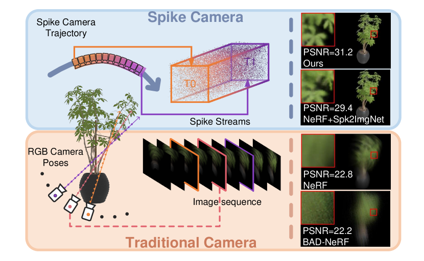
limitation, we proposed Spike-NeRF, the first Neural Radiance Field built by spike data. Different from NeRF, we use a set of continuously spike streams as inputs instead of images from different perspectives at the same time (see Figure 1). To reconstruct a volumetric 3D representation of a scene from spike streams and generate a new spike stream for novel views based on this scene, we first proposed a spiking volume renderer based on the coding method of spike cameras. It generates spike streams asynchronously with radiance obtained by ray casting. Additionally, we both use spike loss to reduce local blur and spike masks to limit NeRF learning information in a specific area, thereby mitigating artifacts resulting from reconstruction errors and noise.
Our experimental results show that Spike-NeRF is suitable for high-speed scenes that would not be conceivable with traditional cameras. Moreover, our method is largely superior to directly using reconstructed images of spike streams for supervision which is considered as the baseline. Our main contributions can be summarized as follows:
-
Spike-NeRF, the first approach for inferring NeRF from a spike stream that enables a novel view synthesis in both gray and RGB space for high-speed scene.
-
A bespoke rendering strategy for spike streams leading to data-efficient training and spike stream generating.
-
A dataset containing RGB spike data and high-frequency (40,000fps) camera poses
II Related Work
II-A NeRF on traditional cameras
Neural Radiance Field (NeRF) [1] has arisen as a significant development in the field of Computer Vision and Computer Graphics, used for synthesizing novel views of a scene from a sparse set of images by combining machine learning with geometric reasoning. Various research and approaches based on NeRF have been proposed recently. For example, [18, 19, 20, 21] extend NeRF to dynamic and non-grid scenes, [2, 3] significantly improve the rendering quality of NeRF and [9, 8, 22, 23] robustly severe blurred images that could affect the rendering quality of NeRF.
II-B NeRF on Neuromorphic Cameras
Neuromorphic sensors have shown their advantages in most computer version problems including novel views synthesizing. EventNeRF [24] and Ev-nerf [25] synthesize the novel view in scenarios such as high-speed movements that would not be conceivable with a traditional camera by event supervision. Nonetheless, these works assume that event streams are temporally dense and low-noise which is inaccessible in practice. Robust e-NeRF [26] incorporates a more realistic event generation model to directly and robustly reconstruct NeRFs under various real-world conditions. DE-NeRF [27] and E2NeRF [28] extend event nerf to dynamic scenes and severely blurred images as NeRF researchers did.
II-C Spike Camera Application
As a neuromorphic sensor with high temporal resolution, spike cameras [12] offer significant advantages on many high-speed version tasks. [29] and [13] propose spike stream reconstruction methods for high-speed scenes. Subsequently, deep learning-based reconstruction frameworks [14, 15] are introduced to reconstruct spike streams robustly. Spike cameras also show its superiors on downstream tasks such as optical flow estimation [16, 30], monocular and stereo depth estimation [17, 31], Super-resolution [32] and high-speed real-time object tracking [33].
III Preliminary
III-A Spike Camera And Its Coding Method
Unlike traditional cameras that record the luminance intensity of each pixel during the exposure time at a fixed frame rate, tensors on spike cameras of each pixel capture photons independently and keep recording the luminance intensity asynchronously without a dead zone.
Each pixel on the spike camera converts the light signal into a current signal. When the accumulated intensity reaches the dispatch threshold, a spike is fired and the accumulated intensity is reset. For pixel ,this process can be expressed as
| (1) |
| (2) |
where:
| (3) |
Here is the accumulated intensity at time , is the spike output at time and is the input current at time (proportional to light intensity). We will directly use to represent the luminance intensity to simplify our presentation. Further, due to the limitations of circuits, each spike is read out at discrete time ( is a micro-second level). Thus, the output of the spike camera is a spatial-temporal binary stream with size. Here, and are the height and width of the sensor, respectively, and is the temporal window size of the spike stream.
III-B Neural Radiance Field (NeRF) Theory
Neural Radiance Field (NeRF) uses a 5D vector-valued function to represent a continuous scene. The input to this function consists of a 3D location x = (x, y, z) and 2D viewing direction d =(,), while output is an emitted color c = (r, g, b) and volume density . Both and c are represented implicitly as multi-layer perceptrons (MLPs), written as:
| (4) |
Given the volume density and color functions c, the rendering result of any given ray passes through the scene can be computed using principles from volume rendering.
| (5) |
where
| (6) |
The function T(t) denotes the accumulated transmittance along the ray from to t. For computing reasons, rays were divided into N equally spaced bins, and a sample was uniformly drawn from each bin. Then, equation 5 can be approximated as
| (7) |
where:
| (8) |
and:
| (9) |
After calculating the color for each pixel, a square error photometric loss is used to optimize the MLP parameters.
| (10) |
IV Method
IV-A Overview
Taking inspiration from NeRF, Spike-NeRF implicitly represents the static scenes as an MLP network with 5D inputs:
| (11) |
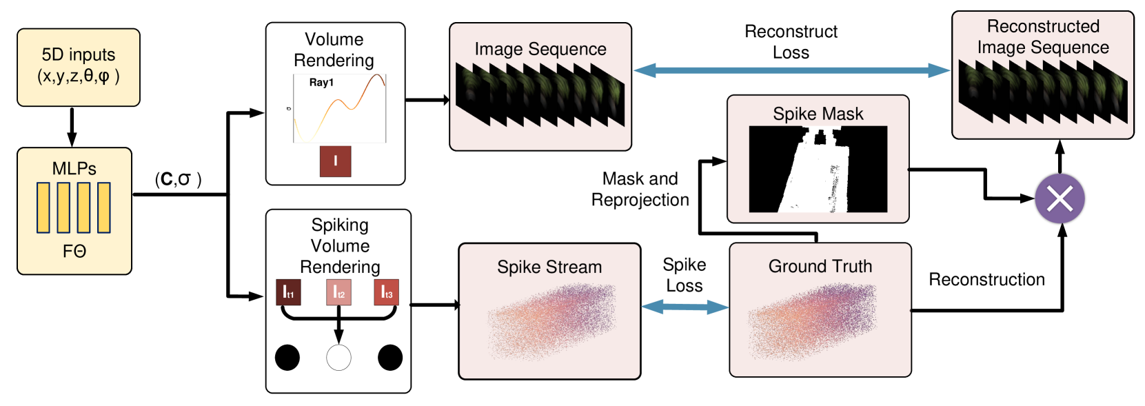
Here, each corresponds to a frame of spike in the continuous spike stream captured by a spike camera in a very short time. Considering the difficulty of directly using spike streams for supervision, we firstly reconstruct the spike stream into image sequence where is the reconstructed image at . We use the results with inputs= as our baseline. Since all methods reconstruct images from multi-frame spikes, using the reconstructed images as a supervision signal would lead to artifacts and blurring. We introduce spike masks to make NeRF focus on the triggered area. We also propose a spiking volume renderer based on the coding method of the spike camera to generate spike streams for novel views. We then use the g.t. spike streams constraint network directly.
The total loss used to train Spike-NeRF is given by:
| (12) |
is the loss between the image rendering result and masked images which are reconstructed from g.t. spike streams. is the loss between the spike rendering result generated by our spiking volume rendering method and g.t. spike streams.
IV-B Spiking Volume Renderer
If we introduce time into the volume rendering equation 5, the rendering results of any given ray at time is:
| (13) |
Where
| (14) |
Then, if we assume that for any , equation LABEL:ax can be written as:
| (15) |
Here, is the threshold of the spike camera and N is the number of ”1” for spike streams and x=(x,y) is the coordinates for each pixel. For computing reasons, rays were divided into equally spaced bins, were divided into equally spaced bins, and a sample was uniformly drawn from each bin. Then, equation 2 can be written as:
| (16) |
where:
| (17) |
where:
| (18) |
and:
| (19) |
However, is not equal to 0 in real situations. To address this, we introduce a random startup matrix and utilize the stable results after several frames. The above processes do not participate in backpropagation as they are not differentiable. After generating spike streams , we can compute:
| (20) |
IV-C Spike Masks
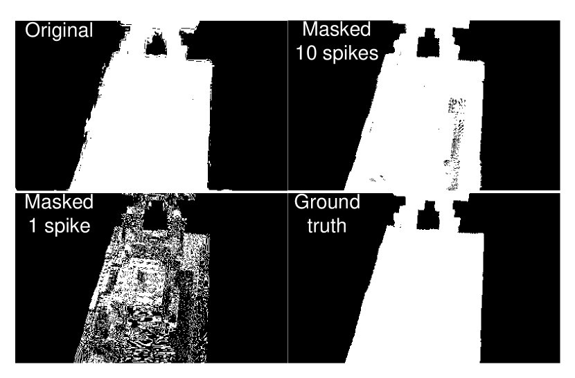
Due to the serious lack of information in a single spike, all reconstruction methods use multi-frame spikes as input. These methods can reconstruct images with detailed textures from spike streams, but can also introduce erroneous information due to the use of preceding and following frame spikes (see Figure 4 original), which results in foggy edges in the scene learned by NeRF. We introduce spike masks to solve this problem.
| Dataset | chair_rgb | drums_rgb | ficus_rgb | hotdog_rgb | lego_rgb | materials_rgb | average_rgb | |||||||
| Method Metrics | SSIM | PSNR | SSIM | PSNR | SSIM | PSNR | SSIM | PSNR | SSIM | PSNR | SSIM | PSNR | SSIM | PSNR |
| NeRF | 0.754 | 21.14 | 0.593 | 21.40 | 0.707 | 22.31 | 0.752 | 19.31 | 0.455 | 17.24 | 0.533 | 18.36 | 0.632 | 19.96 |
| BAD-Nerf[cvpr23] | 0.604 | 19.44 | 0.563 | 20.70 | 0.597 | 20.97 | 0.658 | 19.42 | 0.385 | 16.02 | 0.397 | 17.56 | 0.534 | 19.02 |
| NeRF+Spk2ImgNet[cvpr21] | 0.961 | 32.21 | 0.899 | 29.90 | 0.908 | 27.80 | 0.920 | 28.92 | 0.837 | 26.00 | 0.877 | 28.27 | 0.901 | 28.85 |
| Ours | 0.973 | 32.90 | 0.922 | 30.16 | 0.936 | 29.10 | 0.923 | 29.69 | 0.861 | 26.32 | 0.912 | 28.67 | 0.921 | 29.48 |
| Dataset | chair_gray | drums_gray | ficus_gray | hotdog_gray | lego_gray | materials_gray | average_gray | |||||||
| Methods Metrics | SSIM | PSNR | SSIM | PSNR | SSIM | PSNR | SSIM | PSNR | SSIM | PSNR | SSIM | PSNR | SSIM | PSNR |
| NeRF | 0.662 | 17.09 | 0.437 | 15.85 | 0.628 | 16.59 | 0.243 | 18.06 | 0.292 | 14.06 | 0.365 | 14.34 | 0.438 | 16.00 |
| BAD-Nerf[cvpr23] | 0.646 | 15.12 | 0.510 | 14.38 | 0.624 | 16.18 | 0.431 | 15.87 | 0.372 | 11.91 | 0.341 | 12.60 | 0.487 | 14.34 |
| NeRF+Spk2ImgNet[cvpr21] | 0.803 | 27.36 | 0.671 | 23.58 | 0.827 | 24.79 | 0.528 | 25.47 | 0.636 | 22.97 | 0.615 | 23.12 | 0.680 | 24.55 |
| Ours | 0.881 | 31.70 | 0.764 | 25.81 | 0.874 | 26.18 | 0.581 | 26.79 | 0.710 | 25.07 | 0.769 | 25.43 | 0.763 | 26.83 |
Because of the spatial sparsity of the spike streams, using a single spike mask will lead to a large number of cavities. To address this, we use a relatively small number of multi-frame spikes to fill the cavities. Considering spike at time and reconstruction result , we first choose as original mask sequence. Finally, we have:
| (21) |
where means or. After masking image sequence , we can compute:
| (22) |
V Experiment
We adopt Novel View Synthesis (NVS) as the standard task to verify our method. We first compare our method with NeRF approaches on traditional cameras and the proposed baseline. We then conduct comprehensive quantitative ablation studies to illustrate the usage of the designed modules.
V-A Implementation Details
Our code is based on NeRF [1] and we train the models for iterations on one NVIDIA A100 GPU with the same optimizer and hyper-parameters as NeRF. Since the spiking volume renderer requires continuous multi-spikes, we select the camera pose and sampling points for spiking volume rendering determinedly rather than randomly as NeRF did. We examined our method on synthetic sequences from NeRF [1]. We examined six scenes(lego, ficus, chair, materials, hotdog and drums) which cover different conditions. We rendered all of them with a 0.025-second-long 360-degree rotation of the camera around the object resulting in 1000 views to simulate the 40000 fps spike camera and other blurred images in 1000 views to simulate the 400 fps high-speed traditional camera by Blender. Like NeRF, we directly use the corresponding camera intrinsics and extrinnsics generated by the blender.
V-B Comparisons against other Methods
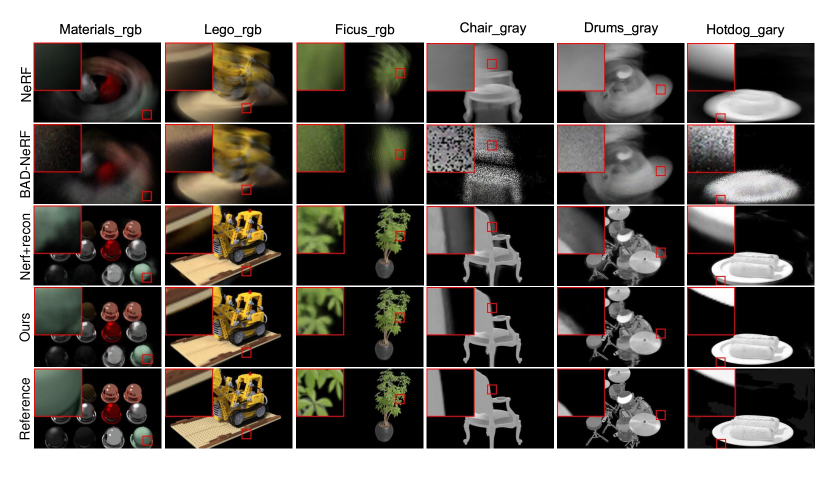
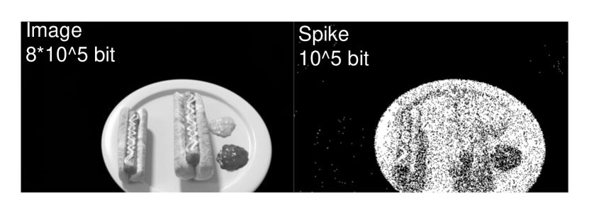
We compare the spike NeRF results with three baselines: Spk2ImgNet+NeRF[14], the 400 fps traditional camera results on NeRF and BAD-NeRF[9](see Figure 3).To better demonstrate the adaptability of our method to spike cameras, we show both gray and RGB results. From Figure 3 we know that our method has absolute advantages over NeRF and BAD-NeRF in high-speed scenes. Compared with directly using spike reconstruction results for training, our method also has obvious supervisors. Corresponding numerical results are reported in Table I from what we can conclude our method improves more in gray space. We also compared the data sizes of two modalities: spikes and images. From Figure 5 we can conclude that spikes have less information resulting in noise and loss of detail. However, our method leverages temporal consistency (see section IV) to derive stable 3D representations from information-lacking and unstable spike streams.
| MethodsMetrics | SSIM | PSNR | LPIPS |
| W/O spike masks | 0.899 | 28.97 | 0.064 |
| W/O spike loss | 0.918 | 29.18 | 0.067 |
| Full | 0.921 | 29.48 | 0.061 |
V-C Ablation
Compared with baselines, our Spike-NeRF introduces two main components: spike masks and the spike volume renderer with spike loss. Next, we discuss their impact on the results.
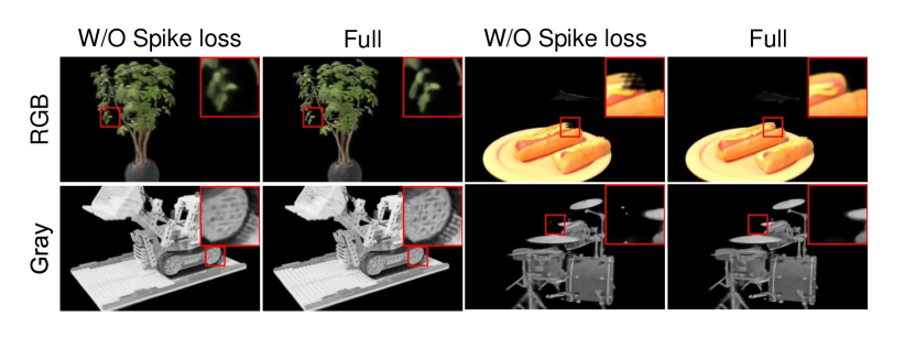
Spike Loss: In section IV, we proposed spike loss to solve the cavities caused by the partial information loss due to spike masks and the blur caused by incorrect reconstruction. Figure 6 shows the results before and after disabling spike loss. From Figure 6 we know that after disabling spike loss, some scenes have obvious degradation in details and a large number of wrong holes. TabII shows the improvement of the spike loss.
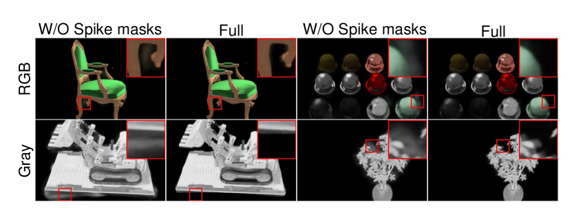
Spike masks: Incorrect reconstruction will also lead to a large number of artifacts in NeRF results. We use spike masks to eliminate artifacts to the maximum extent (see IV). Figure 7 shows the results before and after disabling spike masks. From Figure 7 we know that after disabling spike masks, all scenes have obvious artifacts. TabII shows the improvement of the spike masks.
VI Conclusion
We introduced the first approach to reconstruct a 3D scene from spike streams which enables photorealistic novel view synthesis in both gray and RGB space. Thanks to the high temporal resolution and unique coding method of the spike camera, Spike-Nerf shows credible advantages in high-speed scenes. Further, we proposed the spiking volume renderer and spike mask so that Spike NeRF outperforms baselines in terms of scene stability and texture details. Our method can also directly generate spike streams. To the best of our knowledge, our paper is also the first time that spike cameras have been used in the field of 3D representation.
Limitation: Due to the difficulty of collecting real spike data with camera poses, Spike-NeRF is only tested on synthetic datasets. In addition, Spike-NeRF assumes that the only moving object in the scene is the spike camera. We believe that NeRF based on spike cameras has greater potential in handling high-speed rigid and non-rigid motions for other objects. Future works can investigate it.
References
- [1] B. Mildenhall, P. P. Srinivasan, M. Tancik, J. T. Barron, R. Ramamoorthi, and R. Ng, “Nerf: Representing scenes as neural radiance fields for view synthesis,” Communications of the ACM, vol. 65, no. 1, pp. 99–106, 2021.
- [2] J. T. Barron, B. Mildenhall, M. Tancik, P. Hedman, R. Martin-Brualla, and P. P. Srinivasan, “Mip-nerf: A multiscale representation for anti-aliasing neural radiance fields,” in Proceedings of the IEEE/CVF International Conference on Computer Vision, 2021, pp. 5855–5864.
- [3] J. T. Barron, B. Mildenhall, D. Verbin, P. P. Srinivasan, and P. Hedman, “Mip-nerf 360: Unbounded anti-aliased neural radiance fields,” in Proceedings of the IEEE/CVF Conference on Computer Vision and Pattern Recognition, 2022, pp. 5470–5479.
- [4] R. Martin-Brualla, N. Radwan, M. S. Sajjadi, J. T. Barron, A. Dosovitskiy, and D. Duckworth, “Nerf in the wild: Neural radiance fields for unconstrained photo collections,” in Proceedings of the IEEE/CVF Conference on Computer Vision and Pattern Recognition, 2021, pp. 7210–7219.
- [5] A. Chen, Z. Xu, A. Geiger, J. Yu, and H. Su, “Tensorf: Tensorial radiance fields,” in European Conference on Computer Vision. Springer, 2022, pp. 333–350.
- [6] Z. Wang, S. Wu, W. Xie, M. Chen, and V. A. Prisacariu, “Nerf–: Neural radiance fields without known camera parameters,” arXiv preprint arXiv:2102.07064, 2021.
- [7] K. Zhang, G. Riegler, N. Snavely, and V. Koltun, “Nerf++: Analyzing and improving neural radiance fields,” arXiv preprint arXiv:2010.07492, 2020.
- [8] L. Ma, X. Li, J. Liao, Q. Zhang, X. Wang, J. Wang, and P. V. Sander, “Deblur-nerf: Neural radiance fields from blurry images,” in Proceedings of the IEEE/CVF Conference on Computer Vision and Pattern Recognition, 2022, pp. 12 861–12 870.
- [9] P. Wang, L. Zhao, R. Ma, and P. Liu, “Bad-nerf: Bundle adjusted deblur neural radiance fields,” in Proceedings of the IEEE/CVF Conference on Computer Vision and Pattern Recognition, 2023, pp. 4170–4179.
- [10] J.-W. Liu, Y.-P. Cao, W. Mao, W. Zhang, D. J. Zhang, J. Keppo, Y. Shan, X. Qie, and M. Z. Shou, “Devrf: Fast deformable voxel radiance fields for dynamic scenes,” Advances in Neural Information Processing Systems, vol. 35, pp. 36 762–36 775, 2022.
- [11] P. Joshi and S. Prakash, “Retina inspired no-reference image quality assessment for blur and noise,” Multimedia Tools and Applications, vol. 76, pp. 18 871–18 890, 2017.
- [12] S. Dong, T. Huang, and Y. Tian, “Spike camera and its coding methods,” arXiv preprint arXiv:2104.04669, 2021.
- [13] L. Zhu, J. Li, X. Wang, T. Huang, and Y. Tian, “Neuspike-net: High speed video reconstruction via bio-inspired neuromorphic cameras,” in Proceedings of the IEEE/CVF International Conference on Computer Vision, 2021, pp. 2400–2409.
- [14] J. Zhao, R. Xiong, H. Liu, J. Zhang, and T. Huang, “Spk2imgnet: Learning to reconstruct dynamic scene from continuous spike stream,” in Proceedings of the IEEE/CVF Conference on Computer Vision and Pattern Recognition, 2021, pp. 11 996–12 005.
- [15] J. Zhang, S. Jia, Z. Yu, and T. Huang, “Learning temporal-ordered representation for spike streams based on discrete wavelet transforms,” in Proceedings of the AAAI Conference on Artificial Intelligence, vol. 37, no. 1, 2023, pp. 137–147.
- [16] L. Hu, R. Zhao, Z. Ding, L. Ma, B. Shi, R. Xiong, and T. Huang, “Optical flow estimation for spiking camera,” in Proceedings of the IEEE/CVF Conference on Computer Vision and Pattern Recognition, 2022, pp. 17 844–17 853.
- [17] Y. Wang, J. Li, L. Zhu, X. Xiang, T. Huang, and Y. Tian, “Learning stereo depth estimation with bio-inspired spike cameras,” in 2022 IEEE International Conference on Multimedia and Expo (ICME). IEEE, 2022, pp. 1–6.
- [18] K. Park, U. Sinha, J. T. Barron, S. Bouaziz, D. B. Goldman, S. M. Seitz, and R. Martin-Brualla, “Nerfies: Deformable neural radiance fields,” in Proceedings of the IEEE/CVF International Conference on Computer Vision, 2021, pp. 5865–5874.
- [19] A. Pumarola, E. Corona, G. Pons-Moll, and F. Moreno-Noguer, “D-nerf: Neural radiance fields for dynamic scenes,” in Proceedings of the IEEE/CVF Conference on Computer Vision and Pattern Recognition, 2021, pp. 10 318–10 327.
- [20] Z. Li, S. Niklaus, N. Snavely, and O. Wang, “Neural scene flow fields for space-time view synthesis of dynamic scenes,” in Proceedings of the IEEE/CVF Conference on Computer Vision and Pattern Recognition, 2021, pp. 6498–6508.
- [21] Z. Yan, C. Li, and G. H. Lee, “Nerf-ds: Neural radiance fields for dynamic specular objects,” in Proceedings of the IEEE/CVF Conference on Computer Vision and Pattern Recognition, 2023, pp. 8285–8295.
- [22] D. Lee, M. Lee, C. Shin, and S. Lee, “Dp-nerf: Deblurred neural radiance field with physical scene priors,” in Proceedings of the IEEE/CVF Conference on Computer Vision and Pattern Recognition, 2023, pp. 12 386–12 396.
- [23] D. Lee, J. Oh, J. Rim, S. Cho, and K. M. Lee, “Exblurf: Efficient radiance fields for extreme motion blurred images,” in Proceedings of the IEEE/CVF International Conference on Computer Vision, 2023, pp. 17 639–17 648.
- [24] V. Rudnev, M. Elgharib, C. Theobalt, and V. Golyanik, “Eventnerf: Neural radiance fields from a single colour event camera,” in Proceedings of the IEEE/CVF Conference on Computer Vision and Pattern Recognition, 2023, pp. 4992–5002.
- [25] I. Hwang, J. Kim, and Y. M. Kim, “Ev-nerf: Event based neural radiance field,” in Proceedings of the IEEE/CVF Winter Conference on Applications of Computer Vision, 2023, pp. 837–847.
- [26] W. F. Low and G. H. Lee, “Robust e-nerf: Nerf from sparse & noisy events under non-uniform motion,” in Proceedings of the IEEE/CVF International Conference on Computer Vision, 2023, pp. 18 335–18 346.
- [27] Q. Ma, D. P. Paudel, A. Chhatkuli, and L. Van Gool, “Deformable neural radiance fields using rgb and event cameras,” in Proceedings of the IEEE/CVF International Conference on Computer Vision, 2023, pp. 3590–3600.
- [28] Y. Qi, L. Zhu, Y. Zhang, and J. Li, “E2nerf: Event enhanced neural radiance fields from blurry images,” in Proceedings of the IEEE/CVF International Conference on Computer Vision, 2023, pp. 13 254–13 264.
- [29] Y. Zheng, L. Zheng, Z. Yu, B. Shi, Y. Tian, and T. Huang, “High-speed image reconstruction through short-term plasticity for spiking cameras,” in Proceedings of the IEEE/CVF Conference on Computer Vision and Pattern Recognition, 2021, pp. 6358–6367.
- [30] S. Chen, Z. Yu, and T. Huang, “Self-supervised joint dynamic scene reconstruction and optical flow estimation for spiking camera,” in Proceedings of the AAAI Conference on Artificial Intelligence, vol. 37, no. 1, 2023, pp. 350–358.
- [31] J. Zhang, L. Tang, Z. Yu, J. Lu, and T. Huang, “Spike transformer: Monocular depth estimation for spiking camera,” in European Conference on Computer Vision. Springer, 2022, pp. 34–52.
- [32] J. Zhao, R. Xiong, J. Zhang, R. Zhao, H. Liu, and T. Huang, “Learning to super-resolve dynamic scenes for neuromorphic spike camera,” in Proceedings of the AAAI Conference on Artificial Intelligence, vol. 37, no. 3, 2023, pp. 3579–3587.
- [33] Y. Zheng, Z. Yu, S. Wang, and T. Huang, “Spike-based motion estimation for object tracking through bio-inspired unsupervised learning,” IEEE Transactions on Image Processing, vol. 32, pp. 335–349, 2022.