SPICE: Scaling-Aware Prediction Correction Methods with a Free Convergence Rate for Nonlinear Convex Optimization
Abstract
Recently, the prediction-correction method has been developed to solve nonlinear convex optimization problems. However, its convergence rate is often poor since large regularization parameters are set to ensure convergence conditions. In this paper, the scaling-aware prediction correction (Spice) method is proposed to achieve a free convergence rate. This method adopts a novel scaling technique that adjusts the weight of the objective and constraint functions. The theoretical analysis demonstrates that increasing the scaling factor for the objective function or decreasing the scaling factor for constraint functions significantly enhances the convergence rate of the prediction correction method. In addition, the Spice method is further extended to solve separable variable nonlinear convex optimization. By employing different scaling factors as functions of the iterations, the Spice method achieves convergence rates of , , and . Numerical experiments further validate the theoretical findings, demonstrating the effectiveness of the Spice method in practice.
keywords:
Primal-dual method, prediction correction method, scaling technique.1 Introduction
Nonlinear convex optimization is fundamental to many fields, including control theory, image denoising, and signal processing. This work addresses a general nonlinear convex problem with inequality constraints, formalized as:
| (1.1) |
where the set is a nonempty closed convex subset of . The objective and constraint function and are convex, with the constraint functions also being continuously differentiable. Notably, is not assumed to be differentiable. The Lagrangian function associated with P0, parameterized by the dual variable , is given by:
| (1.2) |
where , and the dual variable belongs to the set . In this way, the constrained problem is reformulated to a saddle point problem. The saddle point of (1.2) yields the optimal solution of P0. A common approach is to design an iterative scheme to update the primal and dual variables alternately. The Arrow-Hurwicz method, one of the earliest primal-dual methods, was proposed to solve concave-convex optimization problems [1], laying the foundation for subsequent developments. Sequentially, a primal-dual hybrid gradient (PDHG) method [2] introduced gradient steps, offering a more flexible framework. However, PDHG has been shown to diverge in certain linear programming problems [3], and its variants achieve convergence only under more restrictive assumptions [4]. To address this issue, the Chambolle-Pock method was developed as a modified version of PDHG. By introducing a relaxation parameter, it improved stability and enhanced the convergence rate for saddle point problems with linear operators [5, 6, 7]. Further extensions of PDHG have been applied to nonlinear operators [8, 9]. Unfortunately, these approaches offer only local convergence guarantees, leaving the convergence rate unaddressed. Another notable class of primal-dual methods is the customized proximal point algorithms (PPA) developed in [10, 11, 12, 13, 14]. These algorithms aim to customize a symmetric proximal matrix, rather than merely relaxing the primal variable, to address convex problems with linear constraints. Based on variational analysis theory, they provide a straightforward proof of convergence. Later, a novel prediction-correction (PC) method was proposed in [15, 16]. The key innovation of the PC method is proposed to correct the primal and dual variables generated by the Arrow-Hurwicz method without constructing a symmetric proximal matrix. This unified framework establishes convergence conditions for the corrective matrix, which are relatively easy to satisfy. In Table 1, a comparison of different primal-dual methods under setting assumptions and convergence rate.
Recent advances have extended prediction-correction (PC) methods to handle nonlinear optimization problems, particularly by leveraging carefully designed regularization parameters [17, 18]. These works prove that it can achieve ergodic convergence rates by ensuring that the sequence of regularization parameters is non-increasing. However, the design of such a sequence poses a significant challenge, as the regularization parameters strongly influence the performance of the proximal mapping problem. Larger regularization parameters, though useful in theory, often fail to capture the curvature of the proximal term effectively, leading to suboptimal convergence. While a smaller non-increasing sequence of regularization parameters can accelerate convergence toward the optimal solution, this approach introduces instability into the algorithm. The challenge, therefore, lies in balancing the size of these parameters to ensure both rapid convergence and algorithmic stability. The choice of these parameters is intricately tied to the derivative of the constraint functions; for any given derivative, a lower bound can be established on the product of the regularization parameters, which serves as a key condition for ensuring convergence. This lower bound prevents the parameters from being too small, while larger parameters are often inefficient at capturing the problem’s local shape, thereby slowing convergence rates. Building upon these theoretical foundations, some works have introduced customized proximal matrices to optimize regularization parameter selection. For instance, the authors of [19, 18] proposed generalized primal-dual methods that achieve a 25% reduction in the lower bound of the product of regularization parameters, representing a significant improvement in parameter tuning. Despite this progress, identifying smaller regularization parameters that still meet convergence conditions remains a major obstacle.
To solve this challenge, this paper introduces a novel scaling technique that adjusts the weights of the objective and constraint functions, enabling a reduction in the regularization parameters. This innovation leads to the development of the scaling-aware prediction correction (Spice) method, which achieves a free convergence rate for nonlinear convex problems, overcoming the limitations of existing approaches in terms of both stability and efficiency.
2 Preliminaries
This section introduces the foundational concepts, specifically the variational inequality, which is a key tool for the analysis later in the paper. Additionally, a scaling technique is proposed to adjust the variational inequality for further optimization.
2.1 Variational Inequality
This subsection formalizes the concept of variational inequality in the context of optimization problems. It provides the necessary mathematical background, including gradient representations and saddle point conditions, to establish the optimality criteria for constrained problems. The gradient of the function with respect to the vector is represented as . For a vector function , its gradient is given by:
Lemma 2.1.
Let be a closed convex set, with and as convex functions, where is differentiable. Assume the minimization problem has a nonempty solution set. The vector is an optimal solution, i.e.,
if and only if
Proof.
Please refer to the work in [17] (Lemma 2.1). ∎
Let be the saddle point of (1.2) that satisfies the following conditions:
By Lemma 2.1, the saddle point follows the variational inequalities:
where and The following monotone variational inequality can characterize the optimal condition:
| (2.1) |
where
| (2.2) |
Lemma 2.2.
Let , be closed convex sets. Then the operator defined in (2.4) satisfies
| (2.3) |
Proof.
The proof can be found in [17] (Lemma 2.2). ∎
2.2 Scaling Technique
This subsection introduces a novel scaling technique to scale the objective and constraint functions. It shows how scaling factors impact the variational inequality, leading to a reformulated optimization problem with improved flexibility in solution methods.
Lemma 2.3.
For any scaling factors , if is the optimal solution of , the following variational inequality holds
| (2.4) |
Proof.
For any scaling factors , the original problem can be rewritten as
| (2.5) |
The scaling Lagrangian function of is defined as
| (2.6) |
For given fixed values of and , the saddle point of (2.6) can written as
They further follow the variational inequalities below:
The above inequalities can be described as a unified variational inequality:
Thus, this lemma is proven. ∎
Remark 2.1.
For any and , the variational inequality (2.4) can be reformulated as
| (2.7) |
Since and , the inequality (2.7) implies that the combination of the function value difference and the term involving the gradient always results in a non-negative value. This indicates that is indeed an optimal solution in the feasible set because any deviation from within the set does not reduce the objective function value. Thus, the variational inequality effectively serves as a condition ensuring that minimizes the function over the set .
3 Scaling-Aware Prediction Correction Method
The Spice method consists of two operation steps. The first one involves utilizing the PPA scheme to predict the variables. In the second step, a matrix is applied to correct the predicted variables.
Lemma 3.1.
Let be a second-order diagonal scalar upper triangular block matrix defined as:
where are two positive constants, and are identity matrices, and is an matrix. For any vector , the following equality holds:
Proof.
Given the matrix and vector , the quadratic form is:
Expanding this expression:
Now, consider the symmetric part of , which is :
Thus:
Now, the quadratic form is
Expanding this:
Since and are scalars and equal, we have
This result matches the original quadratic form:
Thus, this lemma holds. ∎
Remark 3.1.
This corrected proof demonstrates that for any second-order diagonal scalar upper triangular block matrix, the quadratic form is indeed equal to the quadratic form , without any additional factors in the mixed term. In particular, if holds, we have and
3.1 PPA-Like Prediction Scheme
The PPA highlights its performance between adjacent iterative steps. For the -th iteration and regularization parameters , the PPA-like prediction scheme can be described by the following equations:
| (3.1a) | |||
| (3.1b) | |||
Referring to Lemma 2.1, the saddle point of () satisfies the following variational inequalities:
This can be rewritten in a unified form as:
| (3.2) |
where the predictive (proximal) matrix is given as:
In the PPA-like prediction scheme, the proximal term is a second-order diagonal scalar upper triangular block matrix. By Remark 3.1, if and hold, the inequality (3.2) can be simplified as:
Although the generated sequence satisfies the variational condition, it may converge to a suboptimal solution. It has been shown in [17] that a symmetrical proximal matrix leads to the convergence of the customized PPA. Since the proximal matrix is not symmetrical, the PPA diverges for some simple linear convex problems [3]. To ensure the convergence of the proposed method, the predictive variables should be corrected by a corrective matrix. The pseudocode for the Spice method can be found in Algorithm 1.
3.2 Matrix-Driven Correction Scheme
In the correction phase, a corrective matrix is employed to adjust the predictive variables. It is important to note that this matrix is not unique; various forms can be utilized, including both upper and lower triangular matrices, as discussed in related work [17].
| (3.3) |
For the sake of simplifying the analysis, in this paper, the corrective matrix is defined as follows:
Referring to equation (3.3), the corrective matrix is intrinsically linked to the predictive variable and the newly iterated variables. To facilitate convergence analysis, two extended matrices, and , are introduced. These matrices are derived by dividing by , setting the groundwork for the subsequent section.
| (3.8) | |||||
| (3.11) |
The first extended matrix, , is diagonal. When , it can be considered as a scaled identity matrix by . Clearly, it is a positive definite matrix since both and are positive. The second extended matrix, , is defined as follows:
| (3.18) | |||||
| (3.23) | |||||
| (3.26) |
This results in a block diagonal matrix. By applying the Schur complement lemma, it is evident that if the condition is met, is positive definite. In this paper, for and , we define and set:
| (3.27a) | ||||
| (3.27b) | ||||
To ensure that the sequence satisfies the conditions and , the sequence of is non-increasing. Starting with the condition , we have
Thus, the value of must satisfy:
Similarly, beginning with the condition , we have
Therefore, must also satisfy:
To satisfy both and , the parameter must be chosen to satisfy the more restrictive of the two conditions. Therefore, the appropriate choice for is given by:
| (3.28) |
For any iteration , we define a difference matrix as follows
| (3.31) |
Since and hold, is a semi positive definite matrix. The initial extended matrix can be reformulated as , given by:
| (3.36) |
From the structure of these matrices, it is evident that is independent of the scaling factor , relying solely on the initial value of .
3.3 Sequence Convergence Analysis
Based on the previous preparation work, this part demonstrates the sequence convergence of the proposed method. First, the convergence condition is derived, followed by an analysis of the sequence convergence characteristics.
Lemma 3.2.
Let be the sequences generated by the Spice method. When we use equation (3.27) to update the values of and , the predictive matrix and corrective matrix are upper triangular and satisfy
| (3.37) |
and the following variational inequality holds
| (3.38) |
Proof.
Referring to (3.2) and (3.37), the proximal term can be written as
| (3.39) |
To further simplify it, the following fact can be used.
| (3.40) |
Applying (3.40) to the equation (3.39), we obtain
On the other hand, by Lemma 3.1, the following equation holds.
Combining with (3.39), the proximal term is equal to
| (3.41) |
By replacing the prediction term of (3.2) with (3.41), this lemma is proved. ∎
Theorem 3.1.
Let be the sequences generated by the Spice method. For the predictive matrix , if there is a corrective matrix that satisfies the convergence condition (3.37), then the sequences satisfy the following inequality
| (3.42) |
where is the set of optimal solutions.
Proof.
Remark 3.2.
The above theorem establishes a fundamental inequality for the sequence generated by the Spice method. The inequality shows that the norm of the difference between the iterate and any optimal solution , measured in the -norm, decreases from one iteration to the next. Specifically, this decrease is driven by the residual term . This term quantifies the gap between the predictor step and the corrected point , ensuring that the iterates progressively approach the set of optimal solutions under the given convergence condition. Hence, the theorem guarantees the convergence of the Spice method as long as the matrix satisfies condition (3.37).
Lemma 3.3.
Proof.
According to the above condition, we have:
Thus, this lemma holds. ∎
Theorem 3.2.
Let the sequences generated by the Spice method. For the given optimal solution , the following limit equations hold
| (3.44) |
Proof.
We begin by analyzing the following inequality:
This implies:
Summing over all iterations, we find:
Therefore, as :
| (3.45) |
Since depends on the values of , equation (3.45) further implies:
Finally, as , inequality (3.2) leads to:
where satisfies the optimality condition. Consequently, we obtain:
Thus, this theorem is proved. ∎
Remark 3.3.
This theorem strengthens the convergence properties of the Spice method. It asserts that the sequence not only satisfies the diminishing residual condition as , but also ensures that the iterates themselves converge to an optimal solution in the limit. This implies that the discrepancy between the predictor and corrector steps vanishes asymptotically, guaranteeing that the algorithm progressively stabilizes and converges to an optimal solution. The theorem provides a rigorous foundation for the global convergence of the Spice method.
3.4 Ergodic Convergence Analysis
To analyze the ergodic convergence, we require an alternative characterization of the solution set for the variational inequality (3.2). This characterization is provided in the following lemma:
Lemma 3.4.
The solution of the variational inequality (2.1) can be characterized as
| (3.46) |
The proof can be found in [17] (Lemma 3.3). By Lemma 2.2, for any , the monotone operator can be expressed as:
| (3.47) |
Referring to (3.47), the variational inequality (2.1) can be rewritten as
| (3.48) |
For a given , is considered an approximate solution to the optimal solution if it satisfies the following inequality:
| (3.49) |
where is the -neighborhood of . For a given , after iterations, this provides such that:
| (3.50) |
Referring to Lemma 2.2, the inequality (3.38) can be reformulated as
| (3.51) |
Note that the above inequality holds only for .
Theorem 3.3.
Proof.
Since the sequence belongs to the convex set , its linear combination also belongs to . Summing inequality (3.51) over all iterations, for any , we obtain:
The inequality above divided by equals
Based on the fact that is convex, the inequality holds.
Setting , the above inequality can be expressed as
| (3.53) |
Since and , the inequality (3.53) can be further rewritten as
Thus, this theorem holds. ∎
Remark 3.4.
The above theorem shows that the Spice method achieves an ergodic convergence rate of . The inequality (3.53) provides an upper bound on the error, which is influenced by the scaling factor , the iteration number , and the initial conditions of the variables. This insight highlights how different choices of directly impact the convergence behavior of the method.
Corollary 3.1.
For any iteration , the choices of the scaling factor allows for flexible control over the convergence rate:
-
1.
For any , setting results in an ergodic power-law convergence rate of . This demonstrates that increasing enhances the convergence rate, leading to faster decay of the error.
-
2.
For any , setting results in an ergodic exponential convergence rate of . This choice accelerates convergence even further as the error decays exponentially with increasing iterations.
-
3.
Setting yields an ergodic power-exponential convergence rate of . This setting combines both power-law and exponential decay, offering a robust convergence rate that rapidly diminishes the error as increases.
As , the error term , ensuring the Spice method’s asymptotic convergence to the optimal solution.
3.5 Solving Convex Problems with Equality Constraints
For the single variable, the convex problems with equality constraints can be written as:
where , (), and , with . The domain of the dual variable becomes .
4 Nonlinear Convex Problems with Separable Variables
In this section, the Spice method is extended to address the following separable convex optimization problem, which includes nonlinear inequality constraints:
| (4.1) |
where two conve set and are nonempty and closed. Two convex objective functions and are proper and closed. The constraint functions and are convex and continuously differentiable. The Lagrangian function associated with P2 is characterized as:
| (4.2) |
where and . The dual variable belongs to the set . In fact, constrained convex optimization can be interpreted as a specific instance of a saddle point problem:
| (4.3) |
By Lemma 2.1, for the saddle point, the following variational inequality holds:
where , . The above inequalities can be further characterized as a monotone variational inequality:
| (4.4) |
where ,
| (4.5) |
Then, the following lemma shows that the operator is monotone.
Lemma 4.1.
Let , , be closed convex sets. Then the operator defined in (4.5) satisfies
| (4.6) |
Proof.
Recall that and are assumed to be convex and differentiable on and . Then for any and , we have
and
It implies that
and
In the same way, for any , we obtain and . Let and . Since , , the following inequality holds.
Thus, this lemma holds. ∎
4.1 PPA-Like Prediction Scheme
For the prediction scheme, we take the output of PPA as the predictive variables. Consider the scaling factors and . The corresponding scaling Lagrangian function for P2 is defined as
| (4.7) |
For the -th iteration, the PPA-like prediction scheme utilizes the current estimates to sequentially update the predicted values , , and by solving the following subproblems:
| (4.8a) | ||||
| (4.8b) | ||||
| (4.8c) | ||||
As established in Lemma 2.1, these optimization problems (4.8) can be expressed as the following variational inequalities:
In light of the optimality conditions, we can further refine these inequalities into the form:
The above inequalities above can be combined into
Further, it can be written as
| (4.9) |
where the proximal matrix is
and it can be considered a second-order diagonal scalar upper triangular block matrix. The variational inequality (4.9) equals
| (4.10) |
where the proximal matrix in the Spice method is called the predictive matrix.
4.2 Matrix-Driven Correction Scheme
For the correction scheme, we use a corrective matrix to correct the predictive variables by the following equation.
| (4.11) |
where the corrective matrix is not unique. In this paper, we take
For any , the extended matrix is positive-definite:
When the condition holds, we have
For and , we set and take a non-decreasing sequence like
| (4.12a) | ||||
| (4.12b) | ||||
To get a non-increasing sequence , the scaling factor should satisfy
| (4.13) |
For any iteration , the difference matrix is semi positive definite. The initial extended matrix can be written as , where
| (4.17) |
4.3 Convergence Analysis
Lemma 4.2.
Let be the sequences generated by the Spice method. When we use equation (4.12) to update the values of and , the predictive matrix and corrective matrix are upper triangular and satisfy
| (4.18) |
then the following variational inequality holds
| (4.19) |
Proof.
The proof is omitted since it is similar to that of Lemma 3.2. ∎
Theorem 4.1.
Let be the sequences generated by the Spice method. For the predictive matrix , if there is a corrective matrix that satisfies the convergence condition (4.19), then we have
| (4.20) |
where is the set of optimal solutions.
Proof.
The proof is omitted since it is similar to that of Theorem 3.1. ∎
Theorem 4.2.
The the sequences generated by the Spice method. For the given optimal solution , the following limit equations hold
| (4.21) |
Proof.
The proof is omitted since it is similar to that of Theorem 3.2. ∎
Theorem 4.3.
Proof.
The proof is omitted since it is similar to that of Theorem 3.3. ∎
Corollary 4.1.
The Spice method provides flexibility in controlling the convergence rate through the choice of the scaling factor . For example, setting with yields a power-law convergence rate, while with achieves exponential convergence. Additionally, combines both power-law and exponential effects. This adaptability ensures that the method can tailor its convergence behavior to different nonlinear convex optimization problems, converging asymptotically as increases.
4.4 Solving Convex Problems with Equality Constraints
The Spice method can be extended to address convex problems involving nonlinear inequality and linear equation constraints. The convex problem is formulated as follows:
where , , and (). The constraint functions are structured as , with , and , with . The domain of the dual variable must be redefined to account for these constraints. Specifically, the domain set of becomes , where handles the non-positivity constraints and corresponds to the equality constraints.
5 Numerical Experiment
To evaluate the performance of the Spice method, this paper examines quadratically constrained quadratic programming (QCQP) problems that commonly arise in control theory and signal processing. The QCQP structure allows for closed-form solutions at each iteration. Single-variable and separable-variable QCQP problems involving nonlinear objective and constraint functions are considered. This approach ensures a comprehensive evaluation of the method’s performance across different scenarios.
5.1 Single-Variable QCQP
In single-variable QCQP, the objective and constraints are quadratic functions, which can be described as:
| subject to |
where and and .
5.1.1 PPA-Like Prediction Scheme
In the first step, the PPA-like prediction scheme updates primal and dual variables by solving the corresponding subproblems.
By solving the above subproblems, we obtain
5.1.2 Matrix-Driven Correction Scheme
In the second step, the prediction error is corrected by an upper triangular matrix. The iterative scheme of the variables is given by:
where the corrective matrix is given as
where . Let and the regularization parameters and are defined as follows:
To ensure that and , the scaling factor must be satisfied the following condition.
5.2 Separable-Variable QCQP
For the separable-variable QCQP, the problem structure is extended to consider two sets of variables, and , which are optimized independently within a coupled quadratic framework. The optimization problem is formulated as follows:
| subject to |
where , and ,. and .
5.2.1 PPA-Like Prediciton Scheme
In the prediction step, we update the primal and dual variables by solving the following subproblems.
By solving the above subproblems, we obtain
5.2.2 Matrix-Driven Correction Scheme
In the correction step, the prediction error is corrected by using an upper triangular matrix. The update rule is:
where the corrective matrix is given as
where and . For and , we set and take a non-decreasing sequence like
To get a non-increasing sequence , the scaling factor should satisfy
5.3 Parameter Setting
The dimensionality of the vectors and is set to and , respectively, while the dimension for the matrices , , and the vectors , is set to 400. The number of constraints is set to 20. To ensure reproducibility, a random seed of 0 is used. Matrices and are generated by drawing elements from a standard normal distribution and scaling them by 1. Vectors and are drawn from the same distribution and scaled by 12. For each constraint, , the matrices and are generated by drawing elements from a standard normal distribution. The corresponding vectors and are scaled by 0.1. The bounds of two problems for the constraints are uniformly set to 500,000 and 1,000,000, respectively. The tolerant error is set to . The values of and are set to 2. In addition, the delta objective value is defined as the iterative error .


5.4 Results Analysis
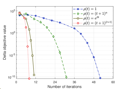
In Figure 1, the performance of the Spice method for single-variable QCQP problems is evaluated. In subplot (a), we show the objective function value versus the number of iterations. The different curve legends represent four different settings of the function: , , , and . The curves show a steady decrease in the objective function values as the number of iterations increases, with converging faster than the others, particularly within the first 10 iterations. The other settings for demonstrate a slower but consistent convergence behavior. Subplot (b) indicates the delta objective value, plotted on a logarithmic scale, which provides more insight into the convergence rate. Again, demonstrates a quicker decline in the delta objective value, indicating faster convergence. The results show that the choice of significantly impacts the convergence rate, with more aggressive functions leading to faster reductions in both the objective and delta objective values.
In Figure 2, the Spice method’s performance is extended to separable-variable QCQP problems. Subplot (a) shows the objective function values across iterations, where the same functions are used. As expected, exhibits the fastest convergence, closely followed by , while the constant function leads to a much slower decrease in the objective value. Subplot (b) shows the delta objective value on a logarithmic scale, revealing a similar trend where outperforms the others in reducing the objective error more rapidly. The overall conclusion from these figures is that the adaptive choices for can significantly accelerate convergence, with functions that grow with iterations providing more efficient performance in both single-variable and separable-variable QCQP problems.
| Dimensions | Single-variable QCQP | Separable-variable QCQP | ||||||||||
| p | PC | Spice: | Spice: | PC | Spice: | Spice: | ||||||
| 100 | 100 | 10 | 546 | 31 | 8 | 836 | 33 | 8 | ||||
| 300 | 300 | 10 | 12462 | 49 | 10 | 24068 | 53 | 10 | ||||
| 100 | 100 | 20 | 745 | 32 | 8 | 1129 | 35 | 9 | ||||
| 300 | 300 | 20 | 16890 | 51 | 10 | 33206 | 54 | 11 | ||||
Table 2 compares the number of iterations required by the PC method and the Spice method for both single-variable and separable-variable QCQP problems across different problem dimensions. The dimensions , , and refer to the problem size, with larger values representing more complex instances. For single-variable QCQP problems, the PC method consistently requires a significantly larger number of iterations than the Spice method, regardless of the function used. When , the number of iterations needed by the Spice method is greatly reduced, and when , the iteration count decreases even further. For instance, in the case where , , and , the PC method requires 546 iterations, while the Spice method with only takes 8 iterations, demonstrating the significant improvement in efficiency. Similarly, for separable-variable QCQP problems, the Spice method outperforms the PC method regarding the number of iterations. The trend persists as the problem dimensions increase, with the Spice method maintaining a more efficient convergence pattern, particularly with the function. For example, in the case of , , and , the PC method requires 33,206 iterations, whereas the Spice method with converges in just 11 iterations. This highlights the dramatic improvement in scalability offered by the Spice method with adaptive . This table illustrates the superior convergence performance of the Spice method, especially when utilizing the exponential function, which achieves faster convergence and reduces the number of iterations by several orders of magnitude compared to the PC method.
6 Conclusion
This paper introduced a novel scaling technique to adjust the weights of the objective and constraint functions. Based on this technique, the Spice method was designed to achieve a free convergence rate, addressing limitations inherent in traditional PC approaches. Additionally, the Spice method was extended to handle separable-variable nonlinear convex problems. Theoretical analysis, supported by numerical experiments, demonstrated that varying the scaling factors for the objective and constraint functions results in flexible convergence rates. These findings underscore the practical efficacy of the Spice method, providing a robust framework for solving a wider range of nonlinear convex optimization problems.
References
- [1] K. J. Arrow, L. Hurwicz, H. Uzawa, Studies in linear and nonlinear programming, Stanford University Press, Stanford, 1958.
- [2] M. Zhu, T. F. Chan, An efficient primal-dual hybrid gradient algorithm for total variation image restoration, in: UCLA CAM Report Series, Los Angeles, CA, 2008, p. 08–34.
- [3] B. He, S. Xu, X. Yuan, On convergence of the Arrow–Hurwicz method for saddle point problems, J. Math. Imaging Vis. 64 (6) (2022) 662–671. doi:10.1007/s10851-022-01089-9.
- [4] A. Nedić, A. Ozdaglar, Subgradient methods for saddle-point problems, J. Optimiz. Theory App. 142 (1) (2009) 205–228. doi:10.1007/s10957-009-9522-7.
- [5] J. Rasch, A. Chambolle, Inexact first-order primal-dual algorithms, Comput. Optim. Appl. 76 (2) (2020) 381–430. doi:10.1007/s10589-020-00186-y.
- [6] A. Chambolle, T. Pock, A first-order primal-dual algorithm for convex problems with applications to imaging, J. Math. Imaging Vis. 40 (1) (2011) 120–145. doi:10.1007/s10851-010-0251-1.
- [7] A. Chambolle, T. Pock, On the ergodic convergence rates of a first-order primal-dual algorithm, Math. Program. 159 (1) (2016) 253–287. doi:10.1007/s10107-015-0957-3.
- [8] T. Valkonen, A primal-dual hybrid gradient method for nonlinear operators with applications to MRI, Inverse Probl. 30 (5) (May 2014). doi:10.1088/0266-5611/30/5/055012.
- [9] Y. Gao, W. Zhang, An alternative extrapolation scheme of PDHGM for saddle point problem with nonlinear function, Comput. Optim. Appl. 85 (1) (2023) 263–291. doi:10.1007/s10589-023-00453-8.
- [10] X. Cai, G. Gu, B. He, X. Yuan, A proximal point algorithm revisit on the alternating direction method of multipliers, Science China Mathematics 56 (10) (2013) 2179–2186. doi:10.1007/s11425-013-4683-0.
- [11] G. Gu, B. He, X. Yuan, Customized proximal point algorithms for linearly constrained convex minimization and saddle-point problems: A unified approach, Comput. Optim. Appl. 59 (1) (2014) 135–161. doi:10.1007/s10589-013-9616-x.
- [12] B. He, X. Yuan, W. Zhang, A customized proximal point algorithm for convex minimization with linear constraints, Comput. Optim. Appl. 56 (3) (2013) 559–572. doi:10.1007/s10589-013-9564-5.
- [13] H.-M. Chen, X.-J. Cai, L.-L. Xu, Approximate customized proximal point algorithms for separable convex optimization, J. Oper. Res. Soc. China 11 (2) (2023) 383–408. doi:10.1007/s40305-022-00412-w.
- [14] B. Jiang, Z. Peng, K. Deng, Two new customized proximal point algorithms without relaxation for linearly constrained convex optimization, Bull. Iranian Math. Soc. 46 (3) (2020) 865–892. doi:10.1007/s41980-019-00298-0.
- [15] B. He, PPA-like contraction methods for convex optimization: A framework using variational inequality approach, J. Oper. Res. Soc. China 3 (4) (2015) 391–420. doi:10.1007/s40305-015-0108-9.
- [16] B. He, F. Ma, X. Yuan, An algorithmic framework of generalized primal-dual hybrid gradient methods for saddle point problems, J. Math. Imaging Vis. 58 (2) (2017) 279–293. doi:10.1007/s10851-017-0709-5.
- [17] S. Wang, Y. Gong, Nonlinear convex optimization: From relaxed proximal point algorithm to prediction correction method, Optimization, under review (2024).
- [18] S. Wang, Y. Gong, A generalized primal-dual correction method for saddle-point problems with the nonlinear coupling operator, Int. J. Control Autom. Syst., accepted (2024).
- [19] B. He, F. Ma, S. Xu, X. Yuan, A generalized primal-dual algorithm with improved convergence condition for saddle point problems, SIAM J. Imaging Sci. 15 (3) (2022) 1157–1183. doi:10.1137/21M1453463.