SPICE PSF Correction: General Framework and Capability Demonstration
We present a new method of removing PSF artifacts and improving the resolution of multidimensional data sources including imagers and spectrographs. Rather than deconvolution, which is translationally invariant, this method is based on sparse matrix solvers. This allows it to be applied to spatially varying PSFs and also to combining observations from instruments with radically different spatial, spectral, or thermal response functions (e.g., SDO/AIA and RHESSI). It was developed to correct PSF artifacts in Solar Orbiter SPICE, so the motivation, presentation of the method, and the results revolve around that application. However, it can also be used as a more robust (e.g., WRT a varying PSFs) alternative to deconvolution of 2D image data and similar problems, and is relevant to more general linear inversion problems.
Key Words.:
¡ line: profiles - techniques: imaging spectroscopy - instrumentation: spectrographs - techniques: high angular resolution - Sun: abundances - Sun: corona ¿1 Introduction
SPICE (Spectral Imaging of the Coronal Environment, Spice Consortium et al., 2020) is an EUV slit scanning spectrograph on board the Solar Orbiter spacecraft (García Marirrodriga et al., 2021). It has a arcsecond per pixel spatial plate scale along the slit and several slit widths ranging from 2 to 30 arcseconds, while the spectral plate scale is nm per pixel. The focal plane has two detector arrays of pixels each, covering two spectral bands – one from 70.4 to 79.0 nm and the other from 97.3 to 104.9 nm. The slit scanning mechanism can cover up to 16 arcminutes, while the slit covers 14 arcminutes on the detector plane. The overall raster image dimensions are up to arcseconds. SPICE’s observing distance varies between about 0.3 and 1.0 AU, which must be considered when comparing these numbers with Earth-based instruments.
A primary design objective of SPICE is tracing the connectedness of the photosphere and low corona out to the heliosphere – primarily by connecting abundances observed in situ by various spacecraft with those sensed remotely by SPICE. This relies on accurate identification of particular emission lines at a variety of temperatures; lines which have varying susceptibility to ionization (the FIP, or First Ionization Potential, effect) (see Spice Consortium et al., 2020, for more detail). An additional important feature of SPICE for diagnosing connectedness is the use of the Doppler effect to discriminate upflows from downflows and to identify potential solar wind outflow regions deep in the corona and transition region.
Although SPICE is not a high resolution instrument by design, these and other observables, along with their driving science objectives, require reasonable resolution within the limits of its design (given the mission’s nominal requirements; see Spice Consortium et al., 2020); degraded resolution beyond the design limits will impact the ability to achieve SPICE’s science goals. This paper reports on some issues that degrade SPICE’s resolution, and a novel data processing methodology which will remove the degradation.
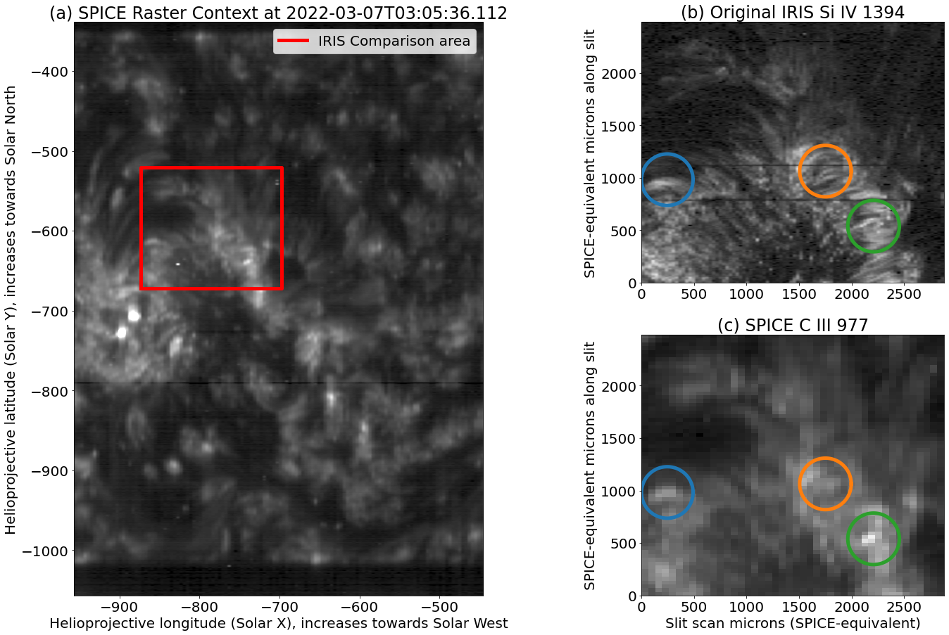
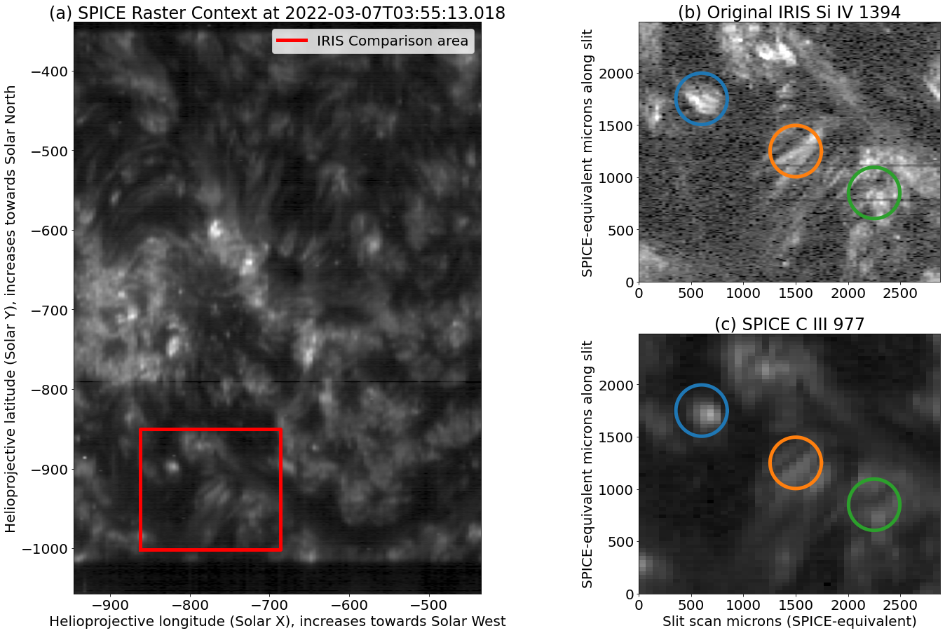
We will be using a set of coordinated SPICE and high spectral and spatial resolution IRIS (Interface Region Imaging Spectrograph De Pontieu et al., 2014) data for the examples and demonstrations in this paper, with IRIS data used as ‘ground truth’ to assess the quality of the deconvolution and constrain the effective SPICE PSF. The observations were taken on March 7, 2022, when SPICE’s orbit placed it on the Earth-Sun line, with the same perspective as IRIS. We will compare the SPICE C III 977 Å observations with IRIS Si IV 1394 Å observations; These two lines form very close in terms of temperature, at log T [K] of 4.78 and 4.81 in ionisation equilibrium (e.g., Table 1 of Peter et al., 2006). An image showing the larger context of this region is shown in Figure 1.
2 Overview of SPICE PSF Problem and Possible Solution
2.1 PSF Issues and need for correction
Since SPICE is a scanning slit spectrograph, its observables are in three dimensions – spectral (), slit-aligned (), and slit-perpendicular (, the scanning direction; actually, there is a fourth time dimension but we do not consider this here because we assume the source and PSF do not change with time). The SPICE PSF is similarly three-dimensional, extending in all three of these directions. The issue this paper addresses is caused by a PSF that is both elongated and rotated with respect to these axes, rather than being aligned with them. We have observed that the SPICE PSF is rotated both within the slit plane (i.e., ) and in some cases in the scanning plane as well. This is shown for an example slit plane by Figure 2; this slit plane passes through the middle of the green circled region in Figure 1. A rotation on the detector (i.e., ) plane of is evident (this angle will appear different if the pixels are not square, and can vary with the different slit width; this paper focuses on the 2 arcsecond slit). We believe this issue is caused by a combination of astigmatism on the primary mirror and defocus.
This elongation and rotation of the SPICE spectro-spatial PSF impacts its ability to diagnose connectedness and other important instrument capabilities in a variety of ways. It reduces the definition with which SPICE can resolve boundaries of regions with differing connectedness – some of these can be rather small and in general small changes in the region identification can result in large impacts on the quality of the association with in situ observations. The degradation also hampers the ability to resolve the fainter spectral lines when there are neighboring bright spectral lines. This is especially critical because the selection of lines which adequately sample both abundance and temperature is very limited (the aforementioned spectral blends are a case in point).
Even more challenging is that the tilt of the PSF between that spatial and spectral directions causes a bright feature at one location to create the illusion of a neighboring dim feature, which is Doppler shifted relative to the true feature – i.e., bright features appear to have Doppler shift lobes next to them; Together with Doppler fitting, the elongated and rotated ‘effective PSF in the plane acts like an edge detection filter, causing bright features to be ‘aliased’ from intensity into Doppler (As previously mentioned, we believe this issue is ultimately caused by a combination of astigmatism on the primary mirror and defocus). This confounds attempts to understand connectedness and dynamics by looking at Doppler shifts, and we have seen this kind of feature in the SPICE data.
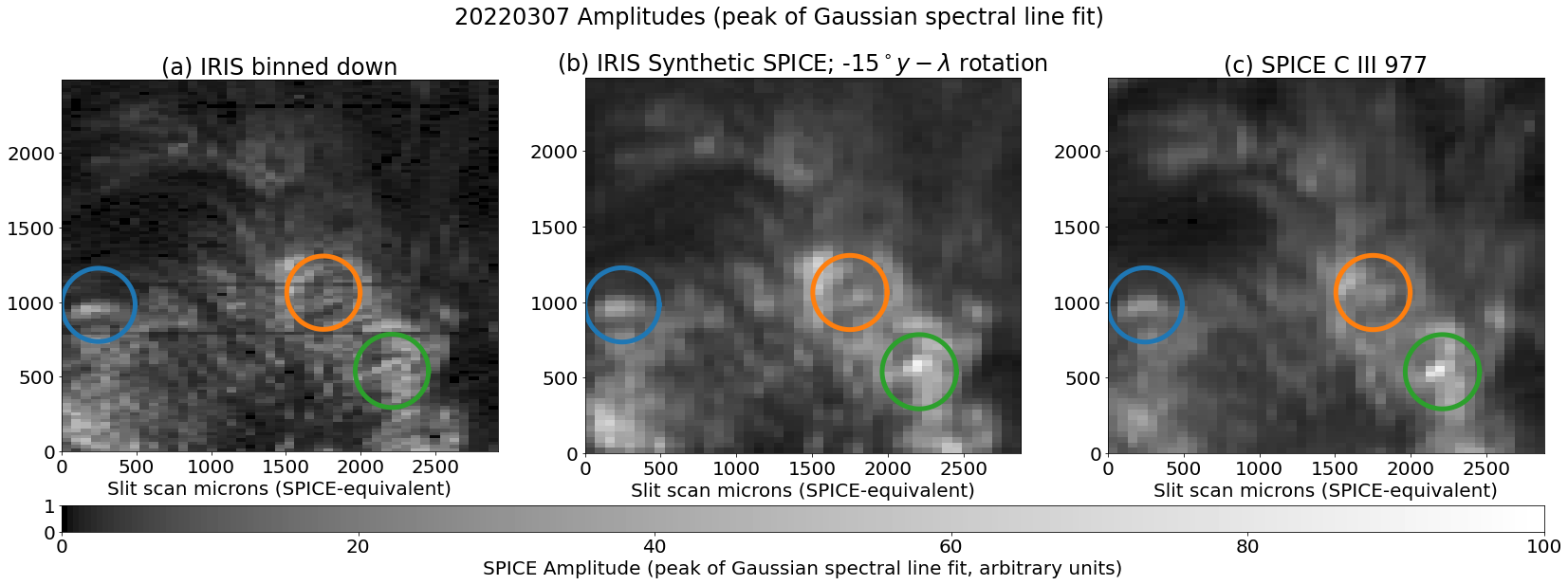
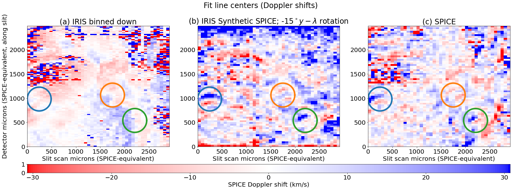
To illustrate the issue, we show (in the lower panels of Figure 3) the Doppler fits to the binned down IRIS data, the IRIS data degraded with the SPICE PSF, and the actual SPICE data, for the region of interest already highlighted by Figure 1. Strong Doppler features are evident in the IRIS data degraded with SPICE PSF and the SPICE data which are not present in the original IRIS data. We have circled three of the most prominent such features in the Doppler map. Each of these coincide with bright features (e.g., ridges) in intensity, as can be seenin the lower panels of Figure 3. The clear appearance of the same features in IRIS with the SPICE PSF, when they are absent from the original (plus down-binning) IRIS data, clearly implicates the PSF in creating these artifacts. A similar effect and artifacts have been previously noted for Hinode EIS (Culhane et al., 2007). This is primarily discussed in an online EIS SW note (Ugarte-Urra, 2016), but also alluded to in other papers such as Young et al. (2012).
2.2 Solution method: general linear (sparse) solvers and why we’re using them
These examples suffice to illustrate that this PSF effect seriously degrades the quality of Doppler data observed by SPICE. A means of removing it is highly desireable, and the objective of this work is to develop such a method which could ultimately be applied to all data at some level of its data pipeline. The conventional way of removing PSFs is via convolution (e.g., Poduval et al., 2013). Convolution in this context is the translationally invariant special case of the general linear transform, and usually also assumes that the input and output of the transform have the same dimensions (e.g., by pixels). Rather than treat the problem under this special case, however, we instead treat it as an example of the full general linear transform. There are a number of reasons for this choice, including:
-
•
Pragmatically, we expect these PSF artifacts to vary over the image plane, Which a convolution cannot represent;
- •
-
•
The general full linear problem is far more broadly applicable than the (de)convolution problem. Once properly developed, the same tools used for this problem with SPICE can be applied to almost every other coronal remote sensing problem, to similarly good effect. See Plowman (2021) for an early example. We will return to this point at the end of the paper.
-
•
The tools for tackling the inverse part of this problem have already been extensively developed by the computer science communities, in the form of high performance sparse matrix solvers. All we need to do, therefore, is implement the forward transform in the appropriate fashion, i.e., as a sparse matrix.
We turn next to our implementation of this method. The derivation shown next presupposes a 3D PSF as a function of , , and (the most general case for SPICE). In practice, our understanding of the problem is that it can be represented by two PSFs. The first blurs in and but does not affect . Therefore, this PSF does not contribute to the Doppler artifacts we are trying to correct. The other ‘effective’ PSF is assumed to affect and but not . This is the PSF that is elongated in and rotated , and which causes the Doppler artifacts. We have done a variety of tests with 2D and 3D PSFs, and found that correcting this effective PSF suffices to remove the Doppler artifacts, working as well as the 3D correction while being much faster. We leave the derivation presented here in 3D because it is more general and was already written that way. The code for doing the correction is written to be agnostic to the dimensionality of the problem, as the supplementary 1D and 2D examples demonstrate.
3 Introducing our solution method (Formalism)
3.1 SPICE PSF as instance of general linear forward problem
3.1.1 The SPICE forward problem
To begin, let us suppose SPICE observes some static (meaning it does not change over the time of observation) cube on the sky, with spectral radiance as a function of sky longitude and latitude (which we will write as ) and wavelength . These are projected onto the detector plane by the PSF, , which is a function of both sky coordinates () and detector plane coordinates (). In reality, and are time-multiplexed onto the same surface (although not necessarily the same axis) by the grating, slit, and scanning mechanism, but we will treat them as independent for clarity of demonstration. The flux density on the detector plane observed for this cube is the integral of the cube against the PSF over all sky angles:
| (1) |
Where we have made the small angle approximation and placed the Sun at the equator of the coordinate system which allows us to set the weight in the integral to one. The sensors divide the detector plane into pixels which we will index by and , each of which have weight functions (typically non-overlapping ‘bins’) . The fluxes into each of these pixels are the integrals of the detector plane flux densities against each of these weight functions:
| (2) |
At this point we point out what we call the overall response function of the th pixel of the instrument,
| (3) |
The name of the game is to find the spectral radiance, , which is an unknown continuous function and therefore has an infinite number of degrees of freedom. To limit the number of degrees of freedom we can without loss of generality (in practice if not in principal) define in terms of a linear combination of a set of appropriately chosen basis functions, :
| (4) |
where are the coefficients of the linear combination. The basis function set ought to be linearly independent (i.e., no basis function can be expressed as a linear combination of the others). It is useful for the present purpose if each one is spatially compact and does not overlap much (or at all) with the other basis functions. They should also cover the sky plane at least as well as the pixels cover the detector plane. A set of pixel like ‘bins’ in with equivalent (or denser) spacing to the pixels will suffice and is the choice we use in this paper. The indices are intended to reflect the identification of the bins with the coordinate axes. In terms of this, the pixel fluxes are
| (5) |
If we recognize an array of response coupling terms,
| (6) |
(the consituents of this are all known and computable, being composed of the basis functions and the in principal known instrument response functions) we are left with the following linear equation relating the unknowns () to the knowns ():
| (7) |
We have used three indices each for the coefficients and the observables, but this is simply a notational convenience that allows us to identify each of the coordinate axes with its own index. Mathematically, we can ‘flatten’ all these indices down to a pair of indices (one for the coefficients, and one for the observables) by relabeling according to the following one-to-one correspondence:
| (8) |
| (9) |
Our linear equation then becomes
| (10) |
Which we recognize as a familiar matrix equation, with the array of coupling terms becoming a forward response matrix. Any N-dimensional linear discrete or integral transform can be similarly treated, and nonlinear ones may be amenable to a linearization and iteration approach, so this can be a very powerful and general method for dealing with these problems.
3.1.2 1D and 2D Examples
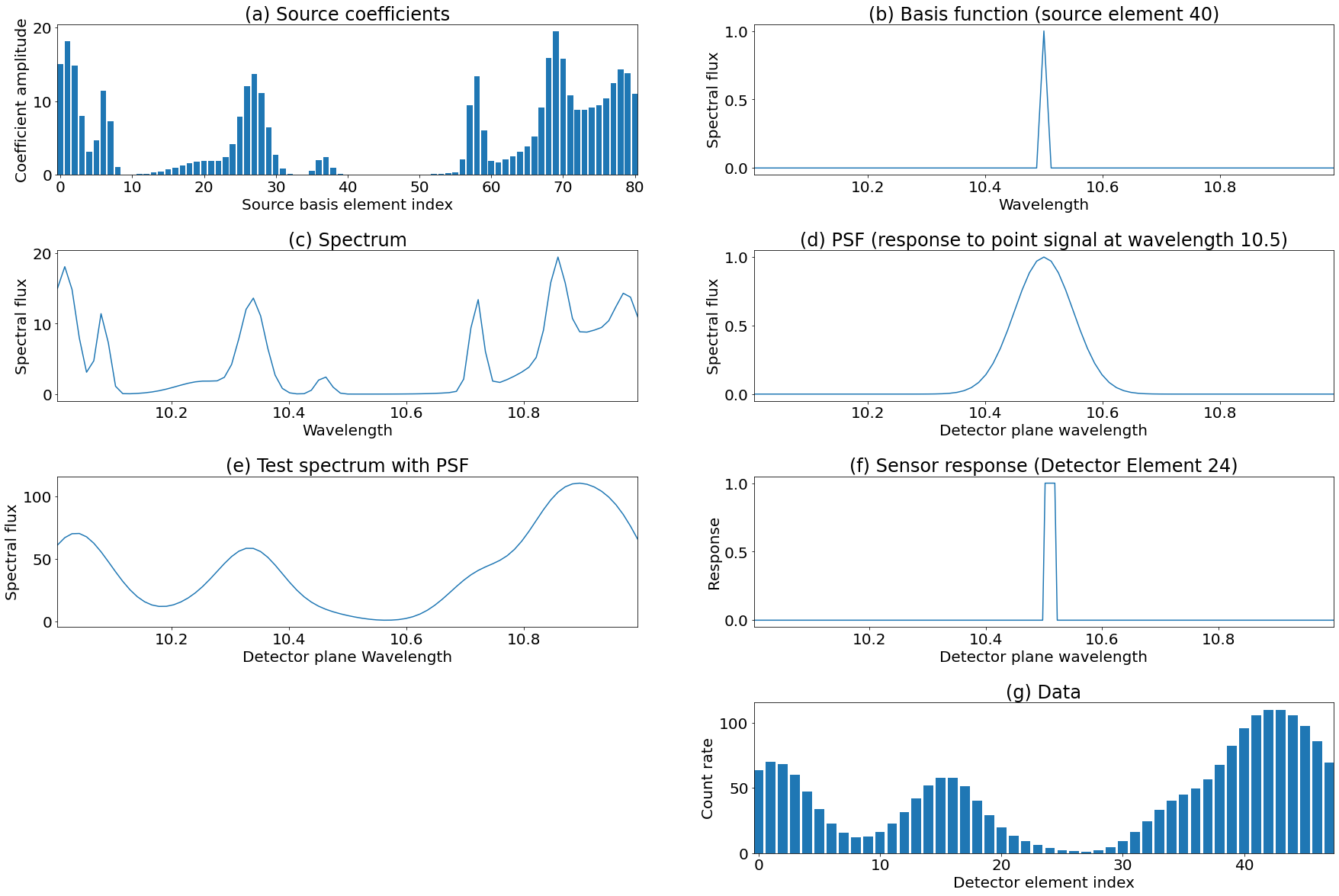
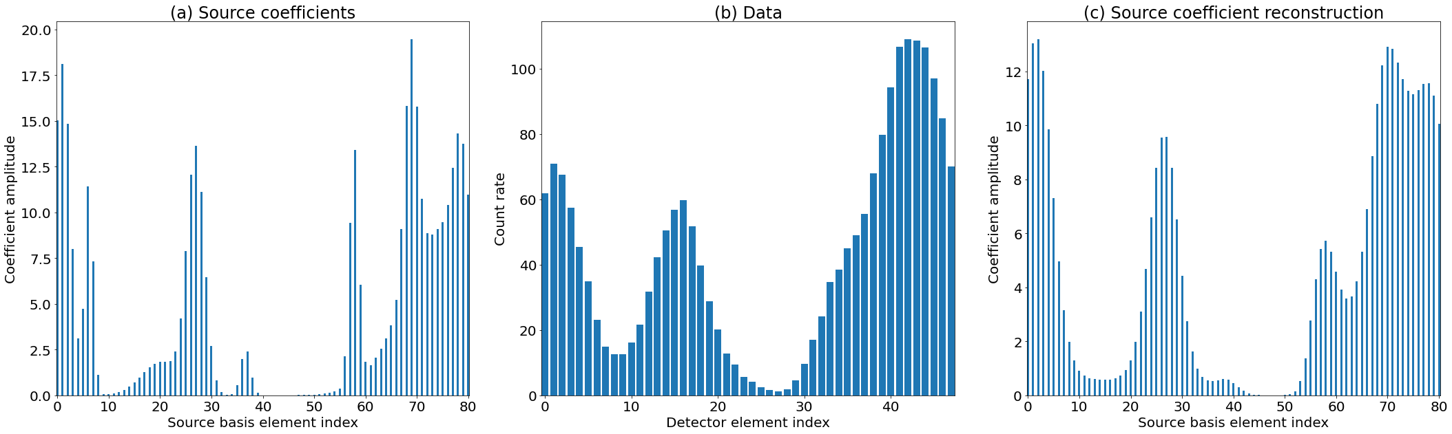
At this point, a pair of lower dimensional examples may be illustrative. Consider the spectrum for a single pixel, i.e., a function only of (for example) wavelength. This is equivalent to the DEM problem as presented by Plowman & Caspi (2020), the only difference being that instead of the instrument temperature response functions found there, we have a combination of the wavelength PSF and pixel bin functions:
| (11) |
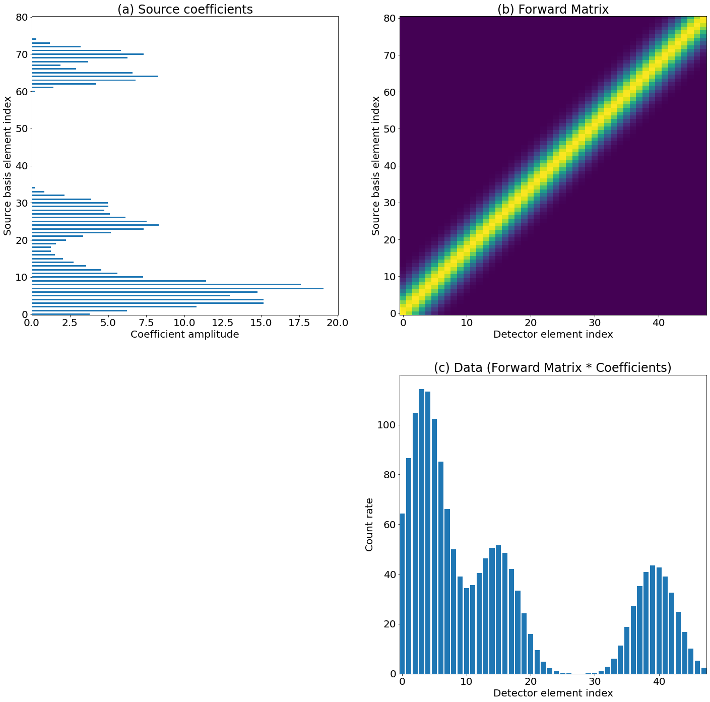
The forward matrix is
| (12) |
This is illustrated graphically in Figures 4 and 5. The only difference between them is that in Figure 4, the individual steps are depicted, whereas Figure 5 combines all of these steps into the forward matrix – This is possible because all of the individual steps are linear operations.
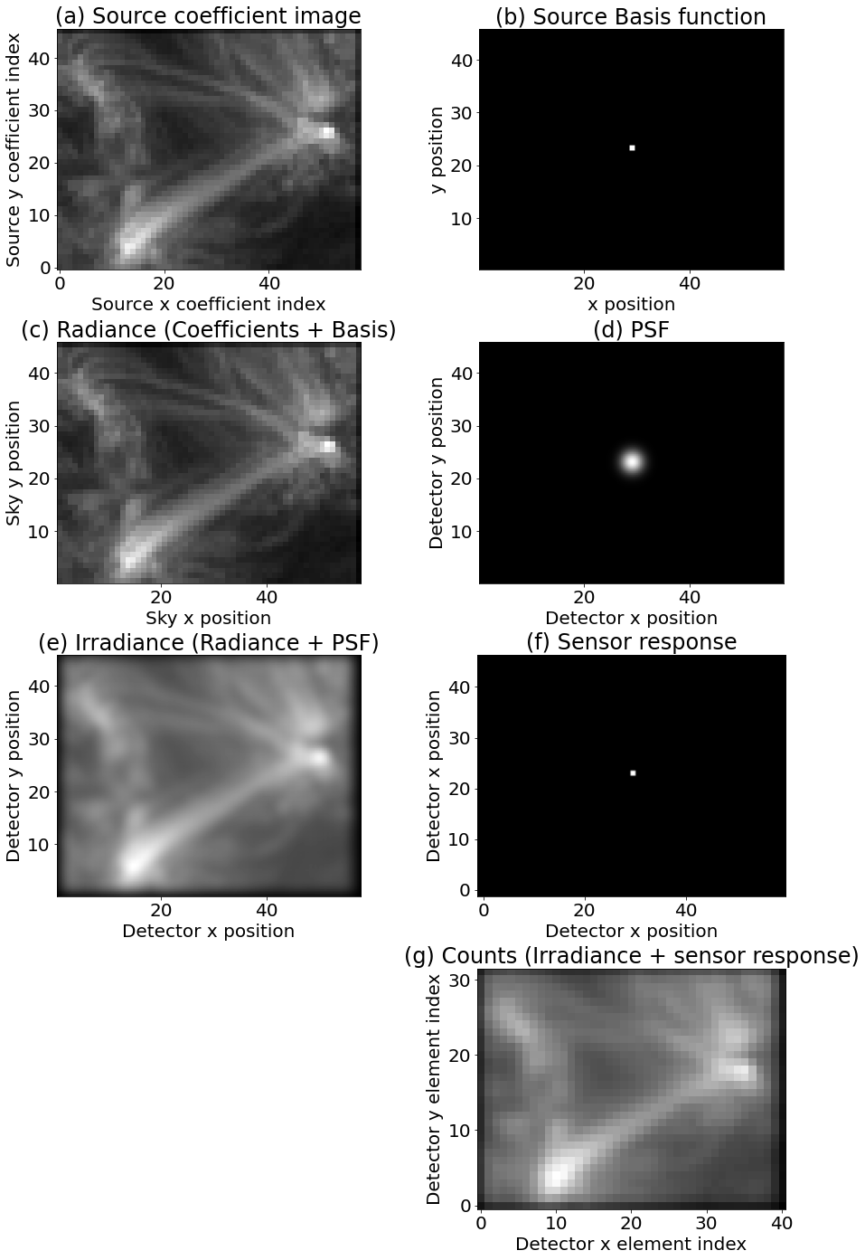
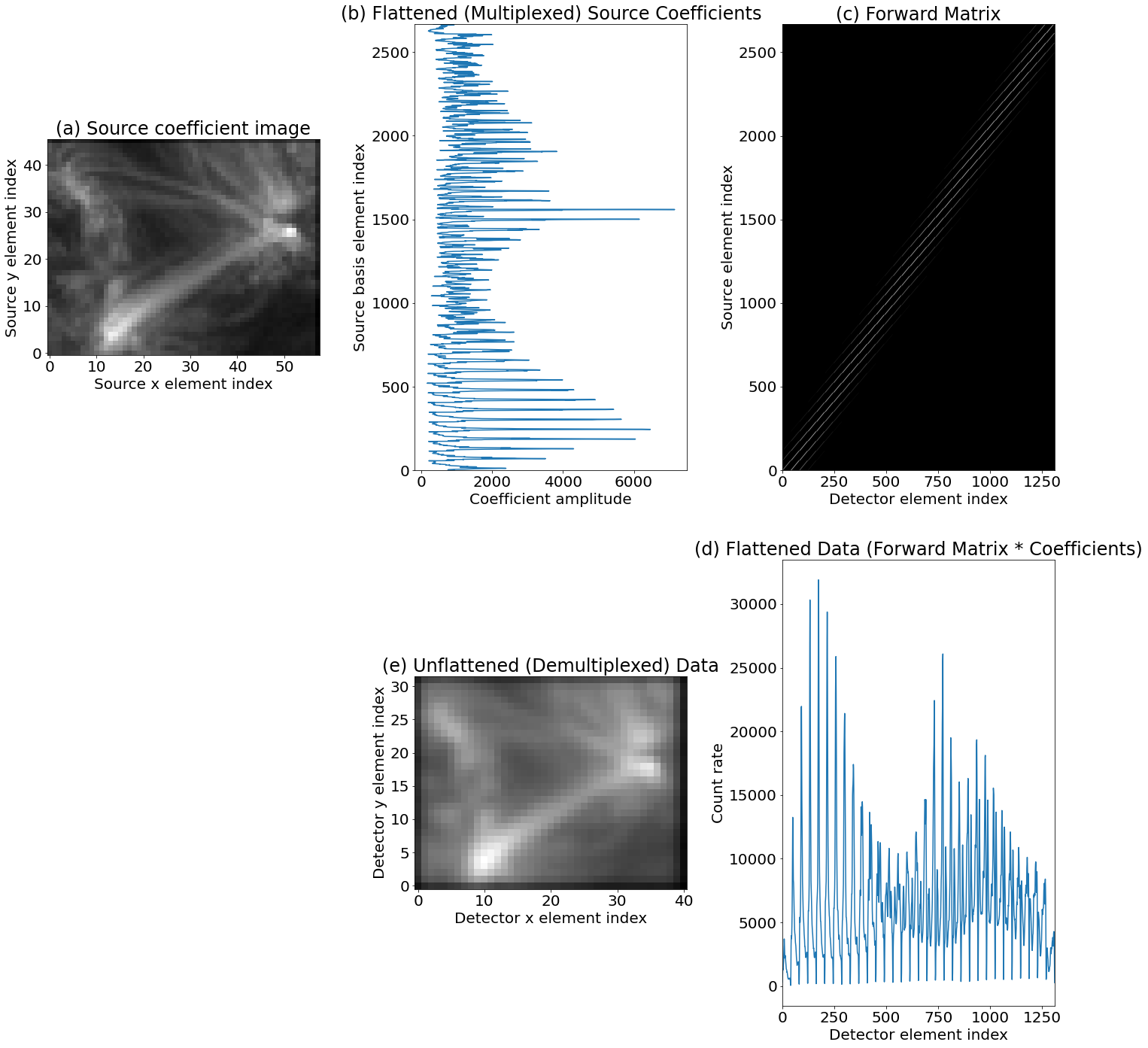
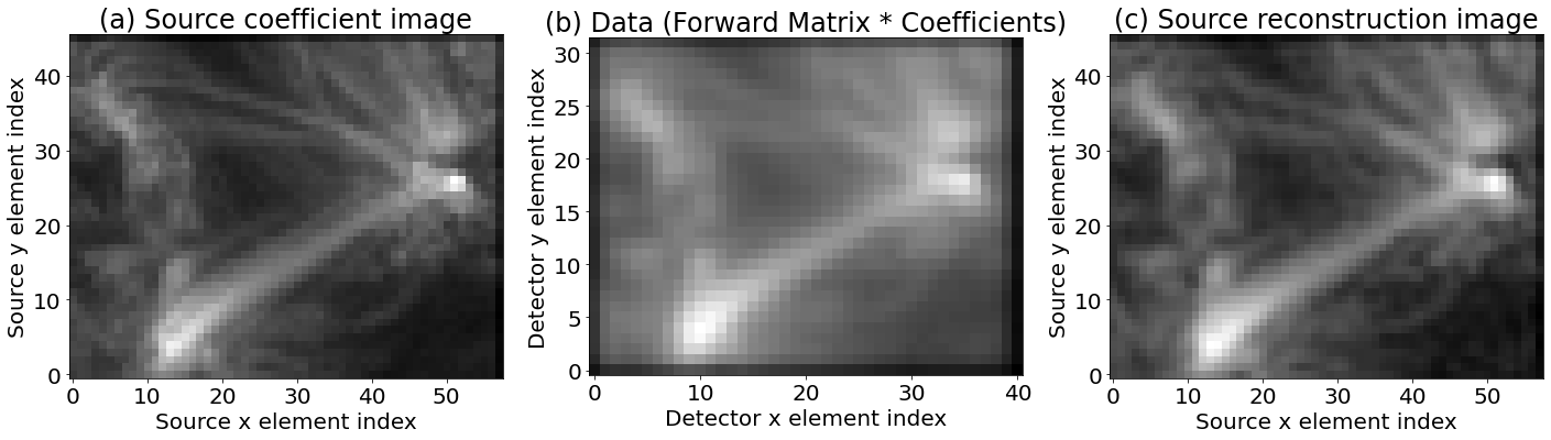
Figures 6 and 7 are of the same format and show how the same treatment can be scaled up to two dimensions (spatial, in this example, although it makes no difference in the mathematical treatment). Essentially, the additional dimension in the source and the detector are simply multiplexed down to the one ‘input’ (conventionally the columns) and one ‘output’ dimension of the forward matrix. Mathematically, the only difference is the addition of a multiplexing (e.g. by ‘flattening’ in numpy or reforming to a 1D vector in IDL) step at the beginning and, if desired, a demultiplexing step at the end (e.g., by using reform in IDL or reshape in numpy) – But these are trivial 1-to-1 operations. This additional multiplexing step is shown in the top left and bottom center panels of Figure 7, which otherwise is identical in format to the one-dimensional figure (5). The output resolution of these examples differs from the input, because in general the resolution of solar sources differs than that of our detectors, to demonstrate that this framework can accomodate such resolution differences.
The SPICE forward problem for the effective () PSF is equivalent to this 2D correction, while the full forward problem follows the same trend from 1D to 2D to 3D – the same multiplexing and demultiplexing operations suffice to convert the problem into matrix form. The practical implementation of this can be conceptually thorny, but we have developed a general N-Dimensional, coordinate aware framework in Python for computing these matrices. This will be described in more detail in Section 3.4, and the framework is also available for download (see Section 3.4).
3.1.3 Sparse Matrix Algorithms
It is clear from the examples provided above that the forward matrix is very large, even for images of modest size. However, only detector elements within PSF range of the source elements have non-zero entries, and the PSF is much smaller than the overall image. Therefore, this matrix is sparse. A wide variety of specialized sparse matrix algorithms exist to work with such matrices and they drastically reduce the real-world memory and processing requirements of working with these matrices. Standard examples can be found in, for instance, Press et al. (2002). Additionally, solving linear problems based on sparse matrices is well developed field in computer science, and by casting the problem in this form we can avail ourselves of the tools that have been developed. Our framework for computing the forward matrices is built on these algorithms, specifically making use of the scipy.sparse sparse matrix package.
3.2 Solving the SPICE forward problem
The fundamentals of this solution method have also been recently discussed in Plowman & Caspi (2020); Plowman (2021), but we will also cover them here to show how they apply to this case. We begin by considering the forward problem in the linear least squares framework (Press et al., 2002):
We seek to find the ‘best fit’ coefficient vector ( in Equation 10) that minimizes the sum of squares (hence, the ‘least squares’) of the deviation of our model prediction for the data – from Equation 10 – with the data, . These squared deviations are weighted by the inverse of the square of the errors in the data, . This weighted sum is also known as a statistic:
| (13) |
The above assumes that the errors in the data are normally distributed, which can be seen by noting that in that case the log likelihood is . Because this merit function is convex, it has only one minimum which occurs where the gradient of with respect to the coefficient vector is zero. Better yet, because is quadratic, its derivative is linear. The best fit coefficient vector is therefore found by solving the following matrix equation (cf. the chapter in Press et al., 2002, on Linear Least Squares):
| (14) |
Where
| (15) |
This is the standard form for matrix problems in linear algebra, and in principle the linear least squares best fit solution is
| (16) |
Reality is never quite so simple, of course – we need to apply some additional constraints to ensure a well-posed solution, which we discuss next.
3.3 Positivity Constraint and Regularization
The matrix is likely to be poorly conditioned even if it is not outright singular. The blurring caused by the PSF means that details we would like to resolve are degraded by the forward transform – it loses information – even if the number of data points is equal to the number of coefficients; in this case, will be poorly conditioned, and detector noise will lead to instabilities in the reconstruction. If the number of data points is less than the number of coefficients, then will be singular and simply inverting Equation 14 will not be possible. To resolve this issue, we apply a positivity constraint and regularization.
3.3.1 Regularization
Regularization typically takes the form of an additional term to minimize which is added to . In this derivation, we will take this to be of the form
| (17) |
In other words, instead of minimizing by itself, we seek to minimize the merit function
| (18) |
Where is a matrix specifying the regularization. This can be as simple as the identity matrix, in which case the regularization makes the solver prefer solutions with a smaller norm (i.e., ). Exactly how much smaller depends on the size of the parameter, which tunes the strength of the regularization. In Plowman & Caspi (2020), the operator was composed of the derivatives (WRT temperature, in that case) of the basis functions integrated against each of the other basis functions. This results in a regularization operator that makes the solver prefer solutions with the smaller derivatives – specifically the log of the derivative in that case.
The addition of the regularization term changes the matrix equation we wish to solve from Equation 14 to
| (19) |
In other words, the matrix that needs to be inverted simply has the regularization matrix times the tunable paramater () added to it.
For this class of problem, is often chosen to make each the residuals of the fit to be some number (typically equal to the number of data points, or ‘reduced’ of order unity). Noting that the residuals are , and with a slight rearrangment of Equation 19, this requirement is equivalent to
| (20) |
We want to solve this for . But this is just one parameter and can’t satisfy each component of this vector equation. Instead, minimize the RMS of the LHS of this equation over lambda. The result is
| (21) |
But we don’t know , either. We therefore use an initial guess for to determining our . We’ll need one later on when we introduce the positivity constraint, anyway.
It turns out that a simple initial guess can be formed using . An analogy can be made to upscaling an image by an integer factor. More generally, the results of this procedure are roughly a model which has been subjected to the source response function twice. It will be much smoother, but features will be in the right place. This is desirable for regularization and it is more conservative and therefore avoids overfitting. It does result in an over-smoothed solution as well, however, the amount of which depends on how much sharper the source is than the results of the instrument resolution degradation. To mitigate this, we apply a final correction factor to . The SPICE sources are significantly sharper than the SPICE PSF, so the used is about 0.1.
The amplitude needs to be rescaled (since is not normalized). We choose this scaling factor to be the one that minimizes the of this initial guess compared with the data, resulting in the following initial guess for :
| (22) |
The framework as currently constructed uses regularization based the norm. The derivative-based regularization used in Plowman & Caspi (2020) could also be done here, but it would require constructing gradient operator matrices with respect to image position and wavelength, which is doable but too involved to include in the present publication. It will be implemented in future work, however, which will open up a variety of possibilities for including more physical constraints on inversions using this framework, as well as some other intrinsic benefits.
3.3.2 Positivity Constraint: nonlinear mapping
One condition that the sources of these data must satisfy is positivity: spectral radiances cannot be negative. This is a nonlinear constraint, which can’t be directly captured by a linear formalism. Instead, we use the same nonlinear mapping on the coefficients as in Plowman & Caspi (2020). We express in terms of a second set of parameters, , such that
| (23) |
We then choose the mapping function, , to be one whose range is limited to the non-negative numbers. Two such examples are and ; we use the former (exponential) mapping here, as it seems to produce better convergence properties. We then linearize and iterate beginning from an initial guess. The results of this are described in more detail in Plowman & Caspi (2020), and we will not repeat all of the steps of the derivation here although we have changed the notation somewhat in an attempt at better clarity. The one difference is that in Plowman & Caspi (2020) only the case where the regularization acts on the , rather than the was considered. If the regularization acts on the instead, there are additional terms (shown below).
The result is the following matrix equation
| (24) |
| (25) |
and
| (26) | |||||
where is the mapping function for the regularization. It is equal to if the regularization is with respect to and if it is with respect to , and primes on or represent their derivatives with respect to their arguments. represents the coefficient parameters from the previous step of the iteration. There’s no reason the regularization couldn’t use some other mapping function of , but we do not further consider that possibility here; we use the same mapping for both and the regularization (). The regularization strength, , likewise changes to
| (27) |
These equations suffice to ensure positivity, which in addition to being required by the physics makes the solutions more well-posed in many situations. It does require an iteration, but the convergence is generally good provided the mapping functions are monotonic (this makes the overall optimization problem convex, so the figure of merit has a single global minimum).
3.3.3 Solvers: GMRes, Bicstab, etc
Since these matrices are very large, they require sparse solvers. These generally rely on some sort of iterative process in order to avoid dealing with the fully populated matrix. The code for applying these corrections is developed in Python, so we have been using the solver algorithms included in the sparse package of SciPy (Virtanen et al., 2020a). Specifically the stabilized biconjugate gradient (bicgstab van der Vorst, 1992) and lgmres (Baker et al., 2005) algorithms. Both of these algorithms have a long heritage – they are variants of algorithms mentioned in the 1992 edition of Press et al. (2002), namely the Biconjugate Gradient and Generalized Minimal Residual methods. We have tested both and found their convergence and performance to be comparable and more than acceptable for the problem at hand.
3.4 Implementation Details & Practical Considerations
To accompany this formalism, we have developed a flexible coordinate-aware Python framework which can compute basis functions, PSF, and response matrix for arbitrary source and detector dimensions. It contains the following components:
- Basis functions
-
Rectilinear N-Dimensional ‘bin’ and ‘triangle’ functions are provided as examples, and others can easily be added.
- Point Spread Functions
-
Functions specifying how an N-Dimensional detector plane is illuminated by a point source at a particular location. A Gaussian-based ‘boilerplate’ PSF is included as an example (see Section 3.4.1 below).
- Coordinate Grids
-
These represent the standard notion of an N-Dimensional array of coordinate points indexed to a grid. They are defined in terms of a coordinate system and a transform from grid indices to a set of coordinate points. The transform may be defined in terms of an origin (the location of the center of the element with all indices zero), a set of sizes (, , etc), and the dimensions of the array, but more complex transforms are also possible. This transform must be one-to-one.
- Source and Detector Element Grids
-
These represent the standard notion of a gridded array of elements, and can be either a set of source basis elements or detector elements (pixels). They are defined in terms of the coordinate grids and registered to it, but add code for returning the coordinates and amplitude of a particular basis element and for returning the response of all detector elements to a particular point source. Sources and detectors are independent and each have their own coordinate system.
- Coordinate Transform
-
A transformation from the coordinate system of the source model to the coordinate system of the detector. This is build to interface with the coordinate grids, and is also setup with the astropy (Astropy Collaboration et al., 2013a, 2018a) and sunpy (The SunPy Community et al., 2020a) coordinate systems in mind, but for these examples we use a trivial identity transform, leaving the source defined in terms of detector units, and registered to the same grid. This transform does not need to be one-to-one – e.g., it can map from a set of 3D spatial points on the sky to a 2D detector plane.
This framework should be able to accommodate detectors whose elements are not gridded in the usual way – RHESSI (Lin et al., 2002) could be an example of this – but we do not further explore the possibility in this paper. Likewise, we will leave detailed description of the framework to its codebase and example usage software, which will be made available along with the published paper.
3.4.1 ‘Boilerplate’ PSF Model
For the work shown next, we use a ‘Boilerplate’ model of the PSF which consists of a two component, 2D Gaussian where each component can be raised by an additional exponent to weight it more toward its wings or its core. We found that setting this exponent to made for a closer match between the IRIS line profiles (with our PSF added) and the SPICE line profiles, although the effect on the corrected Doppler shifts was very small. The mathematical expression for these Gaussians is:
| (28) |
where is the difference between the coordinate vector of the source and the coordinate vector on the image plane, e.g., in equation 1. is the covariance matrix of the Gaussian, and is the exponent (an exponent of one is a standard Gaussian). We specify this in terms of a set of initial axis lengths (the uncertainties of the principal axes without rotation) and rotation angles, in which case one begins with a diagonal covariance matrix that has the principal axis uncertainties on the diagonals and then rotates the matrix to its final position with a succession of rotation matrice(s) – one in the 2D case, 3 in the 3D case – Our implementation includes an example implementation of this PSF that works in both 2D and 3D.
4 Testing & Application
To begin, we show the method applied to the one and two-dimensional examples shown earlier. Figure 8 shows reconstruction of the example shown in Figure 4, while Figure 9 shows reconstruction of the example in Figure 6. In both cases, the reconstruction recovers most of the features of the source which are not evident in the data, despite the presence of PSF, noise, and (in the 2D example) a lower pixel resolution. Apparent noise is amplified by this process, but this is an inevitable consequence of the flow of information in this problem: below some threshold, noise and features cannot be distinguished.
4.1 Application to SPICE data and comparison with coordinated IRIS data
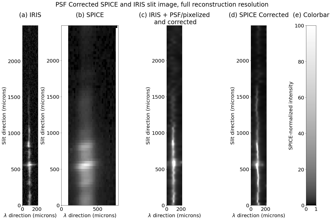
We now show application to the example SPICE data shown earlier. As previously mentioned, we are treating the overall SPICE spatio-spectral response function as an response function representing (primarily) the main (spatial focusing) mirror followed by a ‘effective’ response function representing the elements that contribute to the spectral PSF, including the grating, and final pixelization. To reduce the size of the inverse problem, this example incorporates the downsampling in , including a 2-pixel binning in that direction, into the response function. This is not strictly required, although it does also help to increase the SNR. The resolution change, of course, all happens as part of the response function.
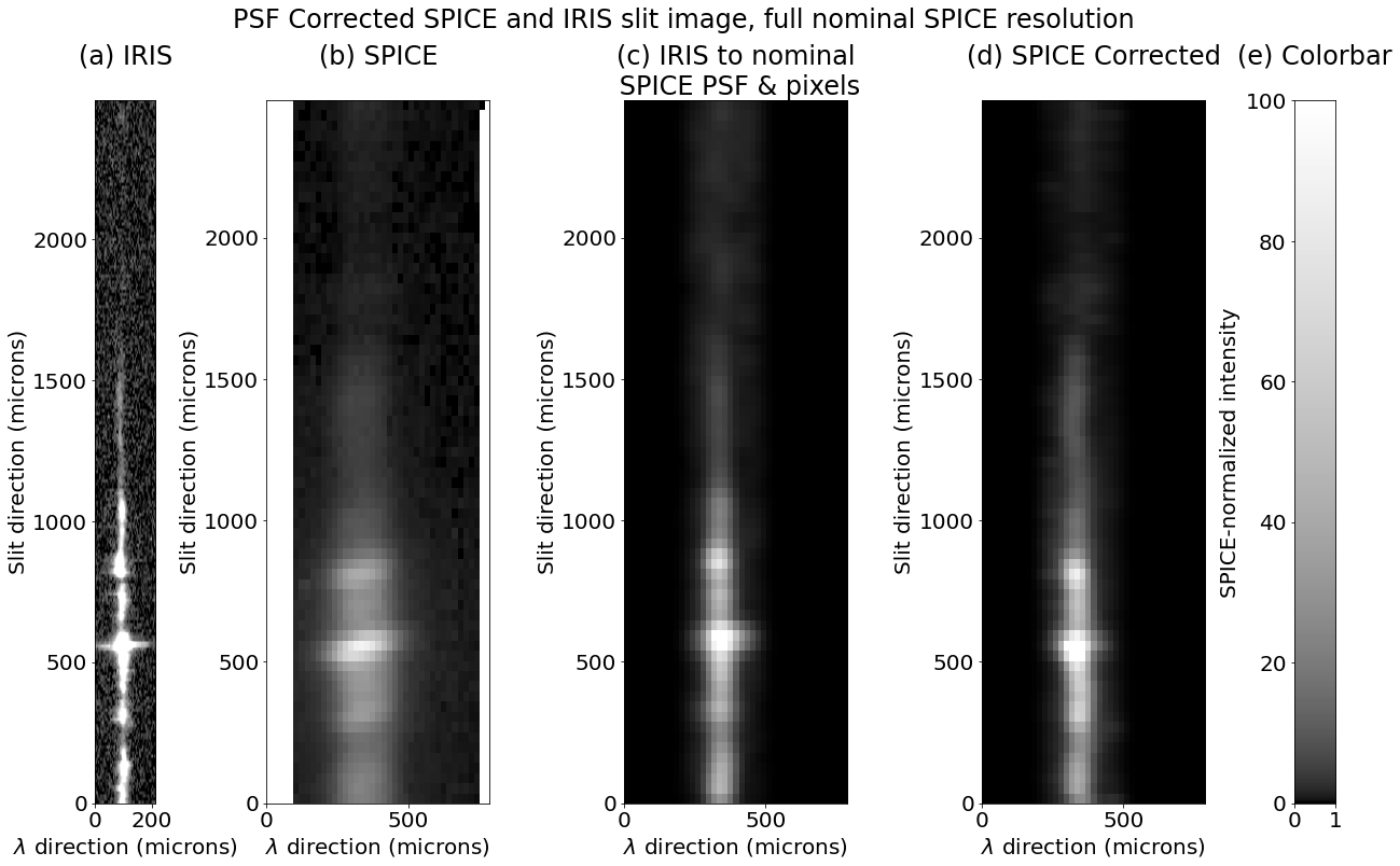
The correction uses the full IRIS resolution in ; even though this is considerably higher than the SPICE resolution, it is necessary to properly resolve the spectral line – The combination of positivity constraint, regularization, and the fact that the MTF of the PSF doesn’t completely go to zero means that the correction can somewhat exceed the standard Airy/Nyquist criteria, especially since the spectral direction is mostly composed of near zero-amplitude signal. This super resolution can result in some ringing and overfitting features due to noise, however, so we apply a new forward matrix that applies a ‘nominal’-sized SPICE PSF and returns the pixel scale to that of the original data. The size of this ‘nominal’ PSF is based on the resolutions described in the SPICE instrument paper (Spice Consortium et al., 2020). The parameters of the PSF used are shown in Table 1, along with the slightly different parameters (just the PSF angle in this case) used for the correction of the region discussed in Section 4.1.1.
| Parameter | Region 1 Value | Region 2 Value | Description |
| 2.0 Arcseconds | 2.0 Arcseconds | PSF core y axis FWHM before rotation or any non-Gaussian exponentiation. | |
| 0.95 Å | 0.95 Å | PSF core axis FWHM before rotation or any non-Gaussian exponentiation. | |
| PSF core rotation angle in degrees. | |||
| 1.5 | 1.5 | PSF core non-Gaussian exponent. | |
| 10.0 Arcsrconds | 10.0 Arcseconds | PSF wing y axis FWHM before rotation or any non-Gaussian exponentiation. | |
| 2.5 Å | 2.5 Å | PSF wing axis FWHM before rotation or any non-Gaussian exponentiation. | |
| 1.0 | 1.0 | PSF wing non-Gaussian exponent (1 means Gaussian). | |
| 0.2 | 0.2 | Wing weight (core weight is ). |
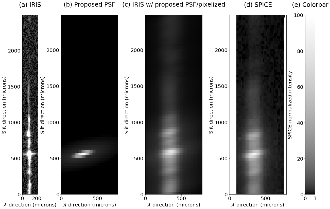
Figure 10 shows the same slit position as what’s shown in Figure 2, with the higher spectral resolution, while Figure 11 shows our final correction with this nominal/ideal SPICE PSF and pixelization. Each figure shows correction of both the SPICE data and the IRIS based ‘synthetic’ SPICE data (IRIS with proposed SPICE PSF and pixelization). All show good removal of the rotation artifacts of the PSF, and the degraded then corrected IRIS data shows a good match to the originals (though not exact, which is to be expected considering the much lower resolution. The high res correction for SPICE (Figure 10) shows the ringing and noise features mentioned, but these are absent when the resolution is reduced back the nominal SPICE values (Figure 11).
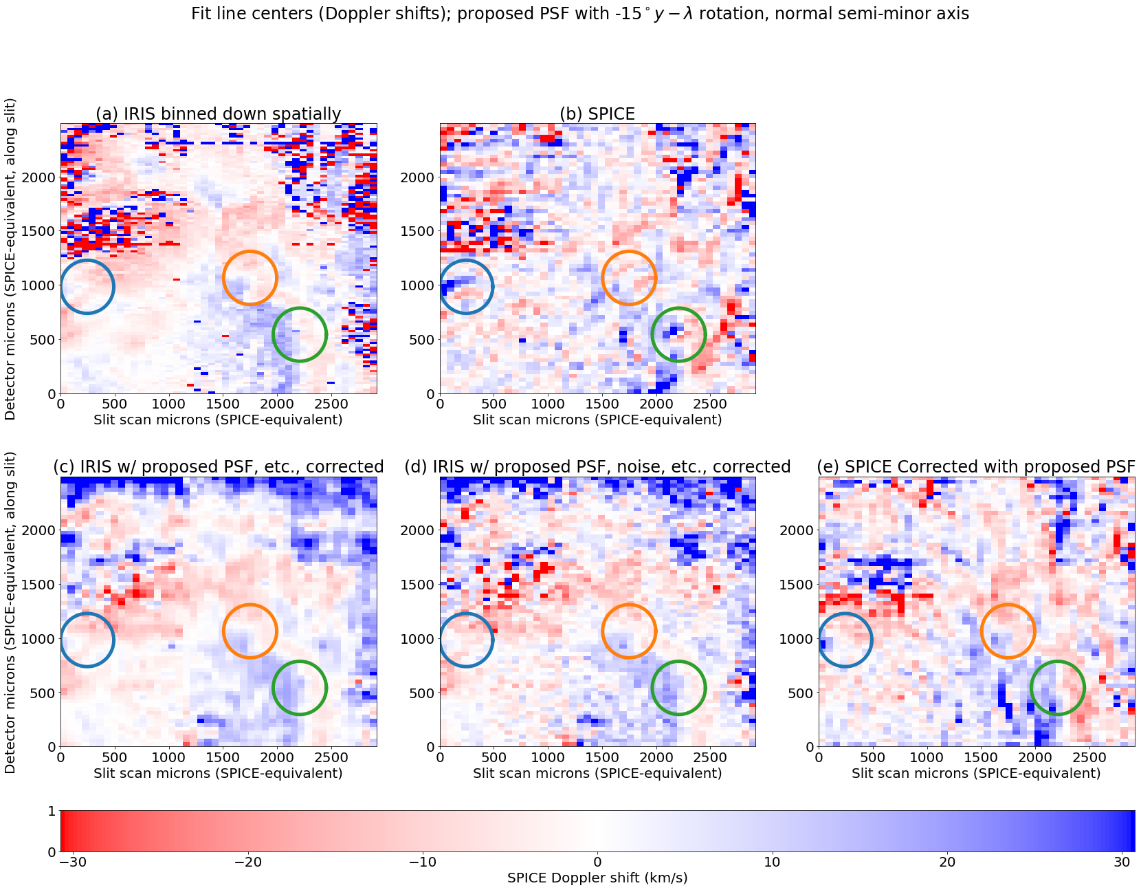
More importantly, the PSF correction does remove the Doppler artifacts, both in the degraded then corrected IRIS data and in the SPICE data. This is shown in Figure 12. This figure has the degraded then corrected IRIS Doppler on left, the degraded IRIS Doppler in center, and the corrected SPICE on right (for original IRIS and SPICE of this data, see Figure 3). The degraded then corrected IRIS is essentially identical to the original (plus binned down) IRIS data, and the SPICE is quite similar to the IRIS. The artifacts previously seen at the circled locations are no longer present. There is some extra coarseness in the SPICE data, due to noise. There are also some artifacts in low signal regions which are likely due to a combination of noise and the interpolation applied to the SPICE L2 data, which we have been using. The interpolation can be mitigated by use of a an intermediate data product (with dark correction and flat fielding but no interpolation), but the low noise limit can’t be – it results in a loss of information that can’t be recovered.
4.1.1 Correction applied to second region
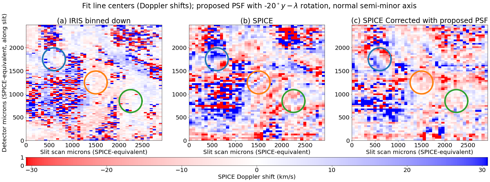
Last, we show correction of a second part of the coordinated IRIS and SPICE observing campaign. This region is more quiet sun, with a couple of isolated bright features (The mean and brightest features are both about a factor of 4 dimmer in this region than in the first one). Removal of artifacts from these features is another good test of the correction of the PSF. A context image for these observations is shown in Figure 13, while Doppler images for the region are shown in Figure 14. The correction removes almost all the artifacts and results in a Doppler image similar to the IRIS data, although somewhat less so than before. A small relatively bright region (circled in blue) in the upper left of the region appears to still have some strong Doppler signals that are not present in IRIS, although they are reduced in magnitude. However, this region has a highly complex spectral structure and varies rapidly spatially and temporally in IRIS, so a close match between SPICE and IRIS isn’t expected here. The corrected ‘synthetic’ SPICE (IRIS degraded with noise added) do not show this artifact, so it would not seem to be an issue with the correction method itself. Nevertheless, it appears as if the ‘corrected’ SPICE data may not be fully corrected in that location. Other differences can be attributed to the lower signal in the region and possibly also to more dissimilarities between the region as seen by IRIS vs. SPICE (the intensities appear more different than in the previous region). We have also had to increase the rotation angle of the PSF from to to best remove the artifacts; the rotation angle does appear to change across the field (we tried a variety of PSF rotation angles for both region, and the ones which best reduced the Doppler artifacts are shown). The correction can account for per-pixel and/or field-wide variation in the PSF, however; it is just a (perhaps not so simple) matter of quantifying that variation.
5 Conclusions
We have shown the presence of Doppler artifacts in the SPICE data and demonstrated that their likely cause is an elongated and rotated effective (i.e., ) PSF. We have further demonstrated a novel method for correcting these artifacts, based on representing the forward transformation as a sparse matrix and then performing a regularized inversion of this matrix with a method based on minimization with norm and positivity constraint.
The correction methods so described appears to work well. It reproduces the IRIS doppler shifts very well when applied to ‘synthetic’ data (IRIS data with SPICE-like PSF and pixelization applied), and quantitatively in most places when applied to real SPICE data. There are some regions where the SNR is too low to correct the PSF and the reconstruction fails for that reason. There are fundamental information limitations to the ability to recover a high-resolution source from a blurred signal, but they do not appear to preclude correction of the Doppler artifacts and restoration of SPICE’s nominal effective PSF. Other issues which presently affect the reconstruction include interpolation of the L2 data and uncertainty in the SPICE PSF, which we hope to rectify using modified data products and further coordinated observations with IRIS and Hinode EIS.
It is also interesting in its applicability to a variety of other problems. The positivity constraint and regularization affords a degree of super-resolution capability, especially when the data being inverted are high-contrast, and so may also be useful for improving the sharpness of high-resolution imagery; unlike many sharpening methods, this method returns a true improved resolution version of its source, maintaining photometry, because its inversion remains consistent with the forward problem and original data. It should also be capable of inverting data from multiple instruments simultaneously, even those with differing resolutions. We may investigate reapplying the method to the DEM problem, for example for doing DEMs using data from AIA and Hinode XRT (Golub et al., 2007) simultaneously. Plowman (2021) applies a similar method to 3D reconstruction of the corona, demonstrating its flexibility.
The corrections shown here were all done on a laptop computer with a 2.6 GHz 6 core Intel Core i7. Although the results shown have been reduced size, we have also carried out correction of full resolution data, on the same laptop. These took hours, considerably less than the average acquisition rate of SPICE data set as a whole. Therefore, the CPU load is easily within the capacity of a central server to reprocess the data, or of individual users to reprocess it on their own. Currently, the codebase has been provided to other members of the SPICE team for beta testing. Once this is finished, the code will be made publicly available. In the meantime, will be provided on request, pending approval of the SPICE team. The code are all written in Python, making use of Numpy (Harris et al., 2020), Astropy (Astropy Collaboration et al., 2013b, 2018b), SciPy (Virtanen et al., 2020b), and optionally SunPy (The SunPy Community et al., 2020b).
Acknowledgements.
This work was supported by NASA under Goddard Space Flight Center subcontract # 80GSFC20C0053 to Southwest Research Institute.References
- Astropy Collaboration et al. (2013a) Astropy Collaboration, Robitaille, T. P., Tollerud, E. J., et al. 2013a, A&A, 558, A33, doi: \hrefhttp://doi.org/10.1051/0004-6361/201322068\nolinkurl10.1051/0004-6361/201322068
- Astropy Collaboration et al. (2013b) —. 2013b, A&A, 558, A33, doi: \hrefhttp://doi.org/10.1051/0004-6361/201322068\nolinkurl10.1051/0004-6361/201322068
- Astropy Collaboration et al. (2018a) Astropy Collaboration, Price-Whelan, A. M., Sipőcz, B. M., et al. 2018a, AJ, 156, 123, doi: \hrefhttp://doi.org/10.3847/1538-3881/aabc4f\nolinkurl10.3847/1538-3881/aabc4f
- Astropy Collaboration et al. (2018b) —. 2018b, AJ, 156, 123, doi: \hrefhttp://doi.org/10.3847/1538-3881/aabc4f\nolinkurl10.3847/1538-3881/aabc4f
- Baker et al. (2005) Baker, A. H., Jessup, E. R., & Manteuffel, T. 2005, SIAM Journal on Matrix Analysis and Applications, 26, 962, doi: \hrefhttp://doi.org/10.1137/S0895479803422014\nolinkurl10.1137/S0895479803422014
- Culhane et al. (2007) Culhane, J. L., Harra, L. K., James, A. M., et al. 2007, Sol. Phys., 243, 19, doi: \hrefhttp://doi.org/10.1007/s01007-007-0293-1\nolinkurl10.1007/s01007-007-0293-1
- De Pontieu et al. (2014) De Pontieu, B., Title, A. M., Lemen, J. R., et al. 2014, Sol. Phys., 289, 2733, doi: \hrefhttp://doi.org/10.1007/s11207-014-0485-y\nolinkurl10.1007/s11207-014-0485-y
- García Marirrodriga et al. (2021) García Marirrodriga, C., Pacros, A., Strandmoe, S., et al. 2021, A&A, 646, A121, doi: \hrefhttp://doi.org/10.1051/0004-6361/202038519\nolinkurl10.1051/0004-6361/202038519
- Golub et al. (2007) Golub, L., Deluca, E., Austin, G., et al. 2007, Sol. Phys., 243, 63, doi: \hrefhttp://doi.org/10.1007/s11207-007-0182-1\nolinkurl10.1007/s11207-007-0182-1
- Harris et al. (2020) Harris, C. R., Millman, K. J., van der Walt, S. J., et al. 2020, Nature, 585, 357, doi: \hrefhttp://doi.org/10.1038/s41586-020-2649-2\nolinkurl10.1038/s41586-020-2649-2
- Lin et al. (2002) Lin, R. P., Dennis, B. R., Hurford, G. J., et al. 2002, Sol. Phys., 210, 3, doi: \hrefhttp://doi.org/10.1023/A:1022428818870\nolinkurl10.1023/A:1022428818870
- Peter et al. (2006) Peter, H., Gudiksen, B. V., & Nordlund, Å. 2006, ApJ, 638, 1086, doi: \hrefhttp://doi.org/10.1086/499117\nolinkurl10.1086/499117
- Plowman (2021) Plowman, J. 2021, arXiv e-prints, arXiv:2103.02028. \hrefhttps://arxiv.org/abs/2103.02028\nolinkurlhttps://arxiv.org/abs/2103.02028
- Plowman & Caspi (2020) Plowman, J., & Caspi, A. 2020, ApJ, 905, 17, doi: \hrefhttp://doi.org/10.3847/1538-4357/abc260\nolinkurl10.3847/1538-4357/abc260
- Poduval et al. (2013) Poduval, B., DeForest, C. E., Schmelz, J. T., & Pathak, S. 2013, ApJ, 765, 144, doi: \hrefhttp://doi.org/10.1088/0004-637X/765/2/144\nolinkurl10.1088/0004-637X/765/2/144
- Press et al. (2002) Press, W., Teukolsky, S., Vetterling, W., & Flannery, B. 2002, Numerical recipes in C: the art of scientific computing (Cambridge University Press)
- Spice Consortium et al. (2020) Spice Consortium, Anderson, M., Appourchaux, T., et al. 2020, A&A, 642, A14, doi: \hrefhttp://doi.org/10.1051/0004-6361/201935574\nolinkurl10.1051/0004-6361/201935574
- The SunPy Community et al. (2020a) The SunPy Community, Barnes, W. T., Bobra, M. G., et al. 2020a, The Astrophysical Journal, 890, 68, doi: \hrefhttp://doi.org/10.3847/1538-4357/ab4f7a\nolinkurl10.3847/1538-4357/ab4f7a
- The SunPy Community et al. (2020b) —. 2020b, The Astrophysical Journal, 890, 68, doi: \hrefhttp://doi.org/10.3847/1538-4357/ab4f7a\nolinkurl10.3847/1538-4357/ab4f7a
- Ugarte-Urra (2016) Ugarte-Urra, I. 2016. https://sohoftp.nascom.nasa.gov/solarsoft/hinode/eis/doc/eis_notes/08_COMA/eis_swnote_08.pdf
- van der Vorst (1992) van der Vorst, H. A. 1992, SIAM Journal on Scientific and Statistical Computing, 13, 631, doi: \hrefhttp://doi.org/10.1137/0913035\nolinkurl10.1137/0913035
- Virtanen et al. (2020a) Virtanen, P., Gommers, R., Oliphant, T. E., et al. 2020a, Nature Methods, 17, 261, doi: \hrefhttp://doi.org/10.1038/s41592-019-0686-2\nolinkurl10.1038/s41592-019-0686-2
- Virtanen et al. (2020b) —. 2020b, Nature Methods, 17, 261, doi: \hrefhttp://doi.org/10.1038/s41592-019-0686-2\nolinkurl10.1038/s41592-019-0686-2
- Young et al. (2012) Young, P. R., O’Dwyer, B., & Mason, H. E. 2012, ApJ, 744, 14, doi: \hrefhttp://doi.org/10.1088/0004-637X/744/1/14\nolinkurl10.1088/0004-637X/744/1/14