Spectroscopic study of four metal-poor carbon stars from the Hamburg/ESO Survey: On confirming the low-mass nature of their companions 111Based on data collected using Mercator/HERMES, SUBARU/HDS
Abstract
Elemental abundances of extrinsic carbon stars provide insight into the poorly understood origin and evolution of elements in the early Galaxy. In this work, we present the results of a detailed spectroscopic analysis of four potential carbon star candidates from the Hamburg/ESO Survey (HES) HE 04571805, HE 09200506, HE 12410337, and HE 13272116. This analysis is based on the high-resolution spectra obtained with Mercator/HERMES (R86,000) and SUBARU/HDS (R50,000). Although the abundances of a few elements, such as, Fe, C, and O are available from medium-resolution spectra, we present the first ever detailed high-resolution spectroscopic analysis for these objects. The object HE 04571805 and HE 12410337 are found to be CEMP-s stars, HE 09200506 a CH star, and HE 13272116 a CEMP-r/s star. The object HE 04571805 is a confirmed binary, whereas the binary status of the other objects is unknown. The locations of program stars on the absolute carbon abundance A(C) vs [Fe/H] diagram point at their binary nature. We have examined various elemental abundance ratios of the program stars and confirmed the low-mass nature of their former AGB companions. We have shown that the i-process models could successfully reproduce the observed abundance pattern in HE 13272116. The parametric model based analysis performed for HE 04571805, HE 09200506, and HE 12410337 based on the FRUITY models confirmed that the surface chemical composition of these three objects are influenced by pollution from low-mass AGB companions.
1 Introduction
The low- and intermediate-mass stars (0.8 - 10 M⊙) are the predominant stellar population of our Galaxy (Karakas & Lattanzio, 2014). These stars are the main sites of various nucloesynthesis and important participants of chemical evolution of the Universe (Travaglio et al., 2001, 2004; Romano et al., 2010; Kobayashi et al., 2011, 2020). As they evolve through different stages of stellar evolution, they enriched the ISM through stellar outflows or winds. The pollution from these low- and intermediate- mass stars account for about 90% of the ISM dust and the massive stars account for the rest (Sloan et al., 2008). Majority of the elements heavier than Fe are produced by these stars through slow- (s-) and rapid- (r-) neutron-capture processes. The origin and evolution of these heavy elements still remains poorly understood. This underscores the need for detailed studies on different classes of stars enhanced in heavy elements, for instance Ba, CH, carbon-enhanced metal-poor (CEMP) stars etc. The last two decades had witnessed a significant increase in the high-resolution spectroscopic studies of these groups of stars.
Ba and CH stars show enhanced abundances of s-process elements. The CEMP-stars are metal-poor counterparts ([Fe/H]1) of CH stars (e.g. Lucatello et al. 2005; Abate et al. 2016). A fraction of them show enrichment of s- and/or r-elements. They are classified into four sub-classes: CEMP-r (enhanced in r-process elements), CEMP-s (enhanced in s-process elements), CEMP-r/s (enhanced in both s- and r-process elements), and CEMP-no (little or no enhancement of heavy elements) (Beers & Christlieb, 2005). The suggested origin for CEMP-r stars is that they were formed from the ISM pre-enriched by events, such as, core-collapse SNe, neutron star mergers, neutron star - black hole mergers (Surman et al., 2008; Arcones & Thielemann, 2013; Rosswog et al., 2014; Drout et al., 2017; Lippuner et al., 2017). The suggested progenitors for the origin of carbon enhancement of CEMP-no stars, that polluted ISM, are faint SNe, spinstar, metal-free massive stars, binary mass-transfer from extremely metal-poor AGB stars (Heger & Woosley, 2010; Nomoto et al., 2013; Chiappini, 2013; Tominaga et al., 2014).
CEMP-s stars are metal-poor analog of CH and Ba stars, and binary mass-transfer from former AGB companion stars have been identified as the source of their observed abundance pattern (e.g. Jorissen et al. 1998; Lucatello et al. 2005; Starkenburg et al. 2014; Jorissen et al. 2016a; Hansen et al. 2016b). However, the exact origin of CEMP-r/s stars is an open question (Jonsell et al., 2006; Masseron et al., 2010; Koch et al., 2019). Studies have shown that almost half of the CEMP-s stars are CEMP-r/s stars (Sneden et al., 2008; Käppeler et al., 2011; Bisterzo et al., 2011). Just like the CEMP-s stars, CEMP-r/s stars are also found to belong to binary systems (Lucatello et al., 2005; Starkenburg et al., 2014; Hansen et al., 2016b). The scenarios proposed to explain the origin of CEMP-r/s stars include: self-pollution of a star formed from r-element enriched ISM, pollution from AGB companion in a binary system formed from r-element enriched ISM, binary system polluted from the massive primary in a tertiary system, secondary star polluted from the primary exploded as Type 1.5 SN or intermediate neutron-capture (i-) process (Jonsell et al. 2006 and references therein, Hampel et al. 2016). The i-process, originally proposed by Cowan & Rose (1977), produces neutron density intermediate between s- and r-process, of the order of 1015-17 cm-3. There are a number of sites proposed to host the i-process, such as Rapidly Accreting White Dwarfs (Denissenkov et al., 2017), super-AGB stars of low-metallicity (Doherty et al., 2015; Jones et al., 2016), metal-poor massive (M 20 M⊙) stars (Banerjee et al., 2018), extremely low-metallicity (z 10-5) low-mass AGB stars (Fujimoto et al., 1990; Hollowell et al., 1990; Lugaro et al., 2009), low-mass (M 2M⊙) very low-metallicity (z 10-4) AGB stars (Fujimoto et al., 2000; Campbell & Lattanzio, 2008; Lau et al., 2009; Cristallo et al., 2009; Campbell et al., 2010; Stancliffe et al., 2011). etc., though exact site(s) is not confirmed yet. Several studies used i-process in low-mass low-metallicity AGB stars to successfully explain the abundances of CEMP-r/s stars (Hampel et al., 2016; Karinkuzhi et al., 2021; Goswami et al., 2021; Shejeelammal et al., 2021; Shejeelammal & Goswami, 2021; Purandardas & Goswami, 2021).
In this work, we have presented the results of a detailed high-resolution spectroscopic analysis of four carbon stars identified from the HES. The structure of the paper is as follows. The stellar sample, source of the spectra and data reduction are discussed in Section 2. Section 3 provides a discussion on radial velocity. Estimation of stellar atmospheric parameters, along with the discussion on stellar mass, is provided in Section 4. In Section 5, we have presented the discussion on abundance determination, followed by a discussion on abundance uncertainties in Section 6. Classification of program stars is presented in Section 7. A detailed discussion on various abundance ratios of the program stars are provided in Section 8. A discussion on the origin of the program stars, along with the parametric model based analysis, is also given in the same section. This section also contains a discussion on individual stars. Conclusions are drawn in Section 9.
2 STELLAR SAMPLE: SELECTION, OBSERVATION/DATA ACQUISITION AND DATA REDUCTION
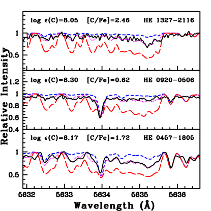
All the four objects, HE 04571805, HE 09200506, HE12410337, and HE 13272116 analysed in this study are selected from the candidate metal-poor stars identified from the Hamburg/ESO survey (HES) (Christlieb, 2003). The stars HE 04571805 and HE 12410337 are listed in the catalog of carbon stars identified from the Hamburg/ESO survey (HES) by Christlieb et al. (2001). The object HE 04571805 is also listed in the list of potential CH star candidates by Goswami (2005). The objects HE 09200506 and HE 13272116 are listed in the catalog of bright metal-poor candidates from the HES by Frebel et al. (2006). The wavelength calibrated, high-resolution (R50,000) spectrum of HE 12410337 is taken from SUBARU/HDS archive (http://jvo.nao.ac.jp/portal/v2/). The wavelength coverage of this spectrum is 4100 - 6850 Å with a wavelength gap between 5440 and 5520 Å. The high-resolution (R86,000) spectra of the objects HE 04571805, HE 09200506, and HE 13272116 were obtained using the High-Efficiency and high-Resolution Mercator Echelle Spectrograph (HERMES) attached to the 1.2m Mercator telescope at the Roque de los Muchachos Observatory in La Palma, Canary Islands, Spain, operated by the Institute of Astronomy of the KU Leuven, Belgium (Raskin et al., 2011). The data were reduced using the HERMES pipeline. The HERMES spectra cover the wavelength range 3770 - 9000 Å. Multiple frames of each object were taken on different nights: 15 frames with exposure of 1800 and 2100 sec for HE 04571805 during the period 2013 - 2016, 10 frames with exposure ranging from 750 - 1800 sec for HE 09100506 during 2018 - 2020, and 3 frames with exposure of 1200 sec for HE 13272116 on 31/01/2019 and 01/02/2019. To maximize the S/N ratio, all these frames were co-added after the Doppler correction. The co-added spectra are then continuum fitted for further analysis, using IRAF222IRAF (Image Reduction and Analysis Facility) is distributed by the National Optical Astronomical Observatories, which is operated by the Association for Universities for Research in Astronomy, Inc., under contract to the National Science Foundation software. Table 1 provides basic information about the program stars, and the sample spectra are shown in Figure 1.
| Star | RA | Dec. | B | V | J | H | K | S/N | ||
|---|---|---|---|---|---|---|---|---|---|---|
| 4200 Å | 5500 Å | 7700 Å | ||||||||
| HE 04571805 | 04 59 43.56 | 18 01 11.99 | 12.372 | 11.014 | 8.937 | 8.421 | 8.186 | 15.82 | 55.48 | 89.05 |
| HE 09200506 | 09 23 05.96 | 05 19 32.75 | 11.80 | 10.95 | 10.317 | 9.971 | 9.900 | 14.00 | 51.88 | 49.89 |
| HE 12410337 | 12 44 27.21 | 03 54 01.20 | 15.84 | 14.30 | 11.869 | 11.234 | 11.026 | 8.35 | 40.16 | – |
| HE 13272116 | 13 30 19.36 | 21 32 03.33 | 12.714 | 11.651 | 9.893 | 9.412 | 9.275 | 13.85 | 29.60 | 68.14 |

3 Radial velocity
The radial velocities of the program stars are estimated from the measured shift in wavelengths of several spectral lines using the Doppler equation. Then, the obtained radial velocity is corrected for heliocentric motion. The average value of these heliocentric motion corrected velocities is taken as the radial velocity of the object. The detailed radial velocity data of the objects analyzed in this study are to be published in a summary paper on orbits of CEMP stars (Jorissen et al., in preparation). The estimated radial velocities, along with the values from the Gaia DR2 (Gaia Collaboration et al., 2018) and RAVE DR4 (Kordopatis et al., 2013), are given in Table 2. The object HE 04571805 is a confirmed binary with an orbital period of 272423 days (Jorissen et al., 2016a). Our radial velocity estimate of this object differ from the Gaia value by 2 km s-1 and from the RAVE value by 9 km s-1. For the object HE 09200506, our estimate shows a difference of 3 km s-1 from the Gaia value. This may indicate that this star is likely a binary. For the other object, HE 13272116, our estimates show a difference of 0.7 km s-1 from the Gaia and RAVE values. The radial velocity estimates for the object HE 12410337 is not available in Gaia and RAVE.
4 STELLAR ATMOSPHERIC PARAMETERS
The stellar atmospheric parameters of the program stars are derived from the measured equivalent widths of the clean Fe I and Fe II lines with excitation potential and equivalent width, respectively, in the range of 0 - 6.0 eV and 10 - 180 mÅ. The radiative transfer code MOOG (Sneden, 1973) is used for our analysis under the assumption of local thermodynamic equilibrium (LTE). The model atmosphere is selected from the Kurucz grid of model atmospheres with no convective overshooting (Castelli & Kurucz 2003, http://kurucz.harvard.edu/grids.html). To select the initial model atmosphere to start with, we have used the photometric temperature estimates calculated from the calibration equations given by Alonso et al. (1999, 2001) and a guess of typical log g value for giants. Using the usual excitation balance and ionization balance method, the final model atmosphere is obtained through an iterative process from the initial one. The detailed procedure is described in our earlier papers Shejeelammal et al. (2020, 2021); Shejeelammal & Goswami (2021). Derived Fe abundances of the program stars are shown in Figure 2, and their derived atmospheric parameters are given in Table 2. The literature values of these atmospheric parameters are also provided in the same table. The comparison of our estimates of stellar atmospheric parameters with the literature values is discussed in Section 8.5.


| Star | Teff | log g | [Fe I/H] | [Fe II/H] | Vr | Vr | Vr | Reference | |
|---|---|---|---|---|---|---|---|---|---|
| (K) | cgs | (km s-1) | (km s-1) | (km s-1) | (km s-1) | ||||
| 100 | 0.2 | 0.2 | (This work) | (Gaia) | RAVE | ||||
| HE 04571805 | 4435 | 0.70 | 1.97 | 1.980.13 | 1.980.12 | +62.830.02 | +60.800.35 | 72.002.2 | 1 |
| 4484 | 0.77 | – | 1.46 | – | – | – | – | 2 | |
| HE 09200506 | 5380 | 2.65 | 0.69 | 0.750.06 | 0.750.01 | +49.600.03 | +52.441.27 | – | 1 |
| – | – | – | 1.01 | – | – | – | – | 3 | |
| 5291 | 2.99 | – | 1.39 | – | – | – | – | 4 | |
| HE 12410337 | 4240 | 1.18 | 2.82 | 2.470.13 | 2.470.09 | +179.692.18 | – | – | 1 |
| HE 13272116 | 4835 | 1.50 | 3.45 | 2.840.07 | 2.840.05 | +176.770.06 | +177.431.46 | 177.41.5 | 1 |
| – | – | – | 2.93 | – | – | – | – | 3 | |
| 4868 | 0.55 | – | 3.48 | – | – | – | – | 4 |
The surface gravity is also calculated from the parallax method using
log (g/g⊙)= log (M/M⊙) + 4log (Teff/Teff⊙) - log (L/L⊙)
The adopted solar values are log g⊙ = 4.44, Teff⊙ = 5770 K, and Mbol⊙ = 4.74 mag.
The masses of the program stars are found from their positions on the H-R diagram (log Teff - log (L/L⊙) diagram)
generated using the evolutionary tracks of Girardi et al. (2000).
This procedure is discussed in detail in Shejeelammal et al. (2020).
For the objects HE 04571805 and HE 13272116, z = 0.0004 ([Fe/H]1.7) tracks were used and
z = 0.004 ([Fe/H]0.7) tracks for HE 09200506. The positions of the program stars on the H-R diagram are
shown in Figure 3.
We could find only an upper limit to the
mass of the star HE 04571805. We could not estimate the mass of the star HE 12410337
since its parallax value is not available. The estimated mass and log g values of the program stars
are given in Table 3. For the star HE 09200506, the spectroscopic log g
is 0.8 dex lower than that estimated from the parallax method.
In some carbon stars, such an inconsistency between the spectroscopic atmospheric parameters and
those derived from the evolutionary tracks could arise as their evolutionary tracks shift
towards lower temperatures (Marigo, 2002; Jorissen
et al., 2016b).
The spectroscopic log g values have been used for our analysis.


| Star name | Parallax | Mbol | log(L/L⊙) | Mass(M⊙) | log g | log g (spectroscopic) |
|---|---|---|---|---|---|---|
| (mas) | (cgs) | (cgs) | ||||
| HE 04571805 | 0.4670.0309 | 1.3410.14 | 2.430.05 | 0.60 | – | 0.70 |
| HE 09200506 | 2.37640.0653 | 2.4880.06 | 0.900.02 | 1.300.005 | 3.500.03 | 2.65 |
| HE 13272116 | 0.34280.0358 | 1.1300.228 | 2.350.09 | 0.700.10 | 1.630.03 | 1.50 |
5 Abundance determination
The elemental abundances were estimated from two methods: (i) using the equivalent widths of the spectral lines and (ii) by comparison of observed spectra and synthetic spectra generated with MOOG (spectral synthesis calculation), using Kurucz model atmospheres (http://kurucz.harvard.edu/grids.html). The spectral synthesis calculation is performed to derive the abundances of elements with hyper-fine splitting (HFS) as well as for molecular bands. The hyper-fine components of each atomic line, whenever available, are considered for the abundance estimation. In the case of abundance determination using the equivalent width method, the spectral line identification is performed by comparing the stellar spectra with the Doppler corrected spectrum of Arcturus. The line parameters are taken from linemake 333linemake contains laboratory atomic data (transition probabilities, hyperfine and isotopic substructures) published by the Wisconsin Atomic Physics and the Old Dominion Molecular Physics groups. These lists and accompanying line list assembly software have been developed by C. Sneden and are curated by V. Placco at https://github.com/vmplacco/linemake. atomic and molecular line database (Placco et al., 2021).
Although the abundance estimation is performed under the assumption of LTE, we have applied the non-LTE (NLTE) corrections whenever available. The solar abundance values are adopted from Asplund et al. (2009). The details of the abundances of each elements and the details of NLTE corrections as well as HFS are discussed in this section. The estimated elemental abundances in the program stars are given in Tables 4 and 5. The atomic lines used to derive the abundances of each elemental species are given in Tables 9 - 11.
| HE 04571805 | HE 09200506 | |||||||||
| Z | solar log | log | [X/H] | [X/Fe] | N | log | [X/H] | [X/Fe] | N | |
| C† (C2 band 5165 Å) | 6 | 8.43 | 8.32 | 0.11 | 1.87 | – | 8.20 | 0.23 | 0.52 | – |
| C† (C2 band 5635 Å) | 6 | 8.43 | 8.17 | 0.26 | 1.72 | – | 8.30 | 0.13 | 0.62 | – |
| 12C/13C† | – | – | – | – | 234 | – | – | – | – | – |
| N† | 7 | 7.83 | 7.520.07 | 0.31 | 1.67 | 3 | 7.530.20 | 0.30 | 0.45 | 3 |
| O† | 8 | 8.69 | – | – | – | – | 7.80 | 0.89 | 0.14 | 1 |
| Na I | 11 | 6.24 | 6.460.06 | 0.22 | 2.2 | 3 | 5.940.09 | 0.30 | 0.45 | 3 |
| Mg I | 12 | 7.6 | 6.940.14 | 0.66 | 1.32 | 2 | 7.500.03 | 0.10 | 0.65 | 3 |
| Si I | 14 | 7.51 | 5.980.17 | 1.53 | 0.45 | 2 | 7.140.17 | 0.37 | 0.38 | 2 |
| Ca I | 20 | 6.34 | 5.210.12 | 1.13 | 0.85 | 7 | 5.980.11 | 0.36 | 0.39 | 16 |
| Sc II† | 21 | 3.15 | 1.85 | 1.30 | 0.68 | 1 | 2.14 | 1.09 | 0.26 | 2 |
| Ti I | 22 | 4.95 | 3.830.17 | 1.12 | 0.86 | 6 | 4.400.08 | 0.55 | 0.2 | 8 |
| Ti II | 22 | 4.95 | 3.400.14 | 1.55 | 0.43 | 5 | 4.340.08 | 0.61 | 0.14 | 8 |
| V I† | 23 | 3.93 | 2.73 | 1.20 | 0.78 | 2 | 2.87 | 1.06 | 0.31 | 1 |
| Cr I | 24 | 5.64 | 4.720.10 | 0.92 | 1.06 | 4 | 5.360.09 | 0.28 | 0.47 | 10 |
| Cr II | 24 | 5.64 | 4.580.04 | 1.06 | 0.92 | 2 | 5.370.07 | 0.27 | 0.48 | 3 |
| Mn I† | 25 | 5.43 | 4.43 | 1.00 | 0.98 | 2 | 4.440.01 | 0.99 | 0.24 | 2 |
| Fe I | 26 | 7.5 | 5.520.13 | 1.98 | – | 11 | 6.750.06 | 0.75 | – | 17 |
| Fe II | 26 | 7.5 | 5.520.12 | 1.98 | – | 4 | 6.750.01 | 0.75 | – | 3 |
| Co I† | 27 | 4.99 | 3.58 | 1.41 | 0.57 | 1 | 4.19 | 0.80 | 0.05 | 1 |
| Ni I | 28 | 6.22 | 5.300.08 | 0.92 | 1.06 | 7 | 5.830.10 | 0.39 | 0.36 | 10 |
| Cu I† | 29 | 4.19 | 2.21 | 1.98 | 0 | 1 | 3.19 | 1.00 | 0.25 | 1 |
| Zn I | 30 | 4.56 | 3.10 | 1.50 | 0.48 | 1 | 4.340.12 | 0.22 | 0.53 | 2 |
| Rb I† | 37 | 2.52 | 1.95 | 0.57 | 1.41 | 1 | 1.70 | 0.82 | 0.07 | 1 |
| Sr INLTE† | 38 | 2.87 | 2.54 | 0.33 | 1.65 | 1 | 3.57 | 0.7 | 1.45 | 1 |
| Y I† | 39 | 2.21 | 3.01 | 0.8 | 2.78 | 1 | 2.32 | 0.11 | 0.86 | 1 |
| Y II | 39 | 2.21 | 2.180.20 | 0.03 | 1.95 | 4 | 2.670.11 | 0.46 | 1.21 | 6 |
| Zr I† | 40 | 2.58 | 3.03 | 0.45 | 2.43 | 1 | 3.05 | 0.47 | 1.22 | 1 |
| Zr II† | 40 | 2.58 | 2.63 | 0.05 | 2.03 | 1 | 2.38 | 0.20 | 0.55 | 1 |
| Ba IILTE† | 56 | 2.18 | – | – | – | – | 2.83 | 0.65 | 1.4 | 1 |
| Ba IINLTE† | 56 | 2.18 | 2.73 | 0.55 | 2.53 | 1 | 2.83 | 0.65 | 1.4 | 1 |
| La II† | 57 | 1.1 | 1.390.02 | 0.29 | 2.27 | 3 | 1.60 | 0.5 | 1.25 | 2 |
| Ce II | 58 | 1.58 | 1.950.15 | 0.37 | 2.35 | 6 | 1.990.14 | 0.41 | 1.16 | 6 |
| Pr II | 59 | 0.72 | 1.300.11 | 0.58 | 2.56 | 6 | 1.150.03 | 0.43 | 1.18 | 2 |
| Nd II | 60 | 1.42 | 1.810.11 | 0.39 | 2.37 | 9 | 1.740.14 | 0.32 | 1.07 | 4 |
| Sm II | 62 | 2.41 | 1.390.11 | 0.43 | 2.41 | 7 | 1.570.18 | 0.61 | 1.36 | 4 |
| Eu IILTE† | 63 | 0.52 | 0.20 | 0.72 | 1.26 | 1 | 0.39 | 0.91 | 0.16 | 1 |
| Eu IINLTE† | 63 | 0.52 | – | – | – | – | 0.43 | 0.95 | 0.20 | 1 |
Asplund et al. (2009). † indicates that the abundances are derived from spectral synthesis method. N is the number of lines used to derive the abundance. NLTE refers to the abundance derived from the lines affected by NLTE, after the corrections being applied.
| HE 12410337 | HE 13272116 | |||||||||
|---|---|---|---|---|---|---|---|---|---|---|
| Z | solar log | log | [X/H] | [X/Fe] | N | log | [X/H] | [X/Fe] | N | |
| C† (C2 band 5165 Å) | 6 | 8.43 | – | – | – | – | 8.05 | 0.38 | 2.46 | – |
| C† (C2 band 5635 Å) | 6 | 8.43 | 8.53 | 0.10 | 2.57 | – | 8.05 | 0.38 | 2.46 | – |
| 12C/13C† | – | – | – | – | – | – | – | – | 73 | – |
| N† | 7 | 7.83 | 6.38 | 1.45 | 1.02 | – | 7.500.10 | 0.33 | 2.51 | 3 |
| Na I | 11 | 6.24 | 5.350.18 | 0.89 | 1.58 | 2 | 4.28 | 1.96 | 0.88 | 1 |
| Mg I | 12 | 7.6 | 5.170.13 | 2.43 | 0.04 | 2 | 5.22 | 2.38 | 0.46 | 1 |
| Si I | 14 | 7.51 | 5.820.10 | 1.69 | 0.78 | 2 | 5.45 | 2.06 | 0.78 | 1 |
| Ca I | 20 | 6.34 | 4.150.15 | 2.19 | 0.28 | 6 | 4.130.06 | 2.21 | 0.63 | 5 |
| Sc II† | 21 | 3.15 | 1.000.13 | 2.15 | 0.32 | 2 | 0.030.01 | 3.12 | 0.27 | 2 |
| Ti I | 22 | 4.95 | 2.770.12 | 2.18 | 0.29 | 3 | 2.770.02 | 2.18 | 0.66 | 2 |
| Ti II | 22 | 4.95 | 2.530.19 | 2.42 | 0.05 | 4 | 2.590.08 | 2.36 | 0.48 | 4 |
| Cr I | 24 | 5.64 | – | – | – | – | 3.030.01 | 2.61 | 0.23 | 2 |
| Cr II | 24 | 5.64 | 3.550.03 | 2.09 | 0.38 | 2 | – | – | – | – |
| Mn I† | 25 | 5.43 | 3.55 | 1.88 | 0.59 | 1 | 3.610.03 | 1.81 | 1.03 | 2 |
| Fe I | 26 | 7.5 | 5.030.13 | 2.47 | - | 16 | 4.660.07 | 2.84 | - | 11 |
| Fe II | 26 | 7.5 | 5.030.09 | 2.47 | - | 3 | 4.660.04 | 2.84 | - | 2 |
| Co I | 27 | 4.99 | – | – | – | – | 1.810.07 | 3.18 | 0.34 | 2 |
| Ni I | 28 | 6.22 | 3.640.15 | 2.58 | 0.11 | 4 | 4.690.06 | 1.53 | 1.31 | 3 |
| Zn I | 30 | 4.56 | 1.81 | 2.75 | 0.28 | 1 | 2.16 | 2.40 | 0.44 | 1 |
| Sr INLTE† | 38 | 2.87 | 1.54 | 1.33 | 1.14 | 1 | – | – | – | – |
| Y II | 39 | 2.21 | 0.860.11 | 1.35 | 1.12 | 5 | 0.060.02 | 2.15 | 0.69 | 2 |
| Zr I† | 40 | 2.58 | 1.44 | 1.14 | 1.33 | 1 | 1.81 | 0.77 | 2.07 | 1 |
| Zr II | 40 | 2.58 | 1.540.04 | 1.04 | 1.43 | 4 | 0.89† | 1.69 | 1.15 | 1 |
| Ba IINLTE† | 56 | 2.18 | 0.75 | 1.43 | 1.04 | 1 | 1.08 | 1.10 | 1.74 | 1 |
| La II† | 57 | 1.1 | 0.35 | 1.45 | 1.02 | 1 | 0 | 1.10 | 1.74 | 1 |
| Ce II | 58 | 1.58 | 0.270.19 | 1.31 | 1.16 | 3 | 0.490.10 | 1.09 | 1.75 | 5 |
| Pr II | 59 | 0.72 | 0.430.12 | 1.15 | 1.32 | 3 | 0.23 | 0.95 | 1.89 | 1 |
| Nd II | 60 | 1.42 | 0.030.12 | 1.45 | 1.02 | 4 | 0.360.08 | 1.06 | 1.78 | 8 |
| Sm II | 62 | 2.41 | 0.520.01 | 1.48 | 0.99 | 2 | 0.070.15 | 1.03 | 1.81 | 4 |
| Eu IILTE† | 63 | 0.52 | 1.430.15 | 1.95 | 0.52 | 2 | 1.16 | 1.68 | 1.16 | 1 |
Asplund et al. (2009). † indicates that the abundances are derived from spectral synthesis method. N is the number of lines used to derive the abundance. NLTE refers to the abundance derived from the lines affected by NLTE, after the corrections being applied.
5.1 Light elements: C, N, O, 12C/13C, Na, -, and Fe-peak elements
The oxygen abundance could be derived only in HE 09200506 where we have used the spectral synthesis calculation of [O I] line at 6300.304 Å. Oxygen is found to be slightly under abundant in this star with a value [O/Fe]0.14. We could not detect good [O I] 6300.304 Å line in other stars. The [O I] line at 6363.776 Å and oxygen triplet at 7770 Å were not usable for abundance determination in any of the program stars.
We could determine the carbon abundance in all the four program stars. The carbon abundance is derived from the spectral synthesis calculation of C2 bands around 5165 and 5635 Å except for HE 12410337 where the C2 5165 Å band is noisy. The carbon abundances estimated from these two bands are consistent within 0.15 dex, and the final carbon abundance is taken to be the average of these two abundance values. While the star HE 09200506 shows a moderate enhancement of carbon with [C/Fe]0.57, the other three stars are enhanced in carbon with [C/Fe]1.70. The spectral synthesis fits of the two carbon bands in the program stars are shown in Figure 4.
We could estimate nitrogen in all the program stars. In HE 12410337, the nitrogen abundance is estimated from the spectrum synthesis of 12CN band at 4215 Å. In the other three program stars, nitrogen abundance is derived from the spectral synthesis calculation of 12CN lines around 8000 Å. Among the program stars, the object HE 13272116 shows the highest enhancement of nitrogen with [N/Fe]2.51.
The carbon isotopic ratio, 12C/13C, is derived using the spectral synthesis calculation of 12CN and 13CN lines around 8000 Å. We could not estimate the value of 12C/13C ratio in HE 09200506 as the 13CN lines were not good, and in HE 12410337 as this region is not present in its spectrum. The values obtained for this ratio in the stars HE 04571805 and HE 13272116 are 234 and 73 respectively.

The abundances of elements Na, Mg, Si, Ca, Ti, Cr, Ni, and Zn are estimated from the measured equivalent widths of spectral lines listed in Table 10. We could estimate the abundances of all these elements in all the program stars. The object HE 04571805 shows the largest enhancement of Na with [Na/Fe]2.20. While HE 12410337 and HE 13272116 show an enhancement of [Na/Fe]1.58 and 0.88 respectively, Na is moderately enhanced in HE 09200506 with [Na/Fe]0.45. In very metal-poor stars, Na suffers large uncertainties due to NLTE corrections or 3D hydrodynamical model atmospheres (Bisterzo et al., 2011; Andrievsky et al., 2007). The NLTE effect may reduce the Na abundance by up to 0.7 dex (Andrievsky et al., 2007). However, the Na I 5682.633, 5688.205, 6154.226 and 6160.747 Å lines have negligible NLTE effect (Takeda et al., 2003; Lind et al., 2011). We have used these weak lines to derive the Na abundance. The Mg abundance is derived mainly from Mg I 4702.991, 5528.405, 5711.088 Å lines. The object HE 04571805 is enhanced in Mg as well with [Mg/Fe]1.32. The object HE 12410337 shows a near-solar value, whereas the other two objects show moderate enhancement of Mg.
We have used the spectral synthesis calculation to derive the abundances of elements Sc, V, Mn, Co and Cu by incorporating their hyper-fine components, whenever available. The Sc II 6245.637 Å line is used to derive Sc abundance in HE 04571805, Sc II 6245.637, 6604.601 Å lines were used HE 09200506. The Sc II lines at 4320.732, 4415.556 Å were used in HE 12410337. In the case of HE 13272116, Sc II 4374.457, 5031.021 Å lines were used. In HE 09200506 and HE 13272116, scandium is slightly under abundant with [Sc/Fe]0.25, while it is moderately enhanced in other two stars. Vanadium abundance is derived from the spectral synthesis calculation of V I 4864.731, 5727.048 Å lines. We could not estimate vanadium abundance in HE 12410337 and HE 13272116 as there is no clean lines available. The objects HE 04571805 and HE 09200506 show [V/Fe] value 0.78 and 0.31 respectively. Manganese abundance is derived from the spectral synthesis calculation of Mn I 6013.513, 6021.89 Å lines in the stars HE 04571805 and HE 09200506. The Mn I 5516.743 Å line is used in HE 12410337, and Mn I lines at 4451.586 and 4470.140 Å were used in the case of HE 13272116. We have used the Co I 4118.770, 4121.320, 5342.695, 5483.344 Å lines to estimate the cobalt abundance. We could not estimate the cobalt abundance in HE 12410337 as no good lines were found in the spectrum. The cobalt abundances, [Co/Fe], in the program stars are in the range 0.34 - +0.57. Copper abundance is derived using the line Cu I 5105.537 Å.
5.2 Heavy elements
5.2.1 The light s-process elements: Rb, Sr, Y, Zr
The rubidium abundance is derived from the spectral synthesis calculation of Rb I resonance line at 7800.259 Å. The HFS components of this line are taken from (Lambert & Luck, 1976). The other Rb I line at 7947.597 Å was not usable for abundance determination in any of the program stars. We could not derive the Rb abundance in HE 12410337 as this region is absent in the spectrum, and in HE 13272116 as we could not detect any good lines due to Rb. While Rb is found to be enhanced in HE 04571805 with [Rb/Fe]1.41, it shows near-solar value in HE 09200506.
We have estimated the Sr abundance using the spectral synthesis calculation of Sr I 4607.327 Å line. This line is known to be affected by NLTE effect, and the appropriate NLTE corrections are adopted from Bergemann et al. (2012). The Sr abundance could be determined in all the program stars except HE 13272116, and it is found to be enhanced with [Sr/Fe]1.10. The NLTE corrections to the abundances of Sr for HE 04571805 and HE 12410337 are +0.47, and for HE 09200506 is +0.17.
Yttrium abundance is derived from the spectral synthesis calculation of Y I 6435.004 Å line and from the measured equivalent widths of several Y II lines listed in Table 10. While we could estimate Y II abundance in all the program stars, Y I abundance could not be determined in HE 12410337 and HE 13272116 as we could not detect any good Y I lines. The Y II abundance, [Y II/Fe], ranges from 0.69 to 1.95, whereas Y I abundances, [Y I/Fe], are 2.78 and 0.86 respectively in HE 04571805 and HE 09200506.
We have estimated the Zr abundance from the spectral synthesis calculation of Zr I 6134.585 Å line in all the stars. The Zr II abundance is derived from the measured equivalent widths of several Zr II lines in HE 12410337 and spectral synthesis of Zr II 5112.297 Å line in other three program stars. While Zr I abundances, [Zr I/Fe], ranges from 1.22 to 2.43, Zr II abundances, [Zr II/Fe], ranges from 0.55 to 2.03.
5.2.2 The heavy s-process elements: Ba, La, Ce, Pr, Nd
In all program stars, abundance of Ba is derived from the spectral synthesis calculation of Ba II 5853.668 Å line by incorporating the hyperfine components. The NLTE corrections to the abundances derived from this line are adopted from Andrievsky et al. (2009). The NLTE correction for HE 12410337 is +0.05, HE 13272116 is +0.28, and 0.00 for other two stars. We could also use Ba II 6496.897 Å in the object HE 09200506. In other stars, this line is not usable. The Ba II 4934.076, 6141.713 Å lines were either strong (equivalent width240 mÅ) or not good to be used for abundance determination in all the objects. Ba is found to be enhanced in all the program stars with [Ba/Fe]1.0. The spectral synthesis fits for Ba II 5853.668 and 6496.897 Å lines for the star HE 09200506 are shown in Figure 5.

The La abundance is derived from the spectral synthesis calculation of La II lines at 4748.726, 4921.776, 5259.379, and 5303.528 Å, whenever possible, by incorporating the HFS components. The HFS components of La II 4748.726, 5259.379 Å lines were not available. All the program stars show enhancement of La with [La/Fe]1, HE 04571805 being the most enriched in La with a value [La/Fe]2.27.
The abundances of Ce, Pr, and Nd are derived using the equivalent widths measured from several lines of the singly ionized species of these elements. The atomic lines used for the abundance determination of these elements are given in Table 10. All the program stars are found to show enhancement of [X/Fe]1 for all these elements.
We have also calculated the [ls/Fe], [hs/Fe], [hs/ls] ratios of the program stars. Here, ls stands for light s-process elements: Sr, Y and Zr, and hs stands for heavy s-process elements: Ba, La, Ce and Nd. We have also calculated the [s/Fe] ratio, a measure of total s-process content of a star, for all the program stars. Here s refers to the s-process elements Sr, Y, Zr, Ba, La, Ce, and Nd. The [hs/Fe] is calculated as ([Ba/Fe] + [La/Fe] + [Ce/Fe] + [Nd/Fe])/4, [ls/Fe] as ([Sr/Fe] + [Y/Fe] + [Zr/Fe])/3 and [s/Fe] as ([Sr/Fe] + [Y/Fe] + [Zr/Fe] + [Ba/Fe] + [La/Fe] + [Ce/Fe] + [Nd/Fe])/7. Values of these ratios are given in Table 6. As seen from the table, all our stars have high s-process content with [s/Fe]. We could estimate the [Rb/Zr] ratio, an indicator of neutron density at s-process site and mass of companion AGB star, for two objects. Estimated values of this ratio are also provided in Table 6. These ratios will be discussed in detail later in this paper.
| Star name | [Fe/H] | [ls/Fe] | [hs/Fe] | [s/Fe] | [hs/ls] | [Rb/Zr] |
|---|---|---|---|---|---|---|
| HE 04571805 | 1.98 | 1.88 | 2.38 | 2.16 | 0.50 | 1.02 |
| HE 09200506 | 0.75 | 1.29 | 1.22 | 1.15 | 0.07 | 1.29 |
| HE 12410337 | 2.47 | 1.20 | 1.06 | 1.31 | 0.14 | – |
| HE 13272116 | 2.84 | 0.92 | 1.75 | 1.48 | 0.83 | – |
5.2.3 The r-process elements: Sm, Eu
We have used the measured equivalent widths of several Sm II lines listed in Table 10 to derive the abundance of Sm. All the stars show enhanced abundance of Sm with [Sm/Fe]0.99. The abundance of Eu is derived from the spectral synthesis calculation of Eu II 6645.064 Å line in all the four program stars. We could also use Eu II line at 4129.725 Å in HE 09200506, and Eu II 6437.640 Å line in HE 12410337. The Eu II 4129.725 Å line is affected by NLTE, and the correction to the abundance derived from this line (+0.16) is adopted from Mashonkina et al. (2008). While Eu is mildly under abundant in HE 09200506 with [Eu/Fe]0.20, it is moderately enhanced in HE 12410337 with [Eu/Fe]0.52. The other two stars HE 04571805 and HE 13272116 are enhanced in Eu with [Eu/Fe] value around 1.20.
6 ABUNDANCE UNCERTAINTIES
The uncertainty in the abundances of each element is calculated following the procedure in Shejeelammal et al. (2020) using;
= + + + +
Here, is the total uncertainty in the absolute
abundance of the particular element. The is the random
error which is calculated from the standard deviation () of
the abundances derived from N lines of the particular element using
= .
The , , and
are the typical uncertainties in the stellar atmospheric parameters, which are
100 K, 0.2 dex,
0.2 km s-1 and 0.1 dex.
The abundance uncertainty in the abundance ratio of an element, X, is calculated
from;
= + .
We made the calculation simple by assuming that the parameters are independent. Hence, the uncertainties calculated here are taken to be the upper limits. The changes in the abundances of each element with the variation in different atmospheric parameters are given in Table 7. We have evaluated the differential abundances in the specific case of the star HE 09200506.
| Element | Teff | log g | [Fe/H] | ||
|---|---|---|---|---|---|
| (100 K) | (0.2 dex) | (0.2 km s-1) | (0.1 dex) | ||
| C | 0.07 | 0.10 | 0.10 | 0.10 | 0.23 |
| N | 0.13 | 0.03 | 0.00 | 0.02 | 0.19 |
| O | 0.00 | 0.04 | 0.02 | 0.00 | 0.14 |
| Na I | 0.04 | 0.01 | 0.02 | 0.01 | 0.15 |
| Mg I | 0.07 | 0.06 | 0.03 | 0.01 | 0.16 |
| Si I | 0.04 | 0.00 | 0.02 | 0.00 | 0.18 |
| Ca I | 0.08 | 0.04 | 0.07 | 0.00 | 0.17 |
| Sc II | 0.01 | 0.08 | 0.04 | 0.02 | 0.19 |
| Ti I | 0.11 | 0.01 | 0.07 | 0.01 | 0.19 |
| Ti II | 0.01 | 0.06 | 0.10 | 0.02 | 0.18 |
| V I | 0.13 | 0.04 | 0.13 | 0.00 | 0.23 |
| Cr I | 0.10 | 0.03 | 0.09 | 0.01 | 0.19 |
| Cr II | 0.04 | 0.08 | 0.06 | 0.02 | 0.20 |
| Mn I | 0.08 | 0.01 | 0.08 | 0.01 | 0.17 |
| Fe I | 0.09 | 0.00 | 0.09 | 0.01 | – |
| Fe II | 0.05 | 0.08 | 0.13 | 0.03 | – |
| Co I | 0.11 | 0.00 | 0.03 | 0.01 | 0.17 |
| Ni I | 0.07 | 0.02 | 0.07 | 0.01 | 0.17 |
| Cu I | 0.11 | 0.02 | 0.16 | 0.01 | 0.23 |
| Zn I | 0.01 | 0.02 | 0.09 | 0.00 | 0.18 |
| Rb I | 0.10 | 0.00 | 0.03 | 0.00 | 0.17 |
| Sr I | 0.11 | 0.04 | 0.18 | 0.00 | 0.25 |
| Y I | 0.16 | 0.00 | 0.01 | 0.01 | 0.21 |
| Y II | 0.01 | 0.05 | 0.14 | 0.02 | 0.23 |
| Zr I | 0.12 | 0.00 | 0.05 | 0.02 | 0.18 |
| Zr II | 0.01 | 0.06 | 0.17 | 0.01 | 0.24 |
| Ba II | 0.05 | 0.02 | 0.10 | 0.04 | 0.20 |
| La II | 0.04 | 0.03 | 0.20 | 0.02 | 0.26 |
| Ce II | 0.02 | 0.08 | 0.14 | 0.02 | 0.24 |
| Pr II | 0.03 | 0.08 | 0.03 | 0.02 | 0.19 |
| Nd II | 0.03 | 0.07 | 0.13 | 0.02 | 0.23 |
| Sm II | 0.03 | 0.07 | 0.11 | 0.02 | 0.23 |
| Eu II | 0.04 | 0.07 | 0.26 | 0.03 | 0.27 |
7 Classification of the program stars
Among our stellar sample, HE 04571805, HE 12410337, and HE 13272116 are found to be metal-poor objects with [Fe/H]1, whereas HE 09200506 is moderately metal-poor with [Fe/H]0.75. CEMP stars are traditionally being classified as the metal-poor stars with [C/Fe]1 (Beers & Christlieb, 2005). This classification criteria is being refined and many authors use different threshold values for [C/Fe] to define CEMP stars. However, the carbon abundance is related to the evolutionary stages of the stars. In the case of evolved metal-poor giant stars, the surface carbon abundance could be altered through CNO cycle as a result of internal mixing. This internal mixing processes are First Dredge-Up (FDU) on the giant branch and some extra mixing at the tip of RGB (Charbonnel, 1995; Charbonnel et al., 1998; Gratton et al., 2000; Shetrone, 2003; Jacobson et al., 2005; Spite et al., 2005, 2006; Aoki et al., 2007; Placco et al., 2014). Hence, using a fixed [C/Fe] value to define CEMP stars without considering the evolutionary effects would be incomplete. Here, we have adopted the empirical definition of Aoki et al. (2007) to distinguish the CEMP stars of our sample. This definition is shown schematically in Figure 6. As seen from this figure, while HE 04571805 and HE 13272116 are CEMP stars, HE 09200506 is a non-CEMP star. From the C/O value (1) of HE 09200506, we found that it is a CH star. We could not locate the star HE 12410337 in this diagram as we could not find its luminosity due to the unavailability of parallax. However, the higher [C/Fe] value (2.57) of this star place it in the CEMP category.

We have adopted the classification scheme given by Goswami
et al. (2021) to
sub-classify our CEMP stars. This classification scheme considers
[Ba/Eu] and [La/Eu] ratios of the stars, which is given as;
-CEMP-s; [Ba/Fe]1
(i) [Eu/Fe]1, [Ba/Eu]0 and/or [La/Eu]0.5
(ii) [Eu/Fe]1, [Ba/Eu]1 and/or [La/Eu]0.7
-CEMP-r/s; [Ba/Fe]1, [Eu/Fe]1
(iii) 0[Ba/Eu]1 and/or 0[La/Eu]0.7
Figure 7 schematically represents this classification. The values of [C/Fe], [Ba/Eu], [La/Eu] ratios observed in the program stars are given in Table 8. In Figure 7, the above conditions (i) and (ii) of CEMP-s stars are marked as region (i) and (ii) respectively, and CEMP-r/s condition is marked as region (iii). From this figure and Table 8, the object HE 04571805 and HE 12410337 are found to be CEMP-s stars (region (ii) and (i) respectively) and the object HE 13272116 is found to be a CEMP-r/s star (region (iii)).
| Star name | [Fe/H] | [C/Fe] | [Ba/Fe] | [La/Fe] | [Eu/Fe] | [Ba/Eu] | [La/Eu] |
|---|---|---|---|---|---|---|---|
| HE 04571805 | 1.98 | 1.80 | 2.53 | 2.27 | 1.26 | 1.43 | 1.01 |
| HE 09200506 | 0.75 | 0.57 | 1.40 | 1.25 | 0.20 | 1.60 | 1.45 |
| HE 12410337 | 2.47 | 2.57 | 1.04 | 1.02 | 0.52 | 0.52 | 0.50 |
| HE 13272116 | 2.84 | 2.46 | 1.74 | 1.74 | 1.16 | 0.58 | 0.58 |


8 Discussion
8.1 Comparison of the observed abundance
We have compared the observed abundances of light as well as heavy elements in our program stars with those in CH, Ba, CEMP, and normal stars from literature, and are shown in Figures 8 and 9. All the s-process elements in the program stars show enhanced abundances compared to the normal stars. All the light elements except Na, Mg, V, Cr, Mn, and Ni show abundances similar to that seen in normal stars of the Galaxy. In HE 04571805 the elements Na, Mg, V, Cr, Mn and Ni are enhanced when compared to normal giants. Similarly, Mn and Ni are enhanced in HE 13272116. Similar enhancements of Na, Mg and/or Fe-peak elements in CEMP stars were reported in literature (Aoki et al., 2006; Frebel et al., 2008; Bessell et al., 2015; Shejeelammal & Goswami, 2021; Goswami et al., 2021; Purandardas & Goswami, 2021). Several sources such as faint SNe, spinstars, AGB mass transfer combined with metal accretion from the ISM have used to explain their abundance patterns (Aoki et al., 2006; Frebel et al., 2008; Bessell et al., 2015). According to Choplin et al. (2017), multiple sources may contribute to the formation of CEMP stars. This may be a possible reason for the observed enhancement of these elements. It is possible that the natal clouds of the CEMP stars might get polluted from multiple faint SNe events in the past. A study by Hartwig et al. (2018) has presented a number of reliable tracers to identify whether the natal clouds of CEMP stars are mono- or multi-enriched. According to them, the elemental ratios [Mg/C]1, [Sc/Mn]0.5, [C/Cr]0.5 or [Ca/Fe]2 indicates mono-enrichment. We found [Ca/Fe]2 in our program stars HE 04571805 and HE 13272116, which may indicate that these stars were formed from the gas cloud enriched by multiple SNe events. This may also be a possible reason for the enhanced abundances of the above mentioned elements in these stars. Enhanced Na and/or Mg abundances are observed in a few CEMP-s and CEMP-r/s stars (Bisterzo et al., 2011; Allen et al., 2012; Karinkuzhi et al., 2021; Goswami et al., 2021; Shejeelammal & Goswami, 2021). We have discussed the Na and Mg abundances in detail in section 8.3.2.


8.2 Carbon abundance and possible origin of program stars
Studies have shown that the absolute carbon abundances, A(C), of CEMP stars show bimodality, that is they tend to plateau around two distinct A(C) values in the A(C) - [Fe/H] diagram (Spite et al., 2013; Bonifacio et al., 2015; Hansen et al., 2015; Yoon et al., 2016). The CEMP-s and CEMP-r/s stars populate the high-carbon band at A(C)7.96 and the CEMP-no stars populate the low-carbon band at A(C)6.28. This bimodal behaviour is due to the difference in the origin of carbon in the stars of these two bands. The carbon observed in the stars of high-carbon band (CEMP-s and CEMP-r/s) has an extrinsic origin: binary mass-transfer from low-mass AGB star, whereas the carbon in the stars of low-carbon band (CEMP-no) has an intrinsic444We used the term intrinsic to indicate that the observed abundance pattern of the star is the actual chemical imprint of the gas cloud from which the star is formed, and not the self-enrichment of the star. origin: pre-enrichment of their natal cloud by faint SNe, spinstars or metal-free massive stars (Spite et al. 2013, Bonifacio et al. 2015, Yoon et al. 2016 and references therein). This interpretation is in agreement with the results of many radial velocity monitoring studies of CEMP stars . Majority of the CEMP-s and CEMP-r/s stars are found to be binaries and a large fraction of CEMP-no stars are found to be single (Lucatello et al., 2005; Starkenburg et al., 2014; Jorissen et al., 2016a; Hansen et al., 2016a, b; Arentsen et al., 2019). The binary fraction of CEMP-s and CEMP-r/s stars is found to be 8210% (18 out of 22 stars, Hansen et al. 2016b) and of CEMP-no stars is 179% (4 out of 24 stars, Hansen et al. 2016a).
From the compilation of a sample of CEMP stars from literature, Yoon et al. (2016) have proposed that the carbon abundance A(C)7.1 could separate binary stars from single stars in the A(C) - [Fe/H] diagram, though there are a few outlier stars. Majority of the binary stars lie above this absolute carbon abundance value. A study by Arentsen et al. (2019) for a sample of CEMP-no stars also confirmed the relation between high carbon abundance and the binarity of metal-poor stars. Hence, we have used this diagram to get an idea about the binary status of our program stars.
However, before using the estimated carbon abundance for this diagram, the appropriate correction should be applied to it in order to account for any internal mixing. The internal mixing tend to alter the surface carbon abundance through CNO cycle. Hence the [C/N] and 12C/13C ratio could be used as mixing diagnostics. Mixed stars show [C/N]0.6 (Spite et al., 2005) and 12C/13C10 (Spite et al., 2006). However, the carbon isotopic ratio is the better indicator since the carbon and nitrogen abundances in ISM show larger variations (Spite et al., 2006). The 12C/13C ratio is not available for HE 09200506 and HE 12410337. All our Program stars show [C/N]0.6, indicating that none of them are mixed. However, the object HE 13272116 shows 12C/13C7, which indicates internal mixing. The corrections to the observed absolute carbon abundances are calculated using the public online tool developed by Placco et al. (2014) which is available at http://vplacco.pythonanywhere.com/. The correction factors are 0.08, 0.03, 0.06, and 0.10 respectively for HE 04571805, HE 09200506, HE 12410337, and HE 13272116. The corrected A(C) values are used to locate the program stars in A(C) - [Fe/H] diagram, which is shown in Figure 10. We have included only those CEMP stars whose binary status is known. Binary CH and Ba stars from literature are also included in the figure to show their position.
All the four program stars lie in the high-carbon band region. While HE 09200506 lie among other CH stars, the other three stars lie among CEMP-s and CEMP-r/s stars. As seen from the figure, all the stars belong to the region of binary stars. Hence, we may expect that all the program stars are likely binaries. This combined with the discussion on radial velocities of the program stars in section 3 may therefore point at the pollution from binary companions.

8.3 Nature of companion AGBs of the program stars
We have seen from the previous section that the program stars are likely binaries. In this section, we discuss the nature of the companion AGB stars from the analysis of different abundance profiles of the program stars.
8.3.1 The [hs/ls] ratio
The ratio of abundances of heavy s-process elements to the light s-process elements, the [hs/ls] ratio, is an indicator of s-process efficiency in AGB stars. The AGB models predict a positive value for this ratio in low-mass AGB stars (3 M⊙) and a negative value in the case of massive AGB stars (3 M⊙) (Busso et al., 2001; Goriely & Siess, 2005; Karakas, 2010; Karakas et al., 2012; van Raai et al., 2012; Karakas & Lattanzio, 2014). As seen from Table 6, while the stars HE 04571805 and HE 13272116 show positive values for [hs/ls] ratio (0.50 and 0.83 respectively), HE 09200506 and HE 12410337 show negative values, 0.07 and 0.14 respectively. This implies that light s-process elements are produces largely compared to the heavy s-elements, characteristic of massive AGB stars. However, negative values for this ratio have been reported in literature for a few stars whose companions are found to be low-mass AGB stars from the comparison of observed abundances and AGB nucleosynthesis models (Aoki et al., 2002; Bisterzo et al., 2011; Hansen et al., 2019; Shejeelammal & Goswami, 2021). In massive AGB stars, the nitrogen is enhanced compared to carbon as a result of Hot-Bottom Burning (HBB) (e.g. McSaveney et al. 2007; Johnson et al. 2007; Karakas & Lattanzio 2014). However, in HE 09200506 and HE 12410337 the observed [C/N] values are 0.12 and 1.55 respectively. This observed C and N abundances in HE 09200506 and HE 12410337 may therefore rule out the possibility of massive AGB companion.
8.3.2 Na, Mg, and heavy elements
In massive AGB stars with HBB, besides N, sodium is also expected to produce in abundance through Ne - Na cycle (e.g. Mowlavi 1999). The 22Ne(, n)25Mg in the massive AGB stars results in the enhanced abundance of Mg too (e.g. Karakas & Lattanzio 2003). Among our program stars, three stars are enhanced in Na: HE 13272116 with [Na/Fe]0.88, HE 12410337 with [Na/Fe]1.58, and HE 04571805 with [Na/Fe]2.20. The star HE 04571805 is also enhanced in magnesium with [Mg/Fe]1.32. However, the [hs/ls] ratio (0.50) and [C/N] value (0.13) of HE 04571805 and the higher [C/N] ratio of HE 12410337 (1.55) discard the possibility of massive AGB companion. A few other studies have already reported such higher enhancement of Na and/or Mg in CEMP stars, for instance, CS 29528028, [Fe/H]2.86, [Na/Fe]2.68, [Mg/Fe]1.69 (Aoki et al., 2007), SDSS 1707+58, [Fe/H]2.52, [Na/Fe]2.71, [Mg/Fe]1.13 (Aoki et al., 2008) and HE 13042111, [Fe/H]2.34, [Na/Fe]2.83 (Shejeelammal & Goswami, 2021). The star HE 13042111 is found to have a low-mass AGB companion from a detailed abundance analysis (Shejeelammal & Goswami, 2021). Bisterzo et al. (2011) have analyzed the observed abundances in a sample of CEMP-s stars (100 objects) from literature using the AGB models of Bisterzo et al. (2010). These AGB models have considered 23Na and 24Mg to be primary, produced through 22Ne(n, )23Ne()23Na and 23Na(n, )24Na()24Mg. If the 23Na produced is primary, a larger amount of it would be expected (Mowlavi, 1999; Gallino et al., 2006). These models predicted high Na abundances at low-metallicities. The analysis of Bisterzo et al. (2011) have shown that the higher Na abundances of CS 29528028 and SDSS 1707+58 could be reproduced with AGB models of M1.5 M⊙. Their higher [ls, hs/Fe] values could be reproduced with M2.0 M⊙ models. The entire observed abundance pattern could not be reproduced with the same AGB model.
In AGB models, considering the Partial Mixing (PM) of protons, 23Na is produced efficiently, that is almost fifty times higher than that produced in the H-burning shell (Goriely & Mowlavi, 2000). In such a scenario, Na is produced in the inter-shell, in a region above the region of s-process, and a correlation between [Na/Fe] and [s/Fe] is expected. This will entirely depend on the extent of partial mixing zone. However, these models could not explain the least Na-enriched CEMP-s and most Na-enriched CEMP-r/s stars (Figure 19 of Karinkuzhi et al. 2021). Better models with improved simulations are needed to explain this.
8.3.3 The [Rb/Zr] ratio
Based on the C, N abundances, [hs/ls] ratio, Na and Mg abundances in the program stars, we have ruled out the possibility of massive-AGB companions for our program stars. We have tried to establish an upper limit to the companion’s mass from the neutron-density dependent [Rb/Zr] ratio. Massive AGB stars (M 4 M⊙) are characterized by positive values of [Rb/Zr] ratio and low-mass AGB stars (M 3 M⊙) by negative values of [Rb/Zr] ratio (Abia et al., 2001; van Raai et al., 2012; Karakas et al., 2012). Detailed discussion on [Rb/Zr] ratio is presented in Shejeelammal et al. (2020). We could estimate the value of this ratio in HE 04571805 and HE 09200506. Both the stars show negative value for this ratio (1, Table 6). A comparison of observed Rb and Zr abundances of the program stars with their counterparts in intermediate-mass AGB stars of the Galaxy and Magellanic Clouds is shown in Figure 11. The Rb and Zr abundances of AGB stars are taken from van Raai et al. (2012). It is clear from the figure that the [Rb/Fe] and [Zr/Fe] observed in the program stars do not match closely with their counterparts observed in the intermediate-mass AGB stars. This confirms the low-mass nature of the companion AGB stars.

8.4 Parametric model based analysis
Our analysis based on different abundance ratios of the program stars have confirmed the pollution from low-mass AGB companions. To corroborate our results, we have conducted a parametric model based analysis for our sample. The observed abundances of neutron-capture elements in our program stars are compared with the predictions of stellar nucleosynthesis models appropriate for each class of star, which we will discuss here.
8.4.1 CEMP-s and CH stars
For the objects HE 04571805, HE 12410337 (CEMP-s), and HE 09200506 (CH), the observed abundances are compared with the predicted abundances for s-process in AGB stars from FRUITY (FRANEC Repository of Updated Isotopic Tables & Yields) models (Cristallo et al., 2009, 2011; Cristallo et al., 2015). The FRUITY models are available for the range of metallicities from z = 0.000020 to 0.020 and for the mass range from 1.3 - 6.0 M⊙, which is publicly accessible at http://fruity.oa-teramo.inaf.it/. We have derived the mass of AGB companions of these three stars by minimizing the between observed and predicted abundances, using the parametric model function of Husti et al. (2009). The dilution experienced by the material on the surface of the program stars is also incorporated in the calculation. The detailed procedure is discussed in Shejeelammal et al. (2020). The best fits obtained for the observed abundance patterns in these stars are shown in Figure 12. The former AGB companions of HE 04571805, HE 09200506, and HE 12410337 are found to have masses 2.0, 2.5, 1.5 M⊙ respectively.


8.4.2 CEMP-r/s star
Among the number of scenarios proposed for the origin of CEMP-r/s stars (see for e.g. Jonsell et al. 2006 and references therein), several studies have shown that i-process in low-mass, low-metallicity AGB stars is a promising mechanism to explain their origin (e.g. Hampel et al. 2016, 2019; Karinkuzhi et al. 2021; Goswami et al. 2021; Shejeelammal et al. 2021; Shejeelammal & Goswami 2021; Purandardas & Goswami 2021). Here, we have compared the observed abundances in our CEMP-r/s star HE 13272116 with the i-process model yields of Hampel et al. (2016). The analysis is performed for a range of neutron densities from n109 to 1015 cm-3 using the parametric model function given in Hampel et al. (2016), following the procedure discussed in Shejeelammal & Goswami (2021). The best fit obtained for the observed abundance pattern in HE 13272116 is shown in Figure 13. We found that the abundance pattern in this star could be reproduced with the i-process models of neutron density n1011 cm-3. We also found that the abundance pattern of the CEMP-s star HE 04571805 of our sample could be reproduced with a neutron density n1010 cm-3, indicating the s-process. The parametric model fit for this star is also shown in Figure 13.

8.5 Discussion on individual stars
HE 04571805:
This object is listed among the faint high latitude carbon stars identified from
the Hamburg/ESO Survey (Christlieb et al., 2001). Goswami (2005) identified HE 04571805
as a potential CH star candidate from low-resolution spectroscopic analysis.
The object HE 04571805 is found to be a metal-poor star with [Fe/H]1.98.
Our analysis shows that HE 04571805 is a CEMP-s star.
Kennedy
et al. (2011) have reported the stellar atmospheric parameters and C and O abundances
of this object from medium-resolution (R3000) optical and NIR spectroscopic analysis.
Our estimate of atmospheric parameters are in agreement with Kennedy
et al. (2011)
except for [Fe/H] which is 0.5 dex higher than our estimate. They have reported a [C/Fe] value which is
0.81 dex lower than our estimate.
HE 09200506, HE 13272116:
These objects belong to the sample of bright metal-poor candidates selected from HES
survey (Frebel
et al., 2006) through medium-resolution (R2000) spectroscopic analysis.
Frebel
et al. (2006) have derived the metallicities of these objects from the Ca II K 3933 Å
line using the calibration equation of Beers (1999). Within the error limits, these estimates
agrees with our metallicity values. A more refined analysis of Beers
et al. (2017) using the
same medium-resolution spectra as Frebel
et al. (2006) had reported the stellar atmospheric parameters
(Teff, log g, [Fe/H])(5291 K, 2.99, 1.39) and (4868 K, 0.55, 3.48) respectively
for HE 09200506 and HE 13272116. In the case of HE 09200506, while our estimate of
temperature agrees with their temperature estimate, our estimates of surface gravity
is 0.34 dex lower and metallicity is 0.64 dex higher.
In the case of HE 13272116, the temperature estimates are in agreement, whereas
our estimates of metallicity and surface gravity respectively are 0.64 and 0.95 dex higher than
their estimates. These differences in the atmospheric parameters may be due to the
difference in the method adopted for their determination and also due to the different resolution of the
spectra used. While Frebel
et al. (2006) reported the carbon abundances [C/Fe]0.09 and 1.11
respectively for HE 09200506 and HE 13272116, Beers
et al. (2017) reported [C/Fe]1.19 and 2.64.
Our estimates of carbon abundance for these two stars are [C/Fe]0.57 and 2.46 respectively.
From our analysis, we found that HE 09200506 is a CH star and HE 13272116 is a CEMP-r/s star.
HE 12410337: This object belongs to the catalog of faint high latitude carbon stars identified from the Hamburg/ESO Survey (Christlieb et al., 2001). We present the first-time abundance analysis for this object. We found from our analysis that this object is CEMP-s star with [Fe/H]2.47 and [C/Fe]2.57. This object is found to be a high-radial velocity object. Parametric model based analysis shows that the former AGB companion of HE 12410337 is low-mass star with mass 1.5 M⊙.
9 conclusions
The results of a detailed spectroscopic analysis of four potential CH/CEMP star candidates selected from the Hamburg/ESO Survey are presented. We present the first ever abundance analysis for the object HE 12410337. Although the abundances of Fe and C (and O for HE 09200506) derived from medium-resolution spectra are available in the literature, we present for the first time a high-resolution spectroscopic analysis for the objects HE 04571805, HE 09200506, and HE 13272116. We have estimated the stellar atmospheric parameters as well as the abundances of twenty-eight elements along with the carbon isotopic ratio.
Our analysis has shown that the objects HE 04571805 and HE 12410337 are CEMP-s stars, HE 09200506 is a CH star, and HE 13272116 is a CEMP-r/s star. The radial velocity estimate shows that HE 04571805 and HE 09200506 are low-radial velocity objects ( 100 km s-1), whereas HE 12410337 and HE 13272116 are high-radial velocity ( 100 km s-1) objects. While HE 04571805 is a confirmed binary, the difference noted in the radial velocity of HE 09200506 from literature value may indicate that it is likely a binary. Our analysis based on absolute carbon abundance has revealed that all these stars belong to the region of binary stars.
The positions of program stars on the A(C) - [Fe/H] diagram suggest that the observed enhancement in the abundances of the neutron-capture elements may be due to the pollution from binary companions. We have investigated the nature of the companion AGB stars of our program stars using several diagnostics such as C, N, Na, and Mg abundances, [hs/ls] and [Rb/Zr] ratios. From the analysis based on these diagnostics, we have found that none of the program stars are polluted by massive AGB stars. Our analysis based on different abundance ratios and abundance profiles confirmed the low-mass AGB companions of the program stars.
We have carried out a parametric model based analysis for the CEMP-s (HE 04571805 and HE 12410337) and CH (HE 09200506) stars in our sample. A comparison of the observed abundances in these stars with the predictions from the FRUITY models of AGB stars by means of a dilution factor incorporated parametric model function confirmed that the AGB stars that polluted them were low-mass stars with masses M 2.5 M⊙.
The observed abundance pattern in the CEMP-r/s star of our sample, HE 13272116, is well reproduced with the i-process parametric models in low-mass, low-metallicity AGB stars. The neutron density responsible for its observed abundance is found to be n1011 cm-3. Our analysis for HE 04571805 using these same models has shown that the neutron density n1010 cm-3 in low-mass AGB stars could reproduce its observed abundance. Thus, the parametric model based study for the program stars corroborates the results we have obtained from the abundance profile analysis.
10 ACKNOWLEDGMENT
Funding from the DST SERB project No. EMR/2016/005283 is gratefully
acknowledged. We are thankful to the referee for useful
comments and suggestions.
We are thankful to Melanie Hampel for providing us with
the i-process yields in the form of number fractions. We thank Alain Jorissen for sharing the
HERMES spectra used in this study. The HERMES spectrograph is supported by the Fund for
Scientific Research of Flanders (FWO), the Research Council of K.U.Leuven,
the Fonds National de la Recherche Scientifique (F.R.S.- FNRS), Belgium, the
Royal Observatory of Belgium, the Observatoire de Genéve, Switzerland and the
Thüringer Landessternwarte Tautenburg, Germany.
This work made use of the SIMBAD astronomical database, operated
at CDS, Strasbourg, France, and the NASA ADS, USA.
This work has made use of data from the European Space Agency (ESA)
mission Gaia (https://www.cosmos.esa.int/gaia), processed by the Gaia
Data Processing and Analysis Consortium
(DPAC, https://www.cosmos.esa.int/web/gaia/dpac/consortium).
Data Availability
The data underlying this article will be shared on reasonable request to the authors.
References
- Abate et al. (2016) Abate C., Stancliffe R. J., Liu Z.-W., 2016, A&A, 587, A50
- Abia et al. (2001) Abia C., Busso M., Gallino R., Domínguez I., Straniero O., Isern J., 2001, ApJ, 559, 1117
- Allen & Barbuy (2006) Allen D. M., Barbuy B., 2006, A&A, 454, 895
- Allen et al. (2012) Allen D. M., Ryan S. G., Rossi S., Beers T. C., Tsangarides S. A., 2012, A&A, 548, A34
- Alonso et al. (1999) Alonso A., Arribas S., Martínez-Roger C., 1999, A&AS, 140, 261
- Alonso et al. (2001) Alonso A., Arribas S., Martínez-Roger C., 2001, A&A, 376, 1039
- Andrievsky et al. (2007) Andrievsky S. M., Spite M., Korotin S. A., Spite F., Bonifacio P., Cayrel R., Hill V., François P., 2007, A&A, 464, 1081
- Andrievsky et al. (2009) Andrievsky S. M., Spite M., Korotin S. A., Spite F., François P., Bonifacio P., Cayrel R., Hill V., 2009, A&A, 494, 1083
- Aoki et al. (2002) Aoki W., Ryan S. G., Norris J. E., Beers T. C., Ando H., Tsangarides S., 2002, ApJ, 580, 1149
- Aoki et al. (2005) Aoki W., et al., 2005, ApJ, 632, 611
- Aoki et al. (2006) Aoki W., et al., 2006, ApJ, 639, 897
- Aoki et al. (2007) Aoki W., Beers T. C., Christlieb N., Norris J. E., Ryan S. G., Tsangarides S., 2007, ApJ, 655, 492
- Aoki et al. (2008) Aoki W., et al., 2008, ApJ, 678, 1351
- Arcones & Thielemann (2013) Arcones A., Thielemann F. K., 2013, Journal of Physics G Nuclear Physics, 40, 013201
- Arentsen et al. (2019) Arentsen A., Starkenburg E., Shetrone M. D., Venn K. A., Depagne É., McConnachie A. W., 2019, A&A, 621, A108
- Asplund et al. (2009) Asplund M., Grevesse N., Sauval A. J., Scott P., 2009, ARA&A, 47, 481
- Banerjee et al. (2018) Banerjee P., Qian Y.-Z., Heger A., 2018, ApJ, 865, 120
- Beers (1999) Beers T. C., 1999, in Gibson B. K., Axelrod R. S., Putman M. E., eds, Astronomical Society of the Pacific Conference Series Vol. 165, The Third Stromlo Symposium: The Galactic Halo. p. 202
- Beers & Christlieb (2005) Beers T. C., Christlieb N., 2005, ARA&A, 43, 531
- Beers et al. (2017) Beers T. C., et al., 2017, ApJ, 835, 81
- Bergemann et al. (2012) Bergemann M., Hansen C. J., Bautista M., Ruchti G., 2012, A&A, 546, A90
- Bessell et al. (2015) Bessell M. S., et al., 2015, ApJ, 806, L16
- Bisterzo et al. (2010) Bisterzo S., Gallino R., Straniero O., Cristallo S., Käppeler F., 2010, MNRAS, 404, 1529
- Bisterzo et al. (2011) Bisterzo S., Gallino R., Straniero O., Cristallo S., Käppeler F., 2011, MNRAS, 418, 284
- Bonifacio et al. (2015) Bonifacio P., et al., 2015, A&A, 579, A28
- Busso et al. (2001) Busso M., Gallino R., Lambert D. L., Travaglio C., Smith V. V., 2001, ApJ, 557, 802
- Campbell & Lattanzio (2008) Campbell S. W., Lattanzio J. C., 2008, A&A, 490, 769
- Campbell et al. (2010) Campbell S. W., Lugaro M., Karakas A. I., 2010, A&A, 522, L6
- Castelli & Kurucz (2003) Castelli F., Kurucz R. L., 2003, in Piskunov N., Weiss W. W., Gray D. F., eds, Proceedings of the IAU Symp. No 210 Vol. 210, Modelling of Stellar Atmospheres. p. A20 (arXiv:astro-ph/0405087)
- Cayrel et al. (2004) Cayrel R., et al., 2004, A&A, 416, 1117
- Charbonnel (1995) Charbonnel C., 1995, ApJ, 453, L41
- Charbonnel et al. (1998) Charbonnel C., Brown J. A., Wallerstein G., 1998, A&A, 332, 204
- Chiappini (2013) Chiappini C., 2013, Astronomische Nachrichten, 334, 595
- Choplin et al. (2017) Choplin A., Hirschi R., Meynet G., Ekström S., 2017, A&A, 607, L3
- Christlieb (2003) Christlieb N., 2003, Reviews in Modern Astronomy, 16, 191
- Christlieb et al. (2001) Christlieb N., Green P. J., Wisotzki L., Reimers D., 2001, A&A, 375, 366
- Cowan & Rose (1977) Cowan J. J., Rose W. K., 1977, ApJ, 212, 149
- Cristallo et al. (2009) Cristallo S., Straniero O., Gallino R., Piersanti L., Domínguez I., Lederer M. T., 2009, ApJ, 696, 797
- Cristallo et al. (2011) Cristallo S., et al., 2011, ApJS, 197, 17
- Cristallo et al. (2015) Cristallo S., Straniero O., Piersanti L., Gobrecht D., 2015, ApJS, 219, 40
- Denissenkov et al. (2017) Denissenkov P. A., Herwig F., Battino U., Ritter C., Pignatari M., Jones S., Paxton B., 2017, ApJ, 834, L10
- Doherty et al. (2015) Doherty C. L., Gil-Pons P., Siess L., Lattanzio J. C., Lau H. H. B., 2015, MNRAS, 446, 2599
- Drout et al. (2017) Drout M. R., et al., 2017, Science, 358, 1570
- Frebel et al. (2006) Frebel A., et al., 2006, ApJ, 652, 1585
- Frebel et al. (2008) Frebel A., Collet R., Eriksson K., Christlieb N., Aoki W., 2008, ApJ, 684, 588
- Fujimoto et al. (1990) Fujimoto M. Y., Iben Icko J., Hollowell D., 1990, ApJ, 349, 580
- Fujimoto et al. (2000) Fujimoto M. Y., Ikeda Y., Iben Icko J., 2000, ApJ, 529, L25
- Gaia Collaboration et al. (2018) Gaia Collaboration et al., 2018, A&A, 616, A11
- Gallino et al. (2006) Gallino R., Bisterzo S., Husti L., Käppeler F., Cristallo S., Straniero O., 2006, in Mengoni A., et al., eds, International Symposium on Nuclear Astrophysics - Nuclei in the Cosmos. p. 100.1
- Girardi et al. (2000) Girardi L., Bressan A., Bertelli G., Chiosi C., 2000, A&AS, 141, 371
- Goriely & Mowlavi (2000) Goriely S., Mowlavi N., 2000, A&A, 362, 599
- Goriely & Siess (2005) Goriely S., Siess L., 2005, in Hill V., Francois P., Primas F., eds, Proceedings of the international Astronomical Union Vol. 228, From Lithium to Uranium: Elemental Tracers of Early Cosmic Evolution. pp 451–460, doi:10.1017/S1743921305006204
- Goswami (2005) Goswami A., 2005, MNRAS, 359, 531
- Goswami et al. (2016) Goswami A., Aoki W., Karinkuzhi D., 2016, MNRAS, 455, 402
- Goswami et al. (2021) Goswami P. P., Rathour R. S., Goswami A., 2021, A&A, 649, A49
- Gratton et al. (2000) Gratton R. G., Sneden C., Carretta E., Bragaglia A., 2000, A&A, 354, 169
- Hampel et al. (2016) Hampel M., Stancliffe R. J., Lugaro M., Meyer B. S., 2016, ApJ, 831, 171
- Hampel et al. (2019) Hampel M., Karakas A. I., Stancliffe R. J., Meyer B. S., Lugaro M., 2019, ApJ, 887, 11
- Hansen et al. (2015) Hansen T., et al., 2015, ApJ, 807, 173
- Hansen et al. (2016a) Hansen T. T., Andersen J., Nordström B., Beers T. C., Placco V. M., Yoon J., Buchhave L. A., 2016a, A&A, 586, A160
- Hansen et al. (2016b) Hansen T. T., Andersen J., Nordström B., Beers T. C., Placco V. M., Yoon J., Buchhave L. A., 2016b, A&A, 588, A3
- Hansen et al. (2016c) Hansen C. J., et al., 2016c, A&A, 588, A37
- Hansen et al. (2019) Hansen C. J., Hansen T. T., Koch A., Beers T. C., Nordström B., Placco V. M., Andersen J., 2019, A&A, 623, A128
- Hartwig et al. (2018) Hartwig T., et al., 2018, MNRAS, 478, 1795
- Heger & Woosley (2010) Heger A., Woosley S. E., 2010, ApJ, 724, 341
- Hollowell et al. (1990) Hollowell D., Iben Icko J., Fujimoto M. Y., 1990, ApJ, 351, 245
- Honda et al. (2004) Honda S., Aoki W., Kajino T., Ando H., Beers T. C., Izumiura H., Sadakane K., Takada-Hidai M., 2004, ApJ, 607, 474
- Husti et al. (2009) Husti L., Gallino R., Bisterzo S., Straniero O., Cristallo S., 2009, PASA, 26, 176
- Jacobson et al. (2005) Jacobson H. R., Pilachowski C. A., Friel E. D., 2005, in American Astronomical Society Meeting Abstracts. p. 71.16
- Johnson et al. (2007) Johnson J. A., Herwig F., Beers T. C., Christlieb N., 2007, ApJ, 658, 1203
- Jones et al. (2016) Jones S., Ritter C., Herwig F., Fryer C., Pignatari M., Bertolli M. G., Paxton B., 2016, MNRAS, 455, 3848
- Jonsell et al. (2006) Jonsell K., Barklem P. S., Gustafsson B., Christlieb N., Hill V., Beers T. C., Holmberg J., 2006, A&A, 451, 651
- Jorissen et al. (1998) Jorissen A., Van Eck S., Mayor M., Udry S., 1998, A&A, 332, 877
- Jorissen et al. (2016a) Jorissen A., et al., 2016a, A&A, 586, A158
- Jorissen et al. (2016b) Jorissen A., et al., 2016b, A&A, 586, A159
- Käppeler et al. (2011) Käppeler F., Gallino R., Bisterzo S., Aoki W., 2011, Reviews of Modern Physics, 83, 157
- Karakas (2010) Karakas A. I., 2010, MNRAS, 403, 1413
- Karakas & Lattanzio (2003) Karakas A. I., Lattanzio J. C., 2003, PASA, 20, 279
- Karakas & Lattanzio (2014) Karakas A. I., Lattanzio J. C., 2014, PASA, 31, e030
- Karakas et al. (2012) Karakas A. I., García-Hernández D. A., Lugaro M., 2012, ApJ, 751, 8
- Karinkuzhi & Goswami (2014) Karinkuzhi D., Goswami A., 2014, MNRAS, 440, 1095
- Karinkuzhi & Goswami (2015) Karinkuzhi D., Goswami A., 2015, MNRAS, 446, 2348
- Karinkuzhi et al. (2018) Karinkuzhi D., et al., 2018, A&A, 618, A32
- Karinkuzhi et al. (2021) Karinkuzhi D., Van Eck S., Goriely S., Siess L., Jorissen A., Merle T., Escorza A., Masseron T., 2021, A&A, 645, A61
- Kennedy et al. (2011) Kennedy C. R., et al., 2011, AJ, 141, 102
- Kobayashi et al. (2011) Kobayashi C., Karakas A. I., Umeda H., 2011, MNRAS, 414, 3231
- Kobayashi et al. (2020) Kobayashi C., Karakas A. I., Lugaro M., 2020, ApJ, 900, 179
- Koch et al. (2019) Koch A., Reichert M., Hansen C. J., Hampel M., Stancliffe R. J., Karakas A., Arcones A., 2019, A&A, 622, A159
- Kordopatis et al. (2013) Kordopatis G., et al., 2013, AJ, 146, 134
- Lambert & Luck (1976) Lambert D. L., Luck R. E., 1976, The Observatory, 96, 100
- Lau et al. (2009) Lau H. H. B., Stancliffe R. J., Tout C. A., 2009, MNRAS, 396, 1046
- Lind et al. (2011) Lind K., Asplund M., Barklem P. S., Belyaev A. K., 2011, A&A, 528, A103
- Lippuner et al. (2017) Lippuner J., Fernández R., Roberts L. F., Foucart F., Kasen D., Metzger B. D., Ott C. D., 2017, MNRAS, 472, 904
- Lucatello et al. (2005) Lucatello S., Tsangarides S., Beers T. C., Carretta E., Gratton R. G., Ryan S. G., 2005, ApJ, 625, 825
- Luck (2017) Luck R. E., 2017, AJ, 153, 21
- Luck & Heiter (2007) Luck R. E., Heiter U., 2007, AJ, 133, 2464
- Lugaro et al. (2009) Lugaro M., Campbell S. W., de Mink S. E., 2009, PASA, 26, 322
- Marigo (2002) Marigo P., 2002, A&A, 387, 507
- Mashonkina et al. (2008) Mashonkina L., et al., 2008, A&A, 478, 529
- Masseron et al. (2010) Masseron T., Johnson J. A., Plez B., van Eck S., Primas F., Goriely S., Jorissen A., 2010, A&A, 509, A93
- McSaveney et al. (2007) McSaveney J. A., Wood P. R., Scholz M., Lattanzio J. C., Hinkle K. H., 2007, MNRAS, 378, 1089
- Mowlavi (1999) Mowlavi N., 1999, A&A, 350, 73
- Nomoto et al. (2013) Nomoto K., Kobayashi C., Tominaga N., 2013, ARA&A, 51, 457
- Placco et al. (2014) Placco V. M., Frebel A., Beers T. C., Stancliffe R. J., 2014, ApJ, 797, 21
- Placco et al. (2021) Placco V. M., Sneden C., Roederer I. U., Lawler J. E., Den Hartog E. A., Hejazi N., Maas Z., Bernath P., 2021, Research Notes of the American Astronomical Society, 5, 92
- Purandardas & Goswami (2021) Purandardas M., Goswami A., 2021, arXiv e-prints, p. arXiv:2108.06075
- Purandardas et al. (2019) Purandardas M., Goswami A., Goswami P. P., Shejeelammal J., Masseron T., 2019, MNRAS, 486, 3266
- Raskin et al. (2011) Raskin G., et al., 2011, A&A, 526, A69
- Reddy et al. (2006) Reddy B. E., Lambert D. L., Allende Prieto C., 2006, MNRAS, 367, 1329
- Romano et al. (2010) Romano D., Karakas A. I., Tosi M., Matteucci F., 2010, A&A, 522, A32
- Rosswog et al. (2014) Rosswog S., Korobkin O., Arcones A., Thielemann F. K., Piran T., 2014, MNRAS, 439, 744
- Shejeelammal & Goswami (2021) Shejeelammal J., Goswami A., 2021, ApJ, 921, 77
- Shejeelammal et al. (2020) Shejeelammal J., Goswami A., Goswami P. P., Rathour R. S., Masseron T., 2020, MNRAS, 492, 3708
- Shejeelammal et al. (2021) Shejeelammal J., Goswami A., Shi J., 2021, MNRAS, 502, 1008
- Shetrone (2003) Shetrone M. D., 2003, ApJ, 585, L45
- Sloan et al. (2008) Sloan G. C., Kraemer K. E., Wood P. R., Zijlstra A. A., Bernard-Salas J., Devost D., Houck J. R., 2008, ApJ, 686, 1056
- Sneden (1973) Sneden C. A., 1973, PhD thesis, THE UNIVERSITY OF TEXAS AT AUSTIN.
- Sneden et al. (2008) Sneden C., Cowan J. J., Gallino R., 2008, ARA&A, 46, 241
- Spite et al. (2005) Spite M., et al., 2005, A&A, 430, 655
- Spite et al. (2006) Spite M., et al., 2006, A&A, 455, 291
- Spite et al. (2013) Spite M., Caffau E., Bonifacio P., Spite F., Ludwig H. G., Plez B., Christlieb N., 2013, A&A, 552, A107
- Stancliffe et al. (2011) Stancliffe R. J., Dearborn D. S. P., Lattanzio J. C., Heap S. A., Campbell S. W., 2011, ApJ, 742, 121
- Starkenburg et al. (2014) Starkenburg E., Shetrone M. D., McConnachie A. W., Venn K. A., 2014, MNRAS, 441, 1217
- Surman et al. (2008) Surman R., McLaughlin G. C., Ruffert M., Janka H. T., Hix W. R., 2008, ApJ, 679, L117
- Takeda et al. (2003) Takeda Y., Zhao G., Takada-Hidai M., Chen Y.-Q., Saito Y.-J., Zhang H.-W., 2003, Chinese J. Astron. Astrophys., 3, 316
- Tominaga et al. (2014) Tominaga N., Iwamoto N., Nomoto K., 2014, ApJ, 785, 98
- Travaglio et al. (2001) Travaglio C., Gallino R., Busso M., Gratton R., 2001, ApJ, 549, 346
- Travaglio et al. (2004) Travaglio C., Gallino R., Arnone E., Cowan J., Jordan F., Sneden C., 2004, ApJ, 601, 864
- Vanture (1992) Vanture A. D., 1992, AJ, 104, 1997
- Venn et al. (2004) Venn K. A., Irwin M., Shetrone M. D., Tout C. A., Hill V., Tolstoy E., 2004, AJ, 128, 1177
- Yang et al. (2016) Yang G.-C., et al., 2016, Research in Astronomy and Astrophysics, 16, 19
- Yoon et al. (2016) Yoon J., et al., 2016, ApJ, 833, 20
- de Castro et al. (2016) de Castro D. B., Pereira C. B., Roig F., Jilinski E., Drake N. A., Chavero C., Sales Silva J. V., 2016, MNRAS, 459, 4299
- van Raai et al. (2012) van Raai M. A., Lugaro M., Karakas A. I., García-Hernández D. A., Yong D., 2012, A&A, 540, A44
Appendix A Line list
| Wavelength(Å) | El | (eV) | log gf | HE 04571805 | HE 09200506 | HE 12410337 | HE 13272116 |
|---|---|---|---|---|---|---|---|
| 4132.9 | Fe I | 2.85 | 1.01 | - | 76.1(6.73) | - | - |
| 4337.05 | 1.56 | 1.7 | 145.6(5.42) | - | - | - | |
| 4422.568 | 2.845 | 1.11 | - | 74.8(6.69) | - | - | |
| 4531.626 | 3.211 | 2.511 | - | - | - | 83.4(4.68) | |
| 4547.847 | 3.546 | 0.780 | - | 62.6(6.65) | - | - | |
| 4625.045 | 3.241 | 1.34 | 61.9(5.49) | 58.0(6.73) | - | - | |
| 4630.120 | 2.277 | 2.580 | - | - | 51.1(5.15) | - | |
| 4733.591 | 1.484 | 2.71 | 127.0(5.66) | - | - | - | |
| 4924.770 | 2.277 | 2.220 | - | - | 67.3(4.95) | - | |
| 4969.917 | 4.216 | 0.71 | - | 45.3(6.70) | - | - | |
| 4985.253 | 3.926 | 0.440 | - | - | 35.4(4.90) | - | |
| 5005.711 | 3.883 | 0.18 | 82.8(5.42) | 81.3(6.88) | - | - | |
| 5006.119 | 2.833 | 0.61 | 143.9(5.63) | - | - | - | |
| 5044.211 | 2.849 | 2.150 | - | - | 23.9(5.01) | - | |
| 5049.820 | 2.277 | 1.420 | - | - | 150.7(5.12) | - | |
| 5079.223 | 2.2 | 2.067 | 115.6(5.65) | 72.5(6.71) | - | 27.3(4.72) | |
| 5127.359 | 0.915 | 3.307 | - | 80.9(6.78) | - | - | |
| 5151.911 | 1.010 | 3.320 | - | - | 137.6(5.05) | - | |
| 5195.468 | 4.22 | 0.02 | 71.2(5.49) | 74.2(6.83) | - | - | |
| 5198.711 | 2.222 | 2.135 | - | - | - | 20.6(4.67) | |
| 5215.179 | 3.266 | 0.933 | - | - | - | 20.7(4.69) | |
| 5226.862 | 3.038 | 0.667 | 115.7(5.34) | 92.0(6.76) | - | 45.4(4.57) | |
| 5247.05 | 0.087 | 4.946 | - | 53.8(6.70) | - | - | |
| 5307.37 | 1.61 | 2.192 | 138.7(5.32) | - | - | - | |
| 5339.93 | 3.27 | 0.680 | 117.8(5.66) | - | - | - | |
| 5379.574 | 3.694 | 1.480 | - | 40.8(6.78) | - | - | |
| 5393.17 | 3.24 | 0.720 | - | - | - | 24.2(4.71) | |
| 5569.62 | 3.42 | 0.490 | - | - | - | 31.2(4.66) | |
| 5576.089 | 3.428 | 1.000 | - | - | 68.88(5.22) | - | |
| 5701.544 | 2.557 | 2.220 | - | - | 49.1(4.94) | - | |
| 5809.22 | 3.88 | 1.690 | - | 27.4(6.74) | - | - | |
| 5862.357 | 4.549 | 0.051 | - | 61.8(6.71) | - | - | |
| 5956.693 | 0.858 | 4.505 | - | - | 48.4(4.98) | - | |
| 6136.994 | 2.198 | 2.95 | - | 51.0(6.84) | - | - | |
| 6137.694 | 2.588 | 1.403 | - | - | 108.5(4.87) | 40.4(4.65) | |
| 6151.618 | 2.174 | 3.370 | - | - | 20.5(5.18) | - | |
| 6240.646 | 2.222 | 3.380 | - | 38.6(6.78) | - | - | |
| 6252.555 | 2.402 | 1.690 | - | - | 133.7(5.16) | - | |
| 6254.258 | 2.277 | 2.480 | - | - | 75.8(5.19) | - | |
| 6297.800 | 2.222 | 2.74 | - | 55.7(6.76) | - | - | |
| 6318.018 | 2.452 | 2.230 | - | - | 59.9(5.00) | - | |
| 6335.328 | 2.198 | 2.230 | - | - | 79.7(4.81) | 26.4(4.77) | |
| 6408.016 | 3.687 | 1.048 | 59.4(5.56) | - | - | - | |
| 6421.349 | 2.278 | 2.027 | - | - | 91.4(4.88) | 22.2(4.58) | |
| 6430.85 | 2.18 | 2.010 | - | - | - | 26.5(4.52) | |
| 4491.405 | Fe II | 2.855 | 2.700 | 57.6(5.68) | - | - | - |
| 4508.288 | 2.855 | 2.210 | 67.8(5.39) | - | - | 29.2(4.63) | |
| 4515.339 | 2.84 | 2.480 | 62.5(5.53) | 70.5(6.75) | 22.9(5.11) 7 20.0(4.68) | ||
| 4520.224 | 2.81 | 2.600 | 55.1(5.47) | - | - | - | |
| 4629.339 | 2.807 | 2.280 | - | 77.8(6.74) | - | - | |
| 4923.927 | 2.891 | 1.260 | - | - | 80.7(4.93) | - | |
| 5197.56 | 3.23 | 2.250 | - | 72.2(6.74) | - | - |
The numbers in the parenthesis in columns 5 - 8 give the derived absolute abundances from the respective line.
| Wavelength(Å) | El | (eV) | log gf | HE 04571805 | HE 09200506 | HE 12410337 | HE 13272116 |
|---|---|---|---|---|---|---|---|
| 5682.633 | Na I | 2.102 | 0.700 | 140.1(6.49) | 66.9(5.89) | - | - |
| 5688.205 | 2.1 | 0.450 | 149.6(6.39) | - | - | 17.1(4.28) | |
| 6154.226 | 2.102 | 1.560 | - | 24.9(5.88) | 42.1(5.48) | - | |
| 6160.747 | 2.104 | 1.260 | 112.3(6.51) | 46.1(6.04) | 45.2(5.23) | - | |
| 4702.991 | Mg I | 4.346 | 0.666 | 144.4(6.85) | 173.0(7.54) | - | - |
| 5528.405 | 4.346 | 0.620 | - | 165.6(7.47) | 81.6(5.08) | 65.0(5.22) | |
| 5711.088 | 4.346 | 1.833 | 106.2(7.04) | 86.1(7.49) | 16.5(5.26) | - | |
| 5690.425 | Si I | 4.929 | 1.870 | - | 32.5(7.02) | 9.2(5.75) | - |
| 5772.148 | 5.080 | 1.750 | - | 32.5(7.02) | 10.7(5.87) | - | |
| 5948.541 | 5.083 | 1.23 | - | 65.8(7.26) | - | - | |
| 6145.016 | 5.616 | 0.820 | 24.6(6.10) | - | - | - | |
| 6237.319 | 5.613 | 0.530 | 27.5(5.87) | - | - | 10.2(5.45) | |
| 4283.011 | Ca I | 1.886 | 0.224 | 114.3(5.09) | 101.8(5.80) | - | - |
| 4318.652 | 1.899 | 0.208 | 128.8(5.35) | - | - | - | |
| 4425.437 | 1.879 | 0.385 | - | 102.4(5.95) | - | - | |
| 4435.679 | 1.89 | 0.52 | - | 91.5(5.86) | - | - | |
| 4456.616 | 1.899 | 1.66 | - | 58.7(6.12) | - | - | |
| 4578.55 | 2.521 | 0.56 | 73.9(5.22) | 70.2(5.94) | - | 17.2(4.17) | |
| 5581.965 | 2.523 | 1.833 | - | - | - | 10.5(4.02) | |
| 5590.114 | 2.521 | 0.710 | - | - | 28.4(4.06) | 13.04.12) | |
| 5594.462 | 2.523 | 0.050 | 113.9(5.04) | - | - | - | |
| 5857.451 | 2.932 | 0.23 | - | 93.8(6.01) | - | 36.8(4.17) | |
| 6102.723 | 1.879 | 0.890 | - | - | - | 44.2(4.18) | |
| 6161.300 | 2.520 | 1.270 | - | - | 17.4(4.31) | - | |
| 6162.173 | 1.899 | 0.1 | - | 142.5(5.91) | 165.5(4.31) | - | |
| 6166.439 | 2.521 | 0.900 | 82.0(5.36) | 57.9(5.87) | 22.5(4.07) | - | |
| 6169.042 | 2.523 | 0.55 | - | 78.2(6.04) | - | - | |
| 6169.563 | 2.523 | 0.27 | - | 93.4(6.11) | - | - | |
| 6439.075 | 2.525 | 0.47 | - | 136.8(6.03) | - | - | |
| 6449.808 | 2.523 | 0.550 | 98.6(5.25) | 82.0(6.11) | - | - | |
| 6455.598 | 2.523 | 1.350 | - | 47.9(6.05) | - | - | |
| 6471.662 | 2.525 | 0.590 | - | 80.6(6.12) | 40.5(4.17) | - | |
| 6493.781 | 2.521 | 0.14 | 134.9(5.16) | 110.8(5.99) | - | - | |
| 6499.65 | 2.523 | 0.590 | - | 68.7(5.81) | 22.1(3.96) | - | |
| 4453.312 | Ti I | 1.43 | 0.051 | - | 35.2(4.48) | - | - |
| 4512.734 | 0.836 | 0.480 | - | 55.7(4.44) | - | - | |
| 4533.239 | 0.848 | 0.476 | 142.2(3.71) | - | - | - | |
| 4617.269 | 1.749 | 0.389 | - | 51.1(4.38) | - | 12.9(2.76) | |
| 4656.468 | 0 | 1.345 | 124.4(3.83) | - | - | - | |
| 4759.272 | 2.255 | 0.514 | 57.7(3.89) | 33.8(4.30) | - | - | |
| 4820.410 | 1.502 | 0.441 | - | - | 21.3(2.79) | - | |
| 4840.874 | 0.899 | 0.509 | - | 52.4(4.39) | - | - | |
| 4913.622 | 1.870 | 0.166 | - | - | 31.7(2.88) | - | |
| 5007.21 | 0.82 | 0.17 | - | - | 131.5(2.65) | 68.5(2.79) |
The numbers in the parenthesis in columns 5 - 8 give the derived absolute abundances from the respective line.
| Wavelength(Å) | El | (eV) | log gf | HE 04571805 | HE 09200506 | HE 12410337 | HE 13272116 |
|---|---|---|---|---|---|---|---|
| 5009.646 | Ti I | 0.021 | 2.259 | 81.4(3.92) | - | - | - |
| 5024.842 | 0.818 | 0.602 | 118.7(4.05) | 56.9(4.51) | - | - | |
| 5039.96 | 0.02 | 1.13 | - | - | - | - | |
| 5064.653 | 0.048 | 0.991 | 139.7(3.56) | 66.8(4.32) | - | - | |
| 5210.386 | 0.047 | 0.884 | - | 71.2(4.37) | - | - | |
| 4161.535 | Ti II | 1.084 | 2.360 | - | - | - | 41.9(2.51) |
| 4417.719 | 1.165 | 1.430 | - | 84.4(4.27) | - | - | |
| 4418.33 | 1.237 | 2.460 | - | 68.9(4.41) | - | - | |
| 4443.794 | 1.08 | 0.700 | - | 130.6(4.40) | - | - | |
| 4468.52 | 1.13 | 0.6 | - | 134.9(4.41) | - | - | |
| 4493.51 | 1.08 | 2.73 | - | - | - | 17.8(2.58) | |
| 4568.314 | 1.22 | 2.650 | 59.4(3.30) | - | - | - | |
| 4571.96 | 1.571 | 0.53 | 135.1(3.25) | - | - | - | |
| 4764.526 | 1.236 | 2.770 | 64.9(3.48) | 40.0(4.26) | - | - | |
| 4779.985 | 2.048 | 1.37 | - | - | - | 37.0(2.70) | |
| 4798.521 | 1.08 | 2.43 | - | 64.9(4.44) | - | - | |
| 4865.61 | 1.12 | 2.70 | - | - | 32.6(2.62) | - | |
| 5185.9 | 1.89 | 1.35 | 94.4(3.37) | 65.8(4.23) | 63.0(2.75) | - | |
| 5226.543 | 1.566 | 1.300 | - | 81.0(4.30) | 77.7(2.39) | - | |
| 5336.77 | 1.58 | 1.700 | - | - | 43.8(2.34) | - | |
| 5381.015 | 1.566 | 2.08 | 94.1(3.61) | - | - | 23.5(2.55) | |
| 4351.05 | Cr I | 0.97 | 1.45 | - | 67.0(5.21) | - | - |
| 4616.12 | 0.982 | 1.190 | - | 80.6(5.33) | - | - | |
| 4652.157 | 1.004 | 1.030 | - | 82.5(5.24) | - | - | |
| 4737.347 | 3.087 | 0.099 | - | 50.9(5.46) | - | - | |
| 4829.372 | 2.544 | 0.810 | - | 46.4(5.47) | - | - | |
| 5247.565 | 0.961 | 1.640 | 134.1(4.71) | 68.8(5.28) | - | - | |
| 5296.691 | 0.982 | 1.400 | - | - | - | 21.6(3.03) | |
| 5298.277 | 0.983 | 1.15 | - | - | - | 34.1(3.02) | |
| 5300.744 | 0.982 | 2.120 | 104.1(4.70) | - | - | - | |
| 5312.871 | 3.45 | 0.562 | 21.8(4.87) | - | - | - | |
| 5345.801 | 1.003 | 0.980 | - | 94.2(5.37) | - | - | |
| 5348.312 | 1.003 | 1.290 | 148.6(4.62) | 84.7(5.43) | - | - | |
| 5409.772 | 1.03 | 0.720 | - | 107.8(5.42) | - | - | |
| 5787.965 | 3.323 | 0.083 | - | 41.4(5.37) | - | - | |
| 4588.19 | Cr II | 4.072 | 0.63 | 81.1(4.55) | - | 24.4(3.57) | - |
| 4634.07 | 4.072 | 1.240 | - | 58.0(5.41) | - | - | |
| 4848.25 | 3.864 | 1.140 | 46.5(4.60) | - | 23.6(3.53) | - | |
| 5305.853 | 3.827 | 2.357 | - | 30.9(5.42) | - | - | |
| 5334.869 | 4.073 | 1.562 | - | 45.4(5.29) | - | - | |
| 4686.207 | Ni I | 3.597 | 0.64 | 62.8(5.19) | - | - | - |
| 4703.803 | 3.658 | 0.735 | - | 45.1(5.87) | - | - | |
| 4731.793 | 3.833 | 0.85 | - | 32.9(5.80) | - | - | |
| 4732.46 | 4.106 | 0.55 | - | - | - | 10.1(4.65) |
The numbers in the parenthesis in columns 5 - 8 give the derived absolute abundances from the respective line.
| Wavelength(Å) | El | (eV) | log gf | HE 04571805 | HE 09200506 | HE 12410337 | HE 13272116 |
|---|---|---|---|---|---|---|---|
| 4752.415 | Ni I | 3.658 | 0.7 | - | 46.8(5.88) | - | - |
| 4756.51 | 3.48 | 0.340 | 94.1(5.39) | 66.3(5.96) | - | - | |
| 4821.13 | 4.153 | 0.85 | 23.3(5.25) | - | - | - | |
| 4852.56 | 3.542 | 1.07 | - | 38.0(5.86) | - | 16.7(4.76) | |
| 4855.41 | 3.54 | 0.000 | - | - | 27.9(3.51) | - | |
| 4937.34 | 3.60 | 0.390 | - | - | 20.5(3.80) | - | |
| 4953.2 | 3.74 | 0.67 | 66.5(5.41) | 42.8(5.81) | - | - | |
| 5035.357 | 3.635 | 0.29 | - | 82.2(5.89) | - | - | |
| 5081.11 | 3.84 | 0.300 | - | - | 25.3(3.52) | - | |
| 5146.48 | 3.706 | 0.12 | - | 64.9(5.46) | - | - | |
| 6176.807 | 4.088 | 0.260 | - | - | - | 13.8(4.67) | |
| 6177.236 | 1.826 | 3.5 | 57.7(5.38) | - | - | - | |
| 6186.71 | 4.106 | 0.777 | 37.9(5.28) | - | - | - | |
| 6327.593 | 1.676 | 3.150 | - | 29.4(5.65) | - | - | |
| 6378.247 | 4.154 | 0.89 | 29.3(5.26) | 24.6(5.88) | - | - | |
| 6643.63 | 1.68 | 2.220 | - | - | 84.7(3.74) | - | |
| 4722.15 | Zn I | 4.029 | 0.370 | - | 68.2(4.25) | - | - |
| 4810.53 | 4.08 | 0.170 | 69.9(3.10) | - | 12.4(1.81) | 22.5(2.16) | |
| 6362.34 | 5.8 | 0.15 | - | 29.2(4.42) | - | - | |
| 4883.684 | Y II | 1.084 | 0.07 | - | 103.9(2.81) | 134(0.73) | 79.7(0.08) |
| 5087.416 | 1.084 | 0.170 | - | 90.8(2.76) | 126.8(0.78) | 59.1(0.06) | |
| 5119.11 | 0.99 | 1.360 | - | - | 64.8(0.97) | - | |
| 5200.406 | 0.992 | 1.360 | - | 78.0(2.71) | - | - | |
| 5205.724 | 1.033 | 0.34 | - | 79.1(2.55) | - | - | |
| 5402.774 | 1.839 | 0.51 | - | 49.8(2.56) | - | - | |
| 5544.611 | 1.738 | 1.090 | - | 38.3(2.62) | - | - | |
| 5546.01 | 1.75 | 1.100 | - | - | 21.8(0.98) | - | |
| 5662.925 | 1.944 | 0.16 | - | - | 79.0(0.83) | 17.7(0.04) | |
| 4317.31 | Zr II | 0.71 | 1.450 | - | - | 77.9(1.55) | - |
| 4379.74 | 1.53 | 0.360 | - | - | 79.9(1.59) | - | |
| 5112.27 | 1.67 | 0.85 | - | - | 42.4(1.51) | - | |
| 5350.09 | 1.82 | 1.24 | - | - | 14.6(1.50) | - | |
| 4193.87 | Ce II | 0.55 | 0.480 | - | - | 41.3(0.36) | - |
| 4336.244 | 0.704 | 0.564 | - | - | - | 20.1(0.52) | |
| 4349.789 | 0.701 | 0.107 | - | 44.3(2.11) | - | - | |
| 4364.653 | 0.495 | 0.201 | - | 41.9(1.86) | - | - | |
| 4418.78 | 0.863 | 0.177 | - | 41.1(1.88) | - | - | |
| 4427.916 | 0.535 | 0.460 | 107.5(1.83) | - | 32.7(0.05) | 32.8(0.46) | |
| 4460.207 | 0.477 | 0.171 | - | - | - | 98.0(0.54) | |
| 4483.893 | 0.864 | 0.01 | 124.4(2.16) | - | - | - | |
| 4486.909 | 0.295 | 0.474 | - | 48.3(2.19) | - | - | |
| 4508.079 | 0.621 | 1.238 | 70.8(1.84) | - | - | - | |
| 4560.28 | 0.91 | 0 | - | - | - | 43.1(0.58) | |
| 4628.161 | 0.516 | 0.008 | - | - | - | 62.2(0.33) | |
| 4873.999 | 1.107 | 0.892 | 61.7(1.83) | - | - | - | |
| 5187.458 | 1.211 | 0.104 | 102.7(1.94) | - | - | - | |
| 5274.23 | 1.04 | 0.130 | - | - | 56.2(0.39) | - | |
| 6034.205 | 1.458 | 1.019 | 55.5(2.10) | - | - | - | |
| 5188.217 | Pr II | 0.922 | 1.145 | 41.5(1.25) | - | - | - |
| 5219.045 | 0.795 | 0.24 | 101.5(1.31) | - | 20.7(0.32) | - | |
| 5259.728 | 0.633 | 0.682 | 91.1(1.31) | 12.1(1.12) | - | - | |
| 5292.619 | 0.648 | 0.300 | 104.6(1.21) | 22.8(1.17) | - | - | |
| 5322.772 | 0.482 | 0.315 | 131.8(1.51) | - | 34.3(0.41) | 20.4(0.23) | |
| 6165.891 | 0.923 | 0.205 | 102.4(1.22) | - | 12.0(0.55) | - |
The numbers in the parenthesis in columns 5 - 8 give the derived absolute abundances from the respective line.
| Wavelength(Å) | El | (eV) | log gf | HE 04571805 | HE 09200506 | HE 12410337 | HE 13272116 |
|---|---|---|---|---|---|---|---|
| 4446.384 | Nd II | 0.204 | 0.590 | 139.7(1.99) | - | - | - |
| 4451.563 | 0.38 | 0.040 | 145.4(1.76) | - | - | - | |
| 4811.342 | 0.064 | 1.140 | 127.3(1.82) | 38.4(1.91) | 49.8(0.08) | 47.7(0.52) | |
| 4825.478 | 0.182 | 0.86 | - | 34.9(1.62) | - | 44.0(0.33) | |
| 4859.039 | 0.32 | 0.83 | - | - | 57.8(0.17) | 38.8(0.39) | |
| 5130.59 | 1.3 | 0.1 | - | 33.4(1.79) | - | - | |
| 5212.361 | 0.204 | 0.870 | 137.4(1.76) | - | - | - | |
| 5255.506 | 0.204 | 0.820 | - | - | - | 51.2(0.36) | |
| 5287.133 | 0.744 | 1.300 | 78.1(1.74) | - | - | - | |
| 5293.163 | 0.822 | 0.060 | - | - | 59.6(0.08) | 51.2(0.34) | |
| 5311.453 | 0.986 | 0.420 | 93.8(1.63) | - | - | - | |
| 5319.815 | 0.55 | 0.210 | - | 43.2(1.64) | - | 59.3(0.25) | |
| 5361.51 | 0.68 | 0.4 | - | - | - | 36.0(0.30) | |
| 5442.264 | 0.68 | 0.910 | 115.8(1.95) | - | - | - | |
| 5485.696 | 1.264 | 0.120 | 107.2(1.79) | - | - | - | |
| 5688.518 | 0.986 | 0.25 | - | - | 29.8(0.06) | 32.8(0.43) | |
| 5825.857 | 1.08 | 0.760 | 95.2(1.85) | - | - | - | |
| 4318.927 | Sm II | 0.28 | 0.270 | - | - | 55.6(0.51) | 55.1(0.19) |
| 4424.337 | 0.485 | 0.26 | - | 47.0(1.68) | 65.5(0.53) | - | |
| 4434.318 | 0.378 | 0.576 | - | - | - | 24.8(0.24) | |
| 4499.475 | 0.248 | 1.413 | 81.5(1.29) | - | - | - | |
| 4566.21 | 0.33 | 1.245 | 88.7(1.36) | 22.5(1.46) | - | - | |
| 4577.69 | 0.25 | 0.77 | - | - | - | 33.0(0.07) | |
| 4642.228 | 0.379 | 0.951 | - | 27.4(1.39) | - | 23.6(0.08) | |
| 4674.593 | 0.184 | 1.055 | 116.9(1.54) | - | - | - | |
| 4676.902 | 0.04 | 1.407 | - | - | - | 21.6(0.08) | |
| 4704.4 | 0 | 1.562 | 102.5(1.46) | 32.0(1.75) | - | - | |
| 4791.58 | 0.104 | 1.846 | 81.6(1.41) | - | - | - | |
| 4844.209 | 0.277 | 1.558 | 87.3(1.46) | - | - | - | |
| 4854.368 | 0.379 | 1.873 | 53.0(1.23) | - | - | - |
The numbers in the parenthesis in columns 5 - 8 give the derived absolute abundances from the respective line.
| Wavelength(Å) | El | (eV) | log gf | HE 04571805 | HE 09200506 | HE 12410337 | HE 13272116 |
|---|---|---|---|---|---|---|---|
| 4320.730 | Sc II | 0.600 | 1.950 | - | - | 0.91 | - |
| 4374.457 | 0.620 | 0.440 | - | - | - | 0.04 | |
| 4415.560 | 0.590 | 1.700 | - | - | 1.09 | - | |
| 5031.021 | 1.357 | 0.260 | - | - | - | 0.02 | |
| 6245.637 | 1.507 | 0.980 | 1.85 | 2.14 | - | - | |
| 6604.600 | 1.357 | 1.480 | - | 2.14 | - | - | |
| 4864.731 | V I | 0.017 | 0.960 | 2.73 | - | - | - |
| 5727.048 | 1.080 | 0.914 | 2.73 | 2.87 | - | - | |
| 4451.586 | Mn I | 2.889 | 0.278 | - | - | - | 3.63 |
| 4470.140 | 2.941 | 0.444 | - | - | - | 3.59 | |
| 5516.774 | 2.178 | 1.847 | - | - | 3.55 | - | |
| 6013.513 | 3.072 | 0.251 | 4.43 | 4.43 | - | - | |
| 6021.819 | 3.075 | 0.0340 | 4.43 | 4.45 | - | - | |
| 4118.770 | Co I | 1.050 | 0.490 | - | - | - | 3.59 |
| 4121.320 | 0.920 | 0.320 | - | - | - | 3.63 | |
| 5342695 | 4.021 | 0.690 | 3.58 | - | - | - | |
| 5483.344 | 1.711 | 1.490 | - | 4.19 | - | - | |
| 5105.537 | Cu I | 1.389 | 1.516 | 2.21 | 3.19 | - | - |
| 7800.259 | Rb I | 0.000 | 0.140 | 1.95 | 1.70 | - | - |
| 4607.327 | Sr I | 0.000 | 0.283 | 2.54 | 3.57 | 1.54 | - |
| 6435.004 | Y I | 0.066 | 0.820 | 3.01 | 2.32 | - | - |
| 6134.585 | Zr I | 0.000 | 1.280 | 3.03 | 3.05 | 1.44 | 1.81 |
| 5853.668 | Ba II | 0.295 | 0.840 | 2.73 | 2.83 | 0.75 | 1.08 |
| 6496.897 | 0.604 | 1.886 | - | 2.83 | - | - | |
| 4748.726 | La II | 0.926 | 0.540 | 1.37 | 1.60 | - | - |
| 4921.776 | 0.244 | 0.450 | 1.40 | 1.60 | 0.35 | - | |
| 5259.379 | 0.173 | 1.950 | 1.40 | - | - | - | |
| 5303.528 | 0.321 | 2.246 | - | - | - | 0.00 | |
| 4129.725 | Eu II | 0.000 | 1.294 | - | 0.43 | - | - |
| 6437.640 | 1.319 | 1.998 | - | - | 1.58 | - | |
| 6645.064 | 1.379 | 0.517 | 0.20 | 0.39 | 1.28 | 1.16 |
The numbers in columns 5 - 8 give the derived absolute abundances from the respective line.