Spectroscopic Diagnostic of the Footpoints of the Cool loops
Abstract
Statistically, the cool loop’s footpoints are diagnosed using Si iv resonance lines observations provided by Interface Region Imaging Spectrograph (IRIS). The intensity and Full Width at Half Maximum (FWHM) of the loop’s footpoints in – active regions (ARs) are higher than the corresponding parameters of footpoints in ARs. However, the Doppler velocity of footpoints in both ARs are almost similar to each other. The intensities of footpoints from – AR is found to be around 9 times that of AR when both ARs are observed nearly at the same time. The same intensity difference reduces nearly to half (4 times) when considering all ARs observed over 9 years. Hence, the instrument degradation affects comparative intensity analysis. We find that Doppler velocity and FWHM are well-correlated while peak intensity is neither correlated with Doppler velocity nor FWHM. The loop’s footpoints in - ARs have around four times more complex Si iv spectral profiles than that of ARs. The intensity ratios (Si iv 1393.78 Å/1402.77 Å) of the significant locations of footpoints differ, marginally, (i.e., either less than 1.9 or greater than 2.10) from the theoretical ratio of 2, i.e., 52% (55%) locations in (–) ARs significantly deviate from 2. Hence, we say that more than half of the footpoint locations are either affected by the opacity or resonance scattering. We conclude that the nature and attributes of the footpoints of the cool loops in - ARs are significantly different from those in ARs.
keywords:
Sun: activity – Sun: magnetic fields – Sun: transition region1 Introduction
Active regions (ARs) are the areas with strong magnetic fields, and they encompass the curvilinear magnetic flux confining plasma (see Reale 2010, and references cited therein) referred to as coronal loops (e.g., Del Zanna,
G. & Mason, H. E. 2003; Reale 2010). Coronal loops include hot core loops (Del Zanna 2008), warm loops (Del
Zanna et al. 2011), and fan loops (Winebarger et al. 2013; Young
et al. 2012; Warren &
Brooks 2009). Here, it is worth mentioning that different types of coronal loops are well resolved and studied using observations taken by various instruments (e.g.,Ugarte-Urra
et al. 2009; Reale 2010; Tripathi
et al. 2012; Gupta &
Nayak 2022). In addition to the coronal loops, ARs do have another type of loop structure which are visible at low temperature (i.e., transition region (TR)). They are referred to as cool loops or TR loops (e.g., Hansteen
et al. 2014; Huang
et al. 2015; Polito et al. 2016; Rao et al. 2019a, b).These cool loops are found to be well-structured and are dynamic structures of the TR. Hence, the diagnosis of the cool loops is extremely important to understand the TR and the link between the corona from the lower atmosphere in a better way. Unfortunately, cool loops are not examined in depth, so far, due to the lack of high-resolution observations. Due to the less availability of studies on cool loops our understanding about them is limited.
In several studies of cool loops, an off-limb loop was investigated using coronal diagnostic spectrometer observations (CDS; Harrison
et al. 1995), and the Doppler velocity of around 50 km/s was found along the loop (Brekke
et al. 1997). Similarly, Chae et al. 2000 had investigated an off-limb cool loop using observations from Solar Ultraviolet Measurements of Emitted Radiation (SUMER) instrument (Wilhelm
et al. 1995) onboard Solar and Heliospheric Observatory (SoHO; Domingo
et al. 1995). Furthermore, using SUMER observations, Doyle et al. (2006) have reported net redshifts of 20 km/s in footpoint of cool loops using N v 1238.82 Å.
The Interface Region Imaging Spectrograph (IRIS; De Pontieu et al. 2014) provides an opportunity to diagnose the cool loops in great detail as this instrument observes TR with unprecedented spatial and spectral resolution. Some research on cool loops has already been conducted utilising IRIS observations. Mostly, it is reported that the plasma flows up along the loop from one footpoint (i.e., blueshifted footpoint) and falls down towards another footpoint of the loop (i.e., redshifted footpoint) – siphon flows (i.e., driven by the pressure difference of the plasma at the footpoints of the loops having different magnetic field strengths) in the AR loops (Doyle et al. 2006; Bethge et al. 2012).
As a result, one footpoint of a cool loop can be red-shifted while the other is blue-shifted, or vice versa. Firstly, using the IRIS observations, Huang
et al. (2015) showed the occurrence of siphon flow in cool loops, and they found significant variations in the blue-shifted (i.e., from -5 to -10 km/s) and red-shifted footpoints (i.e., 12 to 20 km/s) of the cool loops in Si iv line. Similar to Huang
et al. (2015), using the same Si iv, Rao et al. (2019b) have also reported significant variations in the blueshifts (i.e., 5–10 km/s) as well as redshifts (i.e., 10– 15 km/s) in footpoints of the cool loops. Furthermore, these blue-shifted and red-shifted footpoints were investigated at different heights using different IRIS spectral lines (Rao et al. 2019b), and it was found that the blueshifts as well as redshifts at the footpoints of the loops increase from the photosphere to the transition region. Apart from the siphon flow of cool loops, the TR is dominated by redshifts, for instance, Brekke
et al. (1997) have shown that TR of quiet-Sun (QS) has redshifts of 5 km/s. Similarly, some other works also report the dominance of redshifts in QS, coronal hole (CH), and TR of ARs (e.g., Peter &
Judge 1999; Dadashi
et al. 2011; Dadashi et al. 2012; Kayshap et al. 2015).
The cool loops are the integral feature of the solar TR, and most of the spectral profiles forming within the TR are non-Gaussian in nature. Using Solar Ultraviolet Measurements of Emitted Radiation (SUMER) onboard Solar and Heliospheric Observatory (SoHO) observations, it has been found that shown that several TR lines (e.g., C ii 1335 Å, C iii 977 Å, Si iv 1403 Å, and many more) are non-Gaussian, and the spectral lines are well characterized by double Gaussian for core and broad second components (e.g., Peter 1999, 2000, 2001, 2006). Further, using Extreme-ultraviolet Imaging Spectrometer (EIS)/Hinode observations, Peter (2010) has shown that not only the TR lines but also coronal spectral lines of the active region (AR) are non-Gaussian, i.e., the spectral lines can be well fitted with double Gaussian. Recently, with the help of the IRIS observations, the Si iv in the ARs shows excessive wing emission (i.e., non-Gaussian profile), and it can be well fitted with non-Maxwellian distribution (Dudík
et al. 2017). Apart from these various solar regions (e.g., network, inter-network, and ARs), the non-Gaussian profiles do exist in the network jets (Kayshap et al. 2021). Hence, in short, we can say that the nature of the spectral profiles in TR is important and may reveal important physical processes in the in-situ plasma.
There are different types of AR depending on the complexity, namely, unipolar, bipolar, and complex groups (for more details see Hale et al. 1919). The cool loops exist in all ARs irrespective of their type. However, the physical properties of cool loops may change depending on the complexity of ARs. Hence, the present work is an attempt to diagnose the footpoints of the cool loops in two different types of AR, i.e., and -. We have found that the physical properties/behaviour of the footpoints of cool loops of type ARs are significantly different from that of - type ARs. The paper is organized as follows: Section 2 describes the observational details and data reductions. The results are described in Section 3 followed by a summary and conclusion in the last Section.
2 Observations and data analysis
The Interface Region Imaging Spectrograph (IRIS) provides high-resolution spectroscopic observations of various regions of the solar atmosphere including AR. IRIS observes far-ultraviolet (FUV) and near-ultraviolet (NUV) parts of the solar spectrum (see De Pontieu
et al. 2014). The FUV, as well as NUV spectra have several emission and absorption lines, and these lines are important to diagnose the different regions of the solar atmosphere. Si iv spectral lines (i.e., Si iv 1393.755 Å and Si iv 1402.77 Å) form in TR, and the cool loops are the main features of TR. We have utilized both Si iv lines to diagnose the foot points of the cool loops. In this work, we have utilized 10 different AR observations to diagnose the foot points of the cool loops.
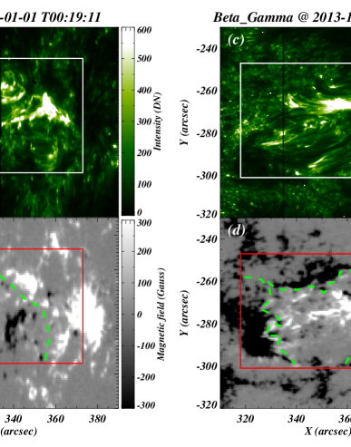
In Figure 1, we have displayed IRIS/SJI 1400 Å intensity maps of AR11937 (first type; (panel a)) and AR11934 (first - type; panel c). The first type AR11937 (first observation of the table 1) and the first - type AR 11934 (sixth observation of the table 1) were observed on January 1st, 2014 and December 27th, 2013, respectively. The overplotted white boxes in panels (a) and (c) outline the region of interest (ROI) in both types of AR and ROI is filled with several cool loops.
Further, we have also displayed the Heliosesmic and Magnetic Imager (HMI) line-of-sight (LOS) magnetogram of AR11937 (panel b) and AR11934 (panel d). In both LOS magnetograms, the black region corresponds to negative polarity while the white region corresponds to positive polarity. Here, please note that the red rectangular boxes on these magnetograms display the same ROI as shown by white boxes in panels a & c. In case of AR11937 (i.e., panel b), we have drawn the polarity inversion line (PIL) by green dashed line that clearly distinguish the positive and negative polarity, and one PIL is sufficient to separate positive and negative polarity. The existence of only one PIL justifies that AR11937 has a simple bipolar nature, and it is categorized as type AR. On the contrary, at least, we need three different PILs (see three green dashed lines within the red box in panel d) to draw the boundary between positive and negative polarity in the magnetogram of AR11934. Hence, unlike the AR11937, the presence of three different PILs justify that this AR11934 has a complex configuration of the magnetic field. Therefore, AR11934 is a - type AR. Later, we checked the LOS magnetograms of all ARs, and we found that five out of 10 observations are type ARs while the rest five observations are of – type AR (see table 1). All the necessary details of all and – type ARs are tabulated in the table1. Further, please note that the information about the types of ARs are mentioned on the solar monitor website111www.SolarMonitor.org, and our classification is consistent with the information provided on the solar monitor website.
| Sr. No. | Type of AR | AR Number | Date Time | Exposure/Cadence Time (s) | Central coordinates (x,y) | |
|---|---|---|---|---|---|---|
| 1 | Beta | AR11937 | 2014-01-01 00:04:31-00:39:13 | 3.99/5.2 | 343", -237" | 0.900 |
| 2 | Beta | AR12641 | 2017-03-02 12:31:35-14:21:43 | 3.99/5.2 | -179", 373" | 0.902 |
| 3 | Beta | AR12832 | 2021-06-11 13:09:55-13:58:52 | 7.99/9.2 | 295", 235" | 0.919 |
| 4 | Beta | AR12458 | 2015-11-26 01:37:27-02:27:27 | 7.99/9.4 | -559", 138" | 0.800 |
| 5 | Beta | AR12692 | 2017-12-23 00:40:21-01:29:27 | 7.99/9.2 | -290", 343" | 0.883 |
| 6 | Beta-Gamma | AR11934 | 2013-12-27 21:02:38-21:36:29 | 3.99/5.1 | 324",-270" | 0.898 |
| 7 | Beta-Gamma | AR12712 | 2018-06-01 00:05:42-01:32:07 | 14.99/16.2 | 299",279" | 0.904 |
| 8 | Beta-Gamma | AR13226 | 2023-02-15 13:11:59-14:38:23 | 14.99/16.2 | -234",281" | 0.924 |
| 9 | Beta-Gamma | AR10317 | 2022-05-24 05:36:48-06:25:45 | 7.99/9.2 | 521",235" | 0.803 |
| 10 | Beta-Gamma | AR13180 | 2023-01-04 08:41:24-09:30:30 | 7.99/9.2 | -223",380" | 0.888 |
We have utilized uncalibrated (i.e., data numbers (DN/s)) as well as calibrated spectra (i.e., erg/cm2/s/sr) in the present work. We have used irisgetwindata.pro routine with calib keyword to get calibrated spectra. It is to be noted that we have used the latest version (version - 009) of iris calibration to get the calibrated spectra. The same routine is used with the norm keyword (and without calib keyword) to get uncalibrated spectra. In the next step, Si iv 1402.77 Å line is fitted with the single Gaussian function to get the peak (or central) intensity, centroid, and Gaussian width (i.e., ) at each location of ROI. It is also to be noted that Gaussian fit is applied on both uncalibrated and calibrated spectral profiles. Then, using peak intensity and Gaussian width, we have calculated the total intensity (i.e., the area under the curve) at each location of ROI. Again, it is to be noted that the total intensity is estimated in DN/s as well as erg/cm2/s/sr. Further, the Gaussian width is converted into full width at half maximum (FWHM) using FWHM = 2.3548Gaussian width, and the centroid is converted into the Doppler velocity with the help of the rest wavelength of Si iv line. Here, it should be noted that estimating the rest wavelength is crucial as it can directly affect the Doppler velocity. There are three different methods to calculate the rest wavelength, namely, limb method, chromospheric method, and lamp method (Peter &
Judge 1999).
The present work utilizes the neutral/single ionized lines (i.e., cool lines) to estimate the rest wavelength of the Si iv line. Usually, the cool photospheric/chromospheric lines have low systematic Doppler shifts, and this low systematic Doppler shift is considered the least plasma flow that exists in the solar atmosphere. Therefore, cool photospheric/chromospheric lines are used in this method to calibrate the rest wavelength of any spectral line.
| Sr. No. | Type of AR | Cool spectral line | Centroid of cool spectral line (Å) | Difference (Observed Centroid - Standard Centroid)(Å) | Rest Wavelength for Si iv (Å) |
|---|---|---|---|---|---|
| 1 | Beta | Fe ii | 1405.6050 | -0.0030 | 1402.7730 |
| 2 | Beta | S i | 1401.5151 | 0.0016 | 1402.7716 |
| 3 | Beta | S i | 1401.5049 | -0.0086 | 1402.7786 |
| 4 | Beta | Fe ii | 1405.5991 | -0.0090 | 1402.7790 |
| 5 | Beta | S i | 1401.5116 | -0.0019 | 1402.7719 |
| 6 | Beta-Gamma | Fe ii | 1405.5064 | -0.0072 | 1402.7772 |
| 7 | Beta-Gamma | S i | 1401.5061 | -0.0074 | 1402.7774 |
| 8 | Beta-Gamma | Fe ii | 1405.6034 | -0.0066 | 1402.7766 |
| 9 | Beta-Gamma | Fe ii | 1405.6022 | -0.0078 | 1402.7778 |
| 10 | Beta-Gamma | S i | 1401.5079 | -0.0056 | 1402.7756 |
IRIS provides several cool lines that can be used in the rest wavelength estimation. And, we have utilized Fe ii and S i lines to calculate the rest wavelength. We have followed the same procedure as described in the IRIS Technical Note 20 available at IRIS/LMSAL website222https://iris.lmsal.com/search/. Finally, in table 2, we have tabulated all the necessary information related to the rest wavelength estimation, namely, used cool lines, observed centroid of cool lines, the difference between observed centroids and standard wavelength of cool lines (i.e., taken from CHIANTI database), and, the rest wavelength of Si iv. Using the estimated rest wavelength, the centroids are converted into the Doppler velocity.
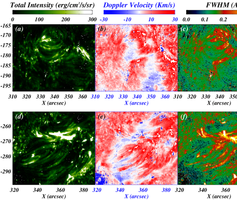
The integrated (total) calibrated intensity(panel a), Doppler velocity (panel b), and FWHM maps (panel c) of ROI from the first AR are displayed in the top row of figure 2. Similarly, the bottom row displays total calibrated intensity (panel d), Doppler velocity (panel e), and FWHM maps (panel f) of the first – AR.
3 Results
3.1 The Selection of the Foot Points of Cool loops
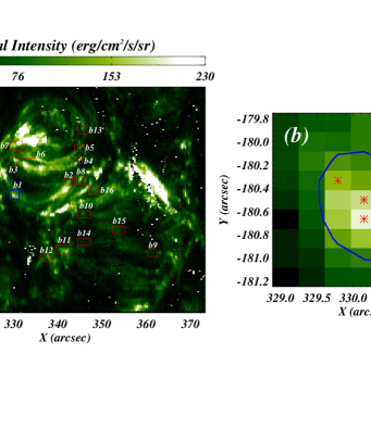
We have displayed integrated calibrated intensity maps (ROI) of the first type AR panel (a) and the first - type AR panel (c) of the figure 3. Several footpoints of cool loops are clearly visible in both ARs (see panels (a) and (c)). We have selected, manually, 16 different boxes (displayed by red boxes) in the vicinity of the foot points of the cool loops in the type AR (panel a) and 20 boxes in the - type AR (panel c). One particular box, which is shown in blue color in panel (a), is further shown in panel (b) of figure 3. Similarly, the blue color box of panel (c) is displayed in panel (d) of figure 3.
Major area of both boxes shown in panels (b) (d) has a bright region (i.e., foot point). However, a small fraction of the area of these boxes are less bright (i.e., non-footpoint region) and is most probably not related to the footpoints of the cool loops. To exclude this non-footpoint region in these boxes, we have calculated the mean intensity of that particular box (i.e., an average of the integrated calibrated intensities over all the pixels of that particular box. For instance, the average intensity of boxes shown in panels (b) and (d) are 94.82 and 751.34, respectively.) Further, using this mean intensity value as an intensity threshold, we draw the contour within each box, i.e., the blue contours in panels (b) and (d) of figure 3. Now, the region inside the blue contour is considered as the footpoint region while the region outside of the blue contour is the non-footpoint region. We have applied the above-described procedure to all boxes of all five and five – type ARs. Here, it is to be noted that we have provided the mean calibrated intensity of each box from all and – ARs in the appendix B.
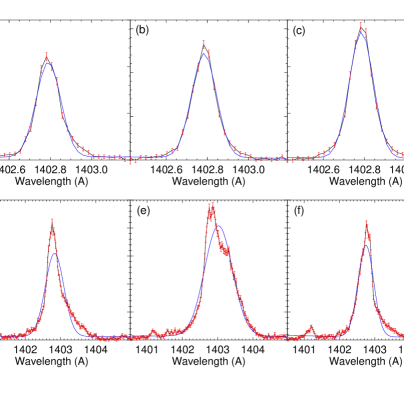
Then, we collected integrated calibrated intensity, integrated uncalibrated intensity Doppler velocity, and FWHM from each location of the footpoints, i.e., from only bright regions in each box of all five type ARs and – type ARs. To show the spectra from loop footpoints, we have chosen three locations in the vicinity of footpoints of AR (see asterisk signs in panel b; Figure 3) and three more locations in - AR (see, three asterisk signs in panel (d); Figure 3). The top row of Figure 4 shows the spectra (black solid curve) from the three locations of the panel (b) of Figure 3. Similarly, spectra from the three locations of footpoints of - AR are displayed in the bottom row of Figure 4. The blue curve in all panels of Figure 4 are the Gaussian fit on the corresponding observed profile. Here, it is clearly visible that spectral profiles in - AR are far more complex than the spectral profiles in AR.
3.2 Statistical Analysis of the Footpoints of Cool loops
First of all, we would like to mention that the ARs, which we have used in the present analysis, span the period of more than 9 years, i.e., from 2013 to 2023 (see table 1). We know that all the instruments, including IRIS, degrade with time. Hence, the instrumental degradation aspect should be included in this comparative analysis. Therefore, we have compared the calibrated as well as uncalibrated intensities of the loop footpoints (Figure 5) from two ARs that are close in time, i.e., first AR (i.e., AR11937) that was observed on 2014-01-01 and the first - AR (i.e., AR11934) that was observed on 2013-12-27. The time difference between AR11937 and AR11934 is just 4 days. Hence, the instrument degradation effect would have not been present (at least) between these two ARs.
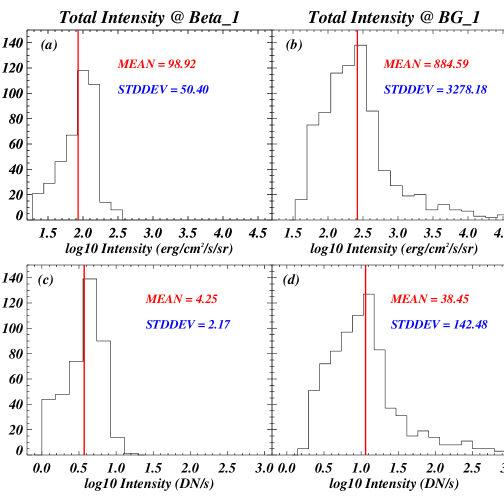
The mean of integrated calibrated (erg/cm2/s/sr) intensity of the loop footpoints is 99 and 885 in the first (panel a; Figure 5) and first – ARs (panel b; Figure 5), respectively. It means that the integrated calibrated intensity of the loop’s footpoints in the first – AR is nearly 9 times the corresponding integrated calibrated intensity in the AR. Similarly, the mean of uncalibrated intensity (i.e., DN/s) of loop footpoints in the first – AR (i.e., 38.45; panel d of Figure 5) is also nearly 9 times the corresponding mean of uncalibrated intensity of first AR (i.e., 4.25; panel c; Figure 5). Hence, we can say that the calibrated as well as uncalibrated intensities of the loop footpoints do show almost the same behavior.
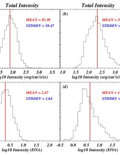
Further, in the next step, we have produced the histograms of the calibrated intensities and uncalibrated intensities of the loop footpoints from all five and - ARs (Figure 6). Now, the mean calibrated intensity of the loop footpoints in – type ARs (panel b) is more than 4 times the intensity of the loop footpoints in type ARs (panel a; Fig 6). The mean uncalibrated intensity of the loop footpoints in – ARs (panel d) is also more than 4 times the intensity of the loop footpoints in ARs (panel c; Fig 5). Hence, the same intensity difference is reduced to less than half (i.e., 4 times) if we consider all the ARs together (over different years), see Figure 6.
Most of the ARs (i.e., four out of five observations) were observed from January 2014 to December 2017. Most of the – ARs (four out of five) were observed from June 2018 to February 2023. Hence, the effect of instrumental degradation is more on the – ARs than ARs. Even after the dominant effect of instrumental degradation on – ARs, the mean intensity of – ARs is more than 4 times higher than the corresponding intensity of ARs. Although, the same difference is found to be around 9 times for both type ARs observed nearly at the same time (Figure 5). The reduction in the intensity difference (when we consider all the ARs together) is due to the instrumental degradation as the ARs cover a period of more than 9 years.
Perhaps, the footpoints of cool loops may be contaminated by the emission coming from the lower solar atmosphere, i.e., plage emission from the solar chromosphere. In the current observational baseline, it is hard to estimate the plage contribution into the loop footpoints. However, we have tried to understand the contribution by the plage into the loop footpoints. For this, we have analyzed chromospheric intensity of all boxes in the first and first – ARs (as shown in Figure 3) using IRIS/SJI 2796 Å. We have found that mean chromospheric intensity (i.e., averaged over all boxes) is nearly same in both types of ARs. Hence, if plage emission (i.e., chromospheric emission) contributes to the loop footpoints in TR then, this contribution is almost same in the footpoints of cool loops of and – ARs. Therefore, we are lead to believe that differences in the loop footpoint intensities are due to the TR activities, and not due to the plage contamination.
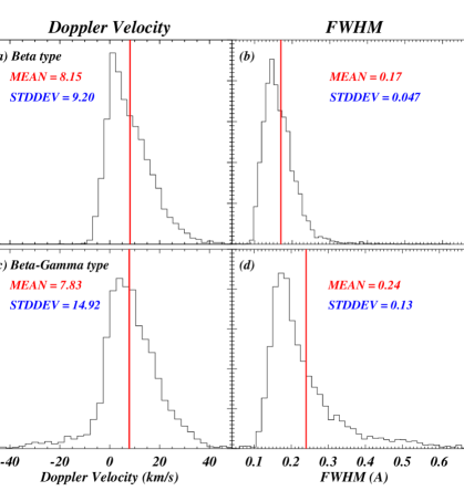
The histograms of the Doppler velocity and FWHM of all five and five – ARs are shown in figure 7. The mean Doppler velocity in ARs is 8.159.20 km/s (panel a) and in – ARs is 7.8314.92 km/s (panel c). Then, the mean FWHM of and – ARs are 0.170.047 Å (panel b) and 0.240.13 Å (panel d), respectively. The solid red vertical line in each panel of figure 7 shows the mean values of the corresponding parameters. Further, we have mentioned mean and standard deviation values in each panel. The mean FWHM of the loop footpoints in - ARs is significantly higher (i.e., almost 1.5 times) than the mean FWHM of ARs. Here, it should also be noted that the spread of the FWHM histograms of – ARs is around 3 times higher than the corresponding spread of FWHMs in ARs. This higher FWHM and more spread justify the higher activity level at the footpoints of cool loops in - ARs. On the contrary the mean Doppler velocity of both and – ARs are almost the same. But the spread of the Doppler velocity in - ARs is more than 1.5 times higher than the corresponding spread of Doppler velocity in ARs. On the contrary, the mean Doppler velocities for both types of ARs are almost the same (see panels a and c of Figure 7). Here, it should be noted that the spread of Doppler velocity distribution in - ARs is more than 1.5 times the corresponding spread of Doppler velocity in ARs.
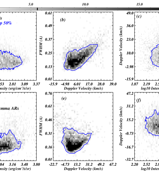
The 2D histograms of peak calibrated intensity–FWHM (panel a), Doppler Velocity–FWHM (panel b), and peak calibrated intensity–Doppler Velocity (panel c) for the footpoints of the loops of type ARs are displayed in the figure 8. The same correlations for the loop footpoints in – ARs are displayed in the panels (d), (e), and (f) of figure 8. The white color corresponds to the lowest histogram density (i.e., zero density) while the black color shows the highest histogram density in all 2D histograms. The colorbar at the top of this figure 8 represents the variations of histogram density. We sorted the non-zero densities of each histogram, and then we estimated the histogram density value at the middle location. For example, 2D histograms of peak calibrated intensity–FWHM (panel a) have a total of 1286 non-zero histogram density points. Now, we sorted 1286 histogram density points in increasing order, and we found that the histogram density value at the middle location (i.e., at location number 643) is 5. Then, we used this value (i.e., 5) as a threshold value to draw contour on the 2D histograms of peak calibrated intensity–FWHM (see blue contour; panel a). The same procedure is applied to other 2D histograms to draw the blue contours. Finally, we mention that blue contours in each 2D histogram enclose the highest 50 % histogram densities.
In the case of ARs, the peak calibrated intensities and FWHM are not correlated (panel a). However, in the case of - ARs, peak calibrated intensity are weakly (positively) correlated with FWHM (panel d). The Doppler velocity is well (positively) correlated with FWHM in both types of ARs (see panels (b) and (e)). While, on the contrary, we do not see any profound correlation between peak calibrated intensity and Doppler velocity of the footpoints of the cool loops in the type ARs (panel c) and - type ARs (panel f).
3.3 Line Ratios of Si iv (1394/1403) in the Footpoints of loops
The intensity ratio of Si iv resonance lines (i.e., 1393.75/1403.77) is an important measure of the opacity. Generally, it is assumed that Si iv lines form in optically thin conditions. However, this is not the case always, and Si iv spectral lines may also form in the optically thick conditions (e.g., Yan et al. 2015; Tripathi et al. 2020; Kayshap et al. 2021). Theoretically, we know that the intensity of Si iv 1393.755 Å is double the intensity of Si iv 1402.77 Å (e.g., Dere et al. 1997; Dere
et al. 2019). Hence, the intensity ratio must be 2 if the lines are forming in optically thin conditions. Hence, simply, with the help of this intensity ratio, we can understand whether the line is forming under optically thin or thick conditions. (Tripathi et al. 2020; Kayshap et al. 2021).
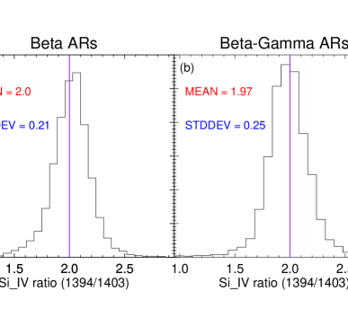
The figure 9 shows the histograms of intensity ratio for the loop footpoints in ARs (left panel) as well as – ARs (right panel). In both histograms, the vertical solid purple line shows the location of the theoretical intensity ratio (i.e., 2.0). The ratio values are almost ranging from 1.3 to 2.6 in both AR types. The mean ratio values are 2.0 and 1.97 for and – ARs. Hence, the mean ratio is found to be slightly low for the footpoints in - type ARs than that for type ARs. The spread of ratio values (i.e., standard deviation) is more in - type ARs (0.25) than type ARs (i.e., 0.21).
Further, we have searched the locations where the ratio significantly deviates from the theoretical ratio (i.e., 2). To know this, first of all, we have chosen the locations where the line ratios are less than 1.90 and the line ratios are greater than 2.10. In the case of the footpoints of ARs, there are 23% locations which are having a ratio of less than 1.90, and almost 29% locations which are having a ratio greater than 2.10. Similarly, in the case of the footpoints of - ARs, 31% locations are having a ratio less than 1.90, and almost 24% locations are having ratios greater than 2.10. In total, around 52% locations in ARs and 55% locations in - ARs are significantly deviated from the theoretical ratio. Hence, it is factually established that Si iv spectral lines originating from more than half of the locations of the footpoints of cool loops are formed in optically thick conditions.
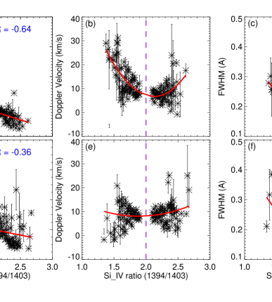
We have created 500 bins from the significant line ratios (i.e., only the line ratios less than 1.90 and greater than 2.10). Further, we have collected the corresponding parameters (i.e., intensity, Doppler velocity, and FWHM) in each ratio bin, and then calculated the mean and standard error of each parameter in each ratio bin. Hence, through this approach, we have obtained 500 mean values and standard errors for each parameter. Then, using these mean values and standard errors, we have performed some correlations shown in figure 10, namely, (1) line ratio vs. total calibrated intensity for ARs (panel a) and - ARs (panel d), (2) line ratio vs. Doppler velocity for ARs (panel b) and - ARs (panel e), and (3) line ratio vs. FWHM for ARs (panel c) and - ARs (panel f). In both and – ARs, the total calibrated intensity is high when the Si iv ratio is less than 1.90. If the Si iv ratio is greater than 2.10 then the total calibrated intensity is low (see panels (a) and (d)). On the contrary, for and – ARs, the redshifts (Doppler velocity) increase in both cases whether the line ratio goes down below 1.90 or it increases beyond 2.10 (see panels b and e). The same behavior is found for FWHM in both types of ARs, see panels (c) and (f). Here, it is to be noted that the above-described pattern of Doppler velocity with line ratio is weak in – ARs (panel e) in comparison to the same correlation for ARs (panel b). However, the correlation of FWHM with line ratio is strong in both types of ARs (see panels c and f).
3.4 Complexity of Spectral Profiles
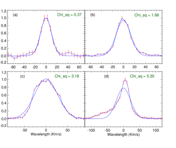
Finally, during the analysis, we noticed that not all the spectral profiles are single Gaussian, but some spectral profiles deviate from the single Gaussian. We have estimated the chi-square value for each location in the footpoints of cool loops, and we produced the histogram of (left-panel; Figure 7) as well as - type ARs (right-panel; Figure 11).
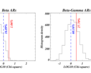
The blue dashed vertical line is located at the reduced chi-square value of 1 in both panels. Interestingly, there are more than 16% complex profiles (i.e., profiles having reduced chi-square values greater than 1) in the loop footpoints of ARs. While - ARs have more than 60% complex profiles. Hence, we can say that the footpoints of the loops in - type ARs have 3.7 times more complex profiles than that in type ARs.
In general, if the chi-square value is greater than one, the profile is said to be asymmetric. However, we can consider the profile as a single Gaussian up to a specific chi-square value, for example, Rao
et al. 2022 shows that a spectral profile with a chi-square value less than 5 can be effectively fitted with a single Gaussian. However, they drew their conclusion based on QS observations. While we are dealing with ARs, and, therefore, the chi-square threshold value may differ.
We have investigated the spectral profiles with respect to the chi-square value (see appendix A), and it is found that the spectral profiles having chi-square values less than 3 can be well fitted with a single Gaussian (appendix A)). Therefore, in the present work, we used 3 as a chi-square threshold value to define the complex profiles. The solid red lines, in both panels, are at the threshold value of the chi-square (i.e., 3). Interestingly, the very complex profiles in the loop footpoints of – ARs are more than 26 times the complex profiles in type ARs. This observational finding justifies that the footpoints of cool loops have high complex behaviour in - type ARs than the simple type ARs.
4 Summary and Discussion
The present work is to statistically investigate the footpoints of cool loops using IRIS and HMI/SDO observations. IRIS has revealed that cool loops are an integral part of ARs (e.g., Huang et al. 2015; Rao et al. 2019a, b). In the present work, we have taken five type ARs and five – type ARs to diagnose the footpoint of cool loops. Further, a comparison is also performed between the properties of the footpoints of these cool loops in and – type ARs. Through the statistical approach, we have derived some important findings about the footpoints of cool loops, which are summarized below.
-
•
The mean calibrated and uncalibrated intensities from first AR are 98.9250.40 erg/cm2/s/sr and 4.252.17 DN/s, respectively. The same intensities for first – AR are 884.593278.18 erg/cm2/s/sr and 38.45142.48 DN/s.
-
•
Similarly, the mean calibrated and uncalibrated intensities from all five ARs are 92.3858.47 erg/cm2/s/sr and 2.471.64 DN/s, respectively. The same intensities are 396.651533.52 erg/cm2/s/sr and 11.4966.37 DN/s but for all five – ARs.
-
•
The mean Doppler velocity and FWHM of the footpoints of the cool loops in all five type ARs are 8.159.20 km/s, and 0.170.047 Å, respectively. The same parameters are 7.8314.92 km/s and 0.240.13 Å but for all five – ARs.
-
•
The mean calibrated and uncalibrated intensities are 9 times stronger in the – AR in comparison to the AR if we consider both AR close in time, i.e., no instrumental degradation. The same intensity difference is reduced to 4 times if we consider all the ARs. These ARs are observed over 9 years, therefore, the reduction in the intensity difference is most probably due to the instrumental degradation.
-
•
There is no correlation between the central (peak) calibrated intensity and FWHM, and between the central calibrated intensity and Doppler velocity of the footpoints of the loops in as well as - type ARs. However, the Doppler velocity and FWHM of the cool loop footpoints in both types of ARs are weakly correlated.
-
•
The Si iv line ratios from the footpoints of cool loops in both types of ARs are significantly deviated from the theoretical intensity ratio of Si iv. Here, we find that the opacity is important for more than half of the footpoint locations.
-
•
If the line ratio drops below 1.90 then the intensity of the footpoints becomes stronger. The intensity is getting weaker when the ratio goes beyond 2.10. However, the Doppler velocity and FWHM increase for low (i.e., the ratio less than 1.90) as well as high ratio values (i.e. ratio greater than 2.10).
-
•
Lastly, we find that the footpoints of cool loops have more complex profiles in - type ARs (i.e., 27.70%) than that in type ARs (i.e., 1.06%). The complex profiles are almost 26 times higher in - type ARs than that in the type ARs.
This is the first-ever research that demonstrates the complexity of ARs affecting, directly, the mean attributes of the footpoints of the cool loops. We examined a total of 200 footpoints of the cool loops from both types of ARs, i.e., 120 footpoints in type ARs and 80 footpoints in – type ARs. Statistically, we have found significantly higher mean intensities of the loop footpoints in the complex – type ARs than that in type ARs. We know that any instrument including IRIS degrades with time. Hence, the intensities from – are significantly affected due to the instrumental degradation because most of – ARs are observed later than ARs. Hence, the intensity differences between the loop footpoints of – ARs and ARs (, i.e., loop footpoints in – ARs have 4 times higher intensity than the corresponding intensity in ARs) are underestimated.
The plasma flows within the footpoints of cool loops are almost similar in both types of AR. In this analysis, we have considered blueshifted and redshifted footpoints of cool loops, and it is found that the majority of the footpoints are redshifted. The mean redshifts of these footpoints are around 8.0 km/s in both types of AR. In general, solar TR of quiet-Sun, coronal hole, and ARs are red-shifted (Teriaca
et al. 1999; Peter 1999; Peter &
Judge 1999; Dadashi
et al. 2011; Kayshap et al. 2015; Kayshap &
Dwivedi 2017). In the present analysis, similar to previous works, we have also found that the footpoints of the cool loop in both ARs are redshifted. Please note that the Doppler velocity of ARs varies as per the location of the AR on the solar disk, i.e., center-to-limb variations (CLV) do exist in the Doppler velocity of ARs (e.g., Ghosh
et al. 2019; Rajhans et al. 2023). The Doppler velocity is maximum at the disk center which decreases while moving toward the solar limb. The Doppler velocity near the disk center is around 7–9 km/s (Rajhans et al. 2023). In the present work, most of the ARs are close to the disk center (see the values in table 1), and the on-average Doppler velocity of footpoints of cool loops is 8.0 km/s. It (i.e., the mean value of Doppler velocity) is consistent with previously reported Doppler velocity of the footpoints of cool loops (e.g., Rao et al. 2019b, a) and ARs (Rajhans et al. 2023).
The footpoints of the cool loops exhibit large variations in the FWHM as shown by Rao et al. (2019b), i.e., 0.095–0.246 (first set of observations), 0.094–0.200 (second set of observations), and 0.125–0.182 (third set of observations). Earlier, Huang
et al. (2015) also showed broad spectral profiles at the footpoints of cool loops. Recently, Srivastava
et al. (2020) have found large FWHM (more than 0.25 Å) around the footpoint of the cool loops. The present work systematically estimates the FWHM in the footpoints of cool loops in both types of ARs. The spreads of FWHM are 0.10–0.40 Å and 0.10–0.70 Å in the footpoints of the cool loops in and ARs, respectively, and the reported range is consistent with the previous findings (e.g., Rao et al. 2019a, b). Most importantly, the mean FWHM in the loop footpoints is higher in – ARs than ARs. In addition, the spread in FWHM is more than 2 times in the footpoint of the cool loops in - than type ARs. In conclusion, both aspects justify higher activity levels in the loop footpoints of – ARs than ARs.
The line with high oscillator strength is affected the most due to opacity, and therefore, we do observe the reduced ratio, i.e., less than 2.0. The magnetic reconnection triggers various dynamic events within the lower solar atmosphere, like explosive events, and small-scale brightening (e.g., Isobe
et al. 2007; Peter
et al. 2014; Gupta &
Tripathi 2015; Kayshap &
Dwivedi 2017). Such events can enhance the electron density along the line of sight (LOS), and as a result, a thick atmosphere will form. The reabsorption probability of Si iv 1393.78Å photon in the thick atmosphere is twice in comparison to that of Si iv 1402.77 Å. Hence, the intensity of Si iv 1393.78Å reduces more and more as electron density increases in the LOS, and as a result, the ratio reduces more and more. In the present study, 23% locations in ARs and 31% locations in – ARs have ratio values less than 1.90 (i.e., significantly less than 2), and we know that footpoints of the cool loops are much prone area to the dynamic events mentioned above (e.g., Huang
et al. 2015; Huang et al. 2019; Rao et al. 2019a, b; Srivastava
et al. 2020). In addition, we have seen complex spectral profiles in the footpoints of the cool loop which are most probably due to the occurrence of magnetic reconnection in the vicinity of footpoints. Hence, such events at the loop footpoints have enhanced the opacity, and it is reflected as the reduced ratio of Si iv lines. On the other hand, 29% locations in ARs and 24% locations in – ARs have an intensity ratio greater than 2.10, and the intensity ratio higher than 2 is due to the resonant scattering (e.g., Wood &
Raymond (2000); Gontikakis &
Vial (2018); Tripathi et al. (2020)). Hence, it may also be possible that the resonant scattering is happening in the vicinity of footpoints. While further studies based on the modelling of Si iv lines are required to know this issue in great detail.
The estimation of the chi-square value is necessary to know the level of complexity in the spectral profiles. The chi-square analysis establishes that - type ARs have more than 26 times more complex profiles than the complex profiles of type ARs. Hence, we can say that the footpoints of cool loops are much more complex in - type ARs than that in type ARs. In addition, we have also noticed complex profiles (i.e., non-Gaussian, broad, and multi-peak profiles) within the footpoints of cool loops of both ARs and similar observational findings are already reported (e.g., Huang
et al. 2015; Rao et al. 2019b; Srivastava
et al. 2020).
In conclusion, we find that the footpoints of the cool loop in ARs are far more complex than that in type ARs, and the intensity FWHM are higher in – ARs than those in type ARs. On the contrary, the Doppler velocities are the same in both ARs.
Acknowledgements
We gratefully acknowledge the reviewer (Dr. Jaroslav Dudík) for his constructive comments that substantially improved the manuscript. B. Suresh Babu and P. Kayshap express gratitude and acknowledgment to Dr. Georgios Chintzoglou (LMSAL)and Dr. Bart De Pontieu (LMSAL) for the valuable inputs during a discussion at Hinode-16/IRIS-13 meeting. Based on their suggestions, we modified the analysis, particularly for the Si iv ratio estimation. P. Jelínek acknowledges support from grant 21-16508J of the Grant Agency of the Czech Republic. IRIS is a NASA small explorer mission developed and operated by LMSAL with mission operations executed at NASA Ames Research Center and major contributions to downlink communications funded by ESA and the Norwegian Space Centre. We also acknowledge the use of HMI/SDO.
Data Availability
The data underlying this article are available at https://iris.lmsal.com/data.html (NASA/IRISwebsite) and at https://iris.lmsal.com/search/(LMSAL search website). Note that IRIS data are publicly available with the observation ID OBS 3630088076, OBS 3620106076, OBS 3620108077, OBS 3840257196, OBS 3610108077, OBS 3860257446, OBS 3620110077, OBS 3620110077, OBS 3620108077, OBS 3610108077.
References
- Bethge et al. (2012) Bethge C., Beck C., Peter H., Lagg A., 2012, A&A, 537, A130
- Brekke et al. (1997) Brekke P., Hassler D. M., Wilhelm K., 1997, Sol. Phys., 175, 349
- Chae et al. (2000) Chae J., Wang H., Qiu J., Goode P. R., Wilhelm K., 2000, ApJ, 533, 535
- Dadashi et al. (2011) Dadashi N., Teriaca L., Solanki S. K., 2011, A&A, 534, A90
- Dadashi et al. (2012) Dadashi N., Teriaca L., Tripathi D., Solanki S. K., Wiegelmann T., 2012, A&A, 548, A115
- De Pontieu et al. (2014) De Pontieu B., et al., 2014, Sol. Phys., 289, 2733
- Del Zanna (2008) Del Zanna G., 2008, A&A, 481, L49
- Del Zanna, G. & Mason, H. E. (2003) Del Zanna, G. Mason, H. E. 2003, A&A, 406, 1089
- Del Zanna et al. (2011) Del Zanna G., O’Dwyer B., Mason H. E., 2011, A&A, 535, A46
- Dere et al. (1997) Dere K. P., Landi E., Mason H. E., Monsignori Fossi B. C., Young P. R., 1997, A&AS, 125, 149
- Dere et al. (2019) Dere K. P., Zanna G. D., Young P. R., Landi E., Sutherland R. S., 2019, The Astrophysical Journal Supplement Series, 241, 22
- Domingo et al. (1995) Domingo V., Fleck B., Poland A. I., 1995, Sol. Phys., 162, 1
- Doyle et al. (2006) Doyle J. G., Taroyan Y., Ishak B., Madjarska M. S., Bradshaw S. J., 2006, A&A, 452, 1075
- Dudík et al. (2017) Dudík J., Polito V., Dzifčáková E., Del Zanna G., Testa P., 2017, ApJ, 842, 19
- Ghosh et al. (2019) Ghosh A., Klimchuk J. A., Tripathi D., 2019, ApJ, 886, 46
- Gontikakis & Vial (2018) Gontikakis C., Vial J. C., 2018, A&A, 619, A64
- Gupta & Nayak (2022) Gupta G. R., Nayak S. S., 2022, MNRAS, 512, 3149
- Gupta & Tripathi (2015) Gupta G. R., Tripathi D., 2015, ApJ, 809, 82
- Hale et al. (1919) Hale G. E., Ellerman F., Nicholson S. B., Joy A. H., 1919, ApJ, 49, 153
- Hansteen et al. (2014) Hansteen V., et al., 2014, Science, 346, 1255757
- Harrison et al. (1995) Harrison R. A., et al., 1995, Sol. Phys., 162, 233
- Huang et al. (2015) Huang Z., Xia L., Li B., Madjarska M. S., 2015, The Astrophysical Journal, 810, 46
- Huang et al. (2019) Huang Z., Li B., Xia L., Shi M., Fu H., Hou Z., 2019, ApJ, 887, 221
- Isobe et al. (2007) Isobe H., Tripathi D., Archontis V., 2007, ApJ, 657, L53
- Kayshap & Dwivedi (2017) Kayshap P., Dwivedi B. N., 2017, Sol. Phys., 292, 108
- Kayshap et al. (2015) Kayshap P., Banerjee D., Srivastava A. K., 2015, Sol. Phys., 290, 2889
- Kayshap et al. (2021) Kayshap P., Singh Payal R., Tripathi S. C., Padhy H., 2021, MNRAS, 505, 5311
- Peter (1999) Peter H., 1999, ApJ, 522, L77
- Peter (2000) Peter H., 2000, A&A, 360, 761
- Peter (2001) Peter H., 2001, A&A, 374, 1108
- Peter (2006) Peter H., 2006, A&A, 449, 759
- Peter (2010) Peter H., 2010, A&A, 521, A51
- Peter & Judge (1999) Peter H., Judge P. G., 1999, ApJ, 522, 1148
- Peter et al. (2014) Peter H., et al., 2014, Science, 346, 1255726
- Polito et al. (2016) Polito V., Del Zanna G., Dudík J., Mason H. E., Giunta A., Reeves K. K., 2016, A&A, 594, A64
- Rajhans et al. (2023) Rajhans A., Tripathi D., Kashyap V. L., Klimchuk J. A., Ghosh A., 2023, ApJ, 944, 158
- Rao et al. (2019a) Rao Y. K., Srivastava A. K., Kayshap P., Dwivedi B. N., 2019a, Annales Geophysicae, 37, 765
- Rao et al. (2019b) Rao Y. K., Srivastava A. K., Kayshap P., Wilhelm K., Dwivedi B. N., 2019b, ApJ, 874, 56
- Rao et al. (2022) Rao Y. K., Del Zanna G., Mason H. E., 2022, Monthly Notices of the Royal Astronomical Society, 511, 1383
- Reale (2010) Reale F., 2010, Living Reviews in Solar Physics, 7
- Srivastava et al. (2020) Srivastava A. K., et al., 2020, ApJ, 894, 155
- Teriaca et al. (1999) Teriaca L., Banerjee D., Doyle J. G., 1999, A&A, 349, 636
- Tripathi et al. (2012) Tripathi D., Mason H. E., Zanna G. D., Bradshaw S., 2012, The Astrophysical Journal Letters, 754, L4
- Tripathi et al. (2020) Tripathi D., Nived V. N., Isobe H., Doyle G. G., 2020, ApJ, 894, 128
- Ugarte-Urra et al. (2009) Ugarte-Urra I., Warren H. P., Brooks D. H., 2009, The Astrophysical Journal, 695, 642
- Warren & Brooks (2009) Warren H. P., Brooks D. H., 2009, ApJ, 700, 762
- Wilhelm et al. (1995) Wilhelm K., et al., 1995, Sol. Phys., 162, 189
- Winebarger et al. (2013) Winebarger A., Tripathi D., Mason H. E., Del Zanna G., 2013, ApJ, 767, 107
- Wood & Raymond (2000) Wood K., Raymond J., 2000, ApJ, 540, 563
- Yan et al. (2015) Yan L., et al., 2015, ApJ, 811, 48
- Young et al. (2012) Young P. R., O’Dwyer B., Mason H. E., 2012, ApJ, 744, 14
Appendix A Nature of Spectral Profiles
In this appendix, we have displayed some spectral profiles from the footpoints of cool loops of AR11937 (see panels (a) to (d); Figure 9) and - type AR 11934 (see panels (e) to (h); Figure 9).
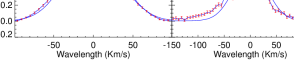
In each panel, the black solid line displays the observed spectra with corresponding errors in red color. The overplotted blue color line is the single Gaussian fit on the observed spectra. The reduced chi-square values are mentioned in each panel.
The observed spectra are well fitted by single Gaussian when the reduced chi-square values are less than 1 (see panels (a) (b) – profiles from AR, and panels (e) from AR). Although, the single Gaussian fits deviate as the chi-square value exceeds 3 (see panels (c) and (g)). Lastly, we mention that if the reduced chi-square value is much higher than 3 then single Gaussian, significantly, deviates from the observed spectra. Manually, we have checked several profiles from both types of AR, and it is found that the spectral profiles have chi-square values less than 3 can be characterized by a single Gaussian. Therefore, we have considered chi-square 3 as the threshold value.
Appendix B Mean Calibrated Intensities of all Boxes at loop Footpoint
In this appendix, we have shown the mean calibrated intensities of all selected boxes in all five and – ARs, namely, table 3 for the first (i.e., AR11937) and first – AR (i.e., AR11934), table 4 for second (i.e., AR12641) and second – AR (i.e., AR12712), table 5 for third (i.e., AR12832) and third – AR (i.e., AR13226), table 6 for fourth (i.e., AR12458) and fourth – AR (i.e., AR10317), and table 7 for fifth (i.e., AR12692) and fifth – AR (i.e., AR13180).
| Box. No. | Mean Intensity |
|---|---|
| b1 | 94.82 |
| b2 | 86.48 |
| b3 | 86.08 |
| b4 | 80.39 |
| b5 | 51.19 |
| b6 | 102.74 |
| b7 | 125.97 |
| b8 | 75.17 |
| b9 | 24.66 |
| b10 | 40.29 |
| b11 | 69.11 |
| b12 | 70.65 |
| b13 | 46.00 |
| b14 | 23.31 |
| b15 | 36.87 |
| b16 | 75.92 |
| Box. No. | Mean Intensity |
|---|---|
| b1 | 751.34 |
| b2 | 1650.98 |
| b3 | 150.11 |
| b4 | 246.08 |
| b5 | 282.70 |
| b6 | 177.18 |
| b7 | 204.71 |
| b8 | 552.47 |
| b9 | 244.19 |
| b10 | 130.35 |
| b11 | 92.00 |
| b12 | 103.23 |
| b13 | 58.40 |
| b14 | 630.00 |
| b15 | 39.63 |
| b16 | 61.10 |
| b17 | 19.60 |
| b18 | 130.23 |
| b19 | 47.75 |
| b20 | 51.85 |
| Box. No. | Mean Intensity |
|---|---|
| b1 | 90.18 |
| b2 | 58.29 |
| b3 | 112.49 |
| b4 | 85.82 |
| b5 | 93.01 |
| b6 | 90.64 |
| b7 | 139.50 |
| b8 | 100.29 |
| b9 | 53.81 |
| b10 | 51.68 |
| b11 | 49.48 |
| b12 | 65.52 |
| b13 | 68.20 |
| b14 | 32.77 |
| b15 | 31.19 |
| b16 | 35.89 |
| Box. No. | Mean Intensity |
|---|---|
| b1 | 144.37 |
| b2 | 97.69 |
| b3 | 54.65 |
| b4 | 53.03 |
| b5 | 190.97 |
| b6 | 128.44 |
| b7 | 98.93 |
| b8 | 81.64 |
| b9 | 46.18 |
| b10 | 37.66 |
| b11 | 86.30 |
| b12 | 65.27 |
| Box. No. | Mean Intensity |
|---|---|
| b1 | 43.93 |
| b2 | 57.44 |
| b3 | 31.64 |
| b4 | 76.18 |
| b5 | 72.22 |
| b6 | 33.27 |
| b7 | 51.25 |
| b8 | 36.83 |
| b9 | 37.30 |
| b10 | 40.41 |
| b11 | 24.20 |
| b12 | 22.67 |
| b13 | 66.67 |
| Box. No. | Mean Intensity |
|---|---|
| b1 | 302.71 |
| b2 | 154.46 |
| b3 | 771.70 |
| b4 | 227.58 |
| b5 | 131.70 |
| b6 | 417.15 |
| b7 | 106.17 |
| b8 | 151.48 |
| b9 | 968.28 |
| b10 | 148.63 |
| b11 | 128.41 |
| b12 | 59.28 |
| b13 | 139.02 |
| b14 | 156.00 |
| b15 | 94.91 |
| b16 | 66.96 |
| b17 | 80.42 |
| b18 | 73.92 |
| b19 | 127.94 |
| b20 | 64.22 |
| b21 | 141.44 |
| b22 | 160.10 |
| b23 | 114.51 |
| Box. No. | Mean Intensity |
|---|---|
| b1 | 25.11 |
| b2 | 23.81 |
| b3 | 37.84 |
| b4 | 53.62 |
| b5 | 65.02 |
| b6 | 54.71 |
| b7 | 19.59 |
| b8 | 39.95 |
| b9 | 33.21 |
| b10 | 39.52 |
| b11 | 35.04 |
| b12 | 47.43 |
| b13 | 14.07 |
| b14 | 21.38 |
| b15 | 24.10 |
| b16 | 46.52 |
| b17 | 41.84 |
| b18 | 29.54 |
| b19 | 20.36 |
| b20 | 19.99 |
| b21 | 65.40 |
| b22 | 27.38 |
| b23 | 20.42 |
| b24 | 22.97 |
| b25 | 12.30 |
| Box. No. | Mean Intensity |
|---|---|
| b1 | 152.28 |
| b2 | 271.07 |
| b3 | 93.75 |
| b4 | 168.74 |
| b5 | 282.74 |
| b6 | 153.67 |
| b7 | 197.77 |
| b8 | 100.07 |
| b9 | 140.35 |
| b10 | 149.20 |
| b11 | 110.04 |
| b12 | 142.64 |
| Box. No. | Mean Intensity |
|---|---|
| b1 | 87.12 |
| b2 | 66.12 |
| b3 | 123.33 |
| b4 | 89.60 |
| b5 | 135.68 |
| b6 | 76.61 |
| b7 | 118.24 |
| b8 | 67.19 |
| b9 | 90.48 |
| b10 | 57.24 |
| b11 | 72.43 |
| b12 | 52.39 |
| b13 | 124.57 |
| b14 | 87.52 |
| b15 | 74.63 |
| b16 | 43.38 |
| b17 | 58.50 |
| b18 | 53.38 |
| b19 | 70.0 |
| b20 | 52.14 |
| b21 | 109.29 |
| b22 | 34.76 |
| b23 | 91.69 |
| b24 | 42.82 |
| b25 | 48.14 |
| Box. No. | Mean Intensity |
|---|---|
| b26 | 47.87 |
| b27 | 83.46 |
| b28 | 47.41 |
| b29 | 95.81 |
| b30 | 126.27 |
| b31 | 67.35 |
| b32 | 123.55 |
| b33 | 128.52 |
| b34 | 194.62 |
| b35 | 46.15 |
| b36 | 80.54 |
| b37 | 29.00 |
| b38 | 54.17 |
| b39 | 60.03 |
| b40 | 77.69 |
| b41 | 79.53 |
| b42 | 96.69 |
| b43 | 92.05 |
| b44 | 117.48 |
| b45 | 104.87 |
| b46 | 70.97 |
| b47 | 66.22 |
| b48 | 78.14 |
| b49 | 65.55 |
| b50 | 59.51 |
| Box. No. | Mean Intensity |
|---|---|
| b1 | 125.44 |
| b2 | 187.04 |
| b3 | 124.65 |
| b4 | 170.00 |
| b5 | 122.18 |
| b6 | 98.70 |
| b7 | 81.47 |
| b8 | 51.07 |
| b9 | 125.14 |
| b10 | 58.44 |
| b11 | 71.00 |
| b12 | 33.51 |
| b13 | 29.88 |